1. Introduction
Closure of the meridional overturning circulation (MOC) of the oceans requires the upwelling of abyssal waters to the surface. In the Atlantic Ocean the MOC consists of two primary cells, a shallower cell forced by North Atlantic Deep Water (NADW) production in the Greenland, Iceland, Norwegian and Labrador Seas and an underlying deeper cell forced by Antarctic Bottom Water (AABW) production in the southern ocean surrounding the continent of Antarctica. It has recently been convincingly argued (Marshall & Speer Reference Marshall and Speer2012) that the upwelling of NADW in the Southern Ocean is accommodated primarily by wind-driven adiabatic processes in which horizontal advection is balanced by vertical advection rather than diapycnal diffusivity. However, the upward transfer of AABW to mid-depth in all ocean basins is strongly dependent upon the diabatic process of upward mixing of the weakly stratified abyssal waters (Lumpkin & Speer Reference Lumpkin and Speer2007; Talley Reference Talley2013). The importance of an effective turbulent diapycnal diffusivity through which such a cross-isopycnal flux of mass may be accommodated follows from the analysis of Munk (Reference Munk1966) and Munk & Wunsch (Reference Munk and Wunsch1998). The magnitude of the associated buoyancy flux that enables the upwelling of abyssal waters depends upon the irreversible component of the mixing that the turbulence is able to support, which depends upon its efficiency. The candidate mechanisms through which the required turbulent mixing is produced are numerous, and include convective, shear and double-diffusive processes, although the primary energy source is widely believed to be associated with the dissipation of the internal tide raised in the oceans by the flow of the astronomically forced barotropic tide over bottom topography (Garrett & Kunze Reference Garrett and Kunze2007; Salehipour, Stuhne & Peltier Reference Salehipour, Stuhne and Peltier2013). Because the ocean interior is stably stratified in density, this mechanism leads to the generation of a field of internal inertia gravity waves, the internal tide, which may ‘break’ and thereby dissipate through the above-stated mechanisms.
Of the available candidate mechanisms for generation of the required turbulence, one that is known to be involved in the abyssal ocean and to act in conjunction with the internal tide is that in which turbulence production is driven by the vertical shear of horizontal velocity when it is sufficiently strong to overcome the stabilizing influence of the density stratification (see e.g. van Haren et al.
Reference van Haren, Gostiaux, Morozov and Tarakanov2014). This is the classical mechanism of Kelvin (Reference Kelvin1871) and Helmholtz (Reference Helmholtz1868), which acts under circumstances in which a criterion based upon gradient Richardson number is exceeded, a criterion most elegantly captured in the Miles–Howard inviscid theorem (Howard Reference Howard1961; Miles Reference Miles1961). This theorem requires as a necessary but not sufficient condition for instability that an inviscid two-dimensional parallel shear flow that is stably stratified be one in which the number
 $\mathit{Ri}(z)=N^{2}/(\text{d}U/\text{d}z)^{2}$
is less than
 $1/4$
somewhere in the flow (here
 $N$
is the characteristic Brunt–Väisälä frequency of the stratification and
 $U$
is the horizontal velocity of the background flow).
Evidence of the action of the classical Kelvin–Helmholtz (KH) mechanism is abundant in geophysical observations on a wide range of scales in both the atmosphere (see e.g. Browning Reference Browning1971) and oceanic environments including gravity currents (Legg et al. Reference Legg, Ezer, Jackson, Briegleb, Danabasoglu, Large, Wu, Chang, Özgökmen, Peters, Xu, Chassignet, Gordon, Griffies, Hallberg, Price, Riemenschneider and Yang2009), equatorial undercurrents (Moum, Nash & Smyth Reference Moum, Nash and Smyth2011), estuarine shear zones (Geyer et al. Reference Geyer, Lavery, Scully and Trowbridge2010) and the abyssal ocean (van Haren et al. Reference van Haren, Gostiaux, Morozov and Tarakanov2014). Numerous laboratory and numerical experiments have also been designed to study the appearance and transition of KH instability into turbulence (see Peltier & Caulfield Reference Peltier and Caulfield2003; Thorpe Reference Thorpe2005 and Smyth & Moum Reference Smyth and Moum2012 for recent reviews). Unlike the atmospheric examples in which the fluid is well approximated as having a molecular Prandtl number of unity, in the temperature and salt stratified oceans, the molecular Prandtl number is expected to be considerably higher, of order 7 if the density were controlled primarily by temperature but considerably higher still if it is primarily controlled by salinity.
The impetus for the development of a deeper understanding of the fundamental fluid mechanics of stratified shear flows in the oceans is therefore related to the issue of turbulent mixing and its efficiency. It has been known for decades that mixing efficiency cannot be assumed to be a universal constant; for example, see Linden (Reference Linden1979), Strang & Fernando (Reference Strang and Fernando2001), Peltier & Caulfield (Reference Peltier and Caulfield2003), Riley & de Bruyn Kops (Reference Riley and de Bruyn Kops2003), Ivey, Winters & Koseff (Reference Ivey, Winters and Koseff2008) and Lozovatsky & Fernando (Reference Lozovatsky and Fernando2012) for reviews. However, for practical purposes a canonical value of 0.2, as suggested by Osborn (Reference Osborn1980), and a simplified form of the equation describing the evolution of turbulent kinetic energy have inevitably been employed in the parametrization of the diapycnal diffusivity of density in large-scale ocean circulation models. In fact, detailed numerical simulations at low Reynolds numbers and for a Prandtl number of unity (e.g. Caulfield & Peltier Reference Caulfield and Peltier2000) did effectively recover the Osborn estimate of efficiency. At higher
 $\mathit{Re}$
(again at
 $\mathit{Pr}=1$
), it was recently suggested by Mashayek & Peltier (Reference Mashayek and Peltier2013) that mixing efficiency may be a factor of two to three times higher, it having been argued that the assumptions on which the Osborn formula is based are not necessarily valid as Reynolds number increases for the full range of plausible values of the initial Richardson number. Further analyses for flows at lower
 $\mathit{Re}$
but higher molecular
 $\mathit{Pr}$
(e.g. by Smyth, Moum & Caldwell Reference Smyth, Moum and Caldwell2001 and Brucker & Sarkar Reference Brucker and Sarkar2007) have suggested that the mixing efficiency decreases as
 $\mathit{Pr}$
increases up to a value in the range 5–7. However, it has never been explained why mixing efficiency should decrease as molecular
 $\mathit{Pr}$
increases, and this issue will be of interest to us in the present paper. A further level of prerequisite detail needed to understand irreversible mixing and its efficiency concerns an in-depth study of the route to turbulence. This involves investigation of the characteristics of the secondary instabilities which mediate the transition process. Therefore, studying the impact of increasing
 $\mathit{Pr}$
on the characteristics of secondary instabilities forms a necessary additional focus of the current paper.
The ‘zoo’ of operative secondary instabilities was studied in detail in Mashayek & Peltier (Reference Mashayek and Peltier2012a
,Reference Mashayek and Peltier
b
) using non-separable stability analysis, following the methodology developed by Klaassen & Peltier (Reference Klaassen and Peltier1985c
), and was further investigated by employing three-dimensional DNS analyses in Mashayek & Peltier (Reference Mashayek and Peltier2013), for a range of
 $\mathit{Re}$
and
 $\mathit{Ri}_{0}$
but all at
 $\mathit{Pr}=1$
. The most prominent new instability that was discovered at high
 $\mathit{Re}$
by Mashayek & Peltier (Reference Mashayek and Peltier2012a
) was an inherently three-dimensional instability, located at the stagnation point of the braid, the development of which produced a region of recirculation that is nourished by the local strain-related deformation field. They also demonstrated that the pairing instability, which drives an upscale cascade of energy through the vortex merging instability at the low Reynolds numbers characteristic of laboratory shear flows, is strongly suppressed at sufficiently high
 $\mathit{Re}$
. This result provides an immediate explanation of the fact that vortex pairing events seem rarely to be observed in either atmospheric or oceanographic examples of evolving trains of KH billows. Given the recent series of papers that has appeared, in which the focus was upon flows characterized by a Prandtl number of unity and high Reynolds number (Mashayek & Peltier Reference Mashayek and Peltier2012a
,Reference Mashayek and Peltier
b
, Reference Mashayek and Peltier2013; Mashayek, Caulfield & Peltier Reference Mashayek, Caulfield and Peltier2013), we are in a good position to begin to identify the impacts upon flow characteristics that are produced by elevated Prandtl number. An increase in this ratio of molecular momentum diffusivity to density diffusivity is expected to alter the fundamental properties of shear-induced turbulence at a sufficiently high Reynolds number, and our intention is to identify these clearly.
From a numerical standpoint, direct numerical simulation (DNS) of high-Reynolds-number, high-Prandtl-number flows is extremely challenging and has not previously been explored because one needs to resolve all of the relevant scales of motion, implying that both the spatial resolution of the calculation must be increased and the time step reduced in the marching scheme to integrate the equations of motion as both
 $\mathit{Pr}$
and
 $\mathit{Re}$
increase (see e.g. Gotoh & Yeung Reference Gotoh, Yeung, Kaneda, Davidson and Sreenivasan2013). Our goal in this paper is to investigate this relevant region of parameter space insofar as the oceans are concerned, which requires the application of massively parallel computations. A further challenge that must be met from a numerical perspective has to do with the difficulty of applying the usual method employed in the past for quantifying the amount of irreversible mixing that occurs during the evolution of a fully developed stratified turbulent flow, which requires a global sorting of the individual density elements of which the flow is composed (see Caulfield & Peltier Reference Caulfield and Peltier2000 for an example). For the extremely large datasets required here, this diagnostic task would be rendered formidable in a serial calculation, and hence we are led to apply a parallel implementation of an alternative approach originally proposed by Tseng & Ferziger (Reference Tseng and Ferziger2001).
In the body of the paper to follow, § 2 describes the design of the numerical experiments we have performed, and provides the theoretical background, including the details of the numerical model employed as well as the diagnostic tools required for the energetics and mixing analysis of three-dimensional DNS results. Next, in § 3.1, we explain our approach to the non-separable linear stability analyses required to identify the secondary modes of instability that govern the process of transition to turbulence, and in § 3.2 we provide a detailed analytical study of the impact of higher
 $\mathit{Pr}$
on the nature of such secondary instabilities. This is followed in § 4.1 by a discussion of our numerical results, first motivating a number of preliminary conclusions concerning the exchanges of energy between the different interacting reservoirs of kinetic energy that occur during flow evolution. These preliminary conclusions are reinforced in § 4.2 by means of a number of observations that follow from the visualizations of three-dimensional DNS data. A spectral diagnostic of numerical results presented in § 4.3 enables a direct connection to be established between the numerical DNS results and the analytical findings of § 3. We provide further discussions in § 5 regarding the existence of short-wave instabilities as well as their implications for the understanding of mixing in the parameter space of interest to us. In § 6 we discuss the impact of molecular Prandtl number on irreversible mixing and the associated entrainment of fluid from the flanks of the initial shear layer into the turbulence engendered by instability. Finally, § 7 summarizes the conclusions that follow from our analyses.
2. Theoretical preliminaries
2.1. Mathematical model
In order to assess the nature of turbulent mixing induced by a sheared and density stratified parallel flow, the initial height-dependent profiles for horizontal velocity and density are fixed to the following idealized and dimensional profiles:
 $$\begin{eqnarray}U(z)=U_{0}\tanh \left(\frac{z}{d}\right),\quad {\it\rho}(z)={\it\rho}_{0}-{\rm\Delta}{\it\rho}\tanh \left(\frac{z}{d}\right),\end{eqnarray}$$
in which the shear and density layers are both assumed to have thickness
 $2d$
. Further,
 $U_{0}$
and
 ${\it\rho}_{0}$
denote reference velocity and density while
 ${\rm\Delta}{\it\rho}$
fixes the density difference across the layer. The coordinate system is chosen such that
 $x,y$
and
 $z$
are aligned with the streamwise, spanwise and vertical directions respectively.
Subject to the Boussinesq approximation and in dimensionless form, the conservation equations become
 $$\begin{eqnarray}\displaystyle & \displaystyle \frac{\text{D}u_{i}}{\text{D}t}=-\frac{\partial p}{\partial x_{i}}-\mathit{Ri}_{0}{\it\rho}{\it\delta}_{i3}+\frac{1}{\mathit{Re}}\frac{\partial ^{2}u_{i}}{\partial x_{j}^{2}}, & \displaystyle\end{eqnarray}$$
 $$\begin{eqnarray}\displaystyle & \displaystyle \frac{\partial u_{i}}{\partial x_{i}}=0, & \displaystyle\end{eqnarray}$$
 $$\begin{eqnarray}\displaystyle & \displaystyle \frac{\text{D}{\it\rho}}{\text{D}t}=\frac{1}{\mathit{Re}\,\mathit{Pr}}\frac{\partial ^{2}{\it\rho}}{\partial x_{j}^{2}}, & \displaystyle\end{eqnarray}$$
 $i,j=1,2,3$
). Here we have assumed that density variations are due to either temperature or salinity only and so will hereafter ignore double-diffusive processes. The three controlling non-dimensional parameters are respectively the following Reynolds, Richardson and Prandtl numbers:
 $$\begin{eqnarray}\mathit{Re}=\frac{U_{0}d}{{\it\nu}},\quad \mathit{Ri}=\frac{N^{2}}{S^{2}}=-\frac{g}{{\it\rho}_{0}}\frac{\partial {\it\rho}}{\partial z}\left(\frac{\partial u}{\partial z}\right)^{-2},\quad \mathit{Pr}=\frac{{\it\nu}}{{\it\kappa}}.\end{eqnarray}$$
The minimum value in the initial profile of
 $\mathit{Ri}$
, obtained from the initial density and velocity profiles in (2.1), occurs at the midpoint of the shear layer (at
 $z=0$
). We denote this specific choice of gradient Richardson number by
 $\mathit{Ri}_{0}$
, which also appears as the coefficient of the non-dimensional buoyancy term in (2.2). It should be noted that while the value of
 $\mathit{Ri}_{0}$
is important as a necessary condition for the growth of the primary KH instability, bulk measures of the Richardson number (e.g. by vertically averaging
 $N^{2}$
and
 $S^{2}$
) are more relevant insofar as a comparison with oceanic observations is concerned and are usually much higher than
 $\mathit{Ri}_{0}$
. Also, in the above non-dimensionalization
 ${\it\rho}_{0}$
,
 $U_{0}$
and
 $d$
(half of the shear layer thickness) have been chosen as the characteristic density, velocity and length scales. In contrast to theoretical studies, observational oceanographers commonly employ the full shear layer thickness as the proper choice of length scale as well as
 $2{\it\rho}_{0}$
and
 $2U_{0}$
as the characteristic density and velocity, resulting in Reynolds numbers that are four times higher than the values employed in this study (e.g. Smyth et al.
Reference Smyth, Moum and Caldwell2001).
2.2. Direct numerical simulations
The three-dimensional DNS of stratified turbulent flows to be discussed in the main body of this paper were performed using the modern spectral element code, Nek5000, originally developed at Argonne National Laboratory (Fischer, Lottes & Kerkemeier Reference Fischer, Lottes and Kerkemeier2008), which is especially suited to simulations of transitional and turbulent flows, including those that develop in complex geometries. The methodology has been shown to be characterized by minimal numerical dissipation and dispersion, as described in Fischer, Kruse & Loth (Reference Fischer, Kruse and Loth2002). As is most common in the application of Galerkin methods, a weak formulation of the governing equations is employed, and these are discretized in space using
 $N$
th-order Lagrange polynomial interpolants following the
 $P_{N}{-}P_{N-2}$
formulation of Maday, Patera & Rønquist (Reference Maday, Patera and Rønquist1990) for the velocity (
 $N$
) and pressure (
 $N-2$
) spaces respectively. The high-order polynomials employed are based on the tensor product of Gauss–Lobatto–Legendre (GLL) quadrature points in each of
 $K$
hexahedral elements, a procedure that produces a number of grid points equal to
 $KN^{3}$
. The decoupled velocity and pressure fields are solved iteratively using conjugate gradients and GMRES methods, which in turn employ as preconditioners the scalable Jacobi and additive overlapping Schwarz methods, respectively (Fischer Reference Fischer1997). The latter sparse linear solver exploits the tensor product structure with highly optimized matrix–matrix (
 $\text{m}\times \text{m}$
) routines as well as a parallel coarse-grid solver, scaling to thousands of processors (Tufo & Fischer Reference Tufo and Fischer2001). Such scalability is critical in the present context, in which the interest is in stratified turbulent flows in the high-
 $\mathit{Re}$
, high-
 $\mathit{Pr}$
regime. The time advance of the Boussinesq equations is based on use of third-order semi-implicit operator-splitting methods (Maday et al.
Reference Maday, Patera and Rønquist1990; Fischer Reference Fischer1997). At high
 $\mathit{Re}$
, in order to achieve numerical stability while maintaining solution accuracy, Nek5000 employs dealiasing through application of the
 $3/2$
rule (Deville, Fischer & Mund Reference Deville, Fischer and Mund2002), as well as polynomial filtering (Fischer & Mullen Reference Fischer and Mullen2001). In the latter approach, a fraction
 ${\it\beta}$
of the accumulated energy associated with the highest wavenumbers is transferred to the third-highest order polynomial through which the high-frequency oscillations are damped. In the present study, all computations to be reported have been carried out using both dealiasing and 5 % filtering (
 ${\it\beta}=0.05$
). Benchmark simulations with no filtering resulted in negligible change to the mean turbulent quantities. The Nek5000 code has been employed previously in a limited number of problems in environmental hydrodynamics of stratified flows, and has been shown to perform extremely well, for example in the reproduction of a benchmark result for a lock-exchange problem (Özgökmen, Iliescu & Fischer Reference Özgökmen, Iliescu and Fischer2009) and in the representation of entrainment processes in density currents and overflows (Özgökmen et al.
Reference Özgökmen, Fischer, Duan and Iliescu2004a
,Reference Özgökmen, Fischer, Duan and Iliescu
b
).
For the purposes of the current work the computational domain is taken to consist of a parallelepiped of dimensions
 $(L_{x},L_{y},L_{z})$
which is discretized using uniformly spaced hexahedral elements in the streamwise (
 $x$
) and spanwise (
 $y$
) directions. The grid elements in the vertical direction are taken to be more finely spaced (uniformly) in the vicinity of the inflection point in the vertical profile of horizontal velocity over the non-dimensional range
 $-5\leqslant z\leqslant 5$
. In the region above and below this innermost region of enhanced resolution the vertical spacing between adjacent elements in the grid is gradually stretched by 1.25 % between successive elements. The innermost region in the vertical generously accommodates the entire height of the evolving Kelvin–Helmholtz billow (mainly controlled by the value of
 $\mathit{Ri}_{0}$
) and the surrounding fluid that it entrains, while providing the necessary resolution where required for accurate representation of the evolving turbulence. The smallest energized scales of the turbulent flows are determined based on the choices of the non-dimensional control parameters
 $\mathit{Re}$
and
 $\mathit{Pr}$
. At the high Reynolds and Prandtl numbers that are of interest to us in this paper, structures persist all the way down to the dissipation scale (and whose contributions during the transition phase into turbulence can be significant), so compromise is required through the introduction of an appropriate cut-off scale in order to numerically simulate such flows. Nonetheless, we expect that as long as the required resolutions are constructed consistently for different values of the non-dimensional control parameters, the results obtained will be of high quality. In this regard it is now generally accepted that a reliable DNS simulation should resolve down to 3–6 times the dissipation scale (see e.g. Moin & Mahesh Reference Moin and Mahesh1998). When the momentum and scalar diffusivities are the same (i.e.
 $\mathit{Pr}=1$
), the dissipation scale is characterized by the Kolmogorov length scale where
 $L_{K}=({\it\nu}^{3}/{\it\varepsilon})^{1/4}$
, in which
 ${\it\nu}$
is the kinematic viscosity (
 ${\it\nu}=U_{0}d/\mathit{Re}$
in our non-dimensionalization) and
 ${\it\varepsilon}$
denotes the dimensionless viscous dissipation. For higher Prandtl numbers, however, the resolution requirement becomes significantly more stringent, as the smallest scales involved in the diffusion of density are then on the order of the Batchelor length scale
 $L_{B}=(L_{K}/\mathit{Pr}^{1/2})$
(see e.g. Smyth & Moum Reference Smyth and Moum2000b
for a recent discussion). On these grounds we have elected to design all of our numerical simulations consistently, based on an a priori estimation of
 $L_{B}$
using a series of benchmark simulations. All of the results to be reported in this paper were verified a posteriori as having resolved length scales extending down to approximately
 $4.5L_{B}$
, and at least down to
 $2.5L_{K}$
during the most turbulently active stages of flow evolution, and scales as small as approximately
 $2L_{B}$
outside these most active stages of flow evolution. Note that for the purpose of these calculations of the resolution requirements, the total viscous dissipation
 ${\it\varepsilon}$
(see (2.14)) is averaged over the range
 $-1\leqslant z\leqslant 1$
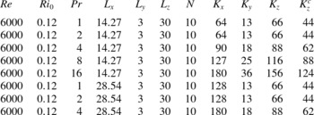
(rather than the whole domain), where presumably the most energetic turbulent activity occurs. For further discussion of this topic please refer to the supplementary data accompanying this paper, available at http://dx.doi.org/10.1017/jfm.2015.225. Table 1 summarizes the details of the set of different numerical experiments for which results will be presented below. The required extent of the computational domain has been chosen based on the previously described numerical analyses of Mashayek et al. (Reference Mashayek, Caulfield and Peltier2013) and Mashayek & Peltier (Reference Mashayek and Peltier2013). All of the analyses to be reported in this paper have been conducted at a fixed nominal initial Reynolds number of
 $\mathit{Re}=6000$
, which leads to a Taylor microscale Reynolds number of
 $\mathit{Re}_{{\it\lambda}}=O(10^{2})$
(see appendix A for further discussion) during the most intense phase of turbulence. At
 $\mathit{Pr}=1$
, an initial Reynolds number of
 $\mathit{Re}=6000$
has been shown to be high enough for mixing efficiency to remain unchanged for higher
 $\mathit{Re}$
and also to prohibit the pairing instability and the upscale cascade of energy which this vortex merger instability supports, as demonstrated in Mashayek & Peltier (Reference Mashayek and Peltier2013). This latter conclusion will be re-established in this paper to be as appropriate at high Prandtl number as it has been shown to be at
 $\mathit{Pr}=1$
. Thus for the primary mixing investigations, it will suffice to set the streamwise extent of our domain to include only a single wavelength (
 $L_{x}=14.27$
) of the fastest growing mode (FGM) of inviscid instability. In order to investigate the pairing instability, of course, we will set the streamwise extent to
 $2L_{x}$
. The most demanding simulation in the sequence that we will describe, that for
 $\mathit{Pr}=16$
, required approximately 5 701 632 core-hours on a BG/Q machine, which is approximately equivalent to a DNS study of a case with
 $\mathit{Pr}=1$
and
 $\mathit{Re}=40\,000$
, or
 $\mathit{Pr}=700$
and
 $\mathit{Re}=500$
(assuming the same numerical requirements concerning spatial resolution), all of which are unprecedented regimes that have not previously been investigated in the literature but which are highly relevant to the understanding of diapycnal mixing in the oceans.
Details of the three-dimensional numerical experiments in which the total grid points are about
 $N^{3}K_{x}K_{y}K_{z}$
. Also,
 $K_{z}^{c}$
represents the number of uniform elements resolving the innermost region of the domain in the vertical direction (
 $-5\leqslant z\leqslant 5$
).

In these simulations, flow evolution is initialized by adding a small two-dimensional perturbation in the form of the FGM of the Taylor–Goldstein equation (see e.g. Klaassen & Peltier Reference Klaassen and Peltier1985c
; Kundu & Cohen Reference Kundu and Cohen2008). The amplitude of this initial normal mode perturbation is set to 0.01, which translates into a kinetic energy of the seed two-dimensional disturbance that is
 $10^{-6}$
times smaller than the kinetic energy of the background flow. We also experimented with an alternative form for the initial perturbation with a shape function
 $\exp (-z^{2})$
, and discovered that while the results (including the shape of the billow and the sequence of secondary instabilities that arise) differ significantly at a low Reynolds number of
 $\mathit{Re}=750$
, they become noticeably insensitive to such choice of initial perturbation at sufficiently high
 $\mathit{Re}$
, which is the most relevant for the geophysical applications of interest to us. Thus at high
 $\mathit{Re}$
, the only difference incurred as a consequence of any such difference in the initialization procedure involves the computational time required to reach the saturation state for the initial KH billows, where our choice of FGM as the initial perturbation tends to minimize the required computational resources. In addition to the two-dimensional perturbation in the streamwise vertical plane (
 $x{-}z$
), it is absolutely critical to initially perturb the spanwise velocity with small-amplitude white noise in order for the three-dimensional instabilities to grow without bias from the initial conditions. The amplitude of such spanwise perturbations is set to 0.001, which translates into a level of three-dimensional disturbance that is initially one order of magnitude smaller than the two-dimensional disturbance. In the absence of such spanwise perturbation, the essential growth of three-dimensional instabilities would eventually be influenced by truncation errors at the grid scale and thus the flow field would become grid-dependent and hence physically implausible. Insofar as boundary conditions are concerned, the velocity and density fields are assumed to be periodic in both streamwise and spanwise directions, while the top and bottom boundaries are assumed to be free-slip and impermeable for velocity and insulated (zero density flux) for the density field.
2.3. Energetics and mixing analysis of three-dimensional DNS data
In order to analyse the flow energetics during the course of its evolution, we employ a Reynolds decomposition of the flow field into a mean (associated with the background flow) and perturbation components. Furthermore, the perturbation components of the velocity and density fields are themselves further subdivided into a spanwise averaged component associated with two-dimensional eddies (mainly associated with the initial KH wave) as well as an inherently three-dimensional component (Klaassen & Peltier Reference Klaassen and Peltier1991; Caulfield & Peltier Reference Caulfield and Peltier2000), expansions that we may write explicitly as
 $$\begin{eqnarray}\displaystyle & \boldsymbol{u}(x,y,z,t)=\overline{U}(z,t)+\boldsymbol{u}^{\prime }(x,y,z,t), & \displaystyle\end{eqnarray}$$
 $$\begin{eqnarray}\displaystyle & \boldsymbol{u}^{\prime }(x,y,z,t)=[u_{2d}+u_{3d},v_{3d},w_{2d}+w_{3d}], & \displaystyle\end{eqnarray}$$
 $2d$
) and three-dimensional (
 $3d$
) components, are defined by
 $$\begin{eqnarray}\displaystyle & \overline{U}(z,t)=\langle \boldsymbol{u}\rangle _{xy}, & \displaystyle\end{eqnarray}$$
 $$\begin{eqnarray}\displaystyle & (u_{2d},0,w_{2d})(x,z,t)=\langle (u-\overline{U},v,w)\rangle _{y}, & \displaystyle\end{eqnarray}$$
 $$\begin{eqnarray}\displaystyle & (u_{3d},v_{3d},w_{3d})(x,y,z,t)=(u-\overline{U}-u_{2d},v,w-w_{2d}) & \displaystyle\end{eqnarray}$$
 $\langle .\rangle _{p}$
denotes averaging in the
 $p$
direction).
An appropriate kinetic energy budget can be obtained by taking the inner product of (2.2) with the total velocity vector. The derivation is straightforward, and common in the derivation of turbulent balance equations (see e.g. Kundu & Cohen Reference Kundu and Cohen2008). The resulting evolution equation for the total kinetic energy
 $\mathscr{K}=\langle u^{2}+v^{2}+w^{2}\rangle _{xyz}/2$
becomes (Peltier & Caulfield Reference Peltier and Caulfield2003)
 $$\begin{eqnarray}\frac{\text{d}}{\text{d}t}\mathscr{K}=-\mathscr{H}+\mathscr{D}.\end{eqnarray}$$
The total kinetic energy in (2.11) is either transferred into buoyancy flux
 $\mathscr{H}$
, thereby increasing the potential energy of the system (i.e. it appears with a reversed sign in (2.15) below), or dissipated through viscous stresses at a rate
 $\mathscr{D}$
(which is negative definite), and these have the explicit definitions
 $$\begin{eqnarray}\displaystyle & \mathscr{H}=\mathit{Ri}_{0}\langle {\it\rho}w\rangle _{xyz}, & \displaystyle\end{eqnarray}$$
 $$\begin{eqnarray}\displaystyle & \mathscr{D}=\langle {\it\varepsilon}\rangle _{xyz}, & \displaystyle\end{eqnarray}$$
 ${\it\varepsilon}$
is the dimensionless viscous dissipation given by
 $$\begin{eqnarray}{\it\varepsilon}=-\frac{2}{\mathit{Re}}(\unicode[STIX]{x1D634}_{ij}\unicode[STIX]{x1D634}_{ij}),\end{eqnarray}$$
in which
 $\unicode[STIX]{x1D634}_{ij}=(\partial u_{i}/\partial x_{j}+\partial u_{j}/\partial x_{i})/2$
is the strain rate tensor.
The total averaged potential energy of the system, on the other hand, is defined as
 $\mathscr{P}=\mathit{Ri}_{0}\langle {\it\rho}z\rangle _{xyz}=\mathit{Ri}_{0}\langle z\overline{{\it\rho}}\rangle _{z}$
(Caulfield & Peltier Reference Caulfield and Peltier2000). Thus the time evolution of
 $\mathscr{P}$
is governed by the following evolution equation:
 $$\begin{eqnarray}\frac{\text{d}}{\text{d}t}\mathscr{P}=\mathscr{H}+\mathscr{D}_{p},\end{eqnarray}$$
where
 $\mathscr{H}$
is as defined in (2.12), and
 $\mathscr{D}_{p}$
represents the irreversible conversion of fluid internal energy into potential energy through the action of diffusive processes acting preferentially upon the smallest scales of the density heterogeneity in a statically stable, motionless environment, and is hence strictly positive. This contribution to the growth of potential energy may be approximated as (Caulfield & Peltier Reference Caulfield and Peltier2000)
 $$\begin{eqnarray}\mathscr{D}_{p}=\frac{\mathit{Ri}_{0}{\rm\Delta}{\it\rho}}{L_{z}\mathit{Re}\mathit{Pr}},\end{eqnarray}$$
where
 ${\rm\Delta}{\it\rho}$
is the density difference across the computational domain of height
 $L_{z}$
.
It is important to note that not all the exchange of energy between the kinetic and potential energy ‘reservoirs’ that occurs as a consequence of the action of the buoyancy flux
 $\mathscr{H}$
can be interpreted as irreversible mixing. In fact, this buoyancy flux is composed of two distinct components, the first of which we refer to as the stirring rate,
 $\mathscr{S}$
, and the second we identify as the mixing rate,
 $\mathscr{M}$
, which are associated with reversible and irreversible processes respectively. Such partitioning may be explicitly expressed as
 $$\begin{eqnarray}\mathscr{H}=\mathscr{M}+\mathscr{S}.\end{eqnarray}$$
This distinction between reversible stirring and irreversible mixing is fundamental to the original definition of available potential energy (APE) by Lorenz (Reference Lorenz1955), whose interest was in the application of this concept to the understanding of the general circulation of the atmosphere (see Peltier & Caulfield Reference Peltier and Caulfield2003 for a review). Following Winters et al. (Reference Winters, Lombard, Riley and D’Asaro1995) and Caulfield & Peltier (Reference Caulfield and Peltier2000), who applied this concept to the understanding of small-scale turbulent flows, one can subdivide the total averaged potential energy of the flow into APE, (
 $\mathscr{P}_{A}$
), and background potential energy or BPE, (
 $\mathscr{P}_{B}$
), by writing
 $$\begin{eqnarray}\mathscr{P}=\mathscr{P}_{A}+\mathscr{P}_{B}.\end{eqnarray}$$
In other words, at any instant of time in the course of flow evolution, the APE involved in reversible stirring of the turbulent flow is the difference between the actual potential energy of the flow field (
 $\mathscr{P}$
) and the notional statically stable background state (
 $\mathscr{P}_{B}$
). It follows from (2.15), (2.17) and (2.18) that the APE for ‘stirring’, which is available to be converted back into kinetic energy, evolves as
 $(\text{d}/\text{d}t)\mathscr{P}_{A}=\mathscr{S}=\mathscr{H}-\mathscr{M}$
and all the irreversible processes contribute to increase the background potential energy as
 $(\text{d}/\text{d}t)\mathscr{P}_{B}=\mathscr{M}+\mathscr{D}_{p}$
. So the amount of irreversible mixing is obtained from the background potential energy as
 $$\begin{eqnarray}\mathscr{M}=\frac{\text{d}}{\text{d}t}\mathscr{P}_{B}-\mathscr{D}_{p}.\end{eqnarray}$$
Here
 $\mathscr{P}_{B}=\mathit{Ri}_{0}\langle {\it\rho}_{B}z\rangle$
represents the minimum (background) average potential energy that would be obtained if the fluid flow were strictly statically stable with a mean background density profile of
 ${\it\rho}_{B}(z,t)$
. Finding
 ${\it\rho}_{B}(z,t)$
involves two steps: (i) adiabatic rearrangement of the fluid parcels according to their individual densities into a monotonically decreasing upwards assembly, and (ii) sequentially deforming the shape of individual fluid parcels and stacking them as individual isopycnal sheets in order to conserve mass (Winters et al.
Reference Winters, Lombard, Riley and D’Asaro1995; Caulfield & Peltier Reference Caulfield and Peltier2000). Such distortion, in our discretized space, converts a fluid parcel with mass
 ${\it\delta}m={\it\rho}{\it\delta}x{\it\delta}y{\it\delta}z$
into a sheet with thickness
 ${\it\delta}z_{B}={\it\delta}m/({\it\rho}_{B}L_{x}L_{y})$
.
Now the usual approach whereby this adiabatic rearrangement of the density field may be produced has been to numerically sort
 ${\it\rho}(x,y,z,t)$
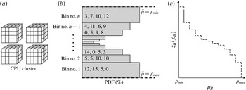
at every time step in the evolution of the flow (see for example Caulfield & Peltier Reference Caulfield and Peltier2000; Peltier & Caulfield Reference Peltier and Caulfield2003 and Mashayek & Peltier Reference Mashayek and Peltier2013). However, for large simulations such as those required for the purpose of the current study, such serial sorting algorithms become prohibitively expensive (or even impossible) to employ because of the computational time and memory requirements. An alternative and superior approach is one based on the use of probability density functions (PDFs), proposed by Tseng & Ferziger (Reference Tseng and Ferziger2001), which we have implemented for present purposes (for a simple MATLAB code illustrating this approach for a one-dimensional profile, see the supplementary data). The idea is to discretize the probability sample space of density
 $\tilde{{\it\rho}}$
into an appropriate number of a priori selected bins. The probability that
 ${\it\rho}(x,y,z,t)\in [\tilde{{\it\rho}},\tilde{{\it\rho}}+\text{d}\tilde{{\it\rho}}]$
can be defined as a volume integral of the delta function as
 $$\begin{eqnarray}\text{PDF}(\tilde{{\it\rho}})=\frac{1}{V}\int _{V}{\it\delta}(\tilde{{\it\rho}}-{\it\rho})\,\text{d}V.\end{eqnarray}$$
Once this PDF reference state has been constructed by scanning the entire domain, a corresponding reference distribution of height levels (
 $z_{B}$
) that is associated with a monotonically decreasing upwards density profile (
 ${\it\rho}_{B}$
) is obtained as (note that
 $L_{x}L_{y}{\it\delta}z_{B}=V\,\text{PDF}(\tilde{{\it\rho}})\,\text{d}\tilde{{\it\rho}}$
)
 $$\begin{eqnarray}z_{B}({\it\rho}_{B})=L_{z}\int _{{\it\rho}_{B}}^{{\it\rho}_{M}}\text{PDF}(\tilde{{\it\rho}})\,\text{d}\tilde{{\it\rho}}.\end{eqnarray}$$
Hence the background density profile (
 ${\it\rho}_{B}$
) is assumed constant between adjacent height levels (here
 ${\it\rho}_{M}$
denotes the maximum density). In order for this method to work properly, especially for high-gradient profiles such as
 $\tanh (z)$
, it is critical to employ a non-uniform mesh spacing in the sample space so as to concentrate the bins in regions with high density gradient. A Chebyshev transformation is therefore used in the present study, where the non-uniform spacing is calculated as
 $\text{d}\tilde{{\it\rho}}_{j}=\text{d}\tilde{{\it\rho}}_{u}\cos {\it\theta}_{j}$
, with
 $\text{d}\tilde{{\it\rho}}_{u}$
being the presumed uniform spacing and
 ${\it\theta}=0,\dots ,{\rm\pi}/2$
near both tails of
 $\tanh$
and
 ${\it\theta}=0,\dots ,{\rm\pi}$
in the central smoother region.
Figure 1 provides a schematic that illustrates the process of finding PDFs in a parallel computation. Having constructed a user-defined non-uniform distribution of bins (using a Chebyshev transformation) associated with a discretized probability sample space characterized by a monotonically decreasing upward assembly (figure 1 b), every computational core (depicted by gridded cubes in figure 1 a) searches among the grid elements under its control and assigns the density of each element to the appropriate bin of an a priori discretization in order to calculate the complete PDF using (2.20). Finally a global sum among all processors determines the total PDF in every bin, which is then interpolated to form the desired background density profile (figure 1 c).
Schematic illustration of a parallel computation of the sorted background density profile
 ${\it\rho}_{B}(z_{B})$
using the probability density functions as defined in (2.20) and (2.21). The numbers inside the bins in panel (b) are associated with each individual CPU of a cluster. The heights of the bins indicate the PDF (%) and their widths show the total thickness that is associated with the stacked layers of density that belong to that bin, i.e.
 ${\it\rho}(x,y,z,t)\in [\tilde{{\it\rho}},\tilde{{\it\rho}}+\text{d}\tilde{{\it\rho}}]$
.

Having isolated the amount of change in
 $\mathscr{P}$
that is associated with mixing through (2.18), one can calculate the mixing efficiency as proposed in Caulfield & Peltier (Reference Caulfield and Peltier2000). Combining (2.11) and (2.17), the rate of change of kinetic energy of the flow,
 $(\text{d}/\text{d}t)\mathscr{K}$
is controlled by stirring, mixing and viscous dissipation processes (
 $(\text{d}/\text{d}t)\mathscr{K}(t)=-\mathscr{S}-\mathscr{M}+\mathscr{D}$
), where the last two terms are irreversible. So the instantaneous efficiency of mixing
 $\mathscr{E}_{i}$
may be defined as the ratio of ‘useful’ expenditure of
 $\mathscr{K}$
to the total irreversible loss of
 $\mathscr{K}$
, i.e.
 $$\begin{eqnarray}\mathscr{E}_{i}=\frac{\mathscr{M}}{\mathscr{M}-\mathscr{D}}.\end{eqnarray}$$
3. Three-dimensional secondary stability analysis
The stratified shear flow with
 $\mathit{Ri}_{0}<1/4$
is susceptible to a two-dimensional primary instability in the form of a Kelvin–Helmholtz wave (when the shear layer is as thick as the density layer), which in turn undergoes secondary and higher-order instabilities (such as convective or Rayleigh–Taylor instability) that mediate the transition to turbulence and the transfer of shear flow kinetic energy into the background potential energy, hence mixing and entrainment. In order to understand the individual roles of the non-dimensional control parameters, such as the molecular Prandtl number, on the nature of turbulent mixing and the associated turbulent diffusivity of mass across isopycnals, one needs to first assess the role of each parameter in the nature of the different secondary instabilities that mediate the transition to turbulence (since this turbulence may retain a memory of the mechanism(s) of its production). In what follows, we employ an analytical method of linear non-separable stability analysis to predict the growth rates, spatial structures and dynamical origins of the secondary instabilities that govern the transition process. To facilitate the discussion we also employ a terminology that has become common in describing the anatomy of KH waves (e.g. Peltier & Caulfield Reference Peltier and Caulfield2003): in particular the word ‘eyelid(s)’ will be employed to denote the upper and lower peripheral regions of the vortex cores which are in turn connected to the adjacent billows by a strained vorticity filament that is referred to as the ‘braid’. In this discussion of the secondary instability activity, we will be focusing primarily upon the transition phase, during which the individual secondary instabilities are easily identifiable, a period including the time of saturation of the two-dimensional KH wave amplitude (denoted by
 $t_{2d}^{s}$
) but prior to its turbulent collapse.
3.1. Methodology
In this section we briefly describe the methodology for predicting the secondary modes of instability that grow on the background provided by the inherently two-dimensional KH wave (a non-parallel shear flow) when this is subjected to three-dimensional perturbations. This method was originally developed by Klaassen & Peltier (Reference Klaassen and Peltier1985c
) and has been employed previously for similar purposes (see e.g. Klaassen & Peltier Reference Klaassen and Peltier1991; Caulfield & Peltier Reference Caulfield and Peltier1994, Reference Caulfield and Peltier2000; Mashayek & Peltier Reference Mashayek and Peltier2012a
,Reference Mashayek and Peltier
b
). Four fundamental assumptions are involved in this methodology, which cast the stability analysis into the form of a standard matrix eigenvalue problem. First, the flow is assumed to be composed of a quasi-steady background component (which is two-dimensional and may be denoted by
 $\tilde{f}(x,z,t)$
), and an inherently three-dimensional perturbation component (
 $f^{\prime }(x,y,z,t)=f_{3d}(x,y,z,t)$
). Second, we further assume that both
 $\tilde{f}(x,z,t)$
and
 $f_{3d}(x,y,z,t)$
are periodic in the streamwise direction with a wavenumber
 ${\it\alpha}=2{\rm\pi}/L_{x}$
, where
 $L_{x}$
is the streamwise extent of the domain in which the two-dimensional KH wave has been numerically evolved and is chosen to be the wavelength of the most unstable mode of linear theory. Third, on the basis of Floquet theory, the perturbation field is also assumed to be periodic in the spanwise direction with a wavenumber
 $d$
and so may be assumed to take the form
 $f_{3d}(x,y,z,t)=f_{3d}^{\dagger }(x,z)\exp (\text{i}\,\text{d}y+{\it\sigma}_{3d}t)$
. Finally, we suppose that there exists a separation of time scales between the time rate of change of the background two-dimensional flow (as represented by a growth rate,
 ${\it\sigma}_{kh}$
) and that of possible three-dimensional secondary instabilities,
 ${\it\sigma}_{3d}$
, essentially assuming a steady state for the background flow (i.e.
 $\tilde{f}(x,z,t)=\tilde{f}(x,z)$
). Based on these assumptions, we can decompose the flow fields as follows:
 $$\begin{eqnarray}\displaystyle & f(x,y,z,t)=\tilde{f}(x,z)+f_{3d}(x,y,z,t), & \displaystyle\end{eqnarray}$$
 $$\begin{eqnarray}\displaystyle & f_{3d}(x,y,z,t)=f_{3d}^{\dagger }(x,z)\text{e}^{\text{i}\,\text{d}y+{\it\sigma}_{3d}t}, & \displaystyle\end{eqnarray}$$
 ${\it\sigma}_{3d}$
is the complex growth rate of an unstable mode. Notice that unlike our decomposition in (2.6) and (2.7) for diagnosing the three-dimensional DNS results, where we explicitly distinguished between the background parallel shear flow
 $\overline{U}$
and the non-parallel KH wave
 $u_{2d}$
, for the purpose of our secondary stability analysis the background state of the flow includes both of these components of the flow, i.e.
 $\tilde{u} (x,z,t)=\overline{U}(z,t)+u_{2d}(x,z,t)$
. The
 $3d$
notation, however, is unchanged here, and in both cases it represents the inherently three-dimensional components of the flow field.
Upon substitution of the above decomposition into (2.2)–(2.4) and linearizing about the two-dimensional background state, a set of perturbation equations are obtained for the velocity, density and pressure fields (
 $f_{3d}^{\dagger }(x,z)$
in (3.2) – see Klaassen & Peltier Reference Klaassen and Peltier1985c
for details). In order to recast the differential eigensystem into an algebraic eigenvalue problem, the perturbation fields
 $f_{3d}^{\dagger }(x,z)$
are discretized using a truncated set of orthogonal basis functions, i.e.
 $$\begin{eqnarray}\left.\begin{array}{@{}ll@{}}\displaystyle u_{3d}^{\dagger }=\mathop{\sum }_{{\it\lambda}=-L}^{L}\mathop{\sum }_{{\it\nu}=0}^{N}u_{{\it\lambda}{\it\nu}}F_{{\it\lambda}{\it\nu}},\quad & \displaystyle w_{3d}^{\dagger }=\mathop{\sum }_{{\it\lambda}=-L}^{L}\mathop{\sum }_{{\it\nu}=0}^{N}w_{{\it\lambda}{\it\nu}}G_{{\it\lambda}{\it\nu}},\\ \displaystyle {\it\rho}_{3d}^{\dagger }=\mathop{\sum }_{{\it\lambda}=-L}^{L}\mathop{\sum }_{{\it\nu}=0}^{N}{\it\rho}_{{\it\lambda}{\it\nu}}G_{{\it\lambda}{\it\nu}},\quad & \displaystyle p_{3d}^{\dagger }=\mathop{\sum }_{{\it\lambda}=-L}^{L}\mathop{\sum }_{{\it\nu}=0}^{N}p_{{\it\lambda}{\it\nu}}F_{{\it\lambda}{\it\nu}},\end{array}\right\}\end{eqnarray}$$
where
 $$\begin{eqnarray}F_{{\it\lambda}{\it\nu}}=\text{e}^{\text{i}{\it\lambda}{\it\alpha}x}\cos \frac{{\it\nu}{\rm\pi}z}{H},\quad G_{{\it\lambda}{\it\nu}}=\text{e}^{\text{i}{\it\lambda}{\it\alpha}x}\sin \frac{{\it\nu}{\rm\pi}z}{H}\end{eqnarray}$$
are the basis functions which are chosen in such a way as to satisfy Dirichlet and Neumann boundary conditions on their respective fields in (3.3) (i.e.
 $\partial _{z}F_{{\it\lambda}{\it\nu}}|_{z=0,H}=0$
and
 $G_{{\it\lambda}{\it\nu}}|_{z=0,H}=0$
where
 $H$
is the total height of the computational box).
Subsequently, by following the conventional Galerkin approach, the desired form of the eigenvalue problem is finally obtained by substituting the above expansions into the differential eigensystem and diagonalizing it by taking the appropriate inner products with
 $F_{{\it\lambda}{\it\nu}}^{\star }$
and
 $G_{{\it\lambda}{\it\nu}}^{\star }$
(where
 $\text{}^{\star }$
denotes complex conjugates). A symbolic representation of the eigenvalue problem so produced takes the form
 $$\begin{eqnarray}{\it\sigma}_{3d}V_{i}=\unicode[STIX]{x1D608}_{ij}V_{j},\end{eqnarray}$$
in which
 $\unicode[STIX]{x1D63C}$
is a constant matrix whose elements consist of complicated four-dimensional arrays (see the appendix of Smyth & Peltier Reference Smyth and Peltier1991 for their exact expressions) and
 $V$
is the concatenation of
 $\{u_{{\it\lambda}{\it\nu}},w_{{\it\lambda}{\it\nu}},{\it\rho}_{{\it\lambda}{\it\nu}}\}$
. The above matrix eigenvalue problem is then solved using conventional techniques.
We have employed the modified triangular truncation scheme of Klaassen & Peltier (Reference Klaassen and Peltier1985c
), namely
 $L({\it\nu})=[(N-{\it\nu})/2]$
in which square brackets represent ceiling integers and
 $N$
(an odd integer) is the truncation level which for practical reasons we chose to be
 $N=45$
, the highest truncation level we have yet to employ for the purpose of such analyses. Resolution studies have demonstrated the convergence in both growth rates and the structure of the eigenfunctions for all the modes that we will explicitly discuss below. In addition, the symmetries in the horizontal wavenumber space in the differential eigensystem requires the eigenvalues
 ${\it\sigma}_{3d}={\it\sigma}_{r}+\text{i}{\it\sigma}_{i}$
to be real (
 ${\it\sigma}_{i}=0$
) or to appear as a pair of complex conjugate modes. The latter represents two oppositely propagating waves, which taken together form a standing wave (Klaassen & Peltier Reference Klaassen and Peltier1985c
).
To gain further insight concerning the energy source of different modes of instability, an evolution equation for the growth rate of perturbation kinetic energy,
 ${\it\sigma}_{3d}=(d\mathscr{K}_{3d}/dt)/(2\mathscr{K}_{3d})$
where
 $\mathscr{K}_{3d}=\langle (|u_{3d}^{\dagger }|^{2}+|v_{3d}^{\dagger }|^{2}+|w_{3d}^{\dagger }|^{2})\rangle _{xz}/2$
, can be written as (Klaassen & Peltier Reference Klaassen and Peltier1991)
 $$\begin{eqnarray}\displaystyle & {\it\sigma}_{3d}=-\mathscr{H}_{3d}+\mathscr{S}h+\mathscr{S}t+\mathscr{D}_{3d}, & \displaystyle\end{eqnarray}$$
 $$\begin{eqnarray}\displaystyle & \mathscr{H}_{3d}=\mathit{Ri}_{0}\langle {\it\rho}_{3d}^{\dagger }w_{3d}^{\dagger }\rangle _{xz}/(2\mathscr{K}_{3d}), & \displaystyle\end{eqnarray}$$
 $$\begin{eqnarray}\displaystyle & \mathscr{S}h=-\langle (u_{3d}^{\dagger }w_{3d}^{\dagger })(\partial _{x}\tilde{w}+\partial _{z}\tilde{u} )\rangle _{xz}/(2\mathscr{K}_{3d}), & \displaystyle\end{eqnarray}$$
 $$\begin{eqnarray}\displaystyle & \mathscr{S}t=-{\textstyle \frac{1}{2}}\langle (|u_{3d}^{\dagger }|^{2}-|w_{3d}^{\dagger }|^{2})(\partial _{x}\tilde{u} -\partial _{z}\tilde{w})\rangle _{xz}/(2\mathscr{K}_{3d}), & \displaystyle\end{eqnarray}$$
 $$\begin{eqnarray}\displaystyle & \mathscr{D}_{3d}=\langle {\it\varepsilon}_{3d}^{\dagger }\rangle _{xz}/(2\mathscr{K}_{3d}), & \displaystyle\end{eqnarray}$$
 ${\it\varepsilon}_{3d}$
is as defined in (2.14) but for the perturbation velocity field.
Based on (3.6), the perturbation kinetic energy of a given mode may grow as a primary consequence of a number of different physical mechanisms. First, potential energy may be transferred into
 $\mathscr{K}_{3d}$
through convective instability of unstable density gradients as represented by perturbation buoyancy flux
 $\mathscr{H}_{3d}$
. Second,
 $\mathscr{K}_{3d}$
may be either produced or destroyed through ‘shear deformation’ by energy increase (or decrease) that occurs as a consequence of the interaction between the Reynolds stresses (
 $u_{3d}^{\dagger }w_{3d}^{\dagger }$
) and the background flow (both the parallel shear component and the non-parallel primary KH wave component) at a rate denoted by
 $\mathscr{S}h$
. Third, the kinetic energy of the secondary instability may grow or decay as a consequence of the action of the ‘strain deformation’ associated with the background flow acting upon individual fluid filaments (especially when the background includes significant anisotropy), the rate of which is represented by
 $\mathscr{S}t$
. Finally, a loss of
 $\mathscr{K}_{3d}$
may be caused by transformation into heat due to viscous dissipation, which is denoted in (3.6) by
 $\mathscr{D}_{3d}$
. Acceptable modes of secondary instability are associated with those solutions of (3.5) that not only ensure
 ${\it\sigma}_{3d}\gg {\it\sigma}_{kh}$
is satisfied (as required by our final fundamental assumption above), but also lead to closure of the perturbation kinetic energy budget (3.6).
3.2. Secondary instabilities
We have conducted our secondary stability analysis on a series of background non-parallel shear flows obtained using two-dimensional DNS simulations at
 $\mathit{Re}=6000$
,
 $\mathit{Ri}_{0}=0.12$
and
 $\mathit{Pr}=1,8,16$
. These background states included not only the initial parallel velocity shear flow, but also the rolled-up ‘spaghetti-on-a-fork-like’ density and vorticity fields of the KH wave component of the flow. Since the analysis assumes that the background state is frozen in time (i.e. quasi-steady assumption), we have performed this analysis for several snapshots in time about the saturation point of the primary KH wave. The selected times are ideally suited to the purpose of our stability analysis since the growth rate of three-dimensional perturbations during the saturation of the two-dimensional KH wave is much faster than that associated with the background state (i.e.
 ${\it\sigma}_{3d}=O(-1)\gg {\it\sigma}_{kh}=O(-4)$
), thus satisfying our fundamental assumption of time scale separation. Furthermore, inasmuch as the two-dimensional flow at this high
 $\mathit{Re}$
becomes turbulent even without adding the spanwise three-dimensional perturbations (unlike lower
 $\mathit{Re}$
experiments, which stay laminar in a two-dimensional setting and only become turbulent due to the added three-dimensional perturbations, as discussed in Klaassen & Peltier Reference Klaassen and Peltier1985b
), it is important to choose a limited range of time slices at which the background state has not undergone such unrealistic two-dimensional turbulence. The selected background states are proximate in time to the saturation time of the KH wave and so also satisfy the latter consideration.
This study extends the previous work of Mashayek & Peltier (Reference Mashayek and Peltier2012a
,Reference Mashayek and Peltier
b
) by exploring the stability of secondary modes at a higher Reynolds number for the background two-dimensional flows whose stability characteristics are to be investigated (their highest
 $\mathit{Re}$
was 2000) and, more significantly, by investigating the influence of elevating molecular Prandtl number above the value of unity. As a result of this shift in the region of parameter space of interest to us, and in particular due to a higher
 $\mathit{Re}$
, the conventional secondary instabilities studied so far will be seen to play more complicated roles in mediating the transition to turbulence, and to be modified importantly in terms of the physical mechanisms they represent. Understanding these differences in the operative secondary instabilities in the high-
 $\mathit{Re}$
, high-
 $\mathit{Pr}$
regime forms the main focus of this subsection. Besides the more conventional instabilities, we have also identified further inhabitants of the ‘zoo’ of such modes, but these will not be described here.
The conventionally understood secondary instabilities in the context of growing three-dimensional perturbations on a stratified KH wave include (i) the secondary shear-aligned convective instability (Klaassen & Peltier Reference Klaassen and Peltier1985c ) which produces shear-aligned streamwise vortex tubes of alternating sign in the spanwise direction in the billow eyelids, (ii) the secondary shear instability of the braid (manifested by inclined mini-replicas of the primary KH wave on the braid) originally discussed by Corcos & Sherman (Reference Corcos and Sherman1976), and (iii) the SPI (Mashayek & Peltier Reference Mashayek and Peltier2012a ) which is located at the stagnation point of the braid. In all the cases for which we have conducted non-separable stability analysis (for various selected times as well as the full bandwidth of the spanwise wavenumber), the SPI appeared to be the FGM with the secondary shear-aligned convective mode being next in the list, arranged in decreasing order of growth rate. Interestingly, the eigenfunction associated with the secondary shear instability on the braid does rise in prominence briefly as the FGM prior to its being replaced in that role by the SPI, and was never found to persist significantly in time. In the following subsections we will focus on the characteristics of these important instabilities in the parameter space of interest to us, by categorizing them into ‘braid instability’ and ‘eyelid instability’ types.
3.2.1. Braid instability
The SPI dominated the braid region in all of our two-dimensional simulations, while the shear instability on the braid did not emerge at
 $\mathit{Re}=6000$
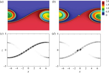
until the braid was perturbed by the surrounding instabilities at later times during flow evolution. Our secondary instability analysis also established similar results regarding the dominance of SPI, while the other braid instability could be most prominently realized at times prior to the actual emergence of SPI. Figure 2(a,b) illustrates the evolving two-dimensional background states before and after the emergence of SPI for a case with
 $\mathit{Pr}=1$
. Figure 2(c,d) depicts the eigenfunction associated with the perturbation kinetic energy of the FGM at these times. The eigenfunction at
 $t=64$
suggests KH-like vortices on the braid with strong perturbations along the braid representing the secondary shear instability. Nevertheless, at later times in the flow evolution this eigenfunction transitions into a more localized mode which is focused upon the stagnation point, and characterized by weaker perturbations (albeit non-zero) along the braid. As has been previously discussed in Mashayek & Peltier (Reference Mashayek and Peltier2012a
), the emergence of these two modes depends on the relative strength of the strain and shear fields when mapped into a braid-aligned coordinate system. For our
 $\mathit{Re}=6000$
analysis, the strength of the braid strain field must have initially overwhelmed velocity shear normal to the braid such that the secondary shear instability was inhibited and the SPI was dominant. With this view in mind, these two instabilities may be viewed simply as comprising two branches of the ‘braid instability’.
Demonstration of the braid instability (FGM) for
 $\mathit{Pr}=1$
at
 $t=64$
(a,c) and
 $t=70$
(b,d) corresponding to times before and after the emergence of SPI. (a,b) The density contour plots and (c,d) the perturbation kinetic energy eigenfunction that is associated with this mode of instability.

The competition between the shear and strain deformation fields on the braid is subtle. Based on an equilibrium similarity theory, Smyth (Reference Smyth2003) suggested that increasing
 $\mathit{Pr}$
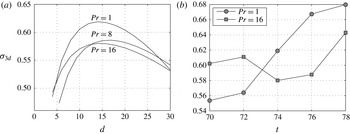
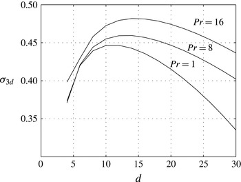
directly increases the shear across the braid-aligned coordinate system by further sharpening the density gradients. As will be discussed in the following section, the molecular Prandtl number also indirectly influences the strain field such that it suppresses the growth rate of SPI, resulting in a postponed emergence of this mode. Figure 3(a) plots the variation of growth rate
 ${\it\sigma}_{3d}$
with respect to spanwise wavenumber
 $d$
for
 $\mathit{Pr}=1,8,16$
obtained from a background state at the time of saturation of KH wave amplitude,
 $t_{2d}^{s}=74$
. As discussed by Mashayek & Peltier (Reference Mashayek and Peltier2012a
) and also shown in this figure, this mode is highly three-dimensional as it exists at a wide range of cross-stream wavelengths, unlike the shear instability on the braid which is primarily two-dimensional. Moreover, at this time, the growth rate associated with SPI decreases at almost all wavelengths as
 $\mathit{Pr}$
increases. In order to fully assess the suppression of SPI due to higher
 $\mathit{Pr}$
, figure 3(b) compares the time variation of
 ${\it\sigma}_{FGM}$
associated with the wavenumber of maximum growth rate for
 $\mathit{Pr}=1$
and
 $\mathit{Pr}=16$
. This plot suggests that for
 $\mathit{Pr}=1$
the highest growth rate is sustained for a longer period of time, whereas for
 $\mathit{Pr}=16$
,
 ${\it\sigma}_{FGM}$
reaches similar rates only briefly. Since SPI extracts its energy from the strain deformation field of the braid, its suppression due to higher
 $\mathit{Pr}$
must have been caused by weakening of this field. As will be suggested in the next section, the strain and shear fields are indirectly influenced by
 $\mathit{Pr}$
due to the promotion of the ‘eyelid instability’, which modifies these fields in such a way that the emergence of SPI is postponed. We will also confirm the suppression of SPI due to an increase in the molecular Prandtl number based on our three-dimensional DNS results below.
The suppression of SPI due to higher
 $\mathit{Pr}$
at a fixed
 $\mathit{Re}$
and
 $\mathit{Ri}$
. (a) The variation of growth rate
 ${\it\sigma}_{3d}$
associated with FGM at
 $t_{2d}^{s}$
for the full bandwidth of spanwise wavenumbers. (b) Time variation of
 ${\it\sigma}_{3d}$
at the wavenumber associated with its maximum rate.

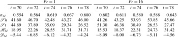
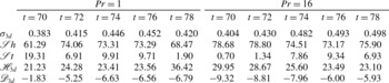
Table 2 summarizes the growth rates associated with SPI at the spanwise wavenumber of maximum growth rate for
 $\mathit{Pr}=1$
and
 $\mathit{Pr}=16$
. Moreover, the energetic contribution of different mechanisms to the growth of perturbation kinetic energy as introduced in (3.6) is also reported as a percentage in this table. Notice that the share of
 $\mathscr{H}_{3d}$
increases monotonically in time for all
 $\mathit{Pr}$
, highlighting the three-dimensional nature of this mode of instability, which is enhanced in the course of flow evolution.
The growth rate
 ${\it\sigma}_{3d}$
and energetic properties (in percentage and as introduced in (3.6)) of the most unstable three-dimensional mode associated with the SPI.

3.2.2. Eyelid instability
In all our two-dimensional simulations the secondary shear-aligned convective instability dominated the billow eyelid (as opposed to the braid). Besides the conventional picture for this mode, which consists of a periodic array of streamwise vortices in the spanwise direction and are convectively driven, we have discovered a new characteristic associated with this mode of instability at high Reynolds and Prandtl number, consisting of spanwise vortices that are counter-rotating in the vertical direction and are shear-driven. The latter property for this mode is new and has not been realized in the previously published literature on the stability analysis of these secondary modes, primarily due to the much lower values of
 $\mathit{Re}$
at which these previous analyses have been performed. This new characteristic prompts us to refer to this mode simply as an ‘eyelid instability’. In this section, we will first analyse the impact of
 $\mathit{Pr}$
on the convectively driven component of the instability by investigating its influence on the Rayleigh number of the most statically unstable region of the billow. We will then explain the shear-driven counter-rotating vortex component of the mode that seems to follow the development of the convectively driven component and eventually appears most prominently around the diagonal corners of the eyelid(s). Finally in this section we will address the critical role of
 $\mathit{Pr}$
in transforming this mode into a short-wave instability, capable of directly injecting turbulence into small scales.
The contour plots of buoyancy frequency
 $N^{2}$
for (a)
 $\mathit{Pr}=1$
and (b)
 $\mathit{Pr}=16$
at
 $t_{2d}^{s}$
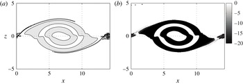
in which the shaded regions illustrate the statically unstable SARs in which
 $N^{2}<0$
.

Figure 4 illustrates the buoyancy frequency contours associated with
 $\mathit{Pr}=1$
and
 $\mathit{Pr}=16$
at
 $t_{2d}^{s}$
. The super adiabatic regions (SARs) in which the density distribution is statically unstable are shaded in this figure. As shown in this plot, the degree of static instability associated with these regions is enhanced as
 $\mathit{Pr}$
increases, which is mainly a consequence of a higher density gradient across the SARs. This is because the decreased density diffusion inside the core at higher values of
 $\mathit{Pr}$
tends to only weakly thin the SAR but to significantly increase the density contrast across it (Klaassen & Peltier Reference Klaassen and Peltier1985a
). In analogy with the Rayleigh–Bénard problem, we define a Rayleigh number representative of the outermost statically unstable region that is most likely to exceed the critical value (which is usually of order
 $10^{3}$
) for the onset of convective instability (Klaassen & Peltier Reference Klaassen and Peltier1985c
) as
 $$\begin{eqnarray}\mathit{Ra}=\mathit{Re}^{2}\,\mathit{Ri}\,\mathit{Pr}\,{\rm\Delta}{\it\rho}^{\star }{\it\delta}^{3},\end{eqnarray}$$
where
 ${\rm\Delta}{\it\rho}^{\star }$
represents the dimensionless density contrast across the outermost SAR and
 ${\it\delta}$
is its dimensionless thickness. This expression might suggest that
 $\mathit{Ra}\propto \mathit{Pr}$
. However, as mentioned earlier,
 ${\rm\Delta}{\it\rho}^{\star }$
and
 ${\it\delta}$
are both functions of
 $\mathit{Pr}$
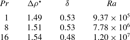
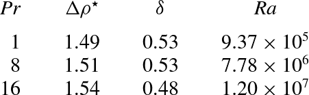
, and for a fluid with higher molecular Prandtl number they have opposing effects on the Rayleigh number. In order to understand these intricate connections, table 3 contains the measured values of
 ${\rm\Delta}{\it\rho}^{\star }$
and
 ${\it\delta}$
for a vertical profile in the middle of the billow as well as the calculated Rayleigh number using (3.11). As expected
 ${\rm\Delta}{\it\rho}^{\star }$
increases for higher
 $\mathit{Pr}$
, primarily due to reduced density diffusion inside the billow core at the bottom edge of the SAR, while the density at the upper edge remains unchanged as
 $\mathit{Pr}$
increases. Moreover,
 ${\it\delta}$
decreases for higher
 $\mathit{Pr}$
. Overall the Rayleigh number increases monotonically but not linearly with the Prandtl number, and we can conclude that the indirect impact of
 $\mathit{Pr}$
on
 $\mathit{Ra}$
via both
 ${\rm\Delta}{\it\rho}^{\star }$
and
 ${\it\delta}$
is of second order while its direct impact on
 $\mathit{Ra}$
through (3.11) (i.e.
 $\mathit{Ra}\propto \mathit{Pr}$
or lower molecular diffusivity is associated with higher Prandtl numbers and thus higher Rayleigh numbers) is of first order.
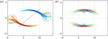
Illustrations of the different components of the eigenfunction associated with the eyelid instability. (a) Perturbation streamwise vorticity,
 ${\it\omega}_{3d}^{\dagger }|_{x}$
, associated with the convectively driven counter-rotating streamwise vorticity component of the mode. (b) Perturbation spanwise vorticity,
 ${\it\omega}_{3d}^{\dagger }|_{y}$
, associated with the shear-driven counter-rotating spanwise vorticity component of the ‘eyelid’ mode.

The measured values of density contrast across the SAR (
 ${\rm\Delta}{\it\rho}^{\star }$
) and the thickness of the SAR (
 ${\it\delta}$
) as well as the calculated Rayleigh number
 $\mathit{Ra}$
(3.11) for a vertical profile in the middle of the billow.
A new property of the eyelid instability at high
 $\mathit{Re}$
which was discovered through our non-separable stability analysis is that the usual low-
 $\mathit{Re}$
convectively driven instability is transformed into a mixed shear/convection-driven mode. Figure 5 illustrates different characteristics of the eigenfunction associated with this mixed mode. Figure 5(a) depicts the perturbation streamwise vorticity component thus corresponding to the convectively driven aspect of the eyelid instability. This perturbation, if it were to grow in isolation, would have the form of counter-rotating vortex tubes that are periodic in the cross-stream spanwise direction and aligned by the shear. Notice in this figure that the convective component of this instability contains noticeable perturbations that are inclined towards the diagonal edges of the billow in the shear direction, as indicated by a dashed line.
In addition, figure 5(b) illustrates the perturbation spanwise vorticity component of the same eigenfunction, thus corresponding with the shear component of the eyelid instability. If it were to develop in isolation, this perturbation would be manifested as counter-rotating vortices in the streamwise vertical
 $x{-}z$
plane (notice the positive and negative vorticity regions in the eyelid) wrapped around the core. The required shear for the existence of these counter-rotating spanwise vortices is created due to the KH roll-up process, during which fluid regions characterized by different streamwise velocities become superimposed and produce alternately retrograde and prograde ‘jets’. At high
 $\mathit{Re}$
the shear becomes sufficiently strong that this component of the vorticity eigenfunction strongly emerges. In fact, the convective and shear components of the eyelid instability are dynamically coupled. The convectively driven streamwise vortex tubes modulate the jet, which is formed by the fluid entering the eyelid, in such a way that the jet becomes alternately compressed (hence strengthened) and expanded (hence weakened). The strengthening and weakening of the jet in turn modulates the shear, which induces counter-rotating spanwise vortices associated with the shear-driven component of the eyelid instability. It is also important to note that the shear-driven component of the eyelid instability was also apparent in the high-
 $\mathit{Re}$
DNS results of Mashayek & Peltier (Reference Mashayek and Peltier2013); however, in Mashayek & Peltier (Reference Mashayek and Peltier2012a
) (see their figure 16) it was plausibly but incorrectly attributed to an extension of the secondary shear instability on the braid into the eyelid region. We will confirm the emergence of both properties of the eyelid instability in our three-dimensional DNS results, which will be discussed below.
The fluid’s Prandtl number plays a primary role in the growth of the eyelid instability, while its influence on the braid instabilities is only secondary through possible modification of the shear (Smyth Reference Smyth2003) and strain fields around the braid. The indirect impact of
 $\mathit{Pr}$
on the SPI, which was noted earlier in § 3.2.1, can be recognized by inspection of figure 5(a), where the convectively driven perturbations extend to regions surrounding the stagnation point (shown by dashed circles in this figure), which might modify the shear and strain fields of the braid such that at higher
 $\mathit{Pr}$
the onset of SPI is postponed. This expected impact will be fully verified in our three-dimensional DNS results, to be discussed in the next section. On the other hand, changing
 $\mathit{Pr}$
affects the eyelid instability dramatically. We discussed earlier the role of increasing
 $\mathit{Pr}$
on
 $\mathit{Ra}$
and hence intensification of the convective forcing of this mode of secondary instability. Furthermore, the shear-driven component of this mode is also promoted as
 $\mathit{Pr}$
increases (due to the dynamic coupling explained earlier) such that the counter-rotating vortices grow in abundance, appearing first as KH-like vortices on the top and bottom peripheries which propagate along the shear direction and later populate the diagonal corners (in the shear direction) of the eyelid.
Similar to table 2, table 4 includes the growth rate as well as the detailed energetic information associated with the eyelid instability during different times for
 $\mathit{Pr}=1$
and
 $\mathit{Pr}=16$
. Notice that irrespective of
 $\mathit{Pr}$
, the shear contribution (
 $\mathscr{S}h$
) to the growth rate of perturbation kinetic energy is always approximately 70–80 %, while convection (
 $\mathscr{H}_{3d}$
) has a 20–30 % share in the growth rate of the eyelid instability at our choice of
 $\mathit{Re}$
and
 $\mathit{Ri}_{0}$
. We also expect the convectively driven component of the eyelid instability to precede the shear-driven component and therefore be manifested earlier, simply because for earlier times during the growth of three-dimensional perturbations (not shown in this table) the relative contribution of convection to shear (
 $\mathscr{H}_{3d}/\mathscr{S}h$
) increases.
Similar to figure 3(a), which showed the persistence of SPI throughout the entire bandwidth of the spanwise wavenumber, figure 6 plots the growth rate of the eyelid instability (second FGM) at
 $t_{2d}^{s}$
for various spanwise wavenumbers and for
 $\mathit{Pr}=1,8,16$
. In general due to a higher
 $\mathit{Re}$
, the eyelid instability is active at shorter wavelengths as noted by Mashayek & Peltier (Reference Mashayek and Peltier2012a
). Nevertheless, as shown in figure 6, by increasing
 $\mathit{Pr}$
the wavenumber associated with the highest growth rate also increases, which implies a length scale contraction associated with this secondary mode of instability. In particular, note the significant increase of the growth rates of the shortest wavelengths which tends to flatten the growth rate versus cross-stream wavenumber curve. Unlike lower-
 $\mathit{Re}$
simulations (at
 $\mathit{Pr}=1$
) in which there exists a distinct wavenumber at which the growth rate becomes maximum (
 $d\approx 3{-}4$
) (see e.g. Caulfield & Peltier Reference Caulfield and Peltier2000), in our simulations with a much higher
 $\mathit{Re}$
and
 $\mathit{Pr}$
, a preferred wavelength ceases to exist as the curve becomes increasingly flat at short wavelengths as
 $\mathit{Pr}$
increases, suggesting that in the limit of extremely high
 $\mathit{Pr}$
there would be no wavenumber selectivity at all. This fundamental modification of length scales at higher
 $\mathit{Pr}$
suggests that the ‘eyelid instability’ is capable of directly injecting turbulence into all scales of motion. We will further discuss this topic in the next sections using three-dimensional DNS results.
The variation of perturbation growth rate
 ${\it\sigma}_{3d}$
at
 $t_{2d}^{s}$
associated with the eyelid instability (second FGM) for
 $\mathit{Pr}=1,8,16$
for the full bandwidth of spanwise wavenumbers
 $d$
.

Similar to table 2 but for the second most unstable three-dimensional mode associated with the eyelid instability.

4. Three-dimensional simulations
In this section we first explore different phases of flow evolution, including some preliminary observations obtained from the evolution of the kinetic energy reservoirs. We then focus again on the transition phase and further investigate the characteristics of secondary instabilities as revealed in the results of our three-dimensional numerical simulations, in order to confirm our findings concerning the impact of elevated
 $\mathit{Pr}$
on their growth rates, scale and dimensionality.
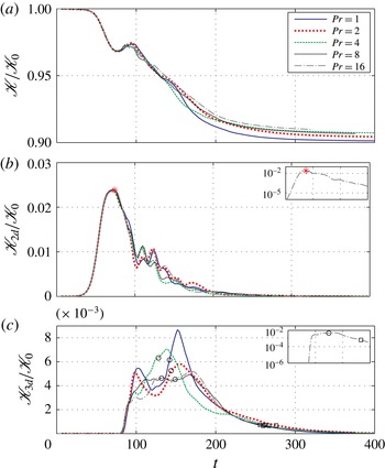
Time evolution of total kinetic energy (a) as well as its subdivisions into kinetic energy associated with two-dimensional KH roll-up (b) and the kinetic energy of the inherently three-dimensional perturbations (c), after being normalized by the initial value of the total kinetic energy denoted by
 $\mathscr{K}_{0}$
. The insets in (b) and (c) provide a broader picture in a log-scale only for
 $Pr=16$
. The saturation point of
 $\mathscr{K}_{2d}$
in (b) is marked with an asterisk. The three phases of flow evolution are separated in (c) by
 $t_{f}^{o}$
(circle) and
 $t_{f}^{e}$
(square).

4.1. The phases of turbulent flow evolution
By employing the velocity decomposition in (2.6) and (2.7), the total kinetic energy budget of the flow can also be decomposed as
 $\mathscr{K}=\overline{\mathscr{K}}+\mathscr{K}_{2d}+\mathscr{K}_{3d}$
. In figure 7, we plot the time variation of the reservoir of total kinetic energy
 $\mathscr{K}$
as well as that of two of its individual components associated respectively with the kinetic energy of the spanwise averaged motions
 $\mathscr{K}_{2d}$
and the kinetic energy of the three-dimensional ‘turbulence’
 $\mathscr{K}_{3d}$
. It proves useful at this point to characterize the life cycle of shear layer evolution as involving three primary phases, namely (I) the initial growth phase, (II) the fully turbulent regime, and (III) the final decay regime.
(I) The initial growth phase coincides with the growth of the primary two-dimensional KH instability as well as the secondary (or indeed tertiary) instabilities, catalysed from the initial laminar shear flow with initial minimum gradient Richardson number
 $\mathit{Ri}_{0}$
below the Miles–Howard critical value of
 $\mathit{Ri}=0.25$
. For all of the analyses to be discussed in this paper we have fixed the properties of the initial parallel flow to be characterized by
 $\mathit{Ri}_{0}=0.12$
, a value that is slightly below the Richardson number found to be maximally efficient for mixing at
 $\mathit{Pr}=1$
in the analyses of Mashayek et al. (Reference Mashayek, Caulfield and Peltier2013). In this initial phase of flow evolution the amplitude of the two-dimensional finite amplitude billow saturates at a time denoted by
 $t_{2d}^{s}$
in the previous section (the time of the maximum in the
 $\mathscr{K}_{2d}$
time series). Following the saturation of
 $\mathscr{K}_{2d}$
, as is evident from figure 7, the growth of intrinsically three-dimensional fluctuations commences, characterized by an abrupt rise in
 $\mathscr{K}_{3d}$
, leading eventually to complete turbulent collapse of the density stratified shear flow. Such fast growth of
 $\mathscr{K}_{3d}$
confirms the separation of time scales between the growth rate of primary two-dimensional KH instability and the secondary three-dimensional instabilities, which is an essential condition underlying the validity of our non-separable linear stability analysis as discussed in § 3.1.
A second phase of flow evolution is the fully turbulent regime (II), during which the most energetic small-scale turbulent motions exist and the associated three-dimensional perturbations themselves saturate. The onset of this phase, identified as
 $t_{f}^{o}$
, can be characterized by the time at which
 $\mathscr{K}_{3d}$
overwhelms
 $\mathscr{K}_{2d}$
, which occurs after the full collapse of the KH wave into turbulence. The sustained turbulent phase of flow evolution continues until a time denoted by
 $t_{f}^{e}$
at which the buoyancy Reynolds number
 $\mathit{Re}_{b}=|\mathscr{D}|/({\it\nu}\langle N^{2}\rangle _{z})$
(which is a dimensionless measure of turbulent intensity) reaches a critical value, usually taken to be approximately
 $\mathit{Re}_{b}=20$
(Stillinger, Helland & van Atta Reference Stillinger, Helland and van Atta1983; Smyth & Moum Reference Smyth and Moum2000b
) representing a lower limit below which stratification would be expected to suppress turbulent activity. Our DNS results during this phase correspond to
 $20<\mathit{Re}_{b}<150{-}250$
, which reaches the respective range of
 $\mathit{Re}_{b}=O(10{-}10^{4})$
that is commonly associated with oceanographic observations (e.g. Smyth et al.
Reference Smyth, Moum and Caldwell2001; van Haren & Gostiaux Reference van Haren and Gostiaux2010).
The final phase of flow evolution is associated with the final decay regime (III), during which the most intense turbulence of the second phase gradually decays, eventually leading to a complete re-laminarization of the flow and the return to a new state of stratified parallel flow, which again might be unstable to small-amplitude perturbations according to the Miles–Howard criterion, provided that further sufficiently strong shear were applied. As a consequence of the mixing that has occurred during the evolution of the turbulent flow, the initial shear layer has thickened and a substantial conversion of initial kinetic energy into potential energy has occurred.
We next focus upon the effects of changing molecular Prandtl number while keeping other non-dimensional control parameters fixed at
 $\mathit{Re}=6000$
and
 $\mathit{Ri}_{0}=0.12$
. Figure 7 demonstrates that the two-dimensional KH billow saturates at a time that is essentially independent of
 $\mathit{Pr}$
, and hence
 $t_{2d}^{s}$
is almost identical in all cases. In other words, the differences between the molecular diffusion rates for momentum and density are overwhelmed by the faster growth rates of the primary KH instability, and thus
 $\mathit{Pr}$
has a negligible impact on
 $\mathscr{K}_{2d}$
during the initial growth phase prior to
 $t_{2d}^{s}$
. In contrast, insofar as the abrupt growth of the three-dimensional secondary instabilities is concerned,
 $\mathit{Pr}$
plays a key role due to its influence on emergence, abundance and growth rate of the secondary instabilities that were discussed in depth in § 3.2, and hence the time series associated with the total kinetic energy and its individual components undergo complex variations. We will reassess the impact of
 $\mathit{Pr}$
on these instabilities and the associated mixing they engender in the following subsections, but here we will first focus on a number of additional characteristics of these phases of flow development.
First, prior to
 $t_{2d}^{s}$
, two-dimensional KH billows are energized by the background shear flow, but at a time subsequent to
 $t_{2d}^{s}~(t\approx 75{-}100)$
,
 $\mathscr{K}_{2d}$
drops, which corresponds to a transfer of energy from the two-dimensional KH wave to the background mean flow and hence to the development of a local maximum in all the time series describing the evolution of
 $\mathscr{K}$
. In addition, this loss in
 $\mathscr{K}_{2d}$
also provides the energy for the growth of secondary instabilities (see the abrupt rise in
 $\mathscr{K}_{3d}$
). Such extraction of kinetic energy from the two-dimensional KH billow becomes less intense as
 $\mathit{Pr}$
increases (notice the suppression of the local maximum in
 $\mathscr{K}$
that occurs in the range
 $t\approx 90{-}100$
). The subsequent drop in
 $\mathscr{K}$
, following the collapse of the original two-dimensional KH billow, is associated with the most intense mixing activity that develops during flow evolution (as will be discussed in detail below) and which results in the transfer of kinetic energy into background potential energy more efficiently than during the sustained turbulent phase.
Second, at low
 $\mathit{Pr}$
and during the transition to the fully turbulent regime,
 $\mathscr{K}_{3d}$
has a pronounced double-peak structure, indicating the occurrence of successive periods of gain and loss of turbulent kinetic energy which is associated with concurrent oscillations of
 $\mathscr{K}_{2d}$
, suggesting that there is a tendency for three-dimensional flow to retain some portion of its initial two-dimensionality immediately after the KH billow collapses, especially at
 $\mathit{Pr}=1$
and
 $\mathit{Pr}=2$
(i.e. the turbulent flow is more anisotropic in these cases). However, this tendency appears to be markedly reduced at higher
 $\mathit{Pr}$
, suggesting that the fully turbulent phase becomes more isotropic as
 $\mathit{Pr}$
increases. The first of these two successive extrema (more noticeable for the
 $\mathit{Pr}=1$
and
 $\mathit{Pr}=2$
cases) occurs near
 $t\approx 100$
subsequent to the collapse of the KH billow, indicating that the three-dimensional turbulence benefits from such transfer of the APE (that had built up during the KH roll-up) into the background potential energy reservoir. However, such transfer from
 $\mathscr{K}_{2d}$
to
 $\mathscr{K}_{3d}$
diminishes at higher
 $\mathit{Pr}$
, as shown by a marked reduction in
 $\mathscr{K}_{2d}$
and similarly the reduced gain in
 $\mathscr{K}_{3d}$
, which is eventually manifested in the disappearance of the first local maximum peak in
 $\mathscr{K}_{3d}$
for the higher
 $\mathit{Pr}$
cases. This suggests that the secondary instabilities, which extract their energy for growth from the two-dimensional KH wave, become less ‘effective’ as
 $\mathit{Pr}$
increases. However, it is interesting to note that the apparent ineffectiveness of the secondary instabilities for higher
 $\mathit{Pr}$
leads to a more isotropic distribution of energy, one in which
 $\mathscr{K}_{2d}$
does not regain its energy content (i.e. no rise in
 $\mathscr{K}_{2d}$
following the initial increase of three-dimensionality) after the initial transfer into
 $\mathscr{K}_{3d}$
. The fact that an increase in molecular
 $\mathit{Pr}$
supports a more isotropic turbulent state is in accord with previous findings in the literature (see e.g. Smyth & Moum Reference Smyth and Moum2000a
). We will return to the underlying physical reason behind this in § 4.3 and discuss its connection with the apparent role of
 $\mathit{Pr}$
in rendering the secondary instabilities less ‘effective’.
A third observation that follows from the results of the analyses documented in figure 7 focuses once more on the properties of the fully turbulent regime, during which the turbulence seems to become increasingly stationary as
 $\mathit{Pr}$
increases. This is clearly evident on the basis of the almost uniform, time-independent variation of
 $\mathscr{K}_{3d}$
at high
 $\mathit{Pr}$
(note especially the results for
 $\mathit{Pr}=8$
and
 $\mathit{Pr}=16$
), during which even the second peak of the former double-peak structure (which is still apparent at
 $\mathit{Pr}=4$
) is essentially eliminated. As a consequence of this sustained period of stationary turbulent flow at high
 $\mathit{Pr}$
, the fully turbulent regime reaches the saturation state much earlier as turbulent evolution of the flow continues, although the maximum intensity of turbulent activity is diminished.
Our final observation in this section focuses on the total loss in kinetic energy as can be observed from the time series of
 $\mathscr{K}$
. During the course of turbulent evolution from the initial stratified shear flow, the molecular
 $\mathit{Pr}$
does impact the total loss in the initial kinetic energy and hence is expected to show a similar trend in the increase of the background potential energy, associated with the total entrainment of the ambient fluid into the mixing layer. More precisely, as
 $\mathit{Pr}$
increases, the total loss of kinetic energy and the associated rise in the background potential energy decrease, implying a less vigorous entrainment of fluid into the mixing layer from the flanks of the shear flow where the ambient speed is highest. We will return to the above preliminary observations after analysing in detail the impacts of the molecular Prandtl number on secondary instabilities and the mixing that ensues. These will be the foci of the following sections.
4.2. Visualizations of secondary instabilities growing on the primary Kelvin–Helmholtz billows
Figure 8 illustrates the three-dimensional structures associated with the important eyelid instability for various values of
 $\mathit{Pr}$
and at several time instants during the initial growth phase. In this figure, at the time when the two-dimensional flow associated with the main KH wave saturates (i.e. at
 $t_{2d}^{s}=72{-}74$
), the convectively driven component of this instability (the so-called shear-aligned convective instability) emerges as streamwise vorticity tubes (e.g. shown for
 ${\it\omega}_{x}=\pm 0.01$
) with negative and positive signs. These vortex tubes form clear convective cells which locally overturn the statically unstable fluid that forms in the eyelids of the billows during roll-up. Comparing the structure of these vortex tubes for different
 $\mathit{Pr}$
at
 $t_{2d}^{s}$
demonstrates the development of an increasing number of shear-aligned convective rolls in the cross-stream direction as
 $\mathit{Pr}$
increases and thus a decrease in their characteristic cross-stream wavelength. This is completely in accord with our analytical findings in § 3.2 regarding the effect of higher
 $\mathit{Pr}$
in shifting the maximum growth rates towards higher wavenumbers (see figure 6) leading to length scale contraction. Furthermore, note that at any spanwise cross-section, the convective rolls possess opposite signs, again in accord with our prediction in figure 5(a).
Iso-surfaces of
 ${\it\omega}_{x}=\pm 0.01$
at various
 $\mathit{Pr}$
showing the growth of shear-aligned secondary convective instability, manifested as vortex tubes with alternating signs peripheral to the billow core.

Contour plots of spanwise vorticity
 ${\it\omega}_{y}$
at the mid-point in the cross-stream
 $y$
direction, demonstrating the growth of both types of braid instability: shear instability on the braid and SPI for various
 $\mathit{Pr}$
.

At a later time (
 $t=80$
), the other component of the eyelid instability is seen to develop on the initially dominant shear-aligned convective rolls, which is manifested in the form of small-scale spanwise vortices, which were also predicted for this region based upon our linear secondary instability theory of the previous section – a characteristic of this instability that is inherently shear-driven, not convectively driven. These vortices then travel in the shear direction and are eventually obscured by the complete turbulent collapse of the flow, during which evidence also appears of the action of tertiary Rayleigh–Taylor instability, which can be recognized at
 $t=82$
in the region surrounding the eyelids, for example. Meanwhile, as the secondary convective instability perturbs the eyelid region, the SPI dominates the action in the central portion of the braid with a spanwise wavenumber similar to that of the eyelid instability (also shown in figure 8).
The growth of the secondary shear-driven instabilities (either on the braid or the eyelid region of the billow) can be better captured in a streamwise vertical (
 $x{-}z$
plane) illustration of the spanwise vorticity. Figure 9, illustrates contours of spanwise vorticity at the mid-point in the cross-stream
 $y$
direction, during the same phase of the KH cycle, a time period after the saturation of the KH billow and before its full collapse into turbulence. Notice in this figure that the stagnant core associated with the SPI mode reduces in size, implying its suppression at higher
 $\mathit{Pr}$
in agreement with our analytical findings in the previous section. Moreover, the spanwise structure associated with this unstable mode resembles that of the shear-aligned convective rolls (as shown in figure 8); this may be understood after recalling the contribution of
 $\mathscr{H}_{3d}$
to the energetics of the SPI mode as noted in table 2. As the sequence of plots at different
 $\mathit{Pr}$
in figure 9 shows, secondary shear instabilities of the braid vorticity emerge after both shear-aligned convective instability and SPI and are excited by perturbations induced by the stagnant vortex core or extensions of the convective instability near the braid (see for example figure 9,
 $t=82$
at
 $\mathit{Pr}=1$
). Nevertheless, comparing the number of such vortex cores along the braid at
 $t=82$
for all
 $\mathit{Pr}$
, suggests that the induced shear instability on the braid tends to be promoted as
 $\mathit{Pr}$
increases. This can be explained by recalling the direct influence of
 $\mathit{Pr}$
in sharpening the density gradients across the braid (Smyth Reference Smyth2003) as well as the indirect influence of
 $\mathit{Pr}$
through the suppression of SPI at higher
 $\mathit{Pr}$
, which has to do with the weakening of the braid strain field (see figure 3). As a consequence, braid shear dominates, leading to the emergence of secondary shear instability on the braid. Note that the eigenfunction associated with the braid instability already supports the potential growth of these perturbations (albeit weakly), as shown in figure 2.
A critical observation from figure 9 involves identification of the shear-driven component of the eyelid instability. Notice in this figure the counter-rotating shear instabilities that first appear on the top and bottom of the eyelid and then grow both in size and abundance as they travel in the shear direction. This instability leads to a core periphery that is most intensely populated with small-scale coherent structures along the top-right and bottom-left diagonal of the billow (when the initial parallel shear flow is to the right (left) in the upper (lower) region), consistent with the eigenfunction associated with the spanwise vorticity of the eyelid instability (see figure 5
b). In addition, as
 $\mathit{Pr}$
increases, the billow becomes populated even more densely with these shear-driven instabilities.
As far as the pairing instability is concerned, we have performed similar simulations (to be discussed in the next section) but with double the streamwise wavelength at
 $\mathit{Pr}=1,2,4$
(at
 $\mathit{Re}=6000$
and
 $\mathit{Ri}_{0}=0.12$
with
 $2L_{x}$
) in order to allow the emergence of the pairing instability. Nevertheless, none of these new three-dimensional DNS experiments showed any visually identifiable signature of the pairing mode, verifying our initial conjecture that a value of
 $\mathit{Re}=6000$
would continue to be large enough, even at
 $\mathit{Pr}>1$
, to rule out the possibility of an upscale cascade of energy to a wavelength longer than that which is occurring at the injection scale. It is also shown in the next section that the mode associated with the pairing instability is in fact unchanged or further suppressed with an increase in
 $\mathit{Pr}$
.
The sequence of plots in figures 8 and 9 also demonstrates that, in all cases, the KH billow includes a rather ‘quiet’ core, one which is less amenable to the loss of its structural integrity and hence more difficult to mix, as opposed to the intense activity that occurs in both the eyelids and the braid. In other words, while an increase in
 $\mathit{Pr}$
leads to a proliferation of coherent small-scale features in both the eyelid and on the braid, the core remains the last portion of the KH wave anatomy to be engulfed in the turbulent collapse process in all of the cases investigated here. We believe that this is also a characteristic of any such high-
 $\mathit{Re}$
flow, and is plausibly relevant to the understanding of the results reported for the oceans in Geyer et al. (Reference Geyer, Lavery, Scully and Trowbridge2010). Based on their observations of KH billows in the high-Reynolds-number flow of a salt-stratified estuary, characterized by extremely high
 $\mathit{Pr}$
, Geyer et al. (Reference Geyer, Lavery, Scully and Trowbridge2010) inferred ‘quiet conditions within the cores’, on the basis of the weak acoustic backscattered signals corresponding with the in situ measurements of low conductivity variance within the KH cores observed (as opposed to the intense signals and high-conductivity variance they identified to be originating from the braids). Their picture is completely consistent with our interpretation of figure 9 concerning the quietness of the core region as a focus of irreversible mixing. In order to further clarify the abundance of secondary instabilities on the KH braid and in the eyelid(s), as opposed to its core at relatively high
 $\mathit{Re}$
and high
 $\mathit{Pr}$
, figure 10 illustrates contours of total viscous dissipation (
 ${\it\varepsilon}$
in (2.14)) at several instants of time during the transition period, for different
 $\mathit{Pr}$
, and provides a similar picture to those of the eco-sounding images usually obtained from oceanographic observations. Similar contours for the scalar variance field
 ${\it\chi}=|{\rm\nabla}{\it\rho}|^{2}$
(which might be more suitable for comparison with their in situ measurements of conductivity variance or density structure) were also investigated, which provided visually indistinguishable results (i.e. no density variance within the core together with intensified density variance on its periphery and the braid) compared to figure 10, and thus are not presented here. These plots further illustrate the lack of viscous dissipation (i.e. turbulent activity) as well as the lack of density variance in the core region, while all the activity occurs on its periphery and on the braid. Although high
 $\mathit{Re}$
primarily controls such quietness of the core (as shown in figure 10 for
 $\mathit{Pr}=1$
), increasing
 $\mathit{Pr}$
further reduces the diffusion inside the core and localizes the billow instabilities to smaller scales around the periphery with marginal interaction with the central core; thus it might be expected that this influence would also reduce the core activity.
Contour plots at the mid-point in the cross-stream
 $y$
direction, associated with viscous dissipation
 ${\it\varepsilon}$
as defined in (2.14), demonstrating a ‘quiet core’ with almost no turbulent activity (i.e. zero dissipation associated with white regions) during the growth of three-dimensional perturbations and before being engulfed by the surrounding turbulence.

Our findings here concerning the quietness of KH cores for high-
 $\mathit{Re}$
flows does not support one of the earlier conjectures of Mashayek & Peltier (Reference Mashayek and Peltier2011), in which it was plausibly conjectured that the absence of turbulent activity in the billow cores could be due to an early homogenization of the core by the rapid emergence and vigour of secondary instabilities in this region at very high
 $\mathit{Re}$
and high
 $\mathit{Pr}$
. As shown in figure 10, the core region, once formed, stays almost inactive until it is eventually engulfed by the surrounding turbulent activity (at
 $t\simeq 110$
for example); thus a ‘quiet core’ is a direct consequence of high-
 $\mathit{Re}$
flow (as hypothesized by Geyer et al.
Reference Geyer, Lavery, Scully and Trowbridge2010), which leads to an almost passive core, and is not a consequence of the growth of instabilities internal to the core leading to its early homogenization. This must also be seen to follow from our non-separable linear stability analyses, which have never revealed the existence of core-centred modes of secondary instability.
The evolution of PSD (4.3) associated with (a)
 ${\it\xi}_{1}$
pairing mode and (b)
 ${\it\xi}_{2}$
KH mode.

4.3. Spectral representation
Before concluding this subsection, it will prove useful to attempt to confirm our analytical findings in § 3 and gain further quantitative insight concerning the impacts of molecular Prandtl number on both length scales and growth rates of the secondary instabilities which facilitate the transition of the stratified shear flow into turbulence.
First, insofar as the pairing instability is concerned, employing the additional simulations at
 $\mathit{Pr}=1,2,4$
(with fixed
 $\mathit{Ri}_{0}=0.12$
and
 $\mathit{Re}=6000$
) in which the computational domain includes two wavelengths of the primary KH wave in the streamwise direction (i.e.
 $2L_{x}$
), we have spectrally decomposed the spanwise averaged density field
 ${\it\rho}_{2d}(x,z,t)$
in the streamwise direction, for all the times throughout flow evolution such that
 ${\it\rho}_{2d}$
can be represented as
 $$\begin{eqnarray}{\it\rho}_{2d}(x,z,t)=\mathop{\sum }_{m=-M}^{M}c_{m}({\it\xi}_{m},z,t)\text{e}^{\text{i}{\it\xi}_{m}x},\end{eqnarray}$$
in which
 $c_{m}({\it\xi}_{m},z,t)$
is the complex Fourier coefficient at a discrete wavelength
 ${\it\xi}_{m}=2{\rm\pi}m/(2L_{x})$
with streamwise wavenumber
 $m$
. Note that with this definition for
 ${\it\xi}_{m}$
, the first mode (
 $m=1$
) represents the pairing mode while the second mode (
 $m=2$
) represents the primary KH wave. Furthermore,
 $c_{m}$
can be expressed as
 $$\begin{eqnarray}c_{m}({\it\xi}_{m},z,t)=\langle {\it\rho}_{2d}\text{e}^{-\text{i}{\it\xi}_{m}x}\rangle _{x}.\end{eqnarray}$$
Figure 11 illustrates the variation in the power spectral density (PSD), defined as
 $$\begin{eqnarray}P({\it\xi}_{m},t)=\langle |c_{m}({\it\xi}_{m},z,t)|^{2}\rangle _{z}\end{eqnarray}$$
for the first and second modes corresponding respectively with the pairing and original KH structures. The first mode (when normalized by the amplitude of the second) associated with the pairing instability becomes evident only during the fully turbulent phase in figure 11(a), and interestingly its maximum PSD decreases or remains unchanged with
 $\mathit{Pr}$
, indicating that an increase in
 $\mathit{Pr}$
still suppresses the pairing mode of instability. In the laboratory experiments,
 $\mathit{Re}$
is low but also the working fluid is usually salt-stratified water, which is characterized by a high value of
 $\mathit{Pr}$
. These factors, low
 $\mathit{Re}$
and high
 $\mathit{Pr}$
, seem to support the occurrence of an inverse cascade of energy through merging of adjacent KH billows, because
 $\mathit{Re}$
is the primary factor inhibiting this mode of instability as shown by Mashayek & Peltier (Reference Mashayek and Peltier2013). If
 $\mathit{Re}$
is sufficiently large (which is the case here), the pairing instability is not sufficiently strong to survive the competition with other modes of instability that are all contributing to the transition of the flow into turbulence. As a result, the amalgamation of KH billows, which is the manifestation of the inverse cascade of energy from the injection scale to longer wavelengths, does not occur. However, energy at twice the wavelength of the FGM would always be weakly evident in the fully turbulent flow, simply due to the imposed boundary conditions.
We next focus on the other modes of instability (braid and eyelid instability) to further investigate the impact of molecular Prandtl number on their growth rates and length scales. For this purpose, at every time step during the transition period we have spectrally decomposed the streamwise vorticity field
 ${\it\omega}_{x}=\partial w/\partial y-\partial v/\partial z$
, using the fast Fourier transform. This spectral representation is assumed to take the form
 $$\begin{eqnarray}{\it\omega}_{x}(x,y,z,t)=\mathop{\sum }_{n=-N}^{N}c_{n}({\it\gamma}_{n},x,z,t)\text{e}^{\text{i}{\it\gamma}_{n}y},\end{eqnarray}$$
in which
 $c_{n}({\it\gamma}_{n},x,z,t)$
is the complex Fourier coefficient at a discrete wavelength
 ${\it\gamma}_{n}=2{\rm\pi}n/L_{y}$
with wavenumber
 $n$
, and can be expressed as
 $$\begin{eqnarray}c_{n}({\it\gamma}_{n},x,z,t)=\langle {\it\omega}_{x}\text{e}^{-\text{i}{\it\gamma}_{n}y}\rangle _{y}.\end{eqnarray}$$
In order to avoid aliasing errors due to under-sampling the spanwise direction where we have approximately
 $KN_{y}$
data points (see table 1), we set the maximum wavenumber
 $N$
for our calculation to be below the Nyquist frequency. Of particular interest is the relative significance of various components of the spectrum, as represented by the PSD
 $P({\it\gamma}_{n})$
defined as
 $$\begin{eqnarray}P({\it\gamma}_{n},t)=\langle |c_{n}({\it\gamma}_{n},x,z,t)|^{2}\rangle _{xz}.\end{eqnarray}$$
We also compartmentalize the flow domain into (a) the core and its periphery, (b) the core region only, (c) the braid including the stagnation point, and (d) the stagnation point only, in order to most accurately estimate the characteristics of the instabilities that occupy these different regions of flow evolution (for an illustration of these compartments refer to figure 1 in Caulfield & Peltier Reference Caulfield and Peltier2000). In order to compare the results obtained at different
 $\mathit{Pr}$
, we normalize the above function by the total spectral power of the entire computational domain at
 $\mathit{Pr}=1$
, (i.e.
 $P_{tot}|_{Pr=1}=\sum _{n=0}^{N}\langle |c_{n}({\it\gamma}_{n},x,z,t)|^{2}\rangle _{xz}$
). Figures 12 and 13 compare the power spectrum associated with the first 25 wavenumbers at
 $t_{2d}^{s}$
and
 $t=82$
respectively, for each of these compartments, as well as the range of
 $\mathit{Pr}$
investigated in this work. The panels in each figure correspond to compartments (a)–(d) discussed above. Also note that as we have verified, replacing
 ${\it\omega}_{x}$
with
 ${\it\omega}_{y}$
(which might seem more relevant to the stagnation point and secondary shear instability on the braid) in the above formalism, does not change the conclusions to be discussed below.
Wavenumber (
 ${\it\gamma}$
) dependence of the normalized PSD,
 $\hat{P}({\it\gamma})$
, of streamwise vorticity
 ${\it\omega}_{x}$
(4.6) at time
 $t=t_{2d}^{s}$
(refer to the text for normalization details). Different panels are associated with four regions enclosing different parts of KH anatomy, namely (a) eyelid, (b) core, (c) braid and (d) stagnation point. Refer to the legend in panel (a) for different values of
 $\mathit{Pr}$
.

Similar to figure 12 but at time
 $t=82$
.

At
 $t_{2d}^{s}$
and for the eyelid (figure 12
a), there is a clear shift towards higher wavenumbers for the FGM associated with the highest PSD. This agrees completely with our earlier analytical predictions in figure 6 and also observations of numerical results in figure 8, in which more rolls of convective instability appeared in the spanwise direction as
 $\mathit{Pr}$
increased. Thus the eyelid instability must be characterized by a shorter wavelength with increasing
 $\mathit{Pr}$
. Not only does the wavenumber increase at higher
 $\mathit{Pr}$
, but the power contained in the whole spectrum is also enhanced as
 $\mathit{Pr}$
increases. This is an indication of a more vigorous eyelid instability in agreement with our discussion in § 3.2.2. The core region shows a similar trend but contains about two orders of magnitude less power at the same wavenumbers, highlighting again the fact that most of the activity occurs on its periphery (see figure 10). At this time during the course of transition to turbulence, the braid and the region enclosing the stagnation point (figures 12
c and 12
d respectively) are characterized by an almost identical spectrum, which is a manifestation of the dominance of SPI over the shear instability on the braid and is in accord with our observation of no KH-like shear instability on the braid at
 $t_{2d}^{s}$
in all cases illustrated in figure 9. However, at the higher end of the wavenumber spectrum, an increase in
 $\mathit{Pr}$
directly promotes more energetic motions at smaller scales on the braid, a feature that was also evident in figure 12(a) for the eyelid, as discussed above. As we showed in figure 5(a), the perturbation eigenfunction associated with the convectively driven characteristic of the eyelid instability extends to regions near the braid and is thus responsible for respective modification of the PSD at higher wavenumbers, similar to the eyelid region. Having related the PSD at
 $t_{2d}^{s}$
to the stagnation point only, figure 12(d) demonstrates that higher
 $\mathit{Pr}$
has minimal or even a suppressing influence on the PSD associated with this instability, which agrees with our discussion of figure 3 and the fact that the stagnation point vortex diminishes in size as
 $\mathit{Pr}$
increases, as shown in figure 9.
Figures 13(a)–13(d) focus on a later time (e.g.
 $t=82$
), at which secondary shear instability of the braid has had enough time to emerge. The first two panels further reinforce the points made earlier concerning the role of increasing
 $\mathit{Pr}$
on the growth of secondary convective instability, as well as the striking shift towards higher wavenumber for the FGM, and the fact that the core remains ‘quiet’ compared to its periphery. In addition, and as a consequence of increasing molecular
 $\mathit{Pr}$
and the associated changes in the secondary instabilities, the distinction between the power spectrum associated with the braid region and that of a zone enclosing the stagnation point has become evident at this time which demonstrates (i) the delayed dominance of secondary shear instability on the braid after the earlier dominance of the SPI and (ii) promotion of secondary KH-like shear instability on the braid, as was suggested on the basis of the flow visualizations of figure 9.
5. Short-wave instabilities and the potential for ultraviolet catastrophe
Based on our results in the previous sections (figures 6 and 12), one can imagine that, in the limit of much higher Prandtl and Reynolds numbers, which would be typical of salt-stratified parts of the ocean, the spectral gap between low-wavenumber and high-wavenumber modes associated with the eyelid instability would disappear completely, even at the point of KH saturation (
 $t_{2d}^{s}$
), implying a direct and sudden injection of energy into all scales of motion and hence a very abrupt transition to turbulence, characteristic of an ‘ultraviolet catastrophe’ event.
Here we may suggest a clear explanation for the observations of Geyer et al. (Reference Geyer, Lavery, Scully and Trowbridge2010) based on our DNS results together with the insights attained from linear stability analysis. We believe that as a consequence of an ultraviolet catastrophe, which leads to the rapid emergence of short-wave instabilities and accelerates the downscale cascade of energy into the dissipation subrange due to higher
 $\mathit{Pr}$
in the oceans than in the atmosphere, the transition process from a linear KH wave to a turbulent flow occurs rather abruptly. Thus a picture such as figure 10 (e.g. at
 $t=85$
) could be attributed properly to earlier times associated with KH saturation for a high-
 $\mathit{Pr}$
, high-
 $\mathit{Re}$
flow. In fact the schematic picture of Geyer et al. (Reference Geyer, Lavery, Scully and Trowbridge2010) (their figure 1b, which is motivated by observations) looks almost identical to our DNS visualization for
 $\mathit{Pr}=8$
at
 $t=85$
in figure 10. In other words, in contrast to the atmospheric manifestations of the KH structure (where
 $\mathit{Pr}\simeq 1$
), which are observed as smooth and almost laminar Kelvin–Helmholtz billows (see e.g. Thorpe Reference Thorpe2005), the oceanic analogue of such observations at high
 $\mathit{Pr}$
and high
 $\mathit{Re}$
(see e.g. Geyer et al.
Reference Geyer, Lavery, Scully and Trowbridge2010; van Haren & Gostiaux Reference van Haren and Gostiaux2010, Reference van Haren and Gostiaux2012) almost always includes billows that are surrounded by intense turbulent activity on the eyelid and the braid. This fundamental change in the appearance of a KH wave could be related to high-
 $\mathit{Pr}$
, high-
 $\mathit{Re}$
effects in stratified shear flows, whereby a direct injection of energy into a wide range of scales of turbulent motion occurs, which is associated with the onset of an ultraviolet catastrophe, that we have conjectured to exist based upon the analyses reported herein.
The above understanding may also provide an alternative explanation for the inferences made from the observations of Geyer et al. (Reference Geyer, Lavery, Scully and Trowbridge2010). Geyer et al. (Reference Geyer, Lavery, Scully and Trowbridge2010) inferred a dominance of braid-induced mixing (specifically shear-dominant mixing), as originally conjectured by Corcos & Sherman (Reference Corcos and Sherman1976), to be the primary catalyst of irreversible mixing at high
 $\mathit{Re}$
. Mashayek & Peltier (Reference Mashayek and Peltier2011), however, argued that other three-dimensional instabilities such as secondary shear-aligned convective instability (whose signature was not captured in the two-dimensional backscatter images of Geyer et al.
Reference Geyer, Lavery, Scully and Trowbridge2010) must also have been dominant in the transition process, not solely the secondary shear instabilities on the braid. Nevertheless, based upon the results discussed herein, we may tentatively ascribe the observations of Geyer et al. (Reference Geyer, Lavery, Scully and Trowbridge2010) to be an essential characteristic of mixing in a stratified shear flow due to the onset of an ultraviolet catastrophe characteristic of the transition process at high
 $\mathit{Re}$
and high
 $\mathit{Pr}$
, regardless of whether shear- or convection-driven instabilities are controlling the transition process. In fact, in this region of parameter space both mechanisms are simultaneously active, as discussed in § 3. However, the eyelid instability (as opposed to the braid instability) is the only mechanism capable of potentially inducing rapid growth in the kinetic energy of the smallest scales in the dissipation subrange (cf. figures 3
a and 6). In other words, we believe the eyelids of a KH billow to be the primary focus of transition into turbulence whereas the braids play a non-negligible but secondary role. This explanation does not side-step the observations of Geyer et al. (Reference Geyer, Lavery, Scully and Trowbridge2010) (e.g. their figure 4a) regarding the intensity of braid activity, because once the eyelid instability initiates the abrupt turbulent transition, all parts of a KH anatomy (except the ‘quiet core’) including its braid become energized and turbulent.
We next return to our preliminary observations in § 4.1. As was briefly discussed there in connection with the observations based upon figure 7, the saturation of three-dimensional turbulence associated with the maximum rise in the turbulent kinetic energy is reached much earlier at higher
 $\mathit{Pr}$
and is sustained for a longer period of time. Based on the discussion in this section, we can now relate the existence of such a sustained period of saturated turbulent activity at higher
 $\mathit{Pr}$
to a more equable distribution of total kinetic energy amongst a wider range of spatial scales. It is only with such a quasi-uniform distribution of turbulent kinetic energy across the accessible scales of motion that we can expect a state of quasi-steady turbulence to exist, one in which turbulent kinetic energy remains at its saturation level for an extended period of time. On the other hand, at lower
 $\mathit{Pr}$
and at the onset of the fully turbulent regime, there is a preferential scale-selection based on the wavelength of the FGM of secondary instability, which leads to a turbulent flow in which the distribution of turbulent kinetic energy has yet to be equably partitioned across the accessible spatial scales of motion. In other words, in the limit of much higher
 $\mathit{Pr}$
, the direct transfer of energy into the dissipation subrange expedites the transition to turbulence, whereas at lower
 $\mathit{Pr}$
this mechanism does not exist and thus the downscale cascade of energy into the dissipation range takes longer to occur. Note that none of the cases investigated in this paper has reached the hypothesized limiting value of
 $\mathit{Pr}$
; however, for
 $\mathit{Pr}$
moderately higher than unity, we have shown in this paper that due to the emergence of increasingly short wavelength instabilities, kinetic energy is injected into shorter scales of motion, that are still much longer than the Kolmogorov scale, for instance, so as to significantly enhance the downscale cascade of energy.
A further observation made in § 4.1 was in regard to the disappearance of the double-peak structure in figure 7(c) as
 $\mathit{Pr}$
increases, which we argued to be related to the existence of turbulence anisotropy. As a consequence of a more equable distribution of energy amongst a broader range of scales of motion, as is shown to be the case for higher molecular
 $\mathit{Pr}$
, a preferred directionality for energy transfer is also eliminated and therefore a more disorganized or isotropic state of turbulent flow is achieved. In fact this physical explanation significantly extends the previous findings of Smyth & Moum (Reference Smyth and Moum2000a
) at lower
 $\mathit{Re}$
, who also observed a more isotropic flow in the regime of higher
 $\mathit{Pr}$
.
We anticipate that a decreased level of anisotropy associated with a working fluid with a higher
 $\mathit{Pr}$
would engender less efficient irreversible mixing. During the process of irreversible mixing, fluid filaments must deform significantly to be mixed. Insofar as the strain deformation field characterizes the level of turbulent anisotropy, a more disorganized and isotropic state would imply a weaker deformation field and thus a reduced level of irreversible mixing. It is important to note that the existence of short-wave instabilities, induced primarily within the eyelid, leads to a more isotropic state, which in turn reduces the irreversible mixing efficiency. We will carefully investigate the impact of
 $\mathit{Pr}$
on the mixing efficiency in the next section.
6. Mixing and entrainment
The secondary instabilities that mediate the transfer of kinetic energy into the potential energy reservoir play the critical role in irreversibly mixing the density field and also in the associated entrainment. As we discussed in §§ 3 and 4, at higher
 $\mathit{Pr}$
two distinct changes are expected, namely the strength of the eyelid instability is enhanced and, as importantly, its associated growth rate and power spectrum shifts towards the generation of structures characterized by significantly finer spanwise wavelengths. Furthermore, the SPI is suppressed due to a higher
 $\mathit{Pr}$
. Given these insights, it becomes an interesting question as to how the associated mixing and entrainment associated with evolution of the mixing layer will be altered by increasing
 $\mathit{Pr}$
. In addition, it is also a non-trivial question as to how the expected differences in the dynamics of the turbulent regime between flows with low
 $\mathit{Pr}$
and flows with high
 $\mathit{Pr}$
(e.g. unsteady versus quasi-steady flows or differences associated with the level of flow anisotropy as discussed in § 4.1) will impact irreversible mixing and the associated entrainment of fluid external to the region of maximum shear. Our goal in the section is to address these questions.
(a) Accurate calculation of mixing efficiency using (2.22) for various
 $\mathit{Pr}$
numbers. (b) Time variations of available and background potential energies (
 $\mathscr{P}_{A}$
and
 $\mathscr{P}_{B}$
) as well as the total potential energy
 $\mathscr{P}$
for a case with
 $\mathit{Pr}=8$
. (c,d)
 $\mathit{Pr}$
-dependence associated with (c) the mean values of instantaneous mixing efficiency (2.22) with the error bars indicating one standard deviation about the mean value and (d) cumulative mixing efficiency (6.1), both computed for the fully turbulent phase.

6.1. Mixing efficiency
The instantaneous efficiency of mixing for the DNS analyses we have performed is calculated using (2.22) and is plotted in figure 14(a) for all values of the Prandtl number investigated herein. In analysing the behaviour of mixing efficiency, we have to give separate treatment to different phases of the flow as defined in § 4.1. Insofar as the influence of
 $\mathit{Pr}$
during the initial period is concerned, the irreversible process of molecular diffusion of density inside the shear layer diminishes as
 $\mathit{Pr}$
increases and therefore the instantaneous mixing efficiency decreases (i.e. the growth of
 $\mathscr{P}_{B}$
is delayed). During this initial phase the viscous dissipation is minimal, leading to high mixing efficiency, which is irrelevant to the turbulent regime. Furthermore, prior to the complete collapse of the KH billows (i.e. before
 $t\approx 85{-}90$
) when the maximum efficiency occurs, the impact of
 $\mathit{Pr}$
on mixing efficiency continues to have a clear trend such that as
 $\mathit{Pr}$
increases the efficiency of mixing decreases. The high efficiency during this period is entirely due to the absence of intense viscous dissipation, which is accompanied by a rapid transfer of APE
 $\mathscr{P}_{A}$
into background potential energy
 $\mathscr{P}_{B}$
(see figure 14
b). Furthermore, the decrease in the efficiency maximum is associated with the increased viscous dissipation associated with higher
 $\mathit{Pr}$
.
Subsequent to the emergence of secondary instabilities and the corresponding growth of inherently three-dimensional perturbations which eventually leads to turbulent KH collapse, an abrupt drop in efficiency, independent of
 $\mathit{Pr}$
, occurs. This can be explained by a dramatic drop in the magnitude of APE,
 $\mathscr{P}_{A}$
(see e.g. figure 14
b). The main mechanism responsible for this drop in
 $\mathscr{E}_{i}$
or APE is driven by the growth of secondary instabilities which leads to a gradual destruction of the KH billow. From an energetics perspective, this mechanism is associated with the transfer of kinetic energy from
 $\mathscr{K}_{2d}$
, that had been stored in the form of APE within the KH billows, to
 $\mathscr{K}_{3d}$
(see figure 7 and the associated discussion in § 4.1). It is important to note that this drop in APE and the corresponding rise in
 $\mathscr{P}_{B}$
should be attributed to the growth of all secondary instabilities, which are themselves growing during this period and which drive the increase in
 $\mathscr{P}_{B}$
. Simultaneously within this period, the viscous dissipation is also intensified due to the increased small-scale activity. The molecular diffusion, once more, becomes a dominant mechanism for controlling mixing and its efficiency during the decay phase until the flow re-laminarizes. Consequently, during the phase of turbulence decay, higher
 $\mathit{Pr}$
results consistently in a reduced efficiency of mixing.
By the time three-dimensional turbulence is sufficiently energetic (i.e. during the onset of fully developed flow at
 $t_{f}^{o}\approx 125{-}150$
), the mixing efficiency appears to be uninfluenced by
 $\mathit{Pr}$
. The instantaneous mixing efficiency undergoes complicated but moderate shifts about the canonical value of 0.2, and it is unclear how secondary instabilities could conceivably impact irreversible mixing during this phase. Figure 14(c) illustrates the
 $\mathit{Pr}$
-dependence associated with the mean value of
 $\mathscr{E}_{i}$
averaged over the fully turbulent phase (precisely during
 $t\in [t_{3d}^{s}~t_{f}^{e}]$
, where
 $t_{3d}^{s}$
denotes the saturation point of three-dimensional kinetic energy) and the error bars represent one root-mean-square deviation from the mean values. It seems that the mean value for instantaneous efficiency of mixing decreases monotonically for higher Prandtl numbers. However, given the uncertainties associated with this averaging (indicated by error bars), the statistical significance ascribed to this trend is questionable. To further investigate this, we instead employ the cumulative mixing efficiency defined by Caulfield & Peltier (Reference Caulfield and Peltier2000), which is consistent with the definition of mixing efficiency employed in experiments (e.g. Linden Reference Linden1979) based on energy amounts rather than their rates of change (cf. (2.22)), i.e.
 $$\begin{eqnarray}\mathscr{E}_{c}=\frac{\langle \mathscr{M}\rangle _{f}}{\langle \mathscr{M}-\mathscr{D}\rangle _{f}},\end{eqnarray}$$
where
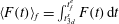 $\langle F(t)\rangle _{f}=\int _{t_{3d}^{s}}^{t_{f}^{e}}F(t)\,\text{d}t$
represents the time integral over the period of sustained turbulence (i.e.
 $t_{3d}^{s}\leqslant t\leqslant t_{f}^{o}$
).
Figure 14(d) plots the
 $\mathit{Pr}$
-dependence associated with
 $\mathscr{E}_{c}$
which avoids (by definition) the uncertainties involved in the former approach. As this figure shows, the efficiency of mixing does in fact decrease monotonically for the range of
 $\mathit{Pr}$
investigated herein. This interesting result may be construed to support the hypothesis of Mashayek & Peltier (Reference Mashayek and Peltier2013) that the route to turbulence (i.e. the detailed nature of the ‘zoo’ of secondary instabilities that populate the transition phase of flow evolution) matters insofar as mixing efficiency is concerned (Mashayek & Peltier Reference Mashayek and Peltier2013). We can argue that with an increase in
 $\mathit{Pr}$
, due to the contraction of energy-containing length scales, the turbulent eddies responsible for enhancing the background potential energy by extracting it from the APE (or equivalently the turbulent eddies that energize APE by extracting it from the kinetic energy reservoir) become less effective. Alternatively, due to an increased level of isotropy associated with the turbulent flow as
 $\mathit{Pr}$
increases, the strain field associated with turbulent eddies is weakened and thus it supports weaker scalar gradients, which in turn hinders turbulent mixing (Batchelor Reference Batchelor1959). As a consequence of this ineffectiveness associated with the energy transfer into the background potential energy, the impact of molecular
 $\mathit{Pr}$
on the irreversible mixing efficiency becomes one in which
 $\mathscr{E}_{c}$
decreases slightly at higher
 $\mathit{Pr}$
.
The moderate decrease in the mixing efficiency associated with the fully turbulent flow in our high-
 $\mathit{Pr}$
, high-
 $\mathit{Re}$
DNS analyses must be distinguished from the relatively substantial drop in
 $\mathscr{E}_{i}$
that was shown to be the case by Smyth et al. (Reference Smyth, Moum and Caldwell2001) for their low-
 $\mathit{Re}$
simulations. This new finding points once more to the importance of high
 $\mathit{Re}$
, which is the geophysically relevant regime in which the mixing efficiency remains essentially fixed to the near vicinity of the canonical value of 0.2 (as shown by the dashed lines in figure 14
d) for the initial minimum Richardson number of
 $\mathit{Ri}_{0}=0.12$
investigated here. Also, the upward concavity associated with the variations of
 $\mathscr{E}_{c}$
at higher
 $\mathit{Pr}$
suggests that mixing efficiency could asymptote to values closer to 0.1 for much higher
 $\mathit{Pr}$
, assuming that our
 $\mathit{Re}$
has reached its asymptotic value above which the mixing efficiency does not change markedly. Besides
 $\mathit{Pr}$
, the other non-dimensional number that dominantly controls the efficiency of mixing during this phase is
 $\mathit{Ri}_{0}$
, as is already evident in the analyses of Caulfield & Peltier (Reference Caulfield and Peltier2000) and most recently investigated by Mashayek et al. (Reference Mashayek, Caulfield and Peltier2013), in which they have established the existence of a non-monotonic dependence of
 $\mathscr{E}_{c}$
on
 $\mathit{Ri}_{0}$
having a maximum efficiency near
 $\mathit{Ri}_{0}=0.16$
. However, the question of whether this non-monotonicity shifts towards higher/lower
 $\mathit{Ri}$
or remains unchanged at higher
 $\mathit{Pr}$
(which is more relevant to the ocean) remains an open question.
Note that the nominal values of
 $\mathit{Re}$
and
 $\mathit{Ri}_{0}$
are simply the initial values of the investigated simulations (as listed in table 1) and do not characterize the fully developed turbulent flows generated. An alternative parameter that may be employed to characterize the stratified turbulent flows is the buoyancy Reynolds number,
 $\mathit{Re}_{b}$
as introduced in § 4.1. Figure 15 illustrates the time variations of
 $\mathit{Re}_{b}$
for all of the values of
 $\mathit{Pr}$
that have been investigated, showing that they all reach values as high as
 $\mathit{Re}_{b}\approx 150{-}250$
at the onset of fully developed flow, as pointed out earlier in § 4.1. Insofar as the impact of
 $\mathit{Pr}$
on the mixing efficiency is concerned, in this paper we have developed a physical understanding as to why mixing efficiency decreases at higher
 $\mathit{Pr}$
. Ascribing such behaviour to
 $\mathit{Re}_{b}$
or
 $\mathit{Re}_{{\it\lambda}}$
(see the appendix A for a discussion of
 $\mathit{Re}_{{\it\lambda}}$
) or other variations of parameters would simply be to rephrase the question as to why these additional parameters change in the way they do with
 $\mathit{Pr}$
. Furthermore, since mixing efficiency varies non-monotonically with
 $\mathit{Re}_{b}$
, it is not a trivial matter as to how one might simply characterize the decrease in mixing efficiency with
 $\mathit{Re}_{b}$
.
Time variations of the buoyancy Reynolds number
 $\mathit{Re}_{b}=$
 $|\mathscr{D}|/({\it\nu}\langle N^{2}\rangle _{z})$
for all of the three-dimensional DNS analyses with different values of
 $\mathit{Pr}$
.

(a) The time series associated with background potential energy
 $\mathscr{P}_{B}$
for various
 $\mathit{Pr}$
, demonstrating a decrease in entrainment of ambient flow (reduced rise in
 $\mathscr{P}_{B}$
). (b) Vertical profile of density
 $\overline{{\it\rho}}=\langle {\it\rho}\rangle _{xy}$
showing a reduction in stratified shear layer expansion with increasing
 $\mathit{Pr}$
after the flow is re-laminarized.

6.2. The effect of
 $\mathit{Pr}$
on entrainment

Figure 16(a) illustrates the time variation of the background potential energy,
 $\mathscr{P}_{B}$
, a notional state of static stability which has been obtained after an adiabatic rearrangement of the density field into a monotonically decreasing upward assembly following the method depicted in figure 1. The total rise in
 $\mathscr{P}_{B}$
is directly linked to the total entrainment of the ambient flow on the flanks of the shear layer into the central mixing region. As figure 16(a) demonstrates, such a rise is suppressed as
 $\mathit{Pr}$
increases, which is in accord with what we had predicted on the basis of our observation from figure 7 regarding the total loss in kinetic energy of the flow. Another indication of the occurrence of less effective entrainment at higher
 $\mathit{Pr}$
can be seen on the basis of the ultimate stratified shear layer thickness after the flow is re-laminarized. Figure 16(b) illustrates the density profiles associated with the re-laminarized shear layer for the range of
 $\mathit{Pr}$
we have investigated. This plot shows that the eventual expansion of the stratified shear layer is reduced following the end of the turbulent life cycle in fluids with higher molecular Prandtl number, which also suggests that at higher
 $\mathit{Pr}$
, the processes involved during the course of turbulence evolution would become less effective insofar as entrainment is concerned.
Here it might be puzzling why different rates of density and momentum diffusion would physically lead to such variation in the re-laminarized shear layer thickness, or the total gain in the background potential energy, given the impact of
 $\mathit{Pr}$
on promoting the strength of the eyelid instability (see § 3), as the primary catalyst for driving the irreversible mixing process. A plausible argument resolving this conundrum can be stated in two equivalent ways. (I) Increasing
 $\mathit{Pr}$
not only strengthens the major secondary instabilities but also reduces the associated energy-containing length scales (for example, see the reduced horizontal scale of the shear-aligned convective rolls in figure 8), which overall reduces their effectiveness in entraining fast moving fluid on the flanks of the shear layer into the well-mixed region near the original inflection point of the shear profile. Alternatively (II), due to the presence of the ultraviolet catastrophe at higher
 $\mathit{Pr}$
(actually plausible only in the limit of extremely high
 $\mathit{Pr}$
), kinetic energy of the flow is directly injected into the dissipation subrange (i.e. the Batchelor scale) and hence a quasi-steady turbulent phase occurs. However, at low
 $\mathit{Pr}$
, interactions between filaments of considerably larger length scales are precursors to the full downscale cascade of energy. As a consequence, shear layers with lower
 $\mathit{Pr}$
contain significantly larger coherent structures than their higher-
 $\mathit{Pr}$
counterparts during the same phase and the entrainment of fast-moving fluid from the flanks of the shear layer becomes more efficient, thereby leading to the increase of the background potential energy and the associated entrainment.
7. Summary and conclusions
The turbulence that is engendered by breaking of a nonlinear Kelvin–Helmholtz wave serves as a useful context for the study of diapycnal mixing in stratified shear flows, and is perhaps especially appropriate for abyssal ocean applications. This mechanism also occurs ubiquitously in both the oceans and the atmosphere (Thorpe Reference Thorpe2005), where it facilitates an upward vertical diffusivity of fluid mass. For the oceans in particular, this mechanism is assumed to play a vital role in determining the effective diapycnal diffusivity that enables upwelling of abyssal waters back to the surface of the southern ocean so as to close the deep component of the MOC. Since the density stratification in the oceans is controlled by both temperature and salinity, and due to the differences in their molecular diffusivities
 ${\it\kappa}_{s}\approx 10^{-2}{\it\kappa}_{T}$
, the molecular Prandtl number is much higher than unity and might be expected to vary in the range
 $\mathit{Pr}=O(7{-}700)$
.
Motivated by the expected characteristics of this realistic oceanographic regime, in this paper we have investigated a numerically challenging portion of the three-dimensional parameter space determined by the non-dimensional parameters
 $\mathit{Re}$
,
 $\mathit{Pr}$
and
 $\mathit{Ri}$
. Our focus was upon the impact of increasing Prandtl number as high as
 $\mathit{Pr}=16$
at a fixed high Reynolds number of
 $\mathit{Re}=6000$
and a fixed value of initial minimum Richardson number
 $\mathit{Ri}_{0}=0.12$
, for which inviscid instability is expected by the Miles–Howard theorem. For the purpose of the DNS analyses upon which our investigation was based, we employed a high-order spectral element code, Nek5000, which has proved to be ideally suited for this work on account of its computational accuracy as well as its massively parallel scalability. Furthermore, a parallel implementation (see figure 1) was successfully implemented for the global sorting of the density profiles, which is required for calculation of the irreversible mixing and therefore mixing efficiency.
The nature of secondary instabilities that mediate the transition to turbulence and grow upon the evolving structure of the primary Kelvin–Helmholtz instability were found to change substantially with increase in the molecular Prandtl number. We explored the changing nature of these secondary instabilities using a variety of methods, including (I) non-separable linear stability analysis, (II) detailed visualizations of the flow field, and (III) spectral decompositions of flow in the spatial locations within the parent KH wave where modes of various type were expected to originate. The significant findings in this regard may be summarized as follows.
(i) The ‘braid instability’ was the FGM in all our linear analyses of secondary instabilities and included both the SPI (which develops at the centre of the braid) and the secondary shear instability on the braid as branches of the same family of instabilities (although different in their dimensionality), competing against each other depending on the relative strength of the braid shear and strain fields. For our choice of
 $\mathit{Re}$
and
 $\mathit{Ri}_{0}$
it was shown that the SPI emerged as the prominent branch while the secondary shear instability only appeared after other instabilities had emerged. It was also illustrated that an increase in
 $\mathit{Pr}$
suppresses the SPI due to possible indirect weakening of the braid strain field, caused by the convectively driven component of the eyelid instability.
(ii) The ‘eyelid instability’ was the second FGM in all our analysed cases. This mode was characterized as a mixed convection/shear-driven instability, a high-
 $\mathit{Re}$
manifestation of the conventional secondary shear-aligned convective instability. The newly discovered shear-driven characteristic of this mode was shown to be realized as counter-rotating spanwise vortices that grow around the eyelid and move along the shear, populating the diagonal corners of the billow. Both characteristics of the eyelid instability are strongly coupled and are promoted as
 $\mathit{Pr}$
increases. Furthermore, for higher
 $\mathit{Pr}$
, the wavenumber associated with the maximum growth rate shifts towards shorter wavelengths, as revealed by the increased number of convective rolls (in the spanwise direction) and counter-rotating vortices (in the streamwise direction). Such length scale contraction was established to be a principal effect of increasing
 $\mathit{Pr}$
.
(iii) In addition, while both the stagnation point ‘braid’ instability and the ‘eyelid’ instability were shown to be highly three-dimensional, only the latter is capable of promoting short-wave instabilities at high values of
 $\mathit{Pr}$
and hence flattening the growth rate versus spanwise wavenumber curve (see figures 3
a and 6).
(iv) The pairing instability, which acts to amalgamate adjacent vortex cores and hence supports an inverse cascade of energy to horizontal length scales above the injection scale, was found to remain suppressed at Prandtl numbers higher than unity, implying high
 $\mathit{Re}$
to be the fundamental requirement for its suppression, as previously established by Mashayek & Peltier (Reference Mashayek and Peltier2012a
, Reference Mashayek and Peltier2013). This finding further strengthens the explanation of observations regarding the effective absence of this mechanism in nature.
(v) No instability was found central to the billow core, and it was demonstrated in our flow visualizations and spectral decomposition that a ‘quiet’ core (as observed by Geyer et al.
Reference Geyer, Lavery, Scully and Trowbridge2010) is a direct consequence of high-
 $\mathit{Re}$
flow, and should not be interpreted as an indication of the occurrence of early homogenization of the core by secondary instabilities focused in this region.
It is important to emphasize that, for geophysical flows with very high Reynolds numbers, it is usually assumed that shear-induced turbulence is
 $\mathit{Pr}$
-independent by invoking Reynolds number similarity (see e.g. Lozovatsky & Fernando Reference Lozovatsky and Fernando2012). However, as we have shown in this paper, the ‘eyelid instability’ plays a paramount role in the transition process, one which is also potentially capable of injecting turbulence directly into all scales of motion in the limit of much higher
 $\mathit{Pr}$
, characteristic of salt-stratified parts of the ocean. In particular, the Rayleigh number associated with the convection engendered by this mode is inevitably influenced by
 $\mathit{Pr}$
whose impact on three-dimensionality of the turbulence is far from being negligible. Therefore we believe this issue requires further investigation in the future.
The most striking influence of increasing molecular Prandtl number on the secondary instabilities must be attributed to its role in length scale contraction that we have interpreted as suggestive of an ‘ultraviolet catastrophe’ in the limit of much higher
 $\mathit{Pr}$
. More precisely, we have shown that even at the time of saturation of the two-dimensional KH wave, as
 $\mathit{Pr}$
increases there is a strong tendency for the spectral power of the eyelid instability to grow rapidly at a wider range of higher spanwise wavenumbers rather than simply at the scale of an FGM, such that the spectral gap between short-wave and long-wave instabilities diminishes gradually. This influence of the Prandtl number could plausibly explain the observations of Geyer et al. (Reference Geyer, Lavery, Scully and Trowbridge2010) by noting the difference in the structure of KH billows detected in the atmosphere (where waves most often appear to be almost laminar) as opposed to the ocean (where they appear to be inevitably turbulent). More precisely, the abundance of the small-scale coherent structures at the periphery of the billow and on its braid does not imply a ‘shear-dominated’ or braid-induced mixing (as inferred by Geyer et al.
Reference Geyer, Lavery, Scully and Trowbridge2010), but is probably an inevitable manifestation of the short-wave instabilities attributed to a mixed convection/shear-driven mode, and thus the occurrence of the ultraviolet catastrophe that characterizes transition in the high-
 $\mathit{Re}$
, high-
 $\mathit{Pr}$
regime.
It is important to be clear that the relevant scales of motion that are affected (directly or indirectly) by the impact of
 $\mathit{Pr}$
on the secondary instabilities do not reach anywhere near the dissipation scale for the range of
 $\mathit{Pr}$
investigated in this paper (
 $1\leqslant \mathit{Pr}\leqslant 16$
). In fact the Kolmogorov and Batchelor scales would be entirely off the scale if they were included in figures 12 and 13, for example. That being said, based on the trends of the growth rate with increasing
 $\mathit{Pr}$
(see e.g. figures 6 and 12), we have conjectured to the effect that an ultraviolet catastrophe might be realized in the limit of very high Prandtl numbers whereby the dissipation scales would be energized directly. It is very interesting to note that in the context of DNS studies of isotropic turbulent mixing of a passive scalar (i.e. non-stratified), based on moderate to very high Prandtl (or Schmidt) numbers (e.g. Yeung, Donzis & Sreenivasan Reference Yeung, Donzis and Sreenivasan2005; Donzis, Sreenivasan & Yeung Reference Donzis, Sreenivasan and Yeung2010), it is suggested that the spectrum rolls off in the so-called viscous-convective range where it follows a
 $-1$
power law (Batchelor Reference Batchelor1959) as opposed to a
 $-5/3$
power law, where the latter is characteristic of such turbulent flows at sufficiently high Reynolds numbers but at
 $\mathit{Pr}=O(1)$
(see Gotoh & Yeung Reference Gotoh, Yeung, Kaneda, Davidson and Sreenivasan2013 for a review). This is somewhat reminiscent of what we refer to in this paper as the emergence of shorter-wavelength instabilities as
 $\mathit{Pr}$
increases. This important issue, however, warrants a careful separate investigation in order to study possible changes in the spectral cascade behaviour of shear-induced stratified turbulence at higher values of
 $\mathit{Pr}$
.
Insofar as the turbulent phase of the flow evolution is concerned, interesting consequences have been demonstrated in this paper due to the important changes in the nature of the energy budget of the breaking KH wave that occurs as the Prandtl number increases. At high molecular Prandtl number, the turbulent kinetic energy achieves its saturation level more rapidly because the route to turbulence, which involves a nonlinear process of successive instabilities transferring the energy towards smaller scales, is shortened. In other words, for higher
 $\mathit{Pr}$
, an equable distribution of energy across a wider range of wavenumbers facilitates the process of downscale energy cascade. Moreover, and for the same reason, the original anisotropy of the stratified shear flow associated with the two-dimensional structure of the primary KH wave is less evident on the smaller scales as
 $\mathit{Pr}$
increases, because the turbulent flow becomes more disorganized when a broader range of scales of motion are simultaneously energized, which serves to minimize flow anisotropy at high
 $\mathit{Pr}$
.
The efficiency of mixing associated with the extent of the irreversible rise of background potential energy, as compared to the total dissipated energy, also varies with the molecular Prandtl number during all phases of flow evolution. In particular, during the fully developed turbulent phase, as
 $\mathit{Pr}$
increases there is a modest monotonic decrease in the cumulative mixing efficiency, which might be attributed to the changes in the nature of secondary instabilities that are caused by increasing
 $\mathit{Pr}$
. One possible mechanism that might be adversely affected by an increase in
 $\mathit{Pr}$
is that the energized length scales would contract, thereby becoming less effective in extracting energy from the accessible energy reservoirs. Alternatively we might attribute the reduced effectiveness of mixing at high
 $\mathit{Pr}$
to the increasing isotropy of the turbulence as
 $\mathit{Pr}$
increases and a reduced strain deformation field. We have conjectured that the monotonic decrease of mixing efficiency with increasing Prandtl number might eventually asymptote to a constant, but this must remain a speculation that will require further work to properly establish.
We have also noted that the entrainment of fluid from the flanks of the shear layer into the turbulent mixing region is manifested in the total rise in the background potential energy, which in turn is related to the net drop in the total kinetic energy of the flow. We found that as
 $\mathit{Pr}$
increases, the entrainment decreases and the ultimate expansion of the re-laminarized stratified shear layer also decreases. Such changes in entrainment are related to the same length scale contraction, which renders shear-aligned convective rolls individually more compact in the horizontal spanwise direction. However, since convective cells in general are commonly recognized as having an aspect ratio near unity, such horizontal contraction in length scale translates directly into an equivalent contraction in the vertical length scales, and hence the fluid filaments are less effective at extracting kinetic energy from the background flow outside of the shear layer. As a result, the rise in the background potential energy and therefore the associated entrainment is inhibited as the molecular Prandtl number increases.
There are many outstanding questions that still remain to be addressed in future work. For example, and most importantly, it would be of particular interest to directly address the implications of our detailed analyses for the parametrization of small-scale diapycnal diffusivity processes in large-scale models of the ocean’s general circulation. In this regard, it will also be important to firmly establish a robust connection between the molecular and turbulent values of the Prandtl number.
Acknowledgements
H.S. would like to extend his thanks to Dr P. Fischer for his kind and helpful guidance in the use of Nek5000 for both DNS simulations and for post-processing purposes. We are also grateful to B. Smyth, C. Caulfield, R. Geyer and three anonymous reviewers whose constructive comments have further improved the paper. Computations were performed on the BG/Q supercomputer at the SciNet HPC Consortium of the University of Toronto. SciNet is funded by the Canada Foundation for Innovation under the auspices of Compute Canada; the Government of Ontario; Ontario Research Fund – Research Excellence; and the University of Toronto. The research of W.R.P. at the University of Toronto is sponsored by NSERC Discovery Grant A9627.
Supplementary data
Supplementary data are available at http://dx.doi.org/10.1017/jfm.2015.225.
Appendix A
Fully turbulent flows are usually characterized by having invariant flow properties at Reynolds numbers higher than a transitional value. As discussed in § 2.2, our nominal value of initial Reynolds number (
 $\mathit{Re}=6000$
, see table 1) has been shown to be high enough to ensure that mixing efficiency remains relatively constant for simulations with initial Reynolds numbers as high as
 $\mathit{Re}=10\,000$
(see Mashayek & Peltier Reference Mashayek and Peltier2013, their figure 22). Nonetheless, another measure on the basis of which we may assess the extent to which the flow has become fully turbulent involves the Taylor microscale Reynolds number
 $\mathit{Re}_{{\it\lambda}}$
. In the context of shear-induced stratified turbulence, a careful investigation of a specific value for
 $\mathit{Re}_{{\it\lambda}}$
, which enables a clear distinction to be made between transitional and fully turbulent flows, is unavailable and we believe this issue to remain non-trivial for stratified turbulent flows. Nonetheless, some studies of homogeneous passive scalar mixing suggest the transitional value of
 $\mathit{Re}\approx 10\,000$
or
 $\mathit{Re}_{{\it\lambda}}=100$
, where
 $\mathit{Re}_{{\it\lambda}}\approx \sqrt{Re}$
(see e.g. Dimotakis Reference Dimotakis2005). Our intention in this appendix is to evaluate the relevant values of
 $\mathit{Re}_{{\it\lambda}}$
associated with the simulations discussed in the paper.
Figure 17 illustrates the variations of
 $\mathit{Re}_{{\it\lambda}}$
for all the flows investigated in this paper, in which
 $\mathit{Re}_{{\it\lambda}}$
is calculated based on the following expressions (Smyth & Moum Reference Smyth and Moum2000b
):
 $$\begin{eqnarray}\mathit{Re}_{{\it\lambda}}=\frac{q{\it\lambda}}{{\it\nu}},\quad {\it\lambda}=\left(\frac{5{\it\nu}q^{2}}{|\mathscr{D}|}\right)^{1/2}.\end{eqnarray}$$
Note that in figure 17(a),
 $q=\sqrt{2(\mathscr{K}_{2d}+\mathscr{ K}_{3d})}$
has been assumed, whereas in figure 17(b),
 $q=\sqrt{2\mathscr{K}_{3d}}$
is assumed.
The Taylor microscale Reynolds number in figure 17(a) reaches values as high as
 $O(10^{3})$
at the saturation point of the two-dimensional KH wave and is of
 $O(10^{2})$
at the onset of what we refer to as the fully turbulent regime (see § 4.1 for the definition of these times and for our definition of the fully turbulent regime). The maximum value of
 $\mathit{Re}_{{\it\lambda}}=O(10^{3})$
at
 $t_{2d}^{s}$
occurs in the absence of turbulence, which is therefore misleading. Alternatively,
 $\mathit{Re}_{{\it\lambda}}$
in figure 17(b) reaches a maximum of
 $O(10^{2})$
(in the range 50–80). However, the problem is that
 $\mathscr{K}_{3d}$
only captures the ‘three-dimensional’ fluctuations of the fully turbulent flow. In other words, it does not necessarily capture the spanwise averaged small-scale turbulence. Therefore, the values of
 $\mathit{Re}_{{\it\lambda}}$
at the onset of turbulence (in the range
 $t=130{-}150$
) in figure 17(a) produce a more relevant estimate for the value of
 $\mathit{Re}_{{\it\lambda}}$
and thus
 $\mathit{Re}_{{\it\lambda}}=O(10^{2})$
is high enough (for all
 $\mathit{Pr}$
studied here) to be associated with the fully turbulent regime.
Time variations of the Taylor microscale Reynolds number (A 1) calculated based on (a) the two- and three-dimensional components of the kinetic energy
 $q=\sqrt{2(\mathscr{K}_{2d}+\mathscr{ K}_{3d})}$
, and (b) only the inherently three-dimensional component of the kinetic energy
 $q=\sqrt{2\mathscr{K}_{3d}}$
.