
1. Introduction
The formation process of a vortex ring has been of interest in the field of vortex dynamics since the early works by Maxworthy (Reference Maxworthy1972) and Didden (Reference Didden1979). With a piston–cylinder configuration ejecting a finite volume of fluid, the relationships between parameters such as stroke length and stroke velocity profile and the resulting vortex ring dynamics were investigated, and a universal time scale characterizing the vortex ring formation process was introduced (Gharib, Rambod & Shariff Reference Gharib, Rambod and Shariff1998; Mohseni & Gharib Reference Mohseni and Gharib1998). It was later revealed that the formation process differs depending on the velocity profile of the discharge piston (Rosenfeld, Rambod & Gharib Reference Rosenfeld, Rambod and Gharib1998), the compressibility of the fluid (Arakeri et al. Reference Arakeri, Das, Krothapalli and Lourenco2004; Dora et al. Reference Dora, Saravanan, Karunakar and Das2011) and the shape of the nozzle exit (Gao et al. Reference Gao, Yu, Ai and Law2008). Gao & Yu (Reference Gao and Yu2010) introduced a two-stage analytic model of the development of a vortex ring for different nozzle exits to describe the physical process of pinch-off, which closely matched the experimental results of Gharib et al. (Reference Gharib, Rambod and Shariff1998) and Gao et al. (Reference Gao, Yu, Ai and Law2008). The accuracy and limitation of the analytic model were evaluated in detail using experimental data for a clean vortex ring (Das, Bansal & Manghnani Reference Das, Bansal and Manghnani2017). The principles of vortex ring formation have been used to better understand the underlying mechanisms of biological and bio-inspired systems for propulsion and fluid transport (Dabiri Reference Dabiri2005; Dabiri & Gharib Reference Dabiri and Gharib2005a,Reference Dabiri and Gharibb; Gharib et al. Reference Gharib, Rambod, Kheradvar, Sahn and Dabiri2006; Dabiri et al. Reference Dabiri, Colin, Katija and Costello2010).
In addition to the vortex ring formation process itself, the entrainment of the surrounding fluid by a developing vortex ring has been studied. Based on the pioneering study by Maxworthy (Reference Maxworthy1972), in which the vorticity diffusion of an isolated vortex ring was coupled with fluid entrainment using dye and hydrogen-bubble visualization, more recent investigations have explored the fluid entrainment of a vortex ring by analysing the evolution of instantaneous velocity fields. Dabiri & Gharib (Reference Dabiri and Gharib2004) computed the entrainment fraction by measuring experimentally the volume of an isolated vortex ring from velocity fields. Furthermore, time-varying fluid entrainment and detrainment were examined from the perspective of Lagrangian coherent structure both numerically (Shadden et al. Reference Shadden, Katija, Rosenfeld, Marsden and Dabiri2007) and experimentally (Shadden, Dabiri & Marsden Reference Shadden, Dabiri and Marsden2006; Olcay & Krueger Reference Olcay and Krueger2008).
Besides studies of a single vortex ring, there have also been numerous studies about the mutual interaction of vortex rings placed on a co-axis (e.g. Oshima, Noguchi & Oshima Reference Oshima, Noguchi and Oshima1986; Riley & Stevens Reference Riley and Stevens1993). In particular, the leapfrogging behaviour of co-rotating vortex rings was studied both numerically and experimentally in order to find the circumstances under which the leapfrogging phenomenon can occur over several cycles for a pair of vortex rings (Lim Reference Lim1997; Satti & Peng Reference Satti and Peng2013) and multiple vortex rings (Cheng, Lou & Lim Reference Cheng, Lou and Lim2015; Qin, Liu & Xiang Reference Qin, Liu and Xiang2018). They also provided some insight into the merger process of vortex rings.
Although many studies have been carried out to understand diverse aspects of vortex ring formation and their mutual interaction, the coupling of a vortex ring ejected from a cylinder with a bluff body propagating ahead of the vortex ring remains unexplored. The translation of a bluff body in a fluid medium develops a wake structure behind the body, which undergoes roll-up and pinch-off processes similar to those of a piston-generated vortex ring (Fernando & Rival Reference Fernando and Rival2016; Fernando et al. Reference Fernando, Marzanek, Bond and Rival2017). Hence, in the configuration of a vortex ring with a forward-moving bluff body in front of it, the vortex ring formation may be strongly affected by the wake produced from the bluff body. A model similar to this configuration can be found in the launch mechanism of Sphagnum spores (Sundberg Reference Sundberg2005, Reference Sundberg2010; Whitaker & Edwards Reference Whitaker and Edwards2010), which was in fact the motivation for the present study. During the dehiscence of a spore capsule, the internal compression of the capsule is induced by its deformation from a spherical shape to a cylindrical one, and as a result the cap of the capsule can pop up. When the cap opens, the compressed air is ejected from the capsule, forming a vortex ring. Whitaker & Edwards (Reference Whitaker and Edwards2010) claimed that the spores captured inside the vortex ring could propagate a greater distance compared with a single spore particle of the same initial velocity in static ambient air. Although the advantage of the formed vortex ring on transporting individual spores was suggested, the fluid-mechanical interaction between the detached cap and the jet from the capsule and its influence on the development of a vortex ring still remains unclear; this is also important to better understand the shooting mechanism of the spore capsules. Because the sources of the two vortex structures, i.e. the starting jet from the capsule and the wake of the forward-moving cap, are initially at the same position, it is clear that these two vortices will interact throughout the launch process.
Here, we examine experimentally the formation and fluid transport of a vortex ring that couples with the wake structure generated by a translating hemispherical cap. This study aims at obtaining a useful insight into the fluid transport and entrainment of a vortex ring subject to an actively moving bluff body. Furthermore, it will help us to better understand the biological implications of spore discharge dynamics. The experimental set-up is described in § 2. The characteristics of vortex interaction and fluid entrainment observed and their dependence on kinematic parameters, such as stroke length and the velocities of the cap and piston, are discussed in §§ 3.1 and 3.2, respectively. The circulation of the coupled vortex structures is analysed in § 3.3, which is followed by simple analytical modelling for the transition of vortex modes in § 3.4 and concluding remarks in § 4.
2. Experimental set-up
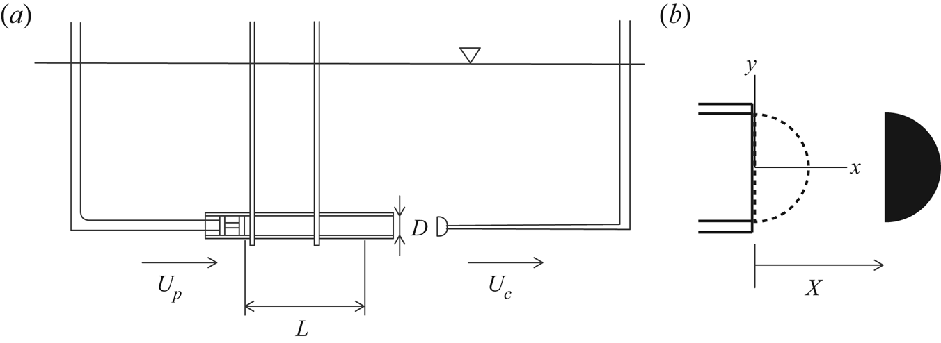
Experiments were conducted in a water tank of width 490 mm, length 1200 mm and height 500 mm (figure 1). A piston–cylinder apparatus was constructed to produce a vortex ring. The cylinder, of internal diameter  $D=20$ mm, was made of acrylic, and the piston was fabricated by a 3D printer (Ultimaker
 $2+$, Ultimaker Inc.) from polylactic acid. The fabricated piston was tested to ensure that there was no leakage between the cylinder and the piston. As a bluff body, a fully filled hemispherical cap was printed using the same 3D printer and material, and it was initially placed in contact with the open end of the cylinder from which water was ejected by the action of the piston. For translation, the piston and the hemispherical cap were each connected to a linear guide (MW-EQB45, NTRexLAB) mounted above the water tank. The stepper motors for the two linear guides were controlled by a computer via a data acquisition board (PCIe-6321, National Instrument Co.). The kinematics of the piston and the cap were prescribed with MATLAB (Mathworks Inc.): both started impulsively from rest and translated with constant velocity.
(a) Schematic diagram of the experimental set-up. (b) The initial position of the cap is shown by the dashed line. The distance between the right end of the cylinder and the back surface of the translating cap is denoted by  $X$.

The ratio of stroke length  $L$ to cylinder diameter
 $D$ is the main parameter determining the formation of a vortex ring in the piston–cylinder apparatus (Gharib et al. Reference Gharib, Rambod and Shariff1998). This stroke ratio
 $L/D$ is therefore taken as one of the variables in our study, with value varying from 2 to 4; at
 $L/D = 4$, a fully developed vortex ring pinches off from the exit of the cylinder, and no trailing jet is formed behind the vortex ring (Gharib et al. Reference Gharib, Rambod and Shariff1998). To characterize the interaction between the starting jet ejected by the cylinder and the wake shedding from the cap, we also consider the ratio of the translational speeds of the cap (
 $U_{c}$) and the piston (
 $U_{p}$):
 $U_{c}/U_{p} = 0.17\text {--}3.0$. To ensure that the Reynolds number of our experiment is of the same order of magnitude as that of an actual Sphagnum spore jet computed using the viscosity of air, the initial launch velocity and diameter of the spore capsule (Whitaker & Edwards Reference Whitaker and Edwards2010), the velocities of the piston and the cap vary between 2.5 and
 $15.0\ \textrm {cm}\,\textrm {s}^{-1}$. Accordingly, the Reynolds number based on the cap velocity,
 $Re_{c}\ (=U_{c}D/\nu )$, ranges from 500 to 3000, and the Reynolds number based on the piston velocity,
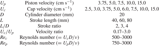
 $Re_{p}\ (=U_{p}D/\nu )$, is between 750 and 3000. The values of the experimental parameters are listed in table 1.
Experimental parameters.

Particle image velocimetry (PIV) was conducted to obtain velocity fields. Images were captured at 500 frames per second by a high-speed camera (MINI-UX50, Photron Inc.) with a resolution of  $1280 \times 1024$ pixels. Hollow glass particles with an average density of
 $1.6\ \textrm {g}\,\textrm {ml}^{-1}$ and a mean diameter of
 $14\ \mathrm {\mu }\textrm {m}$ (SH400S20, Potters Industries) were seeded inside the tank; this particle size was large enough for illumination while minimizing subpixel particles. A 10 W continuous laser (MGL-W-532A, CNI Co.) was used to make a planar laser sheet on the
 $(x,z)$ plane (figure 1b). Cross-correlation of the image pairs was performed with a multiple-pass interrogation method (PIVview2C 3.6, PIVTEC GmbH). A window size of
 $24 \times 24$ pixels with 50 % overlap was chosen for the experimental cases with a cap, yielding
 $105 \times 84$ nodes and a spatial resolution of 1.5 mm. The time interval between a pair of images was adjusted to be 4 ms for the cases with
 $U_{c} = 2.5\text {--}7.5\ \textrm {cm}\,\textrm {s}^{-1}$ and 2 ms for
 $U_{c} = 10$ and
 $15\ \textrm {cm}\,\textrm {s}^{-1}$. For the cases without a cap (i.e. those with only a single vortex ring), a window size of
 $32 \times 32$ pixels and a time interval of 4 ms were chosen instead; the spatial resolution was approximately 2.2 mm. The vorticity field was obtained from the velocity field with a central difference scheme.
For PIV experiments, the size and seeding density of particles were adjusted so that approximately 10 particles were present in a single interrogation window, with individual particles having three to four pixels in size on average. The maximum displacement of particles between the two images of a pair was carefully adjusted to be within one-sixth of the length of the window (Willert & Gharib Reference Willert and Gharib1991). To ensure the accuracy of the PIV results, the divergence of the velocity field was first evaluated. Although the divergence should be zero in the ideal case of incompressible flow, the magnitude of the divergence evaluated over the entire fluid domain was within  $O(10^{-4}\ \textrm {s}^{-1}$). This is very small compared with the maximum vorticity observed in our cases, which is four to five orders of magnitude higher, suggesting that our data are reliable. Furthermore, although a direct comparison was not appropriate due to minor differences in the dimensions of the experimental apparatus used, the circulations of the fully developed vortex ring for the no-cap cases of
 $L/D = 4$ and
 $Re_{p} = 1500$ and 3000 (corresponding to
 $U_{p} = 7.5$ and
 $15.0\ \textrm {cm}\,\textrm {s}^{-1}$) are
 $\varGamma \approx 28$ and
 $55\ \textrm {cm}^{2}\,\textrm {s}^{-1}$ averaged over time, respectively, and these values are in good agreement with the experimental results of Gharib et al. (Reference Gharib, Rambod and Shariff1998); the differences are within 10 %. For the definition of the circulation in our experiments, see the first paragraph of § 3.3.
In addition, the circulation values of our experiment match the slug model with good accuracy (Green Reference Green1995). The circulations for the  $L/D = 2$ cases without a cap showed only 5 % difference from the value calculated by the model of Sullivan et al. (Reference Sullivan, Niemela, Hershberger, Bolster and Donnelly2008) that is known to be accurate for small stroke length. The circulations of the
 $L/D = 4$ cases without a cap were also compared with the value by the model of Shusser et al. (Reference Shusser, Rosenfeld, Dabiri and Gharib2006). Dimensionless circulations of our cases were approximately 1.24, which is very close to the value of 1.26 by Shusser et al. (Reference Shusser, Rosenfeld, Dabiri and Gharib2006). To confirm the repeatability of the PIV results, the experiments were repeated five times for the case of
 $L/D = 3$ and
 $Re_{p} = 1000$ (
 $U_{p} = 10\ \textrm {cm}\,\textrm {s}^{-1}$) without a cap. The maximum difference of the circulation from its mean value was 5 % throughout the entire propagation time, which demonstrates that our experiments were repeatable.
In addition, laser-induced fluorescence (LIF) was used with fluorescein dye to visualize how the fluid volume initially inside the cylinder is ejected and follows the forward-moving cap. A quantity (40 ml) of dye premixed in water with a constant concentration of  $0.4\ \textrm {g}\,\textrm {L}^{-1}$ was injected into the chamber inside the cylinder using a syringe, and the premixed dye replaced the entire volume of the chamber. Owing to the illumination of the dye by the laser sheet, the water–dye mixture initially inside the cylinder and the ambient water initially outside the cylinder could be distinguished easily. After each experiment, the dye was refilled in order to ensure a uniform dye concentration and to reduce uncertainties in tracking the dyed fluid during image processing. LIF images were captured at 500 frames per second with the same high-speed camera as used for PIV (MINI-UX50, Photron Inc.), and the spatial resolution of the LIF images was approximately 0.14 mm per pixel. The dye was illuminated by the same continuous laser (MGL-W-532A, CNI Co.). The transport of the dyed fluid was quantified after image processing using MATLAB. A detailed procedure for quantitative analysis will be presented in § 3.2.
Experiments using two different dye colours were also carried out to visualize the interaction of the two vortex structures generated by the piston and the cap. Green fluorescein dye initially injected inside the cylinder visualized the starting piston jet from the apparatus, while red rhodamine B dye ejected on the surface of the cap visualized the wake produced by the translating cap. As the cap translated, the rhodamine dye with an initial concentration of  $0.5\ \textrm {g}\,\textrm {L}^{-1}$ was ejected simultaneously on the surface of the cap through a thin stainless-steel pipe with an outer diameter of 1 mm. The stainless-steel pipe was attached to the acrylic structure connecting the cap to the linear guide. The volume flow rate of the rhodamine dye and water mixture was controlled from 1.5 to
 $9\ \textrm {ml}\,\min ^{-1}$ using a syringe pump (SP-8800, AMPall Co.). The volume flow rate depended on the translational speed of the cap,
 $U_{c}$. Images were filmed with a high-speed colour camera (FASTCAM SA-Z, Photron Inc.) at 1000 frames per second, and a 500 W halogen lamp (KE-2WL, Korea Electric) was used as light source.
3. Results and discussion
3.1. Vortex modes
In our model, three distinct modes are observed for the mutual interaction of vortex structures: an attached mode, a spill mode and a detached mode. From PIV, it is difficult to distinguish the flow structure generated from the piston and the flow structure generated from the cap because the vorticities of these two flow structures have the same sign on the same side. Accordingly, vorticity and velocity fields from PIV are not ideal for classifying the vortex modes and visualizing the coupling of the two flow structures. Therefore, we used two-dye visualization to examine the vortex modes, although this has a limitation in quantitative analysis. The correlation between the vortex modes and the circulation/vorticity distribution obtained from PIV will be discussed in § 3.3.
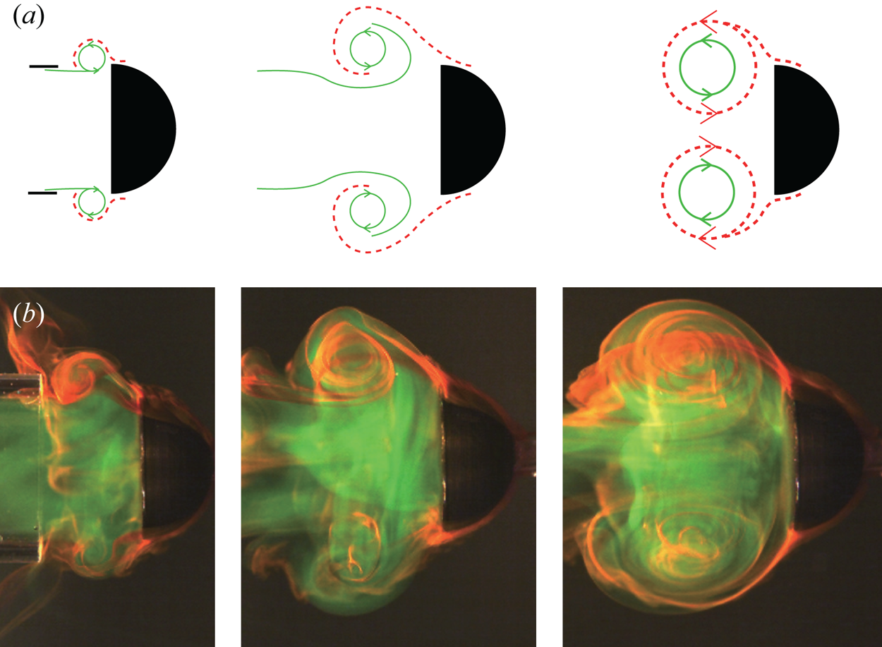
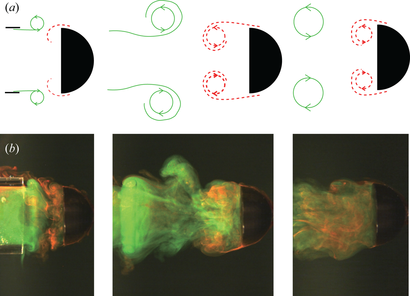
The attached mode, which is our main interest in this study, arises in the intermediate range of the velocity ratio  $U_{c}/U_{p}$ between the spill mode and the detached mode (figure 2). During the initial formation phase, roll-up of the starting jet from the cylinder (green solid line in figure 2a) captures the wake structure generated at the edge of the cap (red dashed line in figure 2a). These two separate vortices merge together and evolve into a single vortex structure (
 $U_{p}t/L = 1.88$ in figure 2). The merged vortex structure remains attached to the cap and translates together with the cap.
(a) Schematic diagram of the formation of the attached mode. The green solid line is the starting jet from the cylinder, and the red dashed line is the wake from the cap. (b) Corresponding images from the two-dye experiment at three instants:  $U_{p}t/L = [0.33, 0.89, 1.88]$. Here
 $L/D = 4$,
 $U_{c}/U_{p} = 0.5$ and
 $Re_{p} = 3000$ (
 $U_{p} = 15.0\ \textrm {cm}\,\textrm {s}^{-1}$). See the supplementary movie available at https://doi.org/10.1017/jfm.2020.633 for (b).

The overall shape and size of the combined vortex structure are similar to those of a single vortex ring in the absence of the cap. However, in the attached mode, the propagation speed of the fully developed vortex structure becomes almost identical to the translational speed of the cap, indicating that the propagation of vortex structure is controlled by the forward-moving body. The propagation speed of a single vortex ring with no cap is given by
 \begin{equation} U_{tr} = \frac{\varGamma}{4{\rm \pi} R}\left[\ln\frac{8}{\epsilon}-\frac{1}{4}+ \frac{3\epsilon^2}{8}\left(\frac{5}{4}-\ln\frac{8}{\epsilon}\right)\right], \end{equation}
where  $\epsilon$ =
 $a/R$,
 $a$ is the radius of the vortex core and
 $R$ is the radius of the vortex ring, which is the second-order formula derived by Fraenkel (Reference Fraenkel1972) and reorganized by Shusser & Gharib (Reference Shusser and Gharib2000). This particular model was proven to be very accurate in estimating the propagation velocity of a single vortex ring (Shusser et al. Reference Shusser, Rosenfeld, Dabiri and Gharib2006; Das et al. Reference Das, Bansal and Manghnani2017). The value of
 $\epsilon$ for the cases without a cap was obtained experimentally. Setting the core radius
 $a = (4\nu T)^{{1}/{2}}$, where
 $T$ is the stroke time of the piston, as suggested by Saffman (Reference Saffman1970) and Sullivan et al. (Reference Sullivan, Niemela, Hershberger, Bolster and Donnelly2008), is not applicable to the present study because the calculated propagation speed of the vortex ring is higher than the speed measured experimentally. This discrepancy is due to the underestimation of the core radius as discussed in detail by Das et al. (Reference Das, Bansal and Manghnani2017). Instead, the core radius
 $a$ was obtained by applying the
 $\lambda _2$ criterion (
 $\lambda _2 < 0$) to find the outer lines of the vortex core and by averaging the lengths along the major and minor axes (Jeong & Hussain Reference Jeong and Hussain1995). The ring radius
 $R$ was measured from LIF images as the distance from the centreline (axis) of the vortex ring to the centre of the core.
For the case with  $L/D = 4$ and
 $Re_{p} = 3000$ (
 $U_{p} = 15.0\ \textrm {cm}\,\textrm {s}^{-1}$), the propagation speed of the single vortex ring with the instantaneous core radius
 $a$, vortex radius
 $R$ and circulation
 $\varGamma$ was evaluated, yielding
 $\epsilon$ = 0.35 and
 $U_{tr} = 7.8\ \textrm {cm}\,\textrm {s}^{-1}$ when its core passes
 $X = 4D$; see figure 1(b) for the definition of
 $X$. The calculated propagation speed of the single vortex ring using (3.1) is indeed in good agreement with the experimental result,
 $U_{tr} = 7.6\ \textrm {cm}\,\textrm {s}^{-1}$, at the same instance of
 $X = 4D$, which was obtained directly from PIV. In figure 5, the attached mode is distributed near
 $U_{c}/U_{p} = 0.5$. That is, the attached mode can occur when the translational velocity
 $U_{c}$ of the cap is close to the propagation speed of a single vortex ring in the absence of the cap for the same piston stroke and velocity.
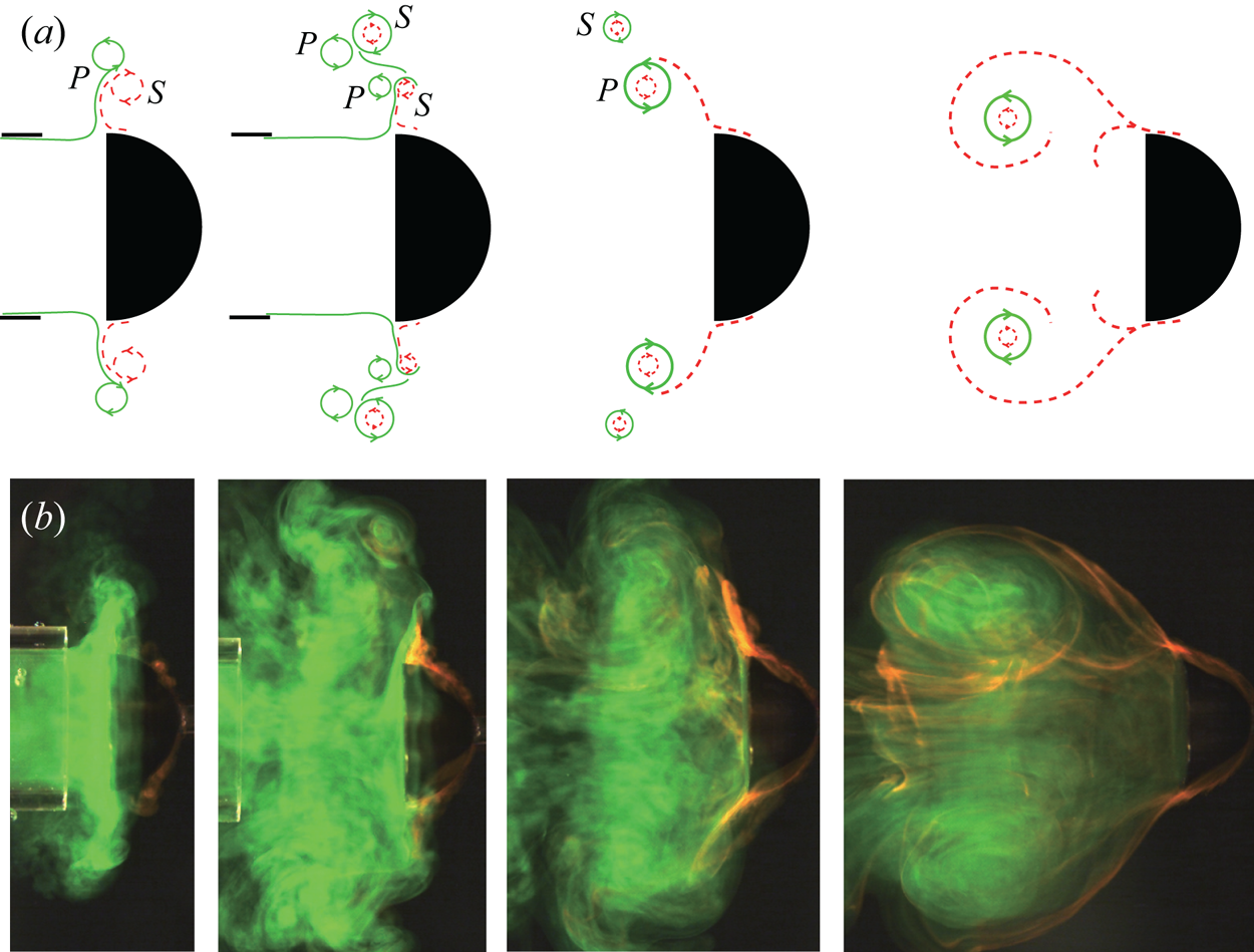
On the other hand, the spill mode is observed at the lowest  $U_{c}/U_{p}$. In this mode, the jet ejected by the piston impinges on the back surface of the cap and spills out radially to the surroundings (figure 3). The spilled jet expands radially, forming primary vortices (
 $P$ in figure 3a). They are accompanied by secondary vortices induced as the fluid near the surface of the cap is pulled up (
 $S$ in figure 3a) (Orlandi & Verzicco Reference Orlandi and Verzicco1993; Chu, Wang & Chang Reference Chu, Wang and Chang1995; New & Long Reference New and Long2015). Even after the formation of the secondary vortices, the axial jet from the cylinder continues to impinge on the cap and causes the repeated formation of primary and secondary vortices. This results in the dispersion of the fluid volume that is ejected from the cylinder and later entrained inside the radially expanding vortices. However, as the cap translates further forwards, enough room exists between the cap and the radially expanding vortices, and thus the latter eventually rolls up and forms a vortex ring-like structure; see
 $U_{p}t/L = 8.44$ in figure 3. During this process, the shear layer separated from the edge of the cap rolls up along the outside of the piston jet and merges together.
(a) Schematic diagram of the formation of the spill mode. The green solid line is the starting jet from the cylinder, and the red dashed line is the wake from the cap.  $P$ and
 $S$ denote primary vortices and secondary vortices, respectively. (b) Corresponding images from the two-dye experiment at four instants:
 $U_{p}t/L = [0.47, 2.15, 4.69, 8.44]$. Here
 $L/D = 4$,
 $U_{c}/U_{p} = 0.17$ and
 $Re_{p} = 3000$ (
 $U_{p} = 15.0\ \textrm {cm}\,\textrm {s}^{-1}$). See the supplementary movie for (b).

In the detached mode that appears for values of  $U_{c}/U_{p}$ greatest among the three modes, the translational speed of the cap is relatively high, so the cap is able to escape rapidly from the zone of the starting jet formed by the piston. Accordingly, the wake from the cap has minimal interaction with the piston jet soon after launch, and merger of the two flow structures is avoided (figure 4). Although the two flow structures form separately, their dynamics are not completely independent, and the wake from the cap still affects the formation of the jet from the cylinder. For the detached mode with relatively low
 $U_{c}/U_{p}$, these two vortices are close soon after the launch of the cap. Their interaction destabilizes the vortex from the cylinder, as a result of which the vortex quickly loses its form. Although not shown in the last image of figure 4(b), a vortex from the cylinder exists far behind the translating cap, and it becomes unstable faster than does a single vortex ring without the cap. The mutual interaction causing an unstable vortex seems to be less significant for cases with higher
 $U_{c}/U_{p}$ and greater
 $L/D$ up to
 $L/D = 4$, because the cap rapidly moves away from the piston jet and the longer piston stroke enables the formation of a stronger vortex that is resistant to destabilization.
(a) Schematic diagram of the formation of the detached mode. The green solid line is the starting jet from the cylinder, and the red dashed line is the wake from the cap. (b) Corresponding images from the two-dye experiment at three instants:  $U_{p}t/L = [0.21, 0.87, 1.95]$. Here
 $L/D = 4$,
 $U_{c}/U_{p} = 1.0$ and
 $Re_{p} = 3000$ (
 $U_{p} = 15.0\ \textrm {cm}\,\textrm {s}^{-1}$). See the supplementary movie for (b).

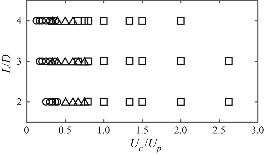
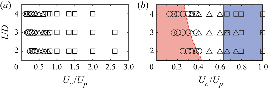
Figure 5 shows the distribution of the three vortex modes according to the velocity ratio  $U_{c}/U_{p}$ and stroke ratio
 $L/D$. As mentioned above, the spill mode is observed in the lowest
 $U_{c}/U_{p}$ range, followed by the attached mode and the detached mode as
 $U_{c}/U_{p}$ increases. It can be seen from figure 5 that
 $U_{c}/U_{p}$ is a more critical parameter in determining the vortex mode rather than
 $L/D$. Roughly, the transition from the spill mode to the attached mode and the transition from the attached mode to the detached mode are observed at
 $U_{c}/U_{p} \approx 0.3\text {--}0.4$ and
 $U_{c}/U_{p} \approx 0.7$, respectively. Although the features of the three vortex modes are distinct, it is difficult to clearly identify the transition from one mode to the other in the images from the dye experiment (figures 2–4). Quantitative criteria to distinguish the modes will be discussed in the following sections.
Distribution of the three modes of vortex interaction:  , spill mode;
 $\triangle$, attached mode;
 $\square$, detached mode.

3.2. Fluid entrainment
Before our analysis on fluid entrainment, we must point out that the definition of fluid entrainment in the present study is different from the conventional definition used in previous studies on vortex ring formation. According to the conventional definition, entrainment refers to the process in which surrounding ambient fluid is included into a vortex ring and is transported together with it (Maxworthy Reference Maxworthy1972). However, because this study is motivated by the transport of the spore particles discharged from a capsule (Sundberg Reference Sundberg2005, Reference Sundberg2010; Whitaker & Edwards Reference Whitaker and Edwards2010), we are interested in examining how effectively the fluid volume initially inside the cylinder is entrained inside the developing vortex structure and is transported following the cap. For this study, we define the entrainment fraction  $\eta$ as
 \begin{equation} \eta = \frac{\displaystyle \int_{V}\mathrm{d}V}{\dfrac{1}{4}{\rm \pi} D^2L}, \end{equation}
where the denominator is the total volume of fluid ejected from the cylinder during the entire stroke,  $D$ is the piston diameter and
 $L$ is the stroke length. The numerator is the volume of the ejected fluid that is entrained into the vortex structure and follows the translating cap.
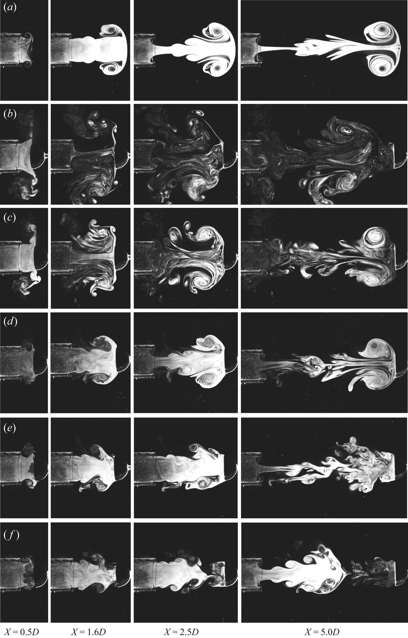
The velocity fields inside the cylinder are required for the trajectory of fluid initially inside the cylinder. However, because they were difficult to obtain in our PIV set-up, PIV was not appropriate to measure the entrainment fraction defined in (3.2). Moreover, although the velocity fields from PIV can be used to track the path of fluid elements outside the cylinder, it is sensitive to the spatial and temporal resolutions and accuracy of PIV, which may produce misleading results when we integrate flow velocity over a long time. Thus, as an alternative to PIV, LIF was used to evaluate the entrainment fraction. To quantify the amount of entrained fluid (the numerator in (3.2)), cross-sectional images taken from LIF experiments are used (figure 6). According to the histogram of the 8-bit greyscale LIF images, the background has an intensity up to 30, and the dyed fluid shows a mean intensity of approximately 100, with a bell-shaped distribution ranging dominantly between 50 and 150. An intensity value of 50 was chosen as the threshold value to ensure a clear contrast between the dyed fluid and the background fluid (water). Although the concentration of the dye is considered to quantify mixing in dye experiments, we neglect variations in concentration because the main purpose of the dye experiment is to track dyed fluid initially inside the cylinder, i.e. to determine whether or not dyed fluid exists at a certain position in the fluid domain. Using this threshold value, the raw LIF images were processed to give binary images, with intensity levels of 0 for the background and 255 for the dyed fluid.
Raw images of LIF experiments for  $L/D = 4$ and
 $Re_{p} = 3000$ (
 $U_{p} = 15\ \textrm {cm}\,\textrm {s}^{-1}$): (a) without a cap (vortex ring only); (b) spill mode (
 $U_{c}/U_{p} = 0.17$); (c) spill mode (
 $U_{c}/U_{p} = 0.25$); (d) attached mode (
 $U_{c}/U_{p} = 0.50$); (e) detached mode (
 $U_{c}/U_{p} = 0.67$); and (f) detached mode (
 $U_{c}/U_{p} = 1.00$). See the supplementary movies for (a) and (d).

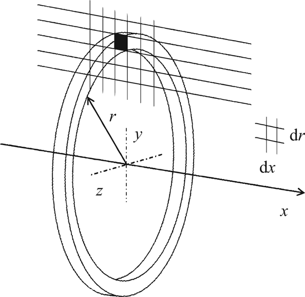
From the binary images, the three-dimensional volume of the dyed fluid is constructed as shown in figure 7 by assuming an axisymmetric distribution of the dyed fluid with respect to the  $x$ axis. This assumption of an axisymmetric distribution is reasonable because the vortex close to the cap can remain fairly symmetric, in particular during the initial formation process, and the formation of the major vortex structure is repeatable. Then, only for dyed fluid of intensity level 255,
 $\mathrm {d}V$ of (3.2) is obtained as
 \begin{equation} \mathrm{d}V = {\rm \pi}[(r+\mathrm{d}r)^2-r^2]\,\mathrm{d}x = {\rm \pi}[2r\,\mathrm{d}r+(\mathrm{d}r)^2]\,\mathrm{d}x, \end{equation}
where  $r$ is the radial coordinate, and
 $\mathrm {d}r$ and
 $\mathrm {d}x$ indicate the spatial resolution of the LIF images (figure 7). The volume of the dyed fluid, the numerator in (3.2), is computed twice, using pixels above the centreline (
 $x$ axis) and pixels below the centreline. The two values are then averaged to obtain the entrainment fraction
 $\eta$ in (3.2).
Schematic diagram of the coordinate system used for calculating the volume of dyed fluid from LIF images.

To validate our method using the LIF images, the conventional entrainment fraction obtained from Olcay & Krueger (Reference Olcay and Krueger2008) for a single isolated vortex ring was compared with that of a similar case without a cap from our experiments: the stroke ratio of 2, the piston speed of a trapezoidal profile and the Reynolds number of 1000 that is based on the piston velocity and the diameter of the nozzle exit. Note that the conventional entrainment fraction is defined as the ratio of the volume of the entrained ambient fluid to the volume of the vortex bubble. The conventional entrainment fraction of our experimental case has a mean value of 0.26, and it is similar to that of Olcay & Krueger (Reference Olcay and Krueger2008) with a mean value of 0.24, which confirms the reliability of our approach in evaluating the volume of the dyed fluid. Our mean value is slightly larger because the time of observation used to average the conventional entrainment fraction is more than two times larger, compared to figure 9 of Olcay & Krueger (Reference Olcay and Krueger2008). The additional entrainment of the ambient fluid occurs as the propagating vortex ring slowly expands over time.
In the image processing to compute the volume of the dyed fluid, a primary factor for uncertainty is the threshold value of dye concentration. When we varied the threshold value between 45 and 55, we were able to track the dyed fluid even for low concentration. However, inside vortex core regions where mixing of dyed fluid and entrained ambient fluid occurs, the distinction in concentration between the two fluids was not clear. For the threshold range 45–55, such uncertainty accounted for the maximum 7 % difference in the entrainment fraction from the result of the threshold value 50 used for this study.
As the dyed fluid is transported through the medium, it is diffused and dissolved into the surroundings. However, according to Olcay & Krueger (Reference Olcay and Krueger2008) and Bouremel & Ducci (Reference Bouremel and Ducci2017), the change in the concentration of dye due to diffusion is negligible because the Schmidt number of fluorescein dye in water is  $Sc = \nu /\kappa = 2370$. Here, the Wilke–Chang correlation (Wilke & Chang Reference Wilke and Chang1955) is used to obtain the diffusion coefficient
 $\kappa$ of the dye. Since the Schmidt number of fluorescein is higher than 1000, the dyed fluid is capable of tracking fluid motion, but not vorticity diffusion (Green Reference Green1995). Therefore, the change in
 $\eta$ is mostly due to a decrease in the concentration of dyed fluid. This decrease in concentration is caused by the break-up of the vortex structure and mixing with the fluid medium, which leads to dissolution of the dye in the latter. Accordingly,
 $\eta$ is expected to maintain a high value for a stable fluid structure, whereas it decreases dramatically for an unstable fluid structure.
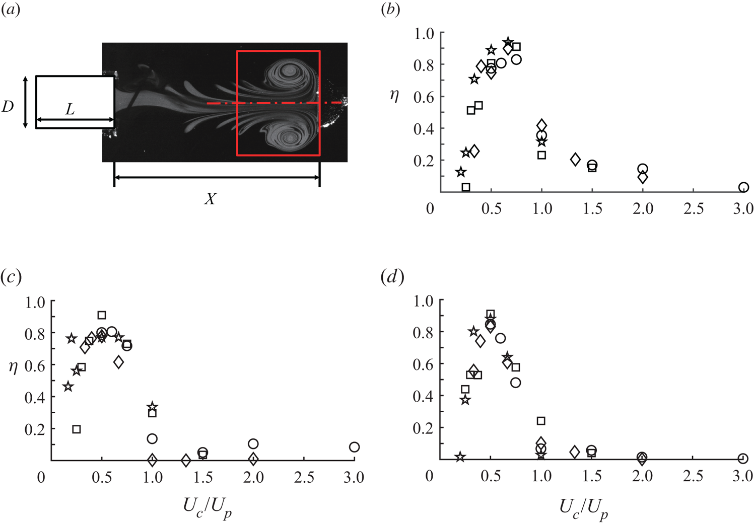
The entrainment fractions newly defined in (3.2) for this study are compared at the instant when the cap passes  $X = 4D$ for different stroke ratios (figure 8); from now on, the entrainment fraction defined in (3.2) will be used consistently instead of the conventional definition used in previous studies. The domain used to compute the entrainment volume of the fluid for the numerator in (3.2) is subjective. In this study, this domain is confined to be
 $1.5D \times 2.5D$ behind the cap (figure 8a). For the attached mode that is our main interest (figure 6d), this domain is sufficiently large for the main vortex structure to be included in the numerator in (3.2). We confirmed that the entrainment fraction shown in figure 8 also had a similar trend when computed in the earlier phases,
 $X = 2D$ and
 $3D$; note that
 $\eta$ is time-dependent. However, at
 $X = 2D$ and
 $3D$, the vortex structure behind the cap is not fully developed or clearly separated from the piston jet, in contrast to
 $X = 4D$. To compare the magnitude of the entrainment fraction in the three vortex modes distinctly, we chose
 $X = 4D$ for figure 8.
(a) Entrainment fraction  $\eta$ (3.2) is computed when the cap passes
 $X = 4D$. The region used to compute the volume of dyed fluid (red box) is set as
 $1.5D \times 2.5D$. (b–d) Entrainment fraction as a function of velocity ratio for (b)
 $L/D = 2$, (c)
 $L/D = 3$ and (d)
 $L/D = 4$, with
 $Re_{p} = 1000$ (
 ), 1500 (
 $\diamond$), 2000 (
 $\square$) and 3000 (
 $\star$) (corresponding to
 $U_{p} = 5.0$, 7.5, 10.0 and
 $15.0\ \textrm {cm}\,\textrm {s}^{-1}$ respectively).

Notably, the effect of  $L/D$ on the magnitude of
 $\eta$ is insignificant in the entire range of
 $U_{c}/U_{p}$ (figure 8). For all three stroke ratios (
 $L/D = 2$, 3 and 4),
 $\eta$ has a peak reaching roughly 0.8 at
 $U_{c}/U_{p}$ near 0.5. Relatively high values of
 $\eta$ are observed in the
 $U_{c}/U_{p}$ range between approximately 0.3 and 0.7, which coincides with the
 $U_{c}/U_{p}$ range of the attached mode (figure 5). This result is in good agreement with what we observe in figures 2 and 6(d): a significant portion of the fluid volume from the cylinder follows the cap in the attached mode. In the attached mode, fluid transport benefits from the coupling with the forward-moving cap, and it can be regarded as the most favourable vortex mode in terms of fluid transport.
In the spill mode, as the velocity ratio  $U_{c}/U_{p}$ increases from zero, the amount of fluid spilling out radially decreases, and the amount of fluid entrained inside the vortex structure increases: compare figures 6(b) and 6(c) with different velocity ratios in the spill mode. This corresponds to the growth in the entrainment fraction for the spill mode until the transition to the attached mode near
 $U_{c}/U_{p} = 0.3\text {--}0.4$ (figure 8).
On the other hand, in the detached mode, a dramatic fall in the entrainment fraction occurs near  $U_{c}/U_{p} = 0.7$. Indeed, figure 6(e) for
 $U_{c}/U_{p} = 0.67$ shows a remarkable reduction in the entrained fluid volume, which is followed by a more drastic decrease in figure 6(f) for
 $U_{c}/U_{p} = 1.00$; both belong to the detached mode. One might think that, for the detached mode with very high
 $U_{c}/U_{p}$, the vortex generated from the cylinder could transport a large amount of the dyed fluid comparable to that of a single vortex ring with no cap, because the effect of the rapidly translating cap on the piston jet is negligible during its formation and thereafter; i.e. the vortex from the cylinder behaves like a single isolated vortex ring in a still fluid medium. However, as mentioned in § 3.1, in the detached mode under such a condition, the vortex structure can be easily destabilized after a short time by the wake that remains behind the rapidly translating cap, thereby losing its ability to transport the dyed fluid volume for a long distance. For example, compare the shape of the jet from the cylinder on the fourth column of figure 6(a) for a single vortex ring and figure 6(f) for the detached mode with
 $U_{c}/U_{p} = 1.0$.
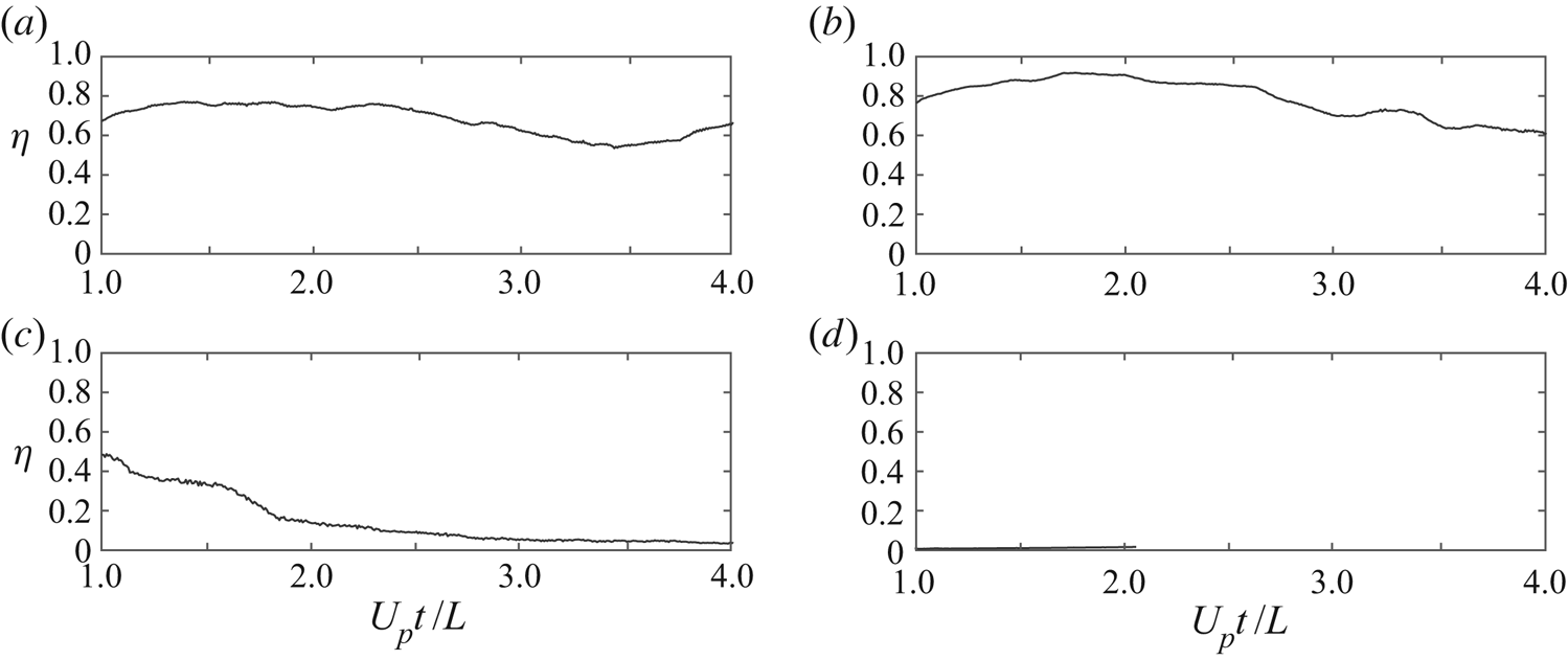
As well as  $\eta$ at a fixed position
 $X=4D$ in figure 8, the time histories of
 $\eta$ are compared for the three vortex modes in figure 9. To compute the volume of entrained fluid, the same domain size,
 $1.5D \times 2.5D$, as that of figure 8(a) is used for
 $X \geq 1.5D$; and, for
 $X < 1.5 D$, the
 $x$ directional length of the domain is adjusted to be the same as the distance
 $X$. Because both
 $U_{p}$ and
 $L$ are critical in the transport of the fluid volume ejected by the piston, they are chosen over
 $U_{c}$ and
 $D$ as the characteristic velocity and length to non-dimensionalize time as
 $U_{p}t/L$; this dimensionless time has been used in figures 2–4 and 6. This definition also makes the piston stroke finish at
 $U_{p}t/L = 1.0$ uniformly for all cases.
Time history of the entrainment fraction  $\eta$ for
 $L/D = 4$ and
 $Re_{p} = 3000$ (
 $U_{p} = 15.0\ \textrm {cm}\,\textrm {s}^{-1}$): (a) without a cap (vortex ring only); (b) attached mode (
 $U_{c}/U_{p} = 0.50$); (c) spill mode (
 $U_{c}/U_{p} = 0.17$); and (d) detached mode (
 $U_{c}/U_{p} = 1.00$).

The time histories of  $\eta$ offer a quantitative criterion to distinguish the vortex modes, without relying on observation from figures 2–4. The entrainment fraction before the stroke ends (
 $U_{p}t/L = 1.0$) tends to include not only the piston jet following the cap motion but also the piston jet dispersing radially for spill mode cases as shown in figure 3. Thus, for a better comparison of the entrainment fraction, a cut-off time of
 $U_{p}t/L = 1.0$ is used. In this study, the entrainment fraction after
 $U_{p}t/L = 1.0$ is considered important because the trends of the entrainment fraction among the three vortex modes are clearly distinguished thereafter.
The entrainment fractions of the attached mode and the case without a cap exhibit a similar pattern (figure 9a,b). For the no-cap case, although the distance  $X$ from the cylinder end to the cap cannot be defined, the same domain size as that of the other cases is used. In each case of figure 9(a,b), a plateau in
 $\eta$ appears after
 $U_{p}t/L = 1.0$ as the vortex structure reaches a steady state. The maximum
 $\eta$ of the attached mode is comparable to that of the no-cap case:
 $\eta = 0.9$ for the attached mode and
 $\eta = 0.8$ for the no-cap case. Meanwhile, for the spill mode, the radially expanded vortices, primary and secondary ones, dissipate into the surroundings, and only a small amount of ejected fluid remains inside the propagating vortex structure, which results in a lower
 $\eta$ (figure 9c). For the detached mode (figure 9d), as expected, only a small fraction of the dyed fluid follows the cap, and the entrainment fraction remains very low during the entire stroke time.
The stroke ratio  $L/D$ is not as significant as the velocity ratio
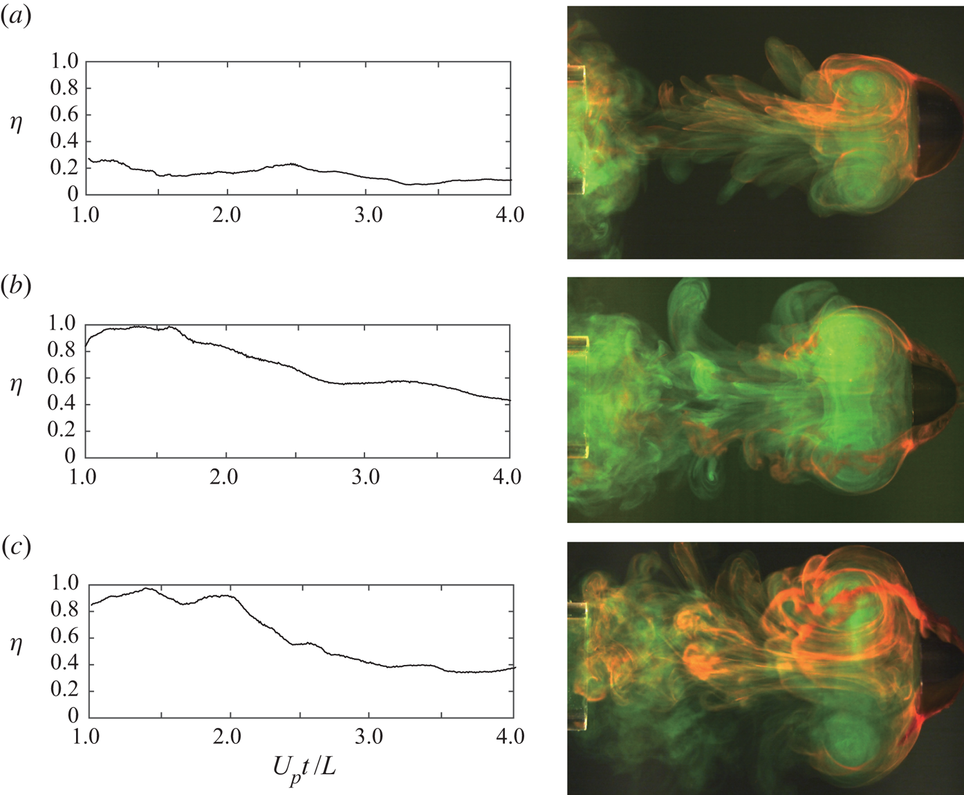
 $U_{c}/U_{p}$ in determining the vortex modes (figure 5). However, a stroke-dependent behaviour of the entrainment fraction is observed in the spill mode. Generally, the size of the vortex structure following the cap grows with
 $L/D$ (figure 10). For
 $L/D = 2$ in figure 10(a), when a vortex structure is formed after initial spill-out, the piston stops ejecting fluid, thereby limiting the volume entrained into the vortex structure. The amount of dyed fluid spilling out is relatively large compared with the entrained volume, and the maximum
 $\eta$ is limited to below
 $\eta = 0.3$. Meanwhile, for a longer stroke (
 $L/D = 3$ and 4), which means a longer ejection time for the same
 $U_{p}$, a greater amount of dyed fluid can be fed into the developing vortex structure, enlarging its size (figure 10b,c). Consequently, as
 $L/D$ increases, the vortex structure of the spill mode tends to become similar to that of the attached mode. Moreover, the maximum entrainment fraction is comparable to that of the attached mode; the appendix provides the time history plots of the entrainment fraction for the cases near a transition from the spill mode to the attached mode. However, in contrast to the attached mode, the cases of
 $L/D = 3$ and 4 for the spill mode exhibit a notable drop in
 $\eta$ after
 $U_{p}t/L = 1.0$ (figure 10b,c).
Time history of entrainment fraction  $\eta$ for spill mode cases with
 $U_{c}/U_{p}$ = 0.25 and
 $Re_{p} = 3000$ (
 $U_{p} = 15.0\ \textrm {cm}\,\textrm {s}^{-1}$): (a)
 $L/D = 2$; (b)
 $L/D = 3$; and (c)
 $L/D = 4$. For each case, an image from the two-dye experiment is provided:
 $(a)\,\, U_{p}t /L = 6.33, (b)\,\, U_{p}t /L = 4.15, (c)\,\, U_{p}t /L = 3.16.$

The boundary between the vortex modes can be defined in terms of entrainment fraction. Although all cases are not provided here, the time history of the entrainment fraction shows two distinct trends: the cases for which the entrainment fraction remains in the range of  $\eta = 0.7$ to 0.9 after the piston stops (
 $U_{p}t/L = 1.0$) until the cap reaches
 $X = 4D$ and the cases for which the entrainment fraction falls below
 $\eta \approx 0.6$. Admittedly, the classification of the vortex modes using two-dye visualization was difficult due to similarity in the vortex structure at the transitional regions: i.e.
 $U_{c}/U_{p} = 0.3$ to 0.4 between spill mode and attached mode and
 $U_{c}/U_{p} \approx 0.7$ between attached mode and detached mode. However, regarding the entrainment fraction, setting a threshold value of
 $\eta = 0.7$ can divide the two different trends of entrainment fraction and clearly distinguish the vortex modes. The formation of a stable vortex structure occurs only in the attached mode, which is a necessary condition in maintaining a high entrainment fraction (figure 9b). The case with the entrainment fraction above the threshold is defined as the attached mode, and this criterion was used to obtain the vortex mode distribution in figure 5.
3.3. Circulation
In this section, the characteristics of the three vortex modes are discussed with regard to the circulation of the vortex structure. The circulation is defined as
 \begin{equation} \varGamma = \int_A \omega \,\mathrm{d}A = \sum_{A} \omega {\rm \Delta} x{\rm \Delta} y. \end{equation}
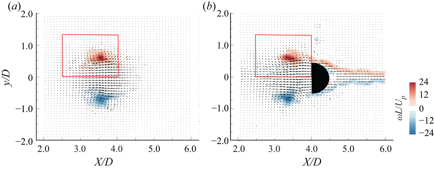
Similar to figure 8(a), the area used to compute the circulation  $\varGamma$ is set to enclose the vortex structure near the cap (figure 11). In figure 11(a), the red box of dimensions
 $1.50D \times 1.25D$ denotes the area
 $A$ used to compute the circulation. Only the upper region above the
 $x$ axis is considered; and
 ${\rm \Delta} x$ and
 ${\rm \Delta} y$ correspond to the spatial resolution of the vorticity field obtained from PIV. To avoid including noise in (3.4), vorticity with an absolute value less than
 $1\ \textrm {s}^{-1}$ is neglected. The computed circulation
 $\varGamma$ is non-dimensionalized by piston velocity
 $U_{p}$ and stroke length
 $L$, thus
 $\varGamma /(U_{p} L)$.
Velocity vectors and vorticity contours for  $L/D = 3$ and
 $Re_{p} = 2000$ (
 $U_{p} = 10\ \textrm {cm}\,\textrm {s}^{-1}$): (a) without a cap (vortex ring only); (b) attached mode (
 $U_{c}/U_{p}= 0.5$). The flow field is captured when the cap passes through
 $X = 4D$ for the attached mode and at the same dimensionless time for the no-cap case:
 $U_{p}t/L = 2.67$. The red box of dimensions
 $1.5D\times 1.25D$ indicates the area used to compute circulation (3.4).

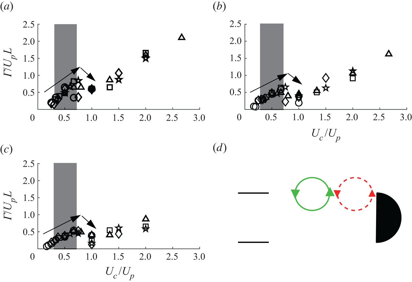
In figure 12, circulation at  $X = 4D$ is presented, which is the same location of the cap as in figure 8. The circulations for various cases in figures 12(a–c) show a similar trend regardless of the stroke ratio
 $L/D$. The relatively small value of the circulation in the spill mode is due to the loss of momentum of the jet flow during the impingement onto the cap, which results in a vortex structure with weaker vorticity behind the cap. For a given
 $U_{p}$, as the cap speed
 $U_{c}$ (and
 $U_{c}/U_{p}$) increases, the effect of impingement is reduced, and thus a gradual growth in circulation occurs in the
 $U_{c}/U_{p}$ range of the spill mode.
Dimensionless circulation  $\varGamma /(U_{p}L)$ at
 $X = 4D$ for (a)
 $L/D = 2$, (b)
 $L/D = 3$ and (c)
 $L/D = 4$, with
 $Re_{p} = 3000$ (
 ), 2000 (
 $\diamond$), 1500 (
 $\square$), 1000 (
 $\star$) and 750 (
 $\triangle$), corresponding to
 $U_{p} = 15.0$, 10.0, 7.5, 5.0 and
 $3.75\ \textrm {cm}\,\textrm {s}^{-1}$, respectively. (d) Schematic diagram of counteracting vortices in the detached mode near
 $U_{c}/U_{p} = 1.0$.

In § 3.1, we pointed out that a fully developed vortex structure in the attached mode propagated at the same speed as that of the cap. In the attached mode, for a given  $U_{p}$, an increase in the cap speed
 $U_{c}$ contributes to accelerating the vortex structure to follow the cap. Accordingly, a steady increase in circulation is observed in figure 12 as
 $U_{c}/U_{p}$ increases in the region of the attached mode highlighted as grey between
 $U_{c}/U_{p} \approx 0.3$ and
 $0.7$. In the attached mode as well as the spill mode, the dimensionless circulation exhibits a linear relation with the velocity ratio up to
 $U_{c}/U_{p}\approx 0.7$, making it difficult to identify the transition between the spill mode and the attached mode from figure 12.
Meanwhile, the circulation drops after the peak near  $U_{c}/U_{p} = 0.7$ (figure 12), indicating the transition from attached mode to detached mode. In the detached mode, the two vortices from the two sources, the cylinder and the cap, have a certain distance between them (figure 12d). Owing to mutual interaction, one vortex attenuates the strength of the other because fluids rotate in the opposite directions in the region between the vortices, leading to a drop in the circulation. The decrease in circulation continues up to
 $U_{c}/U_{p} = 1.0$. As
 $U_{c}/U_{p} > 1.0$ in the detached mode, the influence of the jet from the cylinder on the formation of the vortex structure behind the cap becomes less. The rise in the circulation after
 $U_{c}/U_{p} = 1.0$ is attributed mostly to an increase in
 $U_{c}$ and the consequent feeding of stronger vorticity from the cap.
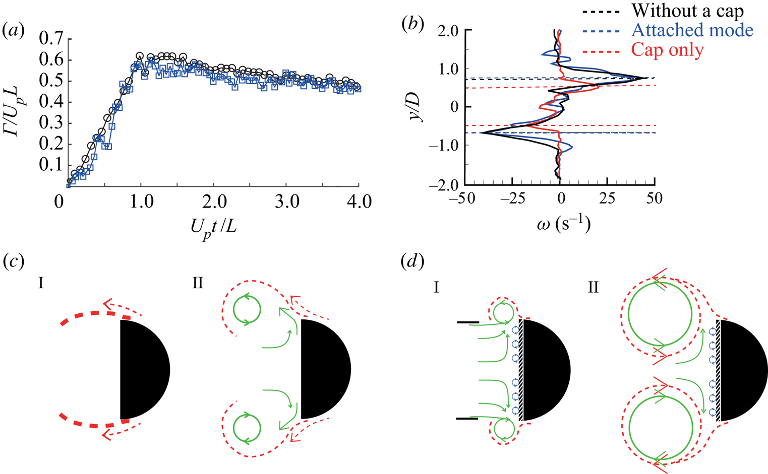
In addition to the overall flow structure (figure 6a,d), the velocity and vorticity fields are similar as well between the no-cap case and the attached mode of  $U_{c}/U_{p} = 0.5$ for the same stroke length and piston velocity (figure 11); the propagation speed of the vortex structure is also similar in these two cases. Consistent with these observations, the dimensionless circulation of the attached mode shows only minor deviation from that of the no-cap case, even after the stroke ends at
 $U_{p}t/L = 1$ (figure 13a). The circulation grows linearly until the piston stops, which is followed by a plateau. The vortex structures retain their integrity without losing their forms and maintain a high circulation value with only minor reductions until
 $U_{p}t/L = 4.0$. Even after the stroke ends, the vorticity profiles remain similar between these two cases (figure 13b). In addition, the case for which only the cap translates without piston motion (
 $U_{p} = 0$) is included in figure 13(b). While the locations of positive and negative peak vorticities are located approximately
 $1.0D$ apart in the cap-only case, in the other two cases, the distances between the peaks are greater, approximately
 $1.4D$, and the magnitudes of the peaks become greater as well.
(a) Time history of dimensionless circulation  $\varGamma /(U_{p} L)$ and (b) vorticity profile for the case without a cap (vortex ring only,
 $U_{p} = 10\ \textrm {cm}\,\textrm {s}^{-1}$, black) and for the attached mode (
 $U_{c} = 5\ \textrm {cm}\,\textrm {s}^{-1}$,
 $U_{c}/U_{p} = 0.5$, blue):
 $L/D =3$. The case in which only the cap moves without the piston stroke (
 $U_{c} = 5\ \textrm {cm}\,\textrm {s}^{-1}$, red) is also included in (b). Vorticity is plotted along a line passing through the peak vorticity of the vortex structure. For the attached mode and cap-only cases, the vorticity plot is captured when the cap passes
 $X = 4D$:
 $U_{p}t/L = 2.67$. The same
 $U_{p}t/L = 2.67$ is used for the case without a cap. The horizontal dashed lines in (b) mark the locations of the vorticity peaks. (c) Schematic diagram of the shear layer development at the edge of the cap for (I) the cap-only case and (II) the attached mode. The red dashed line and green solid circle denote the shear layer from the cap and the vortex from the cylinder, respectively. (d) Schematic diagram during (I) the formation of the vortex structure and (II) its propagation after development. The hatched area on the back surface of the cap denotes the region where the vorticity of opposite sign (blue circle) is produced.

Although the vorticity generated from the cap surface is fed into the vortex structure in the attached mode, the circulations are almost the same in figure 13(a), implying that the strength of the vortex structure behind the cap is not simply the superposition of the two sources: the vortex ring from the piston and the wake from the cap. While the translation of a cap produces considerable vorticity of its own for the cap-only case (figure 13b), the feeding of the vorticity generated on the cap into the separated shear layer (vortex structure) is small for the attached mode. This difference in the strength of the shear layer can be explained by the work of Xia & Mohseni (Reference Xia and Mohseni2017) on the generation of a shear layer from a finite-angle trailing edge, in which an analytical model on the strength of the shear layer is derived. The difference in flow velocity between the upper surface and lower surface at the trailing edge of an airfoil was shown to be directly proportional to the amount of circulation fed into the shear layer. In the reference frame fixed with the translating cap, the cap-only case (figure 13c-I) shows a greater difference in flow velocity at the cap edge between the flow moving over the cap and the flow in the vicinity of the back surface of the cap: i.e. a greater difference in flow velocity across the shear layer separated from the cap edge. Meanwhile, for the attached mode case, the jet from the piston impinges onto the back surface of the cap. Sequentially, the impinging jet turns around, changing its direction, and radially expands, which leads to a reduction in the difference in flow velocity across the shear layer (figure 13c-II). Therefore, the amount of net vorticity (circulation) separated from the cap edge becomes much smaller in the attached mode compared to the cap-only case.
A reduction in the strength of the shear layer can also be explained via the perspective of vorticity production. When the jet from the cylinder interacts with the back surface of the cap, the vorticity of the opposite sign is generated on the back surface due to the friction on the surface (figure 13d). This vorticity of the opposite sign eventually merges into the main vortex structure, causing a reduction in the circulation of the vortex structure. That is, the production of vorticity of the opposite sign on the back surface can offset the addition of vorticity from the front surface of the cap. In the attached mode, the merge of the wake structure and the vortex ring is responsible for the small fluctuation of vorticity with positive and negative signs outside the core, which is observed from the vorticity distribution of the attached mode in figure 13(b).
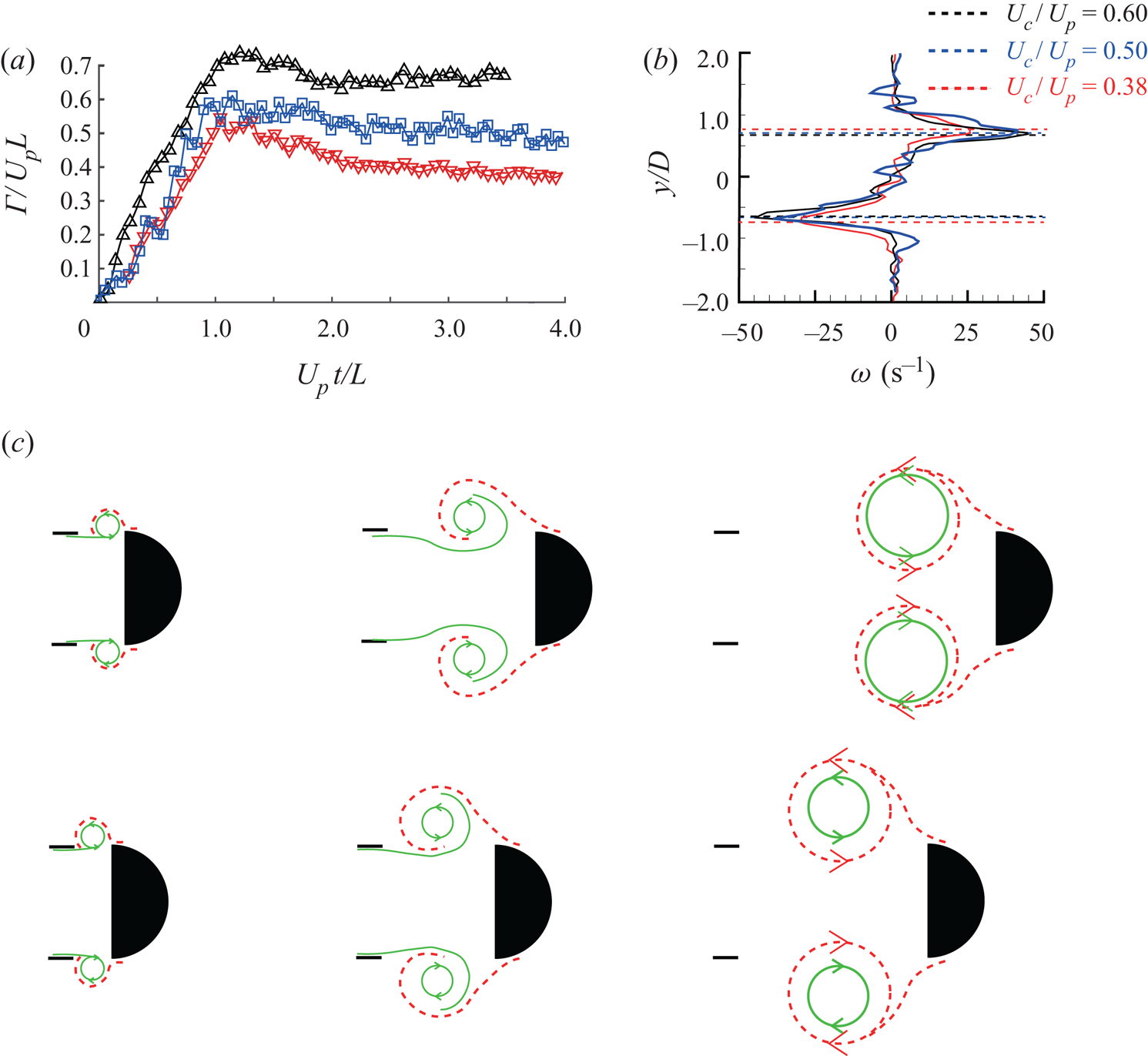
In figure 14(a), for the three attached mode cases with the same  $U_{p}$ (
 $U_{c}/U_{p} = 0.38$, 0.50 and 0.60), the magnitude of circulation shows a linear relationship with the translational speed
 $U_{c}$ of the cap; approximately 20 % increase in circulation for
 $U_{c}/U_{p} = 0.60$ and 25 % decrease for
 $U_{c}/U_{p} = 0.38$, compared to the
 $U_{c}/U_{p} = 0.50$ case. Consistently, the vorticity profile in figure 14(b) shows the larger magnitude of peak vorticity for the higher cap velocity. Because of the linear relationship between the circulation and the cap velocity for the attached mode, the vortex structure can propagate with a similar velocity to the cap velocity, as mentioned in § 3.1. On the other hand, in the attached mode, the
 $y$ directional distance between the two peaks of vorticity magnitude increases slightly with the decrease in the cap velocity (figure 14b):
 $1.3D$ for
 $U_{c}/U_{p} = 0.60$ and
 $1.5D$ for
 $U_{c}/U_{p} = 0.38$. This trend is caused by the radial expansion of the vortex during the formation phase as the velocity ratio decreases (figure 14c). Eventually, the radial expansion of the vortex becomes more prominent as the velocity ratio drops into the regime of spill mode (figure 3).
(a) Time history of dimensionless circulation  $\varGamma /(U_{p} L)$ and (b) vorticity profile for three attached mode cases:
 $U_{c}/U_{p} = 0.60$, black;
 $U_{c}/U_{p} = 0.50$, blue; and
 $U_{c}/U_{p} = 0.38$, red. Here
 $L/D =3$ and
 $Re_{p} = 2000$ (
 $U_{p} = 10\ \textrm {cm}\,\textrm {s}^{-1}$). (b) Vorticity plotted along a line passing through the peak vorticity of the vortex structure when the cap passes
 $X = 4D$. The horizontal dashed lines in (b) mark the locations of the vorticity peaks. (c) Schematic diagram of the vortex structure for
 $U_{c}/U_{p} = 0.60$ and 0.38. The red dashed line and green solid line denote the shear layer from the cap and the vortex from the cylinder, respectively.

3.4. Analytical prediction of vortex mode transition
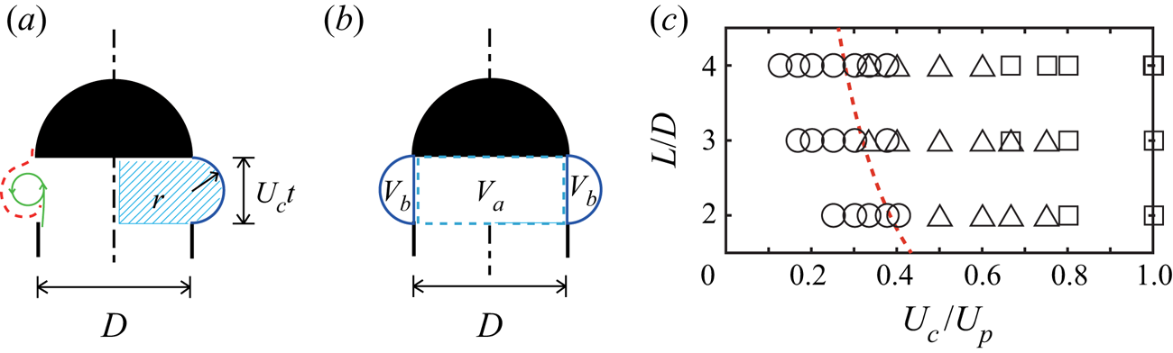
Based on our findings in the preceding sections, we provide simple analytical models to predict the transitions between the vortex modes: i.e. the boundaries between spill mode and attached mode, and between attached mode and detached mode (figure 5). Let us first consider the transition between the spill mode and the attached mode. Before the stroke ends, the entrainment of the ambient fluid into the vortex is negligible as seen from figure 9 of Olcay & Krueger (Reference Olcay and Krueger2008), which is less than 10 % of the fluid ejected from the cylinder. We assume that, in the early stage of launch, which is defined as the stage until the piston stroke ends, the shape of the vortex structure can be simplified as shown in the left half of figure 15(a), in which green and red lines denote the jet from the cylinder and the wake from the cap, respectively (figures 2–4). The volume of fluid ejected by the piston during time  $t$ from the start is
 $V_{p} = \frac {1}{4}{\rm \pi} D^2 U_{p} t$. We assume that the volumetric capacity
 $V_{c}$ of the vortex at time
 $t$ is approximated as the volume of an axisymmetric rounded disk shape as shown hatched in blue in the right half of figure 15(a). Then, the volumetric capacity
 $V_{c}$ is the sum of
 $V_{a}$ and
 $V_{b}$, i.e.
 $V_{c} = V_{a} + V_{b}$, where
 $V_{a}$ and
 $V_{b}$ are shown in figure 15(b). Here
 $V_{a}$ is the cylindrical volume displaced by the translation of the cap, and
 $V_{b}$ is the volume of the outer half of a torus used to model the radial expansion of the vortex due to roll-up. Using
 $r=\frac {1}{2}U_{c}t$ in figure 15(a),
 $V_{b}$ can be written with the same variables as
 $V_{a}$:
 \begin{gather} V_{a} = \frac{1}{4}{\rm \pi} D^2 U_{c} t, \end{gather}
 \begin{gather}V_{b} = \frac{4}{3} {\rm \pi} r^3 + \frac{1}{2}{\rm \pi}^2 Dr^2 = \frac{1}{6} {\rm \pi} U_{c}^3t^3 + \frac{1}{8}{\rm \pi}^2DU_{c}^2t^2. \end{gather}
(a,b) Schematic diagrams of the analytical model used to predict the transition between the spill mode and the attached mode. (c) Boundary (red dashed line) between the spill mode and the attached mode, which is obtained by solving (3.7).

The volumetric capacity  $V_{c}$ of the vortex should be greater than the fluid volume
 $V_{p}$ ejected by the piston (
 $V_{c} > V_{p}$) in order to contain all ejected fluid volume. For
 $V_{c} < V_{p}$, the fluid should spill out of the volume of the axisymmetric rounded disk shape. The condition
 $V_{c}\ ( = V_{a}+V_{b}) = V_{p}\ ( = \frac {1}{4}{\rm \pi} D^2 U_{p} t)$ can be expressed as a third-order polynomial equation in
 $U_{c}$ and
 $t$:
 \begin{equation} \frac{1}{2}{\rm \pi} \left[\frac{1}{3}U_{c}^3t^3+\frac{1}{4}{\rm \pi} DU_{c}^2t^2+\frac{1}{2}D^2(U_{c}-U_{p})t \right]=0. \end{equation}
If  $V_{c}$ is greater than
 $V_{p}$ at some instant before the piston stroke ends, the ejected fluid is well contained thereafter: this is the attached mode. Accordingly, by substituting the time limit when the piston stroke ends,
 $t = L/U_{p}$, into (3.6) and dividing the equation by
 $D^3$, we obtain
 \begin{equation} \frac{1}{3}\left(\frac{U_{c}}{U_{p}}\right)^3\left(\frac{L}{D}\right)^2+ \frac{{\rm \pi}}{4}\left(\frac{U_{c}}{U_{p}}\right)^2 \left(\frac{L}{D}\right)+\frac{1}{2}\left(\frac{U_{c}}{U_{p}}-1\right)=0. \end{equation}
For a given  $L/D$, (3.7) provides the value of
 $U_{c}/U_{p}$ on the boundary between the spill mode and the attached mode (red dashed line in figure 15c). On the right side of the boundary,
 $V_{c}$ can be greater than
 $V_{p}$ before the time limit
 $t = L/U_{p}$, and the attached mode occurs accordingly. Although this simple model does not deal with complicated vortex dynamics in detail, it predicts the transition boundary reasonably well. In § 3.2 and figure 10, we reported that, for the spill mode, an increase in
 $L/D$ resulted in the formation of a vortex structure similar to that observed in the attached mode. In the same context, with increasing
 $L/D$, the transition from the spill mode to the attached mode is observed in the lower critical
 $U_{c}/U_{p}$, and our model (3.7) is able to capture this trend (figure 15c).
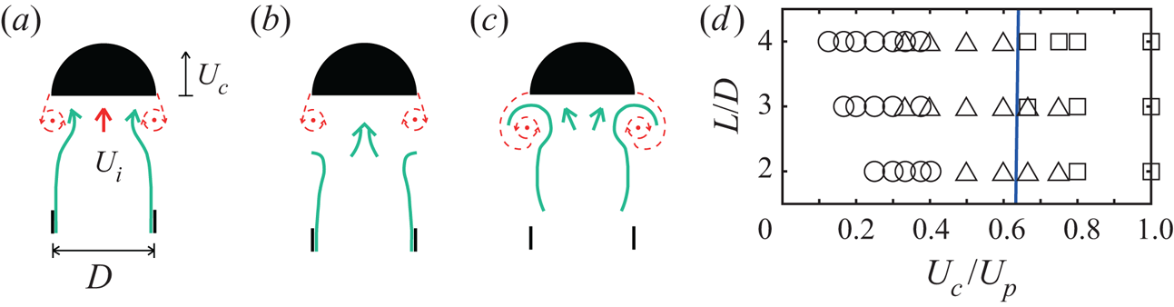
Next, for the transition between the attached mode and the detached mode, another model should considered (figure 16). To induce the fluid ejected by the piston to be entrained inside the merged vortex structure in the attached mode, in the early phase of launch, the piston jet needs to reach the back side of the translating cap. If the speed of the cap is too large, then the piston jet is unable to enter the region where the shear layer from the cap rolls up. Consequently, merger with the wake from the cap cannot be achieved, eventually leading to the formation of the two discrete vortices from the piston and the cap (detached mode), as shown in figure 16(b). However, if the cap speed is sufficiently low, the piston jet can reach the cap and continue to feed momentum and vorticity. Then, the two vortices can eventually merge, giving rise to the attached mode (figure 16c).
(a) Illustration of the piston jet merging into the wake of the cap;  $U_{i}$ (red arrow) is the velocity induced by the wake at the centre of the wake. (b,c) Schematic diagrams of vortex formation (b) in the detached mode and (c) in the attached mode. In (a–c), the jet from the cylinder is indicated by the green solid lines and the wake from the cap by the red dashed lines. (d) Boundary (blue solid line) between the attached mode and the detached mode, which is obtained by (3.11).

We need to quantify velocity components in order to elaborate the above argument. For a single isolated vortex ring with a thin vortex core in a static fluid medium, the self-induced flow velocity  $U_{i}$ at the centre of the vortex ring on the
 $x$ axis (
 ${r} = 0)$ is expressed, using the Biot–Savart law for a circular vortex filament of a finite core thickness
 $a$ (Saffman Reference Saffman1993), as
 \begin{equation} U_{i} = \frac{\varGamma R^2}{2 (R^2+a^2)^{3/2}}, \end{equation}
where  $\varGamma$ is the strength of the vortex filament and
 $R$ is the radius of the vortex ring. Note that this induced velocity at the centre of the vortex ring is different from the self-induced propagation speed of the vortex ring. The core thickness
 $a$ is obtained from PIV data and is approximated to be 0.2
 $R$. By assuming a very thin vortex filament, i.e.
 $a\rightarrow 0$, (3.8) can be simplified to
 \begin{equation} U_{i} = \frac{\varGamma}{2R}. \end{equation}
Because the difference in the magnitude of  $U_{i}$ between (3.8) and (3.9) is just within approximately
 $5\,\%$ for our models, (3.9) is chosen as an expression of
 $U_{i}$ for simplicity. If we assume that the wake generated by the cap has the form of a thin vortex ring of radius
 $\frac {1}{2}D$ as shown in figure 13(b), the induced velocity at the centre of the wake from the cap can be approximated as
 $U_{i} = \varGamma /D$ from (3.9) (red arrow in figure 16a). On the other hand, the velocity of the piston jet column is similar to the piston velocity
 $U_{p}$ in the initial phase of launch. If
 $U_{p}$ remains larger than
 $U_{i}$ before the piston stroke ends, the piston jet is able to reach the wake of the cap, and the vortices can merge, leading to the attached mode. Otherwise, the vortices cannot merge, and the detached mode ensues.
According to our experimental results for the cases in which only the cap translates without piston motion, the circulation of the wake generated by the cap grows and reaches its maximum before the piston stroke ends. We use this maximum circulation value as the upper limit of  $\varGamma$, which yields the upper limit of
 $U_{i}\ (=\varGamma / D)$ as well. The maximum
 $\varGamma$ is found to be in a linear relationship with the translational velocity of the cap:
 $\varGamma _{max} \approx 1.6U_{c}D$ for all cases in which only the cap translates without piston motion. Then, the maximum velocity induced by the wake at the centre is given by
 \begin{equation} U_{i,max} = \frac{\varGamma}{D} \approx 1.6 U_{c}. \end{equation}
From our experiments, we confirmed that the actual maximum induced velocity at the centre of the wake behind the cap ranged between  $1.4U_{c}$ and
 $1.6U_{c}$, which is close to (3.10). By equating
 $U_{p}$ and
 $U_{i,max}$, the boundary between the attached mode (
 $U_{p} > U_{i,max}$) and the detached mode (
 $U_{p} < U_{i,max}$) can be obtained in terms of the velocity ratio:
 \begin{equation} U_{c}/U_{p} \approx 0.63. \end{equation}
In (3.11), the velocity ratio on the transition boundary is constant regardless of any change in  $L/D$ (figure 16d).
Figure 17 shows the vortex mode distribution obtained by the experiments and the mode boundaries obtained by the analytical models. Although our analytical approach relies on some ad hoc assumptions and does not consider complex vortex interactions, it offers a moderate prediction of the transitions with only slight deviation and can predict that the value of  $U_{c}/U_{p}$ at the mode transition is merely affected by
 $L/D$.
(a) Figure 5 replotted. (b) Vortex mode distribution for the velocity ratio range  $U_{c}/U_{p} = 0\text {--}1.0$, along with the two boundaries obtained theoretically (figures 15c and 16d). Red and blue regions correspond to the spill mode and the detached mode, respectively.

4. Concluding remarks
We investigated how the vortices generated from two different sources interact with each other by using a piston–cylinder apparatus coupled with a forward-moving cap, which is motivated by the launch process of a Sphagnum spore capsule. By varying the stroke length and the translational speeds of the cap and the piston, the mutual interaction of the two vortices is divided into three distinct modes: a spill mode, an attached mode and a detached mode. The distribution of these three modes is determined mainly by the ratio of cap speed and piston speed. The vortex structures for the spill and detached modes are not adequate to transport the fluid initially inside the cylinder, following the translating cap, which ends up a low entrainment fraction. On the other hand, the vortex structure of the attached mode is able to retain a high entrainment fraction throughout its propagation. In the attached mode, the coupling of the jet from the cylinder and the wake from the cap results in the formation of a stable vortex structure very similar to that of a single vortex ring generated by the piston only.
In this study, we focused on the vortex interactions that may be present in the early stage of spore launch. The attached mode observed in this study shows a superior capability for fluid transport compared with the other modes, implying that the formation of the stable vortex structure is desirable for transporting spore particles over a longer distance in the actual discharge process of a spore capsule. Although the actual launch mechanism of spores obviously differs from our simplified experimental model, the analysis on vortex formation under the influence of a translating forward-moving body offers insight into the vortex dynamics and transport processes that occur in the spore launch process. Based on our results, we conjecture that vortex formation in the attached mode is realized to enhance the capability of spore transport. The experimental verification of this speculation with Sphagnum remains a topic for future work.
The present study used a scaled-up mechanical model and prescribed the motions of the cap and the piston to facilitate changes in design parameters and focus on vortex dynamics. In the future, we plan to conduct experiments with a more realistic model and shooting mechanism using the impulsive discharge of compressed air. We hope that the findings of this study and of future work will contribute to understanding the fluid mechanics of the ballistic processes in nature or nature-inspired applications.
Acknowledgements
This research was supported by the Basic Science Research Program through the National Research Foundation of Korea (NRF) funded by the Ministry of Science and ICT (NRF-2017R1E1A1A01074704) and the Human Resources Program in Energy Technology of the Korea Institute of Energy Technology Evaluation and Planning (KETEP) granted financial resources from the Ministry of Trade, Industry and Energy, Republic of Korea (no. 20204030200050).
Declaration of interests
The authors report no conflict of interest.
Supplementary movies
Supplementary movies are available at https://doi.org/10.1017/jfm.2020.633.
Appendix
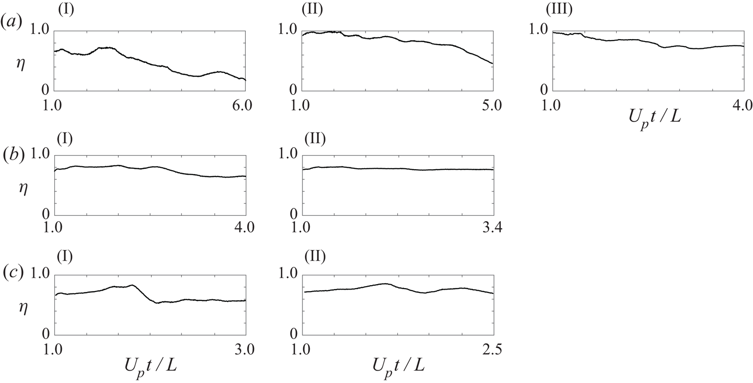
Additional time history plots of an entrainment fraction are provided to show that a transition from the spill mode to the attached mode differs by the stroke ratio  $L/D$ (figure 18). According to our analysis about the effect of the stroke ratio on fluid entrainment in § 3.2, a longer stroke length enables the roll-up of the vortex structure even after the initial spill, and the entrainment fraction is higher for cases with a longer stroke length for given piston and cap velocities. Thus, for large
 $L/D$ cases, the transition between the spill mode and the attached mode can occur at a smaller
 $U_{c}/U_{p}$ as demonstrated in figure 5.
Time history of entrainment fraction  $\eta$ for cases near a transition from the spill mode to the attached mode with
 $Re_{p} = 1500$ (
 $U_{p} = 7.5\ \textrm {cm}\,\textrm {s}^{-1}$). (a) For
 $L/D = 2$: (I) spill mode
 $U_{c}/U_{p} = 0.33$; (II) spill mode
 $U_{c}/U_{p} = 0.40$; (III) attached mode
 $U_{c}/U_{p} = 0.50$. (b) For
 $L/D = 3$: (I) spill mode
 $U_{c}/U_{p} = 0.33$; (II) attached mode
 $U_{c}/U_{p} = 0.40$. (c) For
 $L/D = 4$: (I) spill mode
 $U_{c}/U_{p} = 0.33$; (II) attached mode
 $U_{c}/U_{p} = 0.40$. The range of the dimensionless time
 $U_{p}t/L$ is different for each panel because data were obtained from the end of the piston stroke (
 $U_{p}t/L = 1.0$) until the cap reaches
 $X = 4D$.