1 Introduction
The onset of natural convection due to transient diffusion of heat or solutes through a porous medium has been studied extensively for its roles in carbon sequestration (Riaz & Cinar Reference Riaz and Cinar2014), oil recovery (Aziz, Bories & Combarnous Reference Aziz, Bories and Combarnous1973; Goyal, Pichler & Meiburg Reference Goyal, Pichler and Meiburg2007), subsurface contaminant transport (Hassanzadeh, Pooladi-Darvish & Keith Reference Hassanzadeh, Pooladi-Darvish and Keith2009) and the dynamics of miscible fluid interfaces (Fernandez et al. Reference Fernandez, Kurowski, Petitjeans and Meiburg2002). In purely fluid media, similar convection occurs in heat transfer devices (Goldstein Reference Goldstein1959; Elder Reference Elder1968), geophysical flows (Wooding, Tylers & White Reference Wooding, Tylers and White1997) and Rayleigh–Bénard–Marangoni convection (Doumenc et al. Reference Doumenc, Boeck, Guerrier and Rossi2010). Transient convection in porous media also attracts considerable theoretical attention because it is governed by a unique non-autonomous stability problem for which modal stability theory is invalid (Foster Reference Foster1965; Ben, Demekhin & Chang Reference Ben, Demekhin and Chang2002; Rapaka et al. Reference Rapaka, Chen, Pawar, Stauffer and Zhang2008). It is consequently often studied as a ‘toy problem’ to investigate fundamental questions concerning the stability of transient flows (Daniel, Tilton & Riaz Reference Daniel, Tilton and Riaz2013; Tilton, Daniel & Riaz Reference Tilton, Daniel and Riaz2013; Tilton & Riaz Reference Tilton and Riaz2014). Another model problem for investigating the stability of transient flows is the onset of centrifugal instabilities in transient circular Couette flow (Neitzel, Kirkconnell & Little Reference Neitzel, Kirkconnell and Little1995). In comparison to that problem, convection due to transient diffusion in porous media is driven by buoyancy, and has nonlinear mechanisms arising from the advection–diffusion equation, but not the momentum equation. The presence of the porous medium also provides a physically natural framework for continuously forcing perturbations, which is the primary focus of the current study.
The current study investigates the onset of transient convection in the context of carbon sequestration, not only for its application, but also as a classic problem for which we can reconsider how the onset of transient convection has been modelled to date. When supercritical CO
 $_{2}$
is injected in a subsurface saline aquifer, the buoyant CO
 $_{2}$
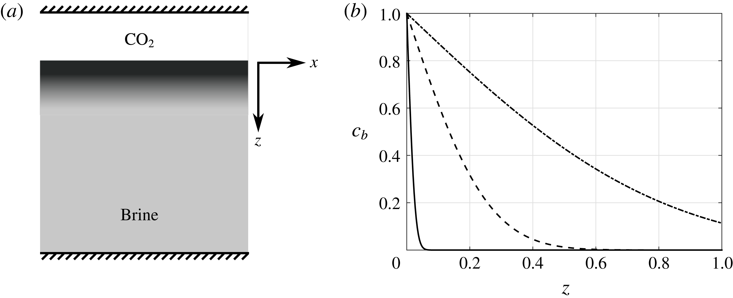
accumulates in a horizontal layer bounded by cap rock above, and brine below, as illustrated in figure 1(a). With time, CO
 $_{2}$
dissolves into the underlying brine and diffuses downwards. As the density of the brine increases with CO
 $_{2}$
concentration, a gravitational instability causes the formation of finger-like structures that convect CO
 $_{2}$
-rich brine downward. Predicting the onset of this instability is key to evaluating potential sequestration sites.
(a) Sketch, not to scale, of the idealized two-dimensional aquifer geometry considered in the current study. (b) The transient base state, see (3.3), at times
 $t=0.1$
(solid line),
 $t=1$
(dashed line) and
 $t=100$
(dash-dotted line).

To date, the linear stability of transient convection has been studied using primarily quasi-steady modal (QSM) methods and non-modal initial value problem (IVP) methods. Both approaches have focused on the onset of instability due to the growth of perturbations introduced to the concentration field. This has produced considerable debate (see Slim & Ramakrishnan Reference Slim and Ramakrishnan2010; Daniel et al.
Reference Daniel, Tilton and Riaz2013; Tilton et al.
Reference Tilton, Daniel and Riaz2013). First, although both methods predict that perturbations become linearly unstable at a finite critical time
 $t=t_{c}$
, they predict widely varying results for
 $t_{c}$
depending on the norm used to measure growth. Second, QSM and IVP methods often produce unphysical perturbation structures for which the sum of the base state and perturbation produces unphysical negative concentrations. Third, IVP methods show that optimal perturbations must be initiated at a finite time
 $t_{p}$
to maximize perturbation growth. Finally, although studies often focus on finding perturbation structures that minimize the critical time
 $t_{c}$
for linear instability, the results may be of limited practical use. This is because the perturbation structures that minimize
 $t_{c}$
are different from those that trigger the ensuing onset time
 $t_{on}$
for nonlinear convection (Tilton & Riaz Reference Tilton and Riaz2014). The onset time
 $t_{on}$
is arguably more important than
 $t_{c}$
when evaluating sequestration sites, because
 $t_{on}$
marks the time where nonlinear mechanisms cause an increase in the rate of CO
 $_{2}$
dissolution (Hewitt, Neufeld & Lister Reference Hewitt, Neufeld and Lister2013). Conventional QSM and IVP methods cannot predict
 $t_{on}$
because they only capture linear instability mechanisms.
We propose a new IVP approach to modelling the linear stability and onset of nonlinear convection in transient diffusive layers. The approach has two unique features. First, while previous IVP studies focus on the impulse response to perturbations introduced in the concentration field, we consider that diffusion through porous media is continuously perturbed by spatial porosity variations. Second, while previous analyses focus on the critical time
 $t_{c}$
for instability, we focus on the onset time
 $t_{on}$
for nonlinear convection. For this purpose, we show that
 $t_{on}$
can be accurately predicted using a simple asymptotic expansion that allows us to perform parametric studies that would be prohibitively costly using direct numerical simulations (DNS).
Though we refer to our method as ‘new’ in the context of buoyancy-driven convection, it builds closely on previous literature. Jhaveri & Homsy (Reference Jhaveri and Homsy1982) investigated convection in heated fluid layers using a nonlinear IVP that subjects the momentum equation to continuous random forcing. Subsequently, Chen, Neitzel & Jankowski (Reference Chen, Neitzel and Jankowski1987) used a similar approach to study unsteady circular Couette flow. To our knowledge, onset of nonlinear convection due to porosity perturbations was first demonstrated by Pau et al. (Reference Pau, Bell, Pruess, Almgren, Lijewski and Zhang2010) using DNS. Building on the works above, we develop a much simpler expansion method that expands about small porosity perturbations. The expansion procedure is motivated by a similar expansion developed by Tilton & Riaz (Reference Tilton and Riaz2014) for the case of the impulse response to initial concentration perturbations.
Our study makes three main contributions. (i) We show that when transient diffusion is perturbed through the porosity field, instability occurs immediately (
 $t_{c}=0$
). The instability does not require an initial perturbation to the concentration field, and is insensitive to the initial time
 $t_{p}$
at which the IVP is initiated. This brings into question previous literature that characterizes instability in terms of
 $t_{c}$
and
 $t_{p}$
, including work by the current author (Daniel et al.
Reference Daniel, Tilton and Riaz2013; Tilton et al.
Reference Tilton, Daniel and Riaz2013; Tilton & Riaz Reference Tilton and Riaz2014). (ii) We show that when systems are continuously perturbed by porosity variations, perturbations to the concentration field arise naturally and are physically realizable. The perturbation structures are similar to those suggested by Ben et al. (Reference Ben, Demekhin and Chang2002), Riaz et al. (Reference Riaz, Hesse, Tchelepi and Orr2006) and Daniel et al. (Reference Daniel, Tilton and Riaz2013), but different from those of Rapaka et al. (Reference Rapaka, Chen, Pawar, Stauffer and Zhang2008) and Slim & Ramakrishnan (Reference Slim and Ramakrishnan2010). (iii) We show that for spatially periodic porosity perturbations, optimal combinations of wavelengths minimize
 $t_{on}$
. Moreover, even small porosity perturbations of the order of
 $10^{-7}$
are sufficient to trigger the onset of nonlinear convection, and thereby trigger a regime of increased CO
 $_{2}$
flux, within a time scale comparable to those observed in previous studies. This observation may be significant, because studies of convection in heterogeneous media often ignore porosity variations by arguing that they are typically small (De Wit & Homsy Reference De Wit and Homsy1997; Daniel, Riaz & Tchelepi Reference Daniel, Riaz and Tchelepi2015).
2 Governing equations
As in most previous QSM and IVP analyses (see review in Tilton et al.
Reference Tilton, Daniel and Riaz2013), we consider two-dimensional convection in a saline aquifer of infinite horizontal extent. The aquifer is bounded by supercritical CO
 $_{2}$
at
 $z=0$
and impermeable rock at
 $z=H$
, where
 $z$
points in the direction of gravity, as in figure 1(a). We assume the aquifer is locally isotropic, but with a spatially varying porosity
 $\unicode[STIX]{x1D719}(\boldsymbol{x})$
expressed mathematically as
 $$\begin{eqnarray}\unicode[STIX]{x1D719}=\langle \unicode[STIX]{x1D719}\rangle \widehat{\unicode[STIX]{x1D719}}(\boldsymbol{x}),\quad \langle \unicode[STIX]{x1D719}\rangle =\frac{1}{HL}\int _{0}^{H}\int _{0}^{L}\unicode[STIX]{x1D719}\,\text{d}x\,\text{d}z,\end{eqnarray}$$
where
 $\langle \unicode[STIX]{x1D719}\rangle$
denotes the spatially averaged porosity over
 $H$
and some length
 $L$
in the
 $x$
-direction. A small spatial porosity perturbation is introduced by expressing
 $\widehat{\unicode[STIX]{x1D719}}(\boldsymbol{x})$
as
 $$\begin{eqnarray}\widehat{\unicode[STIX]{x1D719}}=1+\unicode[STIX]{x1D716}\widetilde{\unicode[STIX]{x1D719}}(\boldsymbol{x}),\end{eqnarray}$$
where
 $\unicode[STIX]{x1D716}\ll 1$
is some measure of the perturbation magnitude, to be defined later. The spatial variation is given by
 $\widetilde{\unicode[STIX]{x1D719}}(\boldsymbol{x})$
, which by definition has a zero average,
 $\langle \widetilde{\unicode[STIX]{x1D719}}\rangle =0$
.
We consider an initially quiescent brine with uniform density
 $\unicode[STIX]{x1D70C}_{0}$
and zero CO
 $_{2}$
concentration. We model CO
 $_{2}$
dissolution by assuming that at time
 $t=0$
, saturated brine is supplied at
 $z=0$
with constant concentration
 $C_{sat}$
and density
 $\unicode[STIX]{x1D70C}_{sat}>\unicode[STIX]{x1D70C}_{0}$
. Because the density difference
 $\unicode[STIX]{x0394}\unicode[STIX]{x1D70C}=\unicode[STIX]{x1D70C}_{sat}-\unicode[STIX]{x1D70C}_{0}$
is of order 1 % (Nomeli, Tilton & Riaz Reference Nomeli, Tilton and Riaz2014), we model transport using the volume-averaged continuity, Darcy, and advection–diffusion equations with the Boussinesq approximation (Whitaker Reference Whitaker1999). We non-dimensionalize the problem as in Riaz et al. (Reference Riaz, Hesse, Tchelepi and Orr2006) using the length
 $H$
, buoyancy velocity
 $U=K\unicode[STIX]{x0394}\unicode[STIX]{x1D70C}g/\unicode[STIX]{x1D707}$
, time
 $\langle \unicode[STIX]{x1D719}\rangle H/U$
and concentration
 $C_{1}$
. The non-dimensionalized governing equations may then be written as,
 $$\begin{eqnarray}\frac{\unicode[STIX]{x2202}u}{\unicode[STIX]{x2202}x}+\frac{\unicode[STIX]{x2202}w}{\unicode[STIX]{x2202}z}=0,\quad \boldsymbol{v}+\unicode[STIX]{x1D735}p-c\boldsymbol{e}_{z}=0,\end{eqnarray}$$
 $$\begin{eqnarray}\widehat{\unicode[STIX]{x1D719}}\frac{\unicode[STIX]{x2202}c}{\unicode[STIX]{x2202}t}+\underbrace{u\frac{\unicode[STIX]{x2202}c}{\unicode[STIX]{x2202}x}+w\frac{\unicode[STIX]{x2202}c}{\unicode[STIX]{x2202}z}}_{advection}=\underbrace{\frac{1}{Ra}\unicode[STIX]{x1D735}\boldsymbol{\cdot }(\widehat{\unicode[STIX]{x1D719}}\unicode[STIX]{x1D735}c)}_{dispersion},\end{eqnarray}$$
 $$\begin{eqnarray}c|_{z=0}=1,\quad \left.\frac{\unicode[STIX]{x2202}c}{\unicode[STIX]{x2202}z}\right|_{z=1}=w|_{z=0}=w|_{z=1}=0,\quad c|_{t=0}=0,\end{eqnarray}$$
where
 $\boldsymbol{e}_{z}$
is the unit vector in the
 $z$
-direction,
 $\boldsymbol{v}=[u\;w]^{\text{T}}$
is the non-dimensional velocity vector,
 $c$
is the non-dimensional concentration and the non-dimensional pressure is defined as
 $p=(p^{\ast }-\unicode[STIX]{x1D70C}gz)/(\unicode[STIX]{x0394}\unicode[STIX]{x1D70C}gh)$
, where
 $p^{\ast }$
is the dimensional pressure. The Rayleigh number is defined as
 $Ra=UH/(\langle \unicode[STIX]{x1D719}\rangle {\mathcal{D}})$
. The advection and dispersion terms in (2.4) have been labelled to facilitate discussion in § 3. Equation (2.5) applies a no-flux condition at
 $z=1$
, and no penetration at
 $z=0$
and
 $1$
. Note that the second equation in (2.3) can be combined with the first to produce the simpler form
 $\unicode[STIX]{x1D6FB}^{2}w=\unicode[STIX]{x2202}^{2}c/\unicode[STIX]{x2202}x^{2}$
.
Several comments regarding our formulation are warranted. First, though we begin by non-dimensionalizing our problem with respect to the length scale
 $H$
, we will show in § 4.3 that the length scale
 $\langle \unicode[STIX]{x1D719}\rangle {\mathcal{D}}/U$
is more appropriate. Second, equations (2.1)–(2.5) can be rigorously derived by averaging the pore-scale continuity, Stokes and advection–diffusion equations over a small averaging volume of radius
 $r$
(Bear Reference Bear1972; Whitaker Reference Whitaker1999). The derivation assumes
 $r$
is much larger than a typical pore scale, and that the volume-averaged flow fields vary over length scales larger than
 $r$
. Although care should be taken to satisfy these constraints,
 $r$
is rarely defined in practice, except in pore-scale studies. In the current study, we take the approach of considering porosity variations that vary over length scales comparable to the depth,
 $\unicode[STIX]{x1D6FF}$
, of the transient diffusive boundary layer at
 $t=t_{on}$
, see (3.3) in § 3.
Third, we note that porosity variations usually lead to variations in the permeability and dispersion coefficient. In past literature, the effects of heterogeneous porosity, permeability and dispersion are typically studied separately. For example, numerous studies allow the permeability to vary spatially, while the porosity and dispersion coefficients are maintained constant (De Wit & Homsy Reference De Wit and Homsy1997; Daniel et al.
Reference Daniel, Riaz and Tchelepi2015). In contrast, our approach provides a natural framework for exploring how the functional dependence of
 $K$
and
 ${\mathcal{D}}$
on
 $\unicode[STIX]{x1D719}$
affects onset of convection. For the purposes of the current study, however, we prefer to isolate the effects of porosity perturbations so as to simplify the presentation of our expansion and facilitate comparison with previous QSM and IVP analyses of homogeneous aquifers. Moreover, the functional dependence of
 $K$
and
 ${\mathcal{D}}$
on the porosity remains a field of study. For the case of permeability, Verma & Pruess (Reference Verma and Pruess1988) cite widely varying relationships of the form
 $K\sim \unicode[STIX]{x1D719}^{b}$
where
 $1\leqslant b\leqslant 6$
. Examples of more recent work include Delfiner (Reference Delfiner2007), Liu et al. (Reference Liu, Zhang, Yi and Wang2013) and Tang & McDonough (Reference Tang and Mcdonough2016).
3 Methodology
3.1 Asymptotic expansion
QSM and IVP studies typically derive linear stability equations by assuming all perturbation flow fields are infinitesimally small. We prefer to formally expand the governing nonlinear equations (2.3)–(2.5) about the amplitude
 $\unicode[STIX]{x1D716}$
of the porosity perturbations. In this manner, we systematically recover the zero-order transient base state, first-order linear stability problem and a second-order correction for nonlinear effects. We begin by seeking a solution to (2.3)–(2.5) as a regular asymptotic expansion,
 $$\begin{eqnarray}c(\boldsymbol{x},t)\approx c_{b}(\boldsymbol{x},t)+\unicode[STIX]{x1D716}c_{1}(\boldsymbol{x},t)+\unicode[STIX]{x1D716}^{2}c_{2}(\boldsymbol{x},t),\end{eqnarray}$$
with similar expansions for
 $u$
and
 $w$
. The choice of subscript for
 $c_{b}$
will be evident soon. As in Tilton & Riaz (Reference Tilton and Riaz2014), we do not pursue a multiscale expansion because the regular expansion (3.1) is particularly efficient, and because the problem becomes strongly nonlinear such that a multiscale expansion may not offer much advantage.
Substituting (3.1) into equations (2.3)–(2.5) and gathering terms of equal order in
 $\unicode[STIX]{x1D716}$
produces the following equations at order
 $\unicode[STIX]{x1D716}^{0}$
,
 $$\begin{eqnarray}\frac{\unicode[STIX]{x2202}u_{b}}{\unicode[STIX]{x2202}x}+\frac{\unicode[STIX]{x2202}w_{b}}{\unicode[STIX]{x2202}z}=0,\quad \unicode[STIX]{x1D6FB}^{2}w_{b}=\frac{\unicode[STIX]{x2202}^{2}c_{b}}{\unicode[STIX]{x2202}x^{2}},\quad \frac{\unicode[STIX]{x2202}c_{b}}{\unicode[STIX]{x2202}t}+u_{b}\frac{\unicode[STIX]{x2202}c_{b}}{\unicode[STIX]{x2202}x}+w_{b}\frac{\unicode[STIX]{x2202}c_{b}}{\unicode[STIX]{x2202}z}=\frac{1}{Ra}\unicode[STIX]{x1D6FB}^{2}c_{b},\end{eqnarray}$$
subject to conditions (2.5). As there is no perturbation at order
 $\unicode[STIX]{x1D716}^{0}$
, the zero-order solution must describe transient diffusion through quiescent fluid in a homogeneous aquifer,
 $$\begin{eqnarray}\boldsymbol{v}_{b}=0,\quad c_{b}(z,t)=1-\frac{4}{\unicode[STIX]{x03C0}}\mathop{\sum }_{n=1}^{\infty }\frac{1}{2n-1}\sin \left[\left(n-\frac{1}{2}\right)\unicode[STIX]{x03C0}z\right]\exp \left[-\left(n-\frac{1}{2}\right)^{2}\frac{\unicode[STIX]{x03C0}^{2}t}{Ra}\right].\end{eqnarray}$$
Figure 1(b) shows
 $c_{b}(z,t)$
for
 $Ra=500$
at times
 $t=0.1$
, 1 and 100. It is worth stressing that because we formally expand (3.1) about
 $\unicode[STIX]{x1D716}$
, the zero-order solution (3.3) recovers the same transient base state
 $c_{b}(z,t)$
considered in previous linear stability analyses of convection in homogeneous isotropic aquifers.
Orders
 $\unicode[STIX]{x1D716}^{1}$
and
 $\unicode[STIX]{x1D716}^{2}$
are governed by the following linear initial value problems (IVP),
 $$\begin{eqnarray}\frac{\unicode[STIX]{x2202}u_{j}}{\unicode[STIX]{x2202}x}+\frac{\unicode[STIX]{x2202}w_{j}}{\unicode[STIX]{x2202}z}=0,\quad \unicode[STIX]{x1D6FB}^{2}w_{j}=\frac{\unicode[STIX]{x2202}^{2}c_{j}}{\unicode[STIX]{x2202}x^{2}},\quad \frac{\unicode[STIX]{x2202}c_{j}}{\unicode[STIX]{x2202}t}+w_{j}\frac{\unicode[STIX]{x2202}c_{b}}{\unicode[STIX]{x2202}z}-\frac{1}{Ra}\unicode[STIX]{x1D6FB}^{2}c_{j}=F_{j},\end{eqnarray}$$
 $$\begin{eqnarray}F_{1}=-\widetilde{\unicode[STIX]{x1D719}}\frac{\unicode[STIX]{x2202}c_{b}}{\unicode[STIX]{x2202}t}+\frac{\unicode[STIX]{x2202}}{\unicode[STIX]{x2202}z}\left[\frac{\widetilde{\unicode[STIX]{x1D719}}}{Ra}\frac{\unicode[STIX]{x2202}c_{b}}{\unicode[STIX]{x2202}z}\right],\quad F_{2}=-\widetilde{\unicode[STIX]{x1D719}}\frac{\unicode[STIX]{x2202}c_{1}}{\unicode[STIX]{x2202}t}-\boldsymbol{v}_{1}\boldsymbol{\cdot }\unicode[STIX]{x1D735}c_{1}+\unicode[STIX]{x1D735}\boldsymbol{\cdot }\left(\frac{\widetilde{\unicode[STIX]{x1D719}}}{Ra}\unicode[STIX]{x1D735}c_{1}\right),\end{eqnarray}$$
where the index
 $j$
denotes the order. Because the base-state solution satisfies the non-homogeneous boundary condition
 $c_{b}=1$
at
 $z=0$
, equations (3.4)–(3.5) must satisfy the homogeneous boundary and initial conditions
 $$\begin{eqnarray}c_{j}|_{z=0}=\left.\frac{\unicode[STIX]{x2202}c_{j}}{\unicode[STIX]{x2202}z}\right|_{z=1}=w_{j}|_{z=0}=w|_{z=1}=0,\quad c_{j}|_{t=0}=0.\end{eqnarray}$$
To interpret equations (3.4)–(3.5) physically, we first note that when
 $F_{1}=0$
, the first-order problem recovers the same linear stability equations considered in most previous analyses. In this case, one requires a non-zero initial condition for
 $c_{1}$
to initiate instability. The instability mechanism can be interpreted physically by considering the vorticity equation formed from the curl of the Darcy equation (2.3),
 $$\begin{eqnarray}\unicode[STIX]{x1D714}=\unicode[STIX]{x1D735}c\times \boldsymbol{e}_{z}=-\frac{\unicode[STIX]{x2202}c}{\unicode[STIX]{x2202}x}.\end{eqnarray}$$
Equation (3.7) indicates that vorticity is generated by a misalignment between the concentration gradient and the gravity vector (Tan & Homsy Reference Tan and Homsy1988). In previous analyses, this misalignment is triggered by introducing concentration perturbations that vary in the horizontal direction. Although not pursued here, instability could also be triggered by forcing the boundary conditions at
 $z=0$
to mimic perturbations originating from the interface, as is common in Hele-Shaw cells (Kneafsey & Pruess Reference Kneafsey and Pruess2010).
In our approach, the misalignment in (3.7) is triggered by the forcing term
 $F_{1}$
in (3.5). The first term in
 $F_{1}$
arises due to the unsteady term
 $\widehat{\unicode[STIX]{x1D719}}(\unicode[STIX]{x2202}c/\unicode[STIX]{x2202}t)$
in the advection–diffusion equation (2.4). To interpret the mechanism physically, we note that
 $\widehat{\unicode[STIX]{x1D719}}(\unicode[STIX]{x2202}c/\unicode[STIX]{x2202}t)$
represents the unsteady accumulation of solutes in an averaging volume due to the difference between the advective and diffusive fluxes of solutes across the volume’s surface. From (2.4), we see that for fixed fluxes, regions of low porosity will experience greater magnitudes of
 $\unicode[STIX]{x2202}c/\unicode[STIX]{x2202}t$
than regions of high porosity. The second term in
 $F_{1}$
arises due to the dispersion term on the right-hand side of (2.4). This triggers instability due to horizontal variations in dispersion brought on by variations in
 $\widetilde{\unicode[STIX]{x1D719}}(x,z)$
.
When we account for the fact that the base-state equation (3.2) reduces to
 $\unicode[STIX]{x2202}c_{b}/\unicode[STIX]{x2202}t=(1/Ra)(\unicode[STIX]{x2202}^{2}c_{b}/\unicode[STIX]{x2202}z^{2})$
, we see that
 $F_{1}$
reduces to only one term,
 $$\begin{eqnarray}F_{1}=\frac{1}{Ra}\frac{\unicode[STIX]{x2202}\widetilde{\unicode[STIX]{x1D719}}}{\unicode[STIX]{x2202}z}\frac{\unicode[STIX]{x2202}c_{b}}{\unicode[STIX]{x2202}z},\end{eqnarray}$$
such that instability is triggered only by dispersion effects. Considering the second-order forcing
 $F_{2}$
, we see similar mechanisms to those in
 $F_{1},$
and a new term,
 $\boldsymbol{v}_{1}\boldsymbol{\cdot }\unicode[STIX]{x1D735}c_{1}$
, representing nonlinear interactions arising from the convective term in (2.4).
Expansion (3.1) has some similarities to an expansion developed by De Wit & Homsy (Reference De Wit and Homsy1997) in a study of viscous fingering. In that case, the authors expanded to first order about the magnitude of spatial permeability perturbations. They then performed a second expansion in terms of a flow field perturbation. The resulting double expansion was studied using quasi-steady methods. In contrast, we perform a single expansion about
 $\unicode[STIX]{x1D716}$
to second order, and use a non-modal IVP approach.
3.2 Fourier analysis
Equations (3.4)–(3.5) can be further simplified by decomposing the porosity perturbation
 $\widetilde{\unicode[STIX]{x1D719}}(x,z)$
in a sum of porosity perturbations varying sinusoidally in the
 $x$
-direction as
 $$\begin{eqnarray}\widetilde{\unicode[STIX]{x1D719}}(x,z)=(\text{e}^{\text{i}kx}+\text{e}^{-\text{i}kx})f(z)=2\cos (kx)f(z),\end{eqnarray}$$
where
 $f(z)$
is a real-valued shape function and
 $k$
is the horizontal wavenumber. A solution to the first-order problem can then be found in the separable form
 $$\begin{eqnarray}\left[\begin{array}{@{}c@{}}c_{1}\\ u_{1}\\ w_{1}\end{array}\right]=2\left[\begin{array}{@{}c@{}}\widehat{c}_{1}(z,t)\cos (kx)\\ \text{i}\widehat{u}_{1}(z,t)\sin (kx)\\ \widehat{w}_{1}(z,t)\cos (kx)\end{array}\right],\end{eqnarray}$$
where
 $$\begin{eqnarray}\frac{\unicode[STIX]{x2202}\widehat{c}_{1}}{\unicode[STIX]{x2202}t}+\widehat{w}_{1}\frac{\unicode[STIX]{x2202}c_{b}}{\unicode[STIX]{x2202}z}-\frac{1}{Ra}\left(\frac{\unicode[STIX]{x2202}^{2}}{\unicode[STIX]{x2202}z^{2}}-k^{2}\right)\widehat{c}_{1}=\frac{1}{Ra}\frac{\text{d}f}{\text{d}z}\frac{\unicode[STIX]{x2202}c_{b}}{\unicode[STIX]{x2202}z},\end{eqnarray}$$
 $$\begin{eqnarray}\left(\frac{\unicode[STIX]{x2202}^{2}}{\unicode[STIX]{x2202}z^{2}}-k^{2}\right)\widehat{w}_{1}=-k^{2}\widehat{c}_{1},\quad \widehat{u}_{1}=\frac{1}{k}\frac{\unicode[STIX]{x2202}\widehat{w}_{1}}{\unicode[STIX]{x2202}z}.\end{eqnarray}$$
At order
 $\unicode[STIX]{x1D716}^{2}$
, we find a solution as a zero-wavenumber response and second harmonic,
 $$\begin{eqnarray}\left[\begin{array}{@{}c@{}}c_{2}\\ u_{2}\\ w_{2}\end{array}\right]=\left[\begin{array}{@{}c@{}}\widehat{c}_{2}^{(0)}(z,t)\\ 0\\ 0\end{array}\right]+2\left[\begin{array}{@{}c@{}}\widehat{c}_{2}^{(2)}(z,t)\cos (2kx)\\ \text{i}\widehat{u}_{2}^{(2)}(z,t)\sin (2kx)\\ \widehat{w}_{2}^{(2)}(z,t)\cos (2kx)\end{array}\right],\end{eqnarray}$$
where the superscript denotes the index of the harmonic component. As we are primarily interested in
 $\widehat{c}_{2}^{(0)}$
, we show only the IVP for the zero-wavenumber mode,
 $$\begin{eqnarray}\frac{\unicode[STIX]{x2202}\widehat{c}_{2}^{(0)}}{\unicode[STIX]{x2202}t}-\frac{1}{Ra}\frac{\unicode[STIX]{x2202}^{2}\widehat{c}_{2}^{(0)}}{\unicode[STIX]{x2202}z^{2}}=2\left[\frac{\unicode[STIX]{x2202}}{\unicode[STIX]{x2202}z}\left(\frac{f}{Ra}\frac{\unicode[STIX]{x2202}\widehat{c}_{1}}{\unicode[STIX]{x2202}z}-\widehat{w}_{1}\widehat{c}_{1}\right)-f\frac{\unicode[STIX]{x2202}\widehat{c}_{1}}{\unicode[STIX]{x2202}t}\right].\end{eqnarray}$$
We are interested in
 $\widehat{c}_{2}^{(0)}$
because it causes the increase in CO
 $_{2}$
flux entering the system from
 $z=0$
, and allows us to predict the onset time of nonlinear convection.
Because the base state
 $c_{b}(z,t)$
is a function of time, the IVPs (3.10)–(3.14) are not amenable to modal stability analyses. Instead, we use an approach in which
 $f(z)$
is prescribed and (3.11)–(3.12) and (3.14) are integrated in time, beginning from a small initial time
 $t_{0}\ll 1$
, using a spectral Chebyshev method with third-order temporal discretization (Peyret Reference Peyret2002; Tilton & Riaz Reference Tilton and Riaz2014). We measure perturbation growth by computing the
 $L_{2}$
norms of the fundamental and zero-wavenumber responses,
 $$\begin{eqnarray}E_{k}=\unicode[STIX]{x1D716}\left[\int _{0}^{1}\left(\widehat{c}_{1}\right)^{2}\,\text{d}z\right]^{1/2},\quad E_{0}=\unicode[STIX]{x1D716}^{2}\left[\int _{0}^{1}(\widehat{c}_{2}^{(0)})^{2}\,\text{d}z\right]^{1/2}.\end{eqnarray}$$
We also compute the average flux of dissolved CO
 $_{2}$
entering the system at
 $z=0$
as
 $$\begin{eqnarray}J=-\frac{1}{Ra}\int _{0}^{2\unicode[STIX]{x03C0}/k}\left.\frac{\unicode[STIX]{x2202}c}{\unicode[STIX]{x2202}z}\right|_{z=0}\,\text{d}x\approx -\frac{1}{Ra}\left[\frac{\unicode[STIX]{x2202}c_{b}}{\unicode[STIX]{x2202}z}+\unicode[STIX]{x1D716}^{2}\frac{\unicode[STIX]{x2202}\widehat{c}_{2}^{(0)}}{\unicode[STIX]{x2202}z}\right]_{z=0}.\end{eqnarray}$$
Equation (3.16) demonstrates that when averaged over the fundamental wavelength in the
 $x$
-direction, the fundamental mode
 $\widehat{c}_{1}$
does not contribute to the net CO
 $_{2}$
flux. Rather, the flux occurs due to the base-state
 $c_{b}$
and nonlinear zero-wavenumber response
 $\widehat{c}_{2}^{(0)}$
.
3.3 High-order pseudospectral direct numerical simulation
We also perform a DNS of (2.3)–(2.5) using a Fourier–Chebyshev method (Tilton & Riaz Reference Tilton and Riaz2014). The advection–diffusion equation is discretized temporally as,
 $$\begin{eqnarray}\frac{11c^{n+1}-18c^{n}+9c^{n-1}-2c^{n-2}}{6\unicode[STIX]{x1D6FF}t}-\frac{1}{Ra}\unicode[STIX]{x1D735}^{2}c^{n+1}=3\text{NL}^{n}-3\text{NL}^{n-1}+\text{NL}^{n-2},\end{eqnarray}$$
where NL contains both the nonlinear advection terms and the diffusive terms arising from the dot product
 $\unicode[STIX]{x1D735}\widehat{\unicode[STIX]{x1D719}}\boldsymbol{\cdot }\unicode[STIX]{x1D735}c$
,
 $$\begin{eqnarray}NL=\widehat{\unicode[STIX]{x1D719}}^{-1}\left[\frac{\unicode[STIX]{x2202}c}{\unicode[STIX]{x2202}x}\left(\frac{1}{Ra}\frac{\unicode[STIX]{x2202}\widehat{\unicode[STIX]{x1D719}}}{\unicode[STIX]{x2202}x}-u\right)+\frac{\unicode[STIX]{x2202}c}{\unicode[STIX]{x2202}z}\left(\frac{1}{Ra}\frac{\unicode[STIX]{x2202}\widehat{\unicode[STIX]{x1D719}}}{\unicode[STIX]{x2202}z}-w\right)\right].\end{eqnarray}$$
We initialize simulations with the analytical solution (3.3) for transient diffusion at a small non-zero time,
 $t=t_{0}$
. The flow fields at
 $t_{0}+\text{d}t$
and
 $t_{0}+2\text{d}t$
are then computed using a first-order temporal discretization with smaller time steps.
4 Results
We characterize the system response to porosity perturbations of varying horizontal and vertical length scales by choosing
 $f(z)$
such that
 $$\begin{eqnarray}\displaystyle & \displaystyle f(z)=\frac{1}{2}\cos \left[\frac{2\unicode[STIX]{x03C0}}{\unicode[STIX]{x1D706}_{z}}(z-\unicode[STIX]{x1D6FD}\unicode[STIX]{x1D706}_{z})\right], & \displaystyle\end{eqnarray}$$
 $$\begin{eqnarray}\displaystyle & \displaystyle \unicode[STIX]{x1D716}\widetilde{\unicode[STIX]{x1D719}}(x,z)=\unicode[STIX]{x1D716}\cos (kx)\cos \left[\frac{2\unicode[STIX]{x03C0}}{\unicode[STIX]{x1D706}_{z}}(z-\unicode[STIX]{x1D6FD}\unicode[STIX]{x1D706}_{z})\right]. & \displaystyle\end{eqnarray}$$
With this definition, the porosity perturbation
 $\unicode[STIX]{x1D716}\widetilde{\unicode[STIX]{x1D719}}(x,z)$
varies sinusoidally in the vertical direction with wavelength
 $\unicode[STIX]{x1D706}_{z}$
, phase shift
 $\unicode[STIX]{x1D6FD}\unicode[STIX]{x1D706}_{z}$
and amplitude
 $\unicode[STIX]{x1D716}$
. The factor of
 $1/2$
in (4.1) is included to remove the factor of
 $2$
in (3.9). Setting
 $\unicode[STIX]{x1D6FD}=0$
produces perturbations of the form
 $\widetilde{\unicode[STIX]{x1D719}}(x,z)=\cos (kx)\cos (2\unicode[STIX]{x03C0}z/\unicode[STIX]{x1D706}_{z})$
for which
 $\text{d}f/\text{d}z=0$
at
 $z=0$
. Setting
 $\unicode[STIX]{x1D6FD}=0.25$
produces perturbations of the form
 $\widetilde{\unicode[STIX]{x1D719}}(x,z)=\cos (kx)\sin (2\unicode[STIX]{x03C0}z\unicode[STIX]{x1D706}_{z})$
for which
 $f=0$
at
 $z=0$
. Due to the sinusoidal variation in the
 $x$
-direction, a perturbation with
 $\unicode[STIX]{x1D6FD}=0.5$
is equivalent to a perturbation with
 $\unicode[STIX]{x1D6FD}=0$
that is shifted in the horizontal direction. Consequently, we only need to consider
 $\unicode[STIX]{x1D6FD}\in [0,0.5)$
.
The following subsections systematically study onset of nonlinear convection in terms of
 $\unicode[STIX]{x1D716}$
,
 $k$
,
 $\unicode[STIX]{x1D706}_{z}$
,
 $\unicode[STIX]{x1D6FD}$
and
 $Ra$
. We note, however, that an alternate approach that could be considered in future studies is to perform a formal optimization to determine optimal perturbation profiles
 $f(z)$
that minimize
 $t_{on}$
for prescribed
 $\unicode[STIX]{x1D716}$
,
 $k$
and
 $Ra$
.
4.1 Onset of convection for
 $Ra=500$
,
$\unicode[STIX]{x1D706}_{z}=1$
and
$\unicode[STIX]{x1D6FD}=0$


In this section, we fix the Rayleigh number,
 $Ra=500$
, and investigate porosity perturbations for which
 $\unicode[STIX]{x1D706}_{z}=1$
and
 $\unicode[STIX]{x1D6FD}=0$
, so that
 $\widetilde{\unicode[STIX]{x1D719}}(x,z)=\cos (kx)\cos (2\unicode[STIX]{x03C0}z)$
. Unless otherwise noted, all results are computed using the initial integration time
 $t_{0}=0.01$
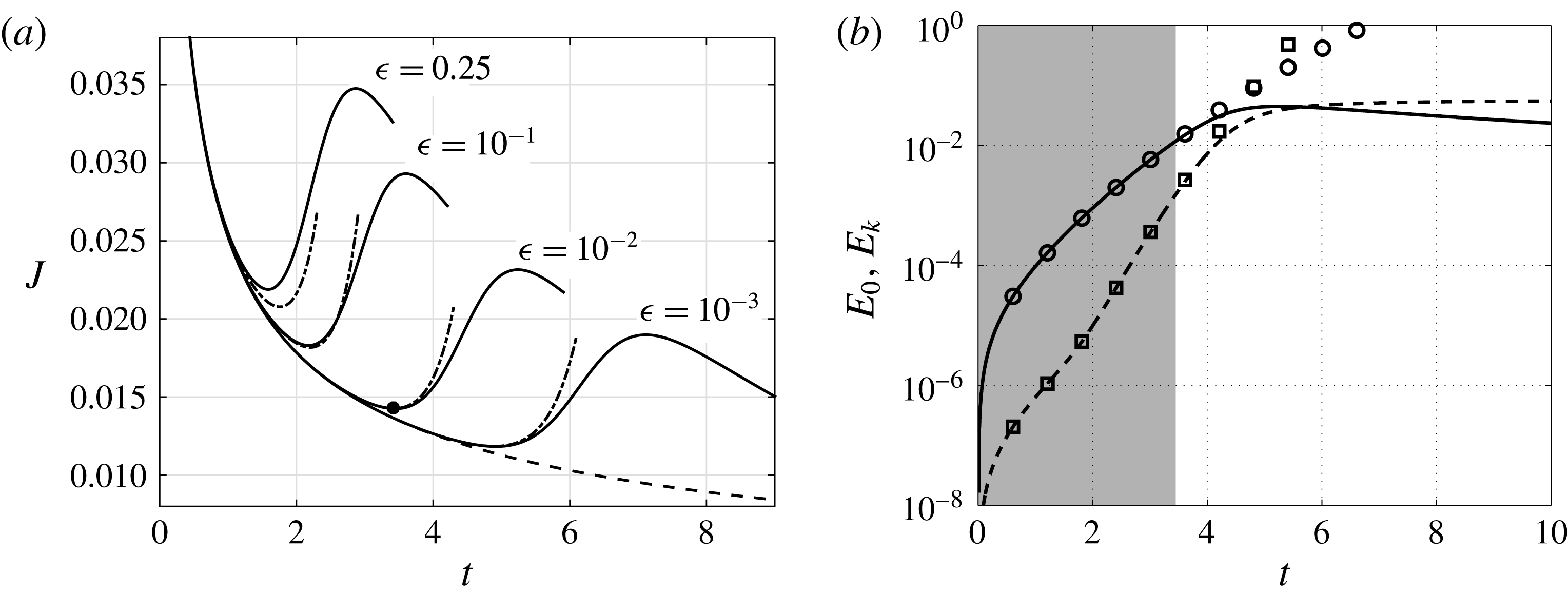
. Figure 2(a) compares DNS (solid lines) and expansion (dash-dotted lines) results for the flux
 $J$
when the system is perturbed with the horizontal wavelength
 $k=30$
and magnitudes
 $\unicode[STIX]{x1D716}=0.25$
,
 $10^{-1}$
,
 $10^{-2}$
and
 $10^{-3}$
. The dashed line shows the flux
 $J_{b}$
produced by the base state. After an initial linear regime, during which
 $J$
decreases, nonlinear mechanisms cause
 $J$
to undergo a turning point and begin increasing. We define this turning point as the onset time of nonlinear convection
 $t_{on}$
. The solid dot shows the DNS result for
 $t_{on}$
when
 $\unicode[STIX]{x1D716}=10^{-2}$
. For
 $\unicode[STIX]{x1D716}\leqslant 10^{-1}$
, the expansion accurately predicts the
 $t_{on}$
measured by DNS, after which the expansion breaks down due to secular terms (see discussion in Nayfeh Reference Nayfeh1981; Tilton & Riaz Reference Tilton and Riaz2014). For example, for
 $\unicode[STIX]{x1D716}=10^{-2}$
, the expansion predicts
 $t_{on}=3.427$
, compared to the DNS result of
 $t_{on}=3.446$
, a relative difference below 1 %. For
 $\unicode[STIX]{x1D716}=0.25$
, however, the expansion predicts a significantly later onset time than the DNS. This is not unexpected, as
 $\unicode[STIX]{x1D716}=0.25$
violates our assumption that
 $\unicode[STIX]{x1D716}\ll 1$
. It suggests, however, that our approach fails for aquifers with significant geologic heterogeneities. For recent work on such systems, we refer to Agartan et al. (Reference Agartan, Trevisan, Cihan, Birkholzer, Zhou and Illangasekare2015). Although we see good agreement up to
 $\unicode[STIX]{x1D716}=10^{-1},$
we restrict our following analysis to
 $\unicode[STIX]{x1D716}\leqslant 10^{-2}.$
Results when
 $Ra=500$
,
 $k=30$
,
 $\unicode[STIX]{x1D706}_{z}=1$
and
 $\unicode[STIX]{x1D6FD}=0$
. (a) DNS (solid lines) and expansion (dash-dotted lines) results for
 $J$
when
 $\unicode[STIX]{x1D716}=0.25$
,
 $10^{-1}$
,
 $10^{-2}$
and
 $10^{-3}$
. The dashed line shows the flux
 $J_{b}$
due to
 $c_{b}$
. The solid dot shows the DNS result for
 $t_{on}$
when
 $\unicode[STIX]{x1D716}=10^{-2}$
. (b) DNS results for
 $E_{k}$
(solid line) and
 $E_{0}$
(dashed line) when
 $\unicode[STIX]{x1D716}=10^{-2}$
. The linear regime
 $t\leqslant t_{on}$
is shaded grey. Expansion results for
 $E_{k}$
(circles) and
 $E_{0}$
(squares) are shown using symbols.

Figure 2(b) shows DNS results for the growth of the fundamental mode,
 $E_{k}$
(solid line) and zero-wavenumber response,
 $E_{0}$
(dashed line) when
 $\unicode[STIX]{x1D716}=10^{-2}$
. The linear regime
 $t\leqslant t_{on}$
is shaded grey. Contrary to previous stability analyses, the perturbation growth is immediate (
 $t_{c}=0$
). This is not surprising, and can be traced to the first-order stability problem (3.4)–(3.5) in which the non-zero forcing
 $F_{1}$
causes an immediate deviation of
 $c_{1}$
from its initial zero value. We observed similar behaviour for all simulations considered in the current study, except in special cases described as ‘mode switching’ in § 4.2. This demonstrates that onset of convection can occur without a finite critical time
 $t_{c}$
, and brings into question the considerable literature focused on characterizing onset of convection using
 $t_{c}$
(for review, see Tilton et al.
Reference Tilton, Daniel and Riaz2013).
Figure 2(b) shows that after the initial linear regime, there is a subsequent nonlinear regime during which the DNS results for
 $E_{0}$
and
 $E_{k}$
attain maxima, and the zero-wavenumber magnitude
 $E_{0}$
surpasses that of the fundamental. For comparison, figure 2(b) also shows the expansion results for
 $E_{0}$
(squares) and
 $E_{k}$
(circles). As expected, we observe good agreement in the linear shaded regime, followed by breakdown of the expansion in the nonlinear regime. Similar behaviour was observed by Tilton & Riaz (Reference Tilton and Riaz2014).
We repeated the computations shown in figure 2 using a range of initial times between
 $0.001\leqslant t_{0}\leqslant 0.1$
and found that
 $t_{0}$
had a negligible effect on
 $t_{on}$
. This is in contrast to the previous stability analyses that perturb the initial concentration field. With that approach, Daniel et al. (Reference Daniel, Tilton and Riaz2013) and Tilton & Riaz (Reference Tilton and Riaz2014) have shown that the initial perturbation time has a strong effect on
 $t_{on}$
. This suggests that the notion of an optimal initial time may be irrelevant in systems perturbed by the porosity field.
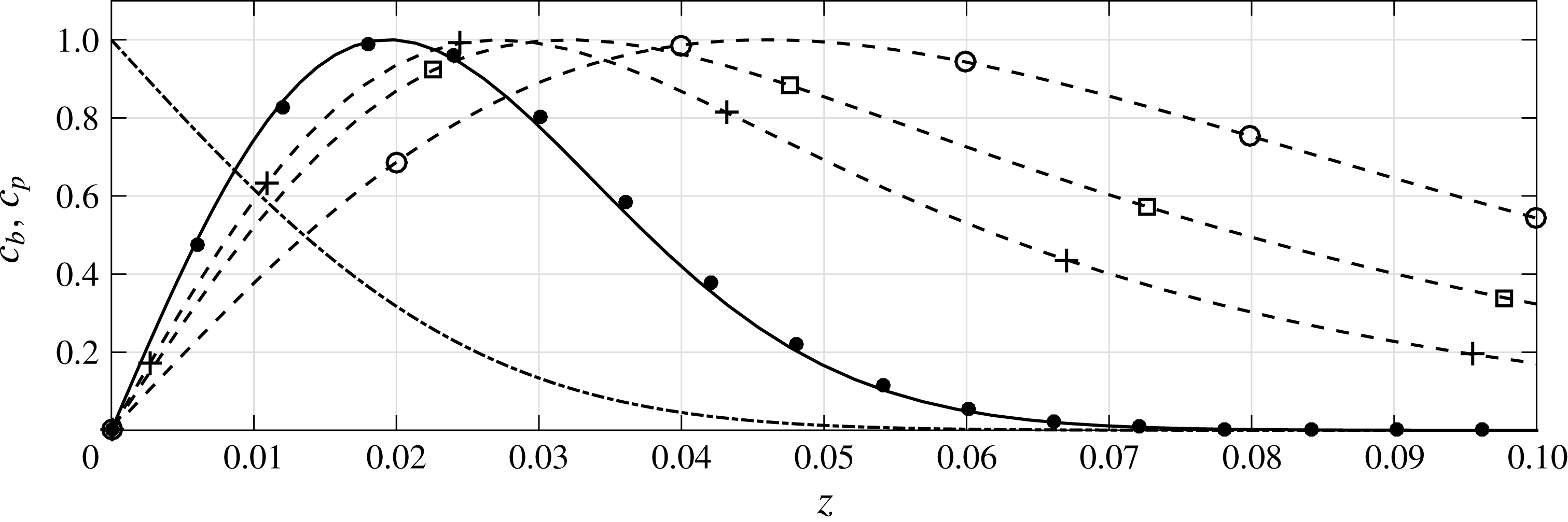
A comparison of the perturbation profiles
 $c_{p}(z,t)$
generated by the current method (solid line), initial condition (4.4) (solid dots), a popular QSM method referred to as QSSA
 $_{z}$
in Tilton et al. (Reference Tilton, Daniel and Riaz2013) (plus signs), the method of Slim & Ramakrishnan (Reference Slim and Ramakrishnan2010) (squares) and the method of Rapaka et al. (Reference Rapaka, Chen, Pawar, Stauffer and Zhang2008) (circles). The profiles are shown at time
 $t=0.1$
for the parameters
 $Ra=500$
and
 $k=30$
. The profile for the current method was generated using
 $\unicode[STIX]{x1D706}_{z}=1$
, and
 $\unicode[STIX]{x1D6FD}=0$
. All parameters for the other methods can be found in figure 9 of Tilton et al. (Reference Tilton, Daniel and Riaz2013).

Previous analyses have generated considerable discussion concerning the physical relevance of predicted concentration perturbation structures (Riaz et al. Reference Riaz, Hesse, Tchelepi and Orr2006; Daniel et al. Reference Daniel, Tilton and Riaz2013; Tilton et al. Reference Tilton, Daniel and Riaz2013). The debate arises due to the fact that QSM and IVP methods can produce perturbation structures for which the sum of the base state and perturbation produces unphysical negative concentrations. To judge the relevance of such perturbations, Tilton et al. (Reference Tilton, Daniel and Riaz2013) defined a net concentration field
 $$\begin{eqnarray}c_{net}(x,z,t)=c_{b}(z,t)+A_{\infty }\cos (kx)c_{p}(z,t),\end{eqnarray}$$
where
 $c_{p}(z,t)$
is the concentration perturbation profile at time
 $t$
normalized so its peak value is unity, and
 $A_{\infty }=\Vert c_{net}-c_{b}\Vert _{\infty }$
is the perturbation magnitude. For every perturbation, there is a maximum allowable magnitude
 $A_{max}$
beyond which
 $c_{net}$
produces unphysical negative concentrations. If
 $A_{max}$
tends to zero, the perturbation cannot support finite magnitudes, which implies it cannot exist in physical systems.
In the current study, we find that perturbations to the concentration field arise naturally without producing negative concentrations. In contrast to other methods, the perturbation structures do not need to be verified a posteriori to judge their physical relevance. The solid line in figure 3 shows the expansion result for
 $c_{p}$
at time
 $t=0.1$
when the system is perturbed using
 $k=30$
. The base state
 $c_{b}(z,t)$
is shown as a dashed-dotted line. For comparison, the solid dots show the result produced using a popular initial concentration perturbation proposed by Riaz et al. (Reference Riaz, Hesse, Tchelepi and Orr2006),
 $$\begin{eqnarray}c_{p}=\unicode[STIX]{x1D709}\text{e}^{-\unicode[STIX]{x1D709}^{2}},\quad \unicode[STIX]{x1D709}=z\sqrt{Ra/(4t)}.\end{eqnarray}$$
We see close agreement between (4.4) and the structures produced with the current method. Although not shown for brevity, we also find qualitative agreement with the non-modal analysis of Daniel et al. (Reference Daniel, Tilton and Riaz2013). Figure 3 demonstrates, however, that we find poor agreement with a popular QSM method referred to as QSSA
 $_{z}$
in Tilton et al. (Reference Tilton, Daniel and Riaz2013) (plus signs) and the optimization methods of Slim & Ramakrishnan (Reference Slim and Ramakrishnan2010) (squares) and Rapaka et al. (Reference Rapaka, Chen, Pawar, Stauffer and Zhang2008) (circles). As discussed in Tilton et al. (Reference Tilton, Daniel and Riaz2013), these methods produce perturbations that have a similar spatial structure to the current study, but they extend beyond the transient diffusive base state such that they cannot support finite values of
 $A_{max}$
.
For a fixed Rayleigh number,
 $Ra$
, wavenumber
 $k$
and shape function
 $f(z)$
, expansion (3.1) only needs to be solved once, after which
 $\unicode[STIX]{x1D716}$
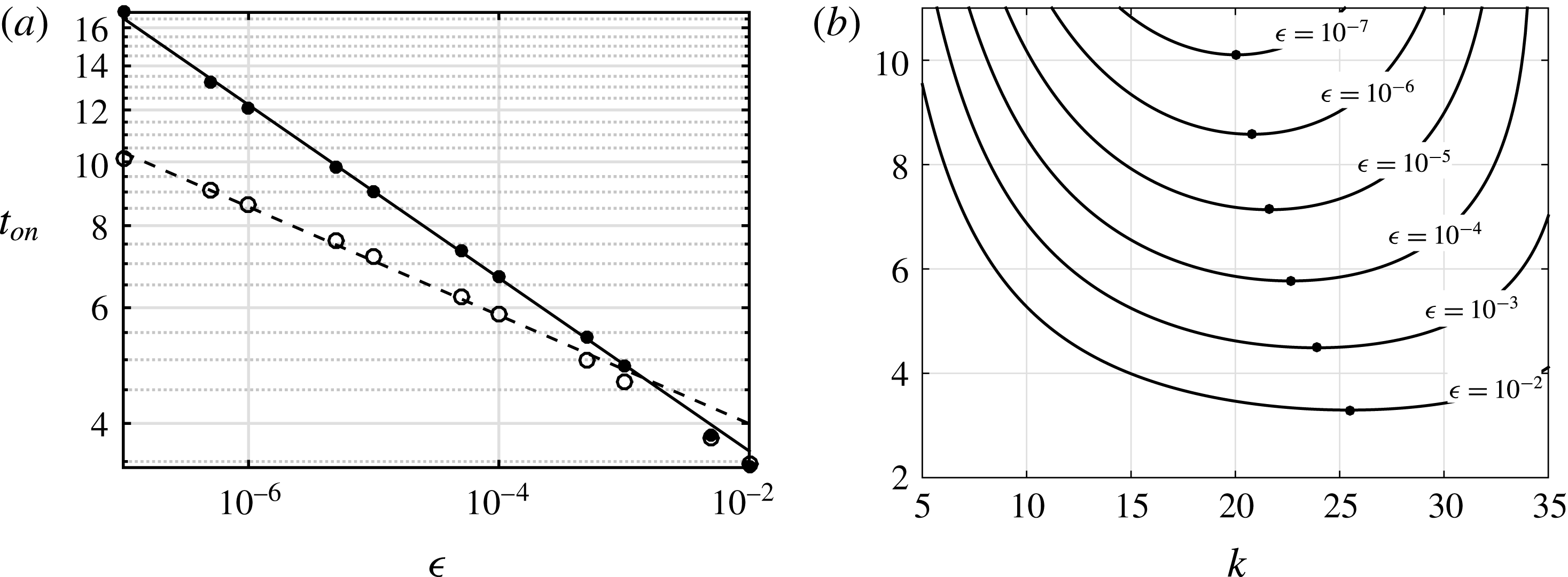
can be varied independently. This procedure was used to generate figure 4(a) showing the variation of
 $t_{on}$
with
 $\unicode[STIX]{x1D716}$
for the fixed wavenumbers
 $k=30$
(solid dots) and
 $k=20$
(open circles). We observe that for a fixed wavenumber,
 $t_{on}$
tends to a power-law relationship for sufficiently small
 $\unicode[STIX]{x1D716}$
. The lines show the best fits
 $t_{on}=1.97\unicode[STIX]{x1D716}^{-0.132}$
(solid line) and
 $t_{on}=2.64\unicode[STIX]{x1D716}^{-0.0850}$
(dashed line), demonstrating that the exponent in the power law varies with
 $k$
.
Expansion results for
 $t_{on}$
when
 $Ra=500$
,
 $\unicode[STIX]{x1D706}_{z}=1$
and
 $\unicode[STIX]{x1D6FD}=0$
. (a)
 $t_{on}$
versus perturbation magnitude
 $\unicode[STIX]{x1D716}$
when
 $k=30$
(solid dots) and
 $k=20$
(open circles). The lines show the best fits
 $t_{on}=1.97\unicode[STIX]{x1D716}^{-0.132}$
(solid line) and
 $t_{on}=2.64\unicode[STIX]{x1D716}^{-0.0850}$
(dashed line). (b)
 $t_{on}$
as a function of wavenumber
 $k$
and magnitude
 $\unicode[STIX]{x1D716}$
. Solid dots mark (
 $k_{on}^{min}$
,
 $t_{on}^{min}$
).

The curves in figure 4(b) show the variation of
 $t_{on}$
with
 $k$
and
 $\unicode[STIX]{x1D716}$
. The curves were generated by solving expansion (3.1) for wavenumbers
 $5\leqslant k\leqslant 35$
in increments of 0.1. The solid dots in figure 4(b) demonstrate that for a given perturbation magnitude,
 $\unicode[STIX]{x1D716}$
, there is a wavenumber
 $k_{on}^{min}$
that minimizes the onset time for nonlinear convection. The minimum onset time,
 $t_{on}^{min}$
, decreases with perturbation magnitude, while
 $k_{on}^{min}$
increases with perturbation magnitude. In contrast to
 $t_{on}$
in figure 4(a), however, we find that
 $t_{on}^{min}$
and
 $k_{on}^{min}$
do not satisfy simple power-law relationships. The following quadratic fits in terms of
 $\log _{10}\unicode[STIX]{x1D716}$
provide errors of the order of
 $0.01$
% in comparison with the expansion results,
 $$\begin{eqnarray}\displaystyle & \displaystyle t_{on}^{min}\approx 0.04117(\log _{10}\unicode[STIX]{x1D716})^{2}-0.9921\log _{10}\unicode[STIX]{x1D716}+1.144, & \displaystyle\end{eqnarray}$$
 $$\begin{eqnarray}\displaystyle & \displaystyle k_{on}^{min}\approx 0.1032(\log _{10}\unicode[STIX]{x1D716})^{2}+1.987\log _{10}\unicode[STIX]{x1D716}+28.96. & \displaystyle\end{eqnarray}$$
The results for
 $t_{on}$
in figure 4 are qualitatively similar to those produced using IVP methods that introduce an initial concentration perturbation. In that case, Tilton et al. (Reference Tilton, Daniel and Riaz2013) showed that for fixed
 $k$
, the onset time
 $t_{on}$
satisfies power-law relationships in terms of the initial concentration perturbation magnitude. Subsequently, Tilton & Riaz (Reference Tilton and Riaz2014) demonstrated the existence of
 $(k_{on}^{min},t_{on}^{min})$
. As here, the authors found that
 $(k_{on}^{min},t_{on}^{min})$
did not satisfy power laws. This likely occurs due to the variation of the exponents in the power laws, as demonstrated in figure 4(a).
The onset conditions
 $(k_{on}^{min},t_{on}^{min})$
observed in the current study are of comparable magnitude to those produced by the IVP approach of Tilton & Riaz (Reference Tilton and Riaz2014). Consequently, although the current method produces zero critical times for linear instability,
 $t_{c}=0$
, it does not produce smaller onset times
 $t_{on}$
than previous analyses. The major advantage of the current approach is that it focuses attention on
 $t_{on}$
, and removes long-standing debate concerning
 $t_{c}$
,
 $t_{p}$
, and non-physical perturbation structures. Moreover, while it is not clear that initial concentration perturbations can be measured or controlled in porous media, the spatial variation of porosity can be estimated using well logs (Delfiner Reference Delfiner2007). The spatial variation of porosity can also be controlled experimentally (Agartan et al.
Reference Agartan, Trevisan, Cihan, Birkholzer, Zhou and Illangasekare2015). However, we see that even small porosity perturbations of the order of
 $\unicode[STIX]{x1D716}\sim 10^{-7}$
are sufficient to trigger convection at onset times comparable to previous studies. This observation is significant, because studies of convection in heterogeneous media often ignore porosity variations by arguing that their influence is small (De Wit & Homsy Reference De Wit and Homsy1997; Daniel et al.
Reference Daniel, Riaz and Tchelepi2015).
A final note is warranted for the case of zero horizontal wavenumber,
 $k=0$
. For this case, equations (3.12) produce the trivial solution
 $\boldsymbol{v}=0$
. This removes all convective effects from the first and second-order problems such that nonlinear convection cannot occur. Nevertheless, our DNS shows a small deviation of
 $J$
from
 $J_{b}$
due to the remaining dispersion effects. In contrast to nonlinear convection, however, the deviation is such that
 $J$
can be less than
 $J_{b}$
. As in all previous QSM and IVP analyses, we conclude that instability requires a non-zero horizontal wavenumber (
 $k\neq 0$
) to trigger convection.
4.2 Effects of vertical wavenumber
$\unicode[STIX]{x1D706}_{z}$
and phase shift
$\unicode[STIX]{x1D6FD}$


The efficiency of our expansion allows us to perform a parametric study of the effects of
 $\unicode[STIX]{x1D716}$
,
 $k$
,
 $\unicode[STIX]{x1D706}_{z}$
,
 $\unicode[STIX]{x1D6FD}$
and
 $Ra$
on the onset time of nonlinear convection. We begin by exploring the effects of the vertical wavenumber
 $\unicode[STIX]{x1D706}_{z}$
by setting
 $\unicode[STIX]{x1D6FD}=0$
so as to consider perturbations of the form
 $\widetilde{\unicode[STIX]{x1D719}}(x,z)=\cos (kx)\cos (2\unicode[STIX]{x03C0}z/\unicode[STIX]{x1D706}_{z})$
. We then find the optimal combinations of horizontal and vertical wavelength (
 $k_{on}^{opt}$
,
 $\unicode[STIX]{x1D706}_{z}^{opt}$
) that minimize the onset time of nonlinear convection (
 $t_{on}^{opt}$
). In practice, this was done by computing
 $(k_{on}^{min},t_{on}^{min})$
, as demonstrated in figure 4(b), for horizontal wavelengths
 $1\leqslant k\leqslant 30$
, vertical wavelengths
 $0.01\leqslant \unicode[STIX]{x1D706}_{z}\leqslant 1$
and perturbation magnitudes
 $10^{-2}\leqslant \unicode[STIX]{x1D716}\leqslant 10^{-7}$
.
Effect of vertical wavenumber
 $\unicode[STIX]{x1D706}_{z}$
on expansion results when
 $Ra=500$
and
 $\unicode[STIX]{x1D6FD}=0$
. (a) Variation of
 $t_{on}^{min}$
(solid line, left axis) and
 $k_{on}^{min}$
(dashed line, right axis) with varying
 $\unicode[STIX]{x1D706}_{z}$
for fixed
 $\unicode[STIX]{x1D716}=10^{-7}$
. The circle symbols mark
 $t_{on}^{opt}$
and
 $k_{on}^{opt}$
. (b) The variation of
 $t_{on}^{opt}$
(solid line with circles) and
 $k_{on}^{opt}$
(solid line with squares) as a function of perturbation magnitude
 $\unicode[STIX]{x1D716}$
. The dashed lines show the corresponding results when
 $\unicode[STIX]{x1D6FD}=0.25$
.

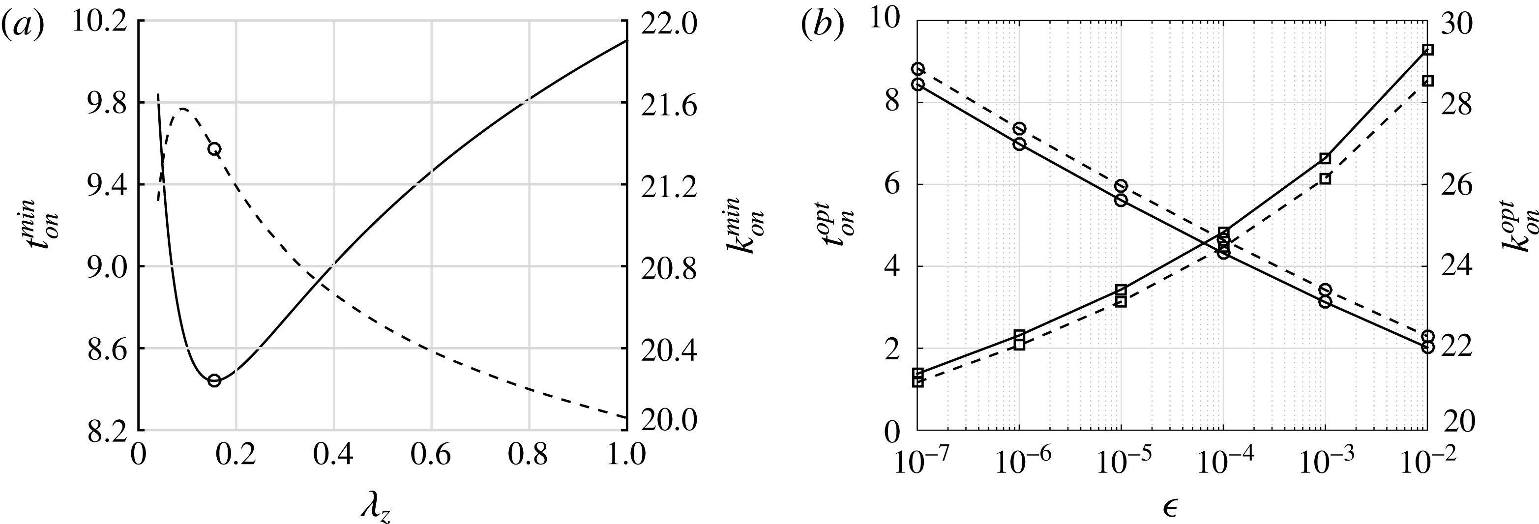
Figure 5(a) shows the resulting variation of
 $t_{on}^{min}$
(solid line, left axis) and
 $k_{on}^{min}$
(dashed line, right axis) with varying
 $\unicode[STIX]{x1D706}_{z}$
for fixed
 $\unicode[STIX]{x1D716}=10^{-7}$
. We see that
 $t_{on}^{min}$
reaches a minimum value
 $t_{on}^{opt}=8.441$
(circular symbol) at the vertical wavelength
 $\unicode[STIX]{x1D706}_{z}^{opt}=0.154$
for which the horizontal wavenumber is
 $k_{on}^{opt}=21.4$
(circular symbol). Figure 5(b) shows the resulting variation of
 $t_{on}^{opt}$
(solid line with circles) and
 $k_{on}^{opt}$
(solid line with squares) as a function of
 $\unicode[STIX]{x1D716}$
. The following best fits agree with the expansion results to within 0.5 %
 $$\begin{eqnarray}\displaystyle & \displaystyle t_{on}^{opt}=0.04402(\log _{10}\unicode[STIX]{x1D716})^{2}-0.8894\log _{10}\unicode[STIX]{x1D716}+0.0601, & \displaystyle\end{eqnarray}$$
 $$\begin{eqnarray}\displaystyle & \displaystyle k_{on}^{opt}=0.2023(\log _{10}\unicode[STIX]{x1D716})^{2}+3.363\log _{10}\unicode[STIX]{x1D716}+35.10, & \displaystyle\end{eqnarray}$$
 $$\begin{eqnarray}\displaystyle & \displaystyle \unicode[STIX]{x1D706}_{z}^{opt}=0.1360\unicode[STIX]{x1D716}^{-0.008074}. & \displaystyle\end{eqnarray}$$
The non-monotonic variation of
 $t_{on}^{min}$
with
 $\unicode[STIX]{x1D706}_{z}$
in figure 5(a) suggests a resonant interaction between the porosity perturbation and an intrinsic length scale for the buoyancy-driven instability. Similar resonance has been observed in studies of viscous fingering (De Wit & Homsy Reference De Wit and Homsy1997) and transient convection (Daniel et al.
Reference Daniel, Riaz and Tchelepi2015) in spatially periodic permeability fields. Those studies investigated resonance using quasi-steady linear modal analyses in which the permeability field and flow fields were independently perturbed so that interactions between their wavenumbers could be investigated. As this follows a philosophically different QSM approach to the current, we leave such analysis to future consideration. Rather, we interpret the potential resonance by considering the length scales characterizing onset of nonlinear convection.
From relations (4.8)–(4.9), we observe that the optimal vertical wavelength decreases from
 $\unicode[STIX]{x1D706}_{z}^{opt}=0.154$
for
 $\unicode[STIX]{x1D716}=10^{-7}$
to
 $\unicode[STIX]{x1D706}_{z}^{opt}=0.141$
for
 $\unicode[STIX]{x1D716}=10^{-2}$
. Similarly, the optimal horizontal wavelength,
 $\unicode[STIX]{x1D706}_{x}^{opt}=2\unicode[STIX]{x03C0}/k_{on}^{opt}$
, decreases from
 $\unicode[STIX]{x1D706}_{x}^{opt}=0.294$
to
 $\unicode[STIX]{x1D706}_{x}^{opt}=0.215$
. These length scales may be compared with the depth of the transient diffusive base state,
 $c_{b}(z,t)$
. For the time scales considered here, we can approximate the boundary layer depth were
 $c_{b}\approx 0.005$
as
 $\unicode[STIX]{x1D6FF}(t)=4\sqrt{t/Ra}$
. We find that the boundary layer depth at
 $t_{on}^{opt}$
varies from
 $\unicode[STIX]{x1D6FF}^{opt}=0.52$
for
 $\unicode[STIX]{x1D716}=10^{-7}$
to
 $\unicode[STIX]{x1D6FF}^{opt}=0.254$
for
 $\unicode[STIX]{x1D716}=10^{-2}$
. We conclude that
 $\unicode[STIX]{x1D706}_{z}^{opt}$
,
 $\unicode[STIX]{x1D706}_{x}^{opt}$
and
 $\unicode[STIX]{x1D6FF}^{opt}$
are of equal order. Similar length scales have been observed in stability analyses that initiate instability using an initial concentration perturbation. For example, comparing figure 4(b) of the current study with figure 2(b) of Tilton & Riaz (Reference Tilton and Riaz2014), we see that the current approach produces optimal horizontal wavenumbers of comparable magnitude to those of Tilton & Riaz (Reference Tilton and Riaz2014).
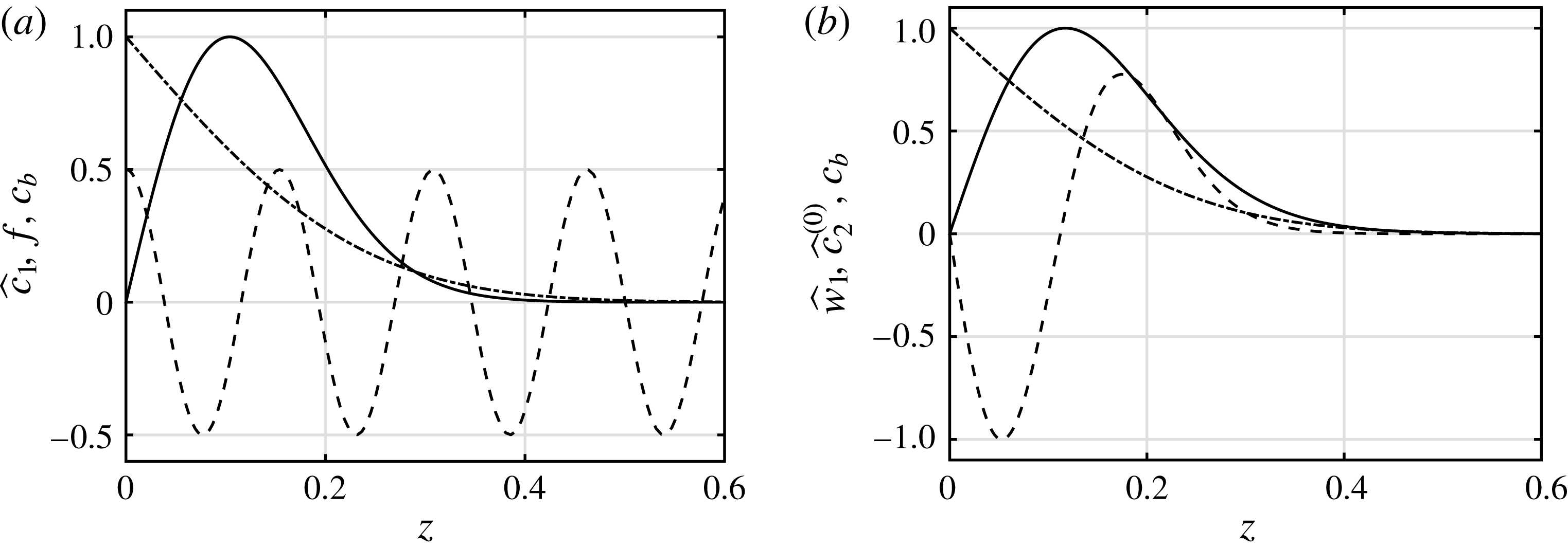
Figure 6(a) compares the porosity perturbation profile
 $f(z)$
with the first-order concentration perturbation
 $\widehat{c}_{1}(z,t)$
and the base state
 $c_{b}(z,t)$
for the optimal state
 $(\unicode[STIX]{x1D706}_{z}^{opt},k_{on}^{opt},t_{on}^{opt})$
labelled with circular symbols in figure 5(a). Panel (b) Shows the corresponding profiles of the first-order velocity perturbation
 $\widehat{w}_{1}(z,t)$
and the zero-wavenumber response
 $\widehat{c}_{2}^{(0)}(z,t)$
. Although not shown for brevity, we observe that the profiles
 $\widehat{c}_{1}$
,
 $\widehat{w}_{1}$
and
 $\widehat{c}_{2}^{(0)}$
shown in figure 6 vary little with changes in
 $\unicode[STIX]{x1D706}_{z}$
, and are always of comparable depth to the base state. This suggests that the flow field perturbation profiles are primarily determined by
 $c_{b}$
, and that
 $\unicode[STIX]{x1D706}_{z}^{opt}$
is that for which
 $f(z)$
also varies over a distance comparable to
 $c_{b}$
. The result that
 $\unicode[STIX]{x1D706}_{z}^{opt}$
is consistently smaller than
 $\unicode[STIX]{x1D6FF}^{opt}$
can be partially explained by noting that the boundary layer depth
 $\unicode[STIX]{x1D6FF}(t)$
increases with time, from
 $\unicode[STIX]{x1D6FF}=0$
at
 $t=0$
to
 $\unicode[STIX]{x1D6FF}=\unicode[STIX]{x1D6FF}^{opt}$
at
 $t=t_{on}^{opt}$
. Consequently,
 $\unicode[STIX]{x1D706}_{z}^{opt}$
likely corresponds to an intermediate value that maximizes the net perturbation growth over the linear regime.
Perturbation profiles in the vertical
 $z$
-direction for the optimal parameters
 $(\unicode[STIX]{x1D706}_{z}^{opt},k_{on}^{opt},t_{on}^{opt})=(0.154,21.4,8.441)$
denoted by the open circular symbols in figure 5(a). (a) Comparison of
 $\widehat{c}_{1}(z,t)$
(solid line),
 $f(z,t)$
(dashed line) and
 $c_{b}$
(dash-dotted line). (b) Comparison of
 $\widehat{w}_{1}(z,t)$
(solid line),
 $\widehat{c}_{2}^{(0)}$
(dashed line) and
 $c_{b}$
(dash-dotted line). For ease of visualization,
 $\widehat{c}_{1}$
are normalized with respect to their absolute peak values.

Effect of vertical wavenumber
 $\unicode[STIX]{x1D706}_{z}$
on expansion results when
 $Ra=500$
and
 $\unicode[STIX]{x1D6FD}=0.25$
. (a) Variation of
 $t_{on}^{min}$
(solid line, left axis) and
 $k_{on}^{min}$
(dashed line, right axis) with varying
 $\unicode[STIX]{x1D706}_{z}$
for fixed
 $\unicode[STIX]{x1D716}=10^{-7}$
. The symbols mark
 $t_{on}^{opt}$
(circle) and
 $k_{on}^{opt}$
(square). (b) Expansion results for
 $t_{on}$
as a function of wavenumber
 $k$
and perturbation magnitude
 $\unicode[STIX]{x1D716}$
when
 $\unicode[STIX]{x1D706}_{z}=0.16$
. Solid dots mark (
 $k_{on}^{min}$
,
 $t_{on}^{min}$
).

To investigate the effects of the vertical offset, we repeat our above analysis for
 $\unicode[STIX]{x1D6FD}=0.25$
, which corresponds to a perturbation of the form
 $\widetilde{\unicode[STIX]{x1D719}}(x,z)=\cos (kx)\sin (2\unicode[STIX]{x03C0}z/\unicode[STIX]{x1D706}_{z}).$
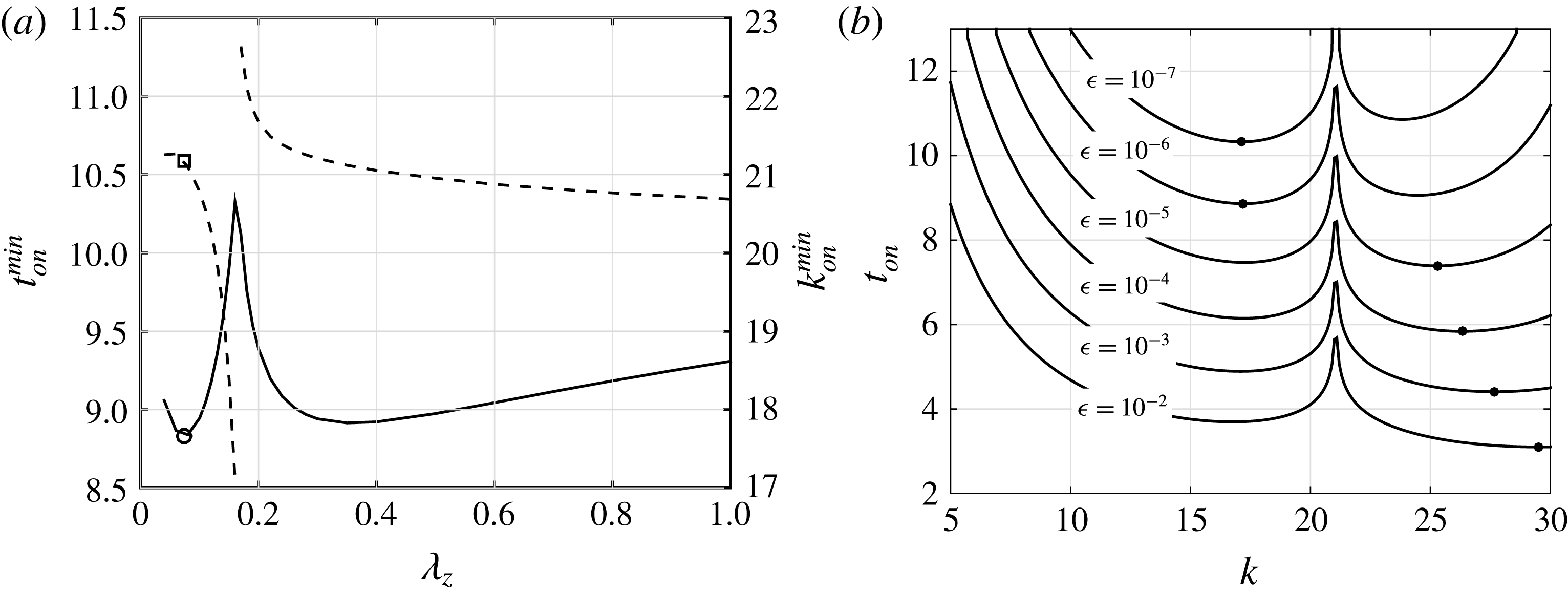
Figure 7(a) shows the resulting variation of
 $t_{on}^{min}$
(solid line, left axis) and
 $k_{on}^{min}$
(dashed line, right axis) with varying
 $\unicode[STIX]{x1D706}_{z}$
for
 $\unicode[STIX]{x1D716}=10^{-7}$
. We observe that the variations of
 $t_{on}^{min}$
and
 $k_{on}^{min}$
are more complicated than those shown earlier for
 $\unicode[STIX]{x1D6FD}=0$
in figure 5(a). Most notably, near
 $\unicode[STIX]{x1D706}_{z}=0.16$
, there is a discontinuity in
 $k_{on}^{min}$
and a local maximum in
 $t_{on}^{min}$
. This behaviour arises due to a fold that forms in the
 $t_{on}$
versus
 $k$
curve. This is demonstrated in figure 7(b) showing
 $t_{on}$
versus
 $k$
for
 $\unicode[STIX]{x1D706}_{z}=0.16$
and
 $10^{-7}\leqslant \unicode[STIX]{x1D716}\leqslant 10^{-2}$
. We see that the formation of a fold centred about
 $k=21.051$
causes a sudden increase in
 $k_{on}^{min}$
with increasing
 $\unicode[STIX]{x1D716}$
. For
 $\unicode[STIX]{x1D6FD}=0.25$
, such folds were only observed for vertical wavelengths between roughly
 $0.15\leqslant \unicode[STIX]{x1D706}_{z}\leqslant 0.20$
. No such folds were observed for
 $\unicode[STIX]{x1D6FD}=0$
.
The dashed lines in figure 5(b) show
 $t_{on}^{opt}$
(circles) and
 $k_{on}^{opt}$
(solid line) as a function of
 $\unicode[STIX]{x1D716}$
when
 $\unicode[STIX]{x1D6FD}=0.25$
. Despite the formation of the above-mentioned fold, the variation of (
 $k_{on}^{opt}$
,
 $t_{on}^{opt}$
) remains smooth, and varies only little from the results for
 $\unicode[STIX]{x1D6FD}=0.$
The following best fits agree with the expansion results to within 0.5 %
 $$\begin{eqnarray}\displaystyle & \displaystyle t_{on}^{opt}=0.04368(\log _{10}\unicode[STIX]{x1D716})^{2}-0.9156\log _{10}\unicode[STIX]{x1D716}+0.2860, & \displaystyle\end{eqnarray}$$
 $$\begin{eqnarray}\displaystyle & \displaystyle k_{on}^{opt}=0.1765(\log _{10}\unicode[STIX]{x1D716})^{2}+3.028\log _{10}\unicode[STIX]{x1D716}+33.79, & \displaystyle\end{eqnarray}$$
 $$\begin{eqnarray}\displaystyle & \displaystyle \unicode[STIX]{x1D706}_{z}^{opt}=0.06474\unicode[STIX]{x1D716}^{-0.008304}. & \displaystyle\end{eqnarray}$$
We observe from figure 5(b) that the optimal perturbations with
 $\unicode[STIX]{x1D6FD}=0.25$
produce later onset times than for
 $\unicode[STIX]{x1D6FD}=0$
(solid lines). From (4.12), we see that they also have smaller optimal vertical wavelengths, varying from
 $\unicode[STIX]{x1D706}_{z}^{opt}=0.0736$
for
 $\unicode[STIX]{x1D716}=10^{-7}$
to
 $\unicode[STIX]{x1D706}_{z}^{opt}=0.0669$
for
 $\unicode[STIX]{x1D716}=10^{-2}$
. We repeated our analysis above for
 $\unicode[STIX]{x1D6FD}=0.125$
and
 $0.375$
and found that of the four offset’s considered (
 $\unicode[STIX]{x1D6FD}=0,$
0.125, 0.25 and 0.375),
 $\unicode[STIX]{x1D6FD}=0$
produced the earliest onset times, while
 $\unicode[STIX]{x1D6FD}=0.25$
produced the latest onset times. Consequently, relations (4.7) and (4.10) provide upper and lower bounds on time
 $t_{on}^{opt}$
.
The folds in figure 7(b) suggest a potential mode switching in the underlying instability. Indeed, mode switching has been observed in systems with heterogeneous permeability (Daniel et al.
Reference Daniel, Riaz and Tchelepi2015). In that case, switching occurs due to an additional vorticity generation mechanism introduced in the right-hand side of the vorticity equation (3.7). In the current study, however, the source is less clear. If we consider (3.11), which governs the evolution of
 $\widehat{c}_{1}$
, we note that the forcing term
 $(1/Ra)(\text{d}f/\text{d}z)(\unicode[STIX]{x2202}c_{b}/\unicode[STIX]{x2202}z)$
is independent of
 $k$
, and consequently cannot explain the formation of folds on its own. This suggests the folds may occur from a competition between the forcing term and the convective term
 $w_{1}(\unicode[STIX]{x2202}c_{b}/\unicode[STIX]{x2202}z)$
on the left-hand side of (3.11). The convective term does depend on
 $k$
, such that particular values of
 $k$
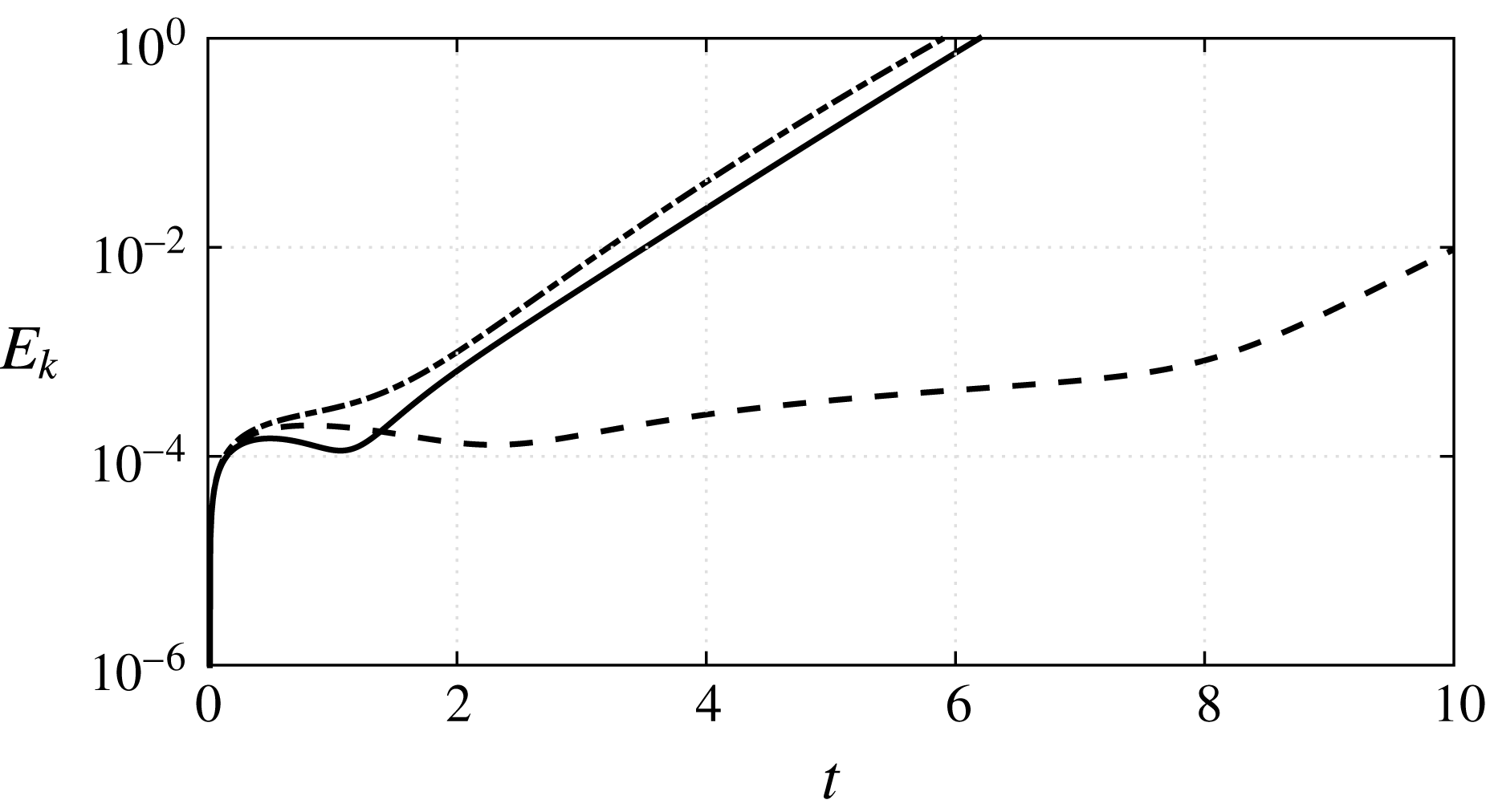
may cause the sum of the convective and forcing terms to delay perturbation growth. This is supported by figure 8 showing the temporal evolution of the perturbation magnitude,
 $E_{k}$
, when
 $k=15$
(solid line),
 $k=21.051$
(dashed line) and
 $k=25$
(dash-dotted line), and all other parameters are as in figure 7(b), i.e.
 $Ra=500$
,
 $\unicode[STIX]{x1D6FD}=0.25$
,
 $\unicode[STIX]{x1D706}_{z}=0.16$
and
 $\unicode[STIX]{x1D716}=10^{-2}$
. We see that in the vicinity of the fold, perturbation growth is delayed and non-monotonic.
4.3 Effects of Rayleigh number,
$Ra$

Although not shown for brevity, we found that for
 $Ra=500$
, the end effects at
 $z=H$
play no role in the onset of nonlinear convection. With increasing
 $Ra$
, onset of nonlinear convection happens at earlier times, so that this conclusion remains valid. Consequently, the Rayleigh number dependence of our results can be removed by re-non-dimensionalizing our problem with respect to the length scale
 $L=\langle \unicode[STIX]{x1D719}\rangle {\mathcal{D}}/U$
and time scale
 $T=\langle \unicode[STIX]{x1D719}\rangle L/U$
. By re-scaling (4.13)–(4.15), we find the following relationships for the optimal perturbations when
 $\unicode[STIX]{x1D6FD}=0$
,
 $$\begin{eqnarray}\displaystyle & \displaystyle \frac{t^{\ast }U^{2}}{\langle \unicode[STIX]{x1D719}\rangle ^{2}{\mathcal{D}}}=t_{on}^{opt}Ra=22.01(\log _{10}\unicode[STIX]{x1D716})^{2}-444.7\log _{10}\unicode[STIX]{x1D716}+30.05, & \displaystyle\end{eqnarray}$$
 $$\begin{eqnarray}\displaystyle & \displaystyle \frac{k^{\ast }\langle \unicode[STIX]{x1D719}\rangle {\mathcal{D}}}{U}=\frac{k_{on}^{opt}}{Ra}=4.046\times 10^{-4}(\log _{10}\unicode[STIX]{x1D716})^{2}+0.006726\log _{10}\unicode[STIX]{x1D716}+0.0702, & \displaystyle\end{eqnarray}$$
 $$\begin{eqnarray}\displaystyle & \displaystyle \frac{\unicode[STIX]{x1D706}_{z}^{\ast }U}{\langle \unicode[STIX]{x1D719}\rangle {\mathcal{D}}}=\unicode[STIX]{x1D706}_{z}^{opt}Ra=68.0\unicode[STIX]{x1D716}^{-0.008074}. & \displaystyle\end{eqnarray}$$
In these equations,
 $t^{\ast }$
,
 $k^{\ast }$
and
 $\unicode[STIX]{x1D706}_{z}^{\ast }$
are the dimensional onset time, horizontal wavenumber and vertical wavenumber of the optimal perturbations, while
 $t_{on}^{opt}$
,
 $k_{on}^{opt}$
and
 $\unicode[STIX]{x1D706}_{z}^{opt}$
are the non-dimensional equivalents given in (4.13)–(4.15).
Evolution of the perturbation magnitude
 $E_{k}$
when
 $Ra=500$
,
 $\unicode[STIX]{x1D6FD}=0.25$
,
 $\unicode[STIX]{x1D706}_{z}=0.16$
,
 $\unicode[STIX]{x1D716}=10^{-2}$
and
 $k=15$
(solid line),
 $k=21.051$
(dashed line) and
 $k=25$
(dash-dotted line).

To put these predictions in physical perspective, we consider the following typical sequestration parameters (Ennis-King & Paterson Reference Ennis-King and Paterson2003):
 $\unicode[STIX]{x1D707}=5\times 10^{-4}~\text{Pa}~\text{s}$
,
 $\unicode[STIX]{x1D719}=0.2$
,
 $\unicode[STIX]{x0394}\unicode[STIX]{x1D70C}=10~\text{kg}~\text{m}^{-3}$
,
 $g=9.81~\text{m}~\text{s}^{-2}$
,
 ${\mathcal{D}}=10^{-9}~\text{m}^{2}~\text{s}^{-1}$
and
 $10^{-14}\leqslant K\leqslant 10^{-12}~\text{m}^{2}$
. Using these values for a high-permeability aquifer,
 $K=10^{-12}~\text{m}^{2}$
, relations (4.13)–(4.15) predict that the optimal onset time, horizontal wavenumber and vertical wavenumber vary between
 $t^{\ast }=51~\text{days}$
,
 $\unicode[STIX]{x1D706}_{x}^{\ast }=15~\text{cm}$
, and
 $\unicode[STIX]{x1D706}_{z}^{\ast }=7.9~\text{cm}$
for
 $\unicode[STIX]{x1D716}=10^{-7}$
and
 $t^{\ast }=12~\text{days}$
,
 $\unicode[STIX]{x1D706}_{x}^{\ast }=11~\text{cm}$
and
 $\unicode[STIX]{x1D706}_{z}^{\ast }=7.2~\text{cm}$
for
 $\unicode[STIX]{x1D716}=10^{-2}$
. For a low-permeability aquifer,
 $K=10^{-14}~\text{m}^{2}$
, the parameters vary between
 $t^{\ast }=1400~\text{years}$
,
 $\unicode[STIX]{x1D706}_{x}^{\ast }=15~\text{m}$
and
 $\unicode[STIX]{x1D706}_{z}^{\ast }=7.9~\text{m}$
for
 $\unicode[STIX]{x1D716}=10^{-7}$
and
 $t^{\ast }=330~\text{years}$
,
 $\unicode[STIX]{x1D706}_{x}^{\ast }=11~\text{m}$
and
 $\unicode[STIX]{x1D706}_{z}^{\ast }=7.2~\text{m}$
for
 $\unicode[STIX]{x1D716}=10^{-2}$
. Comparison of these predictions with experiments is unfortunately not straightforward. Although detailed experiments of perturbation growth have been performed (Kneafsey & Pruess Reference Kneafsey and Pruess2010; Slim et al.
Reference Slim, Bandi, Miller and Mahadevan2013; Outeda et al.
Reference Outeda, El Hasi, D’Onofrio and Zalts2014; Vreme et al.
Reference Vreme, Nadal, Pouligny, Jeandet, Liger-Belair and Meunier2016), they typically use Hele-Shaw cells in which the concept of porosity is unclear. Observations also suggest that convection in Hele-Shaw cells is more likely triggered by initial deformations of the CO
 $_{2}$
-brine interface.
5 Conclusions
We proposed a new approach to studying the linear stability and onset of nonlinear convection in transient diffusive boundary layers in porous media. In contrast to most previous stability analyses, the current method allows concentration perturbations to arise naturally in response to continuous forcing from perturbations in the porosity field. With this approach, perturbation growth is immediate and is insensitive to the initial time of integration. This brings into question previous literature that characterizes instability in terms of
 $t_{c}$
and
 $t_{p}$
(Daniel et al.
Reference Daniel, Tilton and Riaz2013; Tilton et al.
Reference Tilton, Daniel and Riaz2013; Tilton & Riaz Reference Tilton and Riaz2014). Furthermore, in contrast to previous methods, the current method always produces physical concentration fields with non-zero concentrations. The perturbation structures are similar those suggested by Ben et al. (Reference Ben, Demekhin and Chang2002), Riaz et al. (Reference Riaz, Hesse, Tchelepi and Orr2006) and Daniel et al. (Reference Daniel, Tilton and Riaz2013), but different from those of Rapaka et al. (Reference Rapaka, Chen, Pawar, Stauffer and Zhang2008) and Slim & Ramakrishnan (Reference Slim and Ramakrishnan2010).
We also showed that the onset time for nonlinear convection,
 $t_{on}$
, can be accurately predicted using a simple asymptotic expansion. Leveraging the computational efficiency of this expansion, we performed a parametric study of
 $t_{on}$
for spatially periodic porosity perturbations, and showed that optimal combinations of wavelengths minimize
 $t_{on}$
. Moreover, even small porosity perturbations of the order of
 $10^{-7}$
are sufficient to produce onset times comparable to those observed in previous studies. This observation is significant, because studies of convection in heterogeneous media often ignore porosity variations by arguing that they are small.
Our results also suggest a potential resonance behaviour between the vertical wavelength of the porosity perturbation and an intrinsic length scale for the buoyancy-driven instability. The length scale appears to be set primarily by the diffusive base state. In special cases, our results also exhibited a potential mode-switching behaviour. While the present study focused on a non-modal IVP approach, future studies could investigate resonance and mode switching further using quasi-steady modal methods, as in De Wit & Homsy (Reference De Wit and Homsy1997) and Daniel et al. (Reference Daniel, Riaz and Tchelepi2015). Moreover, future studies should consider continuous forcing from simultaneously varying permeability and dispersion effects. Finally, the current approach opens future potential to link the results herein with experimental measurements of spatially varying porosity fields, from either laboratory experiments using controlled media or from actual borehole data.
Acknowledgements
The author gratefully acknowledges helpful discussions with Dr A. Riaz from the University of Maryland, College Park, Dr D. Martinand from the University of Aix-Marseille and Dr T. Illangasekare from the Colorado School of Mines. The author also gratefully acknowledges three anonymous reviewers who suggested the resonance and mode-switching behaviours in § 4.2, and who brought the works of Neitzel et al. (Reference Neitzel, Kirkconnell and Little1995), Chen et al. (Reference Chen, Neitzel and Jankowski1987) and De Wit & Homsy (Reference De Wit and Homsy1997) to the author’s attention.