2.1. Experimental set-up

Experiments are carried out in a closed-circuit wind tunnel with a test section with dimensions of 5.5 m long, 1 m high and 0.8 m wide. The non-uniformity of the flow in the test section is approximately 0.1 % and the longitudinal turbulence intensity is less than 0.4 % for the wind speed range involved. Figure 1(a) presents a schematic of the experimental set-up. The test rig includes five major components, the leading edge, trippers, an upstream plate, a curved ramp and a downstream plate. The rig is placed horizontally on the bottom wall of the test section and spans the entire tunnel width. The leading edge is shaped to the NACA0015 aerofoil profile to avoid flow separation. Following Bai et al. (Reference Bai, Zhou, Zhang, Xu, Wang and Antonia2014) and Cheng et al. (Reference Cheng, Qiao, Zhang, Quadrio and Zhou2021), the flow is tripped using one spanwise array of screws, placed at 0.1 m downstream of the leading edge, which acts to perturb incoming flow, accelerating the formation of the fully developed TBL over the upstream plate. Due to the presence of an APG associated with the ramp, the TBL separates from the curved ramp and then reattaches on the downstream plate. The right-handed Cartesian coordinate system is defined such that its origin O is at the midpoint of the upper edge of the ramp and the coordinates x, y and z are along the streamwise, vertical and spanwise directions, respectively. We use U, V and W to represent the instantaneous velocity components in the x, y and z directions, respectively, which can be decomposed as $U=\overline{U}+u$ , $V=\overline{V}+v$ and $W=\overline{W}+w$ , where the overbar denotes time-averaging, and $u$ , $v$ and $w$ are the fluctuating components. Hereinafter, the superscript asterisk ‘∗’ denotes normalisation by the ramp height h and/or the free stream velocity $U _\infty$ , and bracket ‘ $\langle\ \rangle $ ’ denotes phase-averaging based on the period of the pulsed jet. The h and longitudinal length of the curved ramp are 70 and 202 mm, respectively. The ramp consists of two circular arcs with radii of 282 and 141 mm. Readers should refer to Lardeau & Leschziner (Reference Lardeau and Leschziner2011) for more details, such as the mathematical equations of the curves, regarding the curved ramp model. The expansion ratio of the heights downstream of the ramp to that upstream is 1.1, which is sufficiently small to avoid the interference effect of the wind tunnel (Song et al. Reference Song, Degraa and Eaton2000; Zhang & Zhong Reference Zhang and Zhong2010; Lim et al. Reference Lim and Lyu2021). The width-to-height ratio of the ramp is 11.2, larger than the critical value of 10 to ensure the two-dimensionality of the baseline flow (Park et al. Reference Park, Jeon, Choi and Yoo2007; Ma & Schroder Reference Ma and Schröder2017; Li et al. Reference Li, Zhang, Liu, Wu and Gao2020), thus ensuring negligible three-dimensional effects from the side walls of the test section. This is confirmed by the measured spanwise distribution of the time-averaged pressure coefficient ( $\overline{C_{p}}$ ) on the ramp (Stella, Mazellier & Kourta Reference Stella, Mazellier and Kourta2017), which is constant for z ^* = −4 to 4 within experimental uncertainties.

Figure 1(c) shows the pressurised air supply and regulation system. The airflow from the air compressor is filtered and dried through the air filter, and is then stabilised and adjusted in pressure via a high-precision pressure relief valve (SMC IR3020). Ideally, given a fixed supply pressure, the mass flow rate should be independent of the excitation frequency $f_{e}^{*}$ and proportional to the duty cycle dc. However, the mass flow rate will vary with $f_{e}^{*}$ due to the mechanical limitation of solenoid valves (Jones et al. Reference Jones, Viken, Washburn, Jenkins and Cagle2002; Wong et al. Reference Wong, Hale, Chan and Kontis2007; Joseph et al. Reference Joseph, Amandolese, Edouard and Aider2013). Thus, to control the mass flow rate and $f_{e}^{*}$ independently, we use a flowmeter (MF4008-50-08-BV-A) and throttle valve to display and change the mass flow rate, respectively. The $f_{e}^{*}$ and dc are independently controlled using a National Instruments (NI) system via nine solenoid valves (FESTO MHJ10-S-2.5-QS-4-MF), whose use ensures the reasonably spanwise uniformity of the slit jet (figure 1 b). The dc is a fraction of the duration, during which the solenoid valve is opened, and varies from 0.3 to 0.9. The maximum operating frequency of the valve is 300 Hz. Finally, the air is injected through a spanwise slit located at x ^* = 1.65 (figure 1 b), slightly upstream of the flow separation point $\overline{x_{s}^{*}}$ = 1.7 given $ \textit{Re}_{\theta }\geq 5700$ , with a width of d = 1.35 mm. The blowing jet angle $\alpha$ , defined as the angle between the blowing jet and the tangential line of the local ramp surface, can be changed by replacing the 3-D-printed ramp. There are altogether six different ramps so that $\alpha$ may vary from 0° (local tangential direction) to 115° (vertical direction). All pneumatic components are connected via simi-rigid tubes with a diameter of 8 mm.

2.2. Flow measurements

The $U_{\infty }$ is measured using a pitot tube connected to an anemometer (FC Furness Controls FCO560). A single tungsten wire with a diameter of 5 µm and 1.25 mm in length mounted on a computer-controlled Dantec traverse system is used to measure the boundary layer velocity profiles and jet outlet characteristics. The wire is operated on a constant temperature circuit (Dantec Streamline) at an overheat ratio of 1.8. The signal from the wire is offset, amplified and low-pass filtered at a cutoff frequency of 1.0 kHz, and then digitised at a sampling frequency of 3.0 kHz using a 16-bit A/D converter (NI PCI-6143). The duration of sampling is 120 s and each record of signal yields 3.6 × 10⁵ data points.

A LaVision planar particle image velocimetry (PIV) system, placed outside the wind tunnel, is used to measure the velocity field in the (x, y) plane. The flow is seeded with paraffin-oil-generated fog, with particles of ∼1 μm in diameter. Flow illumination is provided by two standard pulsed laser sources (Vlite-200) of 532 nm in wavelength, each with a maximum energy output of 200 mJ per pulse. Each laser pulse lasts for 100 ns. One charge-coupled device (CCD) camera (Imager pro HS4M, 4-megapixel sensors, 2016 × 2016 pixels resolution) is used to capture particle images. Synchronisation between image taking and flow illumination is provided by the LaVision timer box. The time intervals between two successive pulses are 30–90 μs at varied Reynolds numbers to guarantee approximately a 4 pixels distance between two frames. The PIV-measured field of view is 210 mm × 210 mm. In processing the PIV images, the adaptive PIV method is used with a minimum interrogation area of 32 × 32 pixels and a maximum size of 64 × 64 pixels. The grid step size of 16 × 16 pixels produced 126 × 126 in-plane velocity vectors. A total of 2100 images is captured for each case, with a trigger rate of 15 Hz in the double frame mode. The uncertainties of measured $U$ and $V$ are estimated based on image matching analysis (Sciacchitano, Wieneke & Scarano Reference Sciacchitano, Wieneke and Scarano2013; Zhang et al. Reference Zhang, Liu, Zhou, To and Tu2018) to be ∼2 % of $U_{\infty}$ .

It is difficult to determine precisely $\overline{x_{s}^{*}}$ from the PIV measurement. The separation bubble becomes very thin near the separation point (Lardeau & Leschziner Reference Lardeau and Leschziner2011). The near-wall velocity cannot be accurately calculated due to relatively large laser reflections from the wall and the spatial resolution of the PIV measurement. The $\overline{x_{s}^{*}}$ , identified by the location where $\overline{U}$ changes its direction, may deviate significantly from the actual separation position. In the present work, we use the PIV data to determine an approximate range of $\overline{x_{s}^{*}}$ . Then, an in-house built micro-PIV system is employed to determine the precise flow separation point. The camera of the system is fitted with a long-distance microscope lens (Model K2) and two zoom lenses with a magnification factor of 2 so that the field of view is as small as 8 mm × 8 mm. The laser sheet is adjusted to minimise its width and thickness, thus increasing the light intensity and decreasing the reflection of the wall. The particle density in the flow field is also increased to meet the requirement of cross-correlation calculation. The spatial resolution is 252 pixels mm⁻¹ for the micro-PIV (cf. approximately 10 pixels mm⁻¹ for the conventional PIV). The micro-PIV technique improves the measurement accuracy for the estimate of $\overline{x_{s}^{*}}$ . The estimated uncertainty of $\overline{x_{s}^{*}}$ is less than 0.5 %.

The surface pressure on the test model is measured using a PSI DTC Initium system. The pressure taps are connected to an electronic pressure scanner via plastic tubes with an inner diameter of 1 mm. The scanner is placed inside the cavity beneath the ramp surface to minimise the length of the tubes and hence the filtering effect of tubing in pressure measurements (Zhang et al. Reference Zhang, Liu, Zhou, To and Tu2018). The pressure coefficient $C_{p}$ is given by

(2.1) \begin{equation}C_{p}=\frac{P-P_{\infty }}{0.5\rho U_{\infty }^{2}},\end{equation}

where $\rho$ is the air density, and $P$ and $P_{\infty }$ are the local and free stream static pressures, respectively. The sampling frequency is 650 Hz and a total of 40 000 data points are obtained for each measurement point. The measurement uncertainty is estimated to be ± 2 Pa. At least three runs are conducted for each measurement.

Experiments are conducted at $ \textit{Re}_{\theta }$ = 5700 because the flow separation point becomes independent of $ \textit{Re}_{\theta }$ and fixed at $\overline{x_{s}^{*}}$ = 1.7 (He et al. Reference He, Zhang, Song and Zhou2023) once $ \textit{Re}_{\theta }\geq 5700$ . Four control parameters are examined, i.e. $\overline{U_{J,c}^{*}}$ (0.21–1.22), dc (0.3–0.9), $f_{e}^{*}$ (0.039–2.33) and $\alpha$ (0°–115°). Approximately 1500 cases are investigated, each involving a different set of control parameters.

Figure 2.

(a) Schematic of jet velocity measurement at 1 mm from the exit of control slot jet ( $y ^{\prime}$ = 1 mm); (b) spanwise distribution of $\overline{U_{J,c}}$ ; (c) time histories of the jet velocity $U_{J,c}$ ; (d) $\overline{U_{J}}/\overline{U_{J,c}}$ along $x ^{\prime}$ (± $x_{0}^{\prime}$ is the position where $\overline{U_{J}}$ = 0); (e) dependence of $\overline{U_{J,c}}$ on $f_{e}^{*}$ ; (f) wall-normal distribution of streamwise mean velocity $\overline{U^{+}}$ normalised by the inner scale at the reference point $P_{\textit{ref}}$ ( $x^{*}$ = −5).

4.1. Parametric study for $\alpha$ ≤ 55°

The $\overline{C_{p}}$ distributions (figure 3) are first analysed for different $\overline{U_{J,c}^{*}}$ and $\alpha$ with fixed dc and $f_{e}^{*}$ . The $\overline{C_{p,e}}$ marked in figures 3(a) and 3(f) is the $\overline{C_{p}}$ value at the end of the ramp. Several observations can be made. First, all the profiles intersect approximately at the same $x^{*}$ , as indicated by the black broken line (figure 3 a–f). We then divide the flow into regions 1 and 2, i.e. upstream and downstream of the intersection point, respectively. Second, $\overline{C_{p}}$ displays opposite variations in the two regions, e.g. dropping in region 1 but rising in region 2 (figure 3 a–c), with increasing $\overline{U_{J,c}^{*}}$ . As such, we may examine how $\overline{C_{p}}$ varies only in region 2. Third, given $\overline{U_{J,c}^{*}}$ , the smaller $\alpha$ , the larger $\overline{C_{p}}$ in region 2, i.e. $\overline{C_{p}} (\alpha =0^{\circ})\gt \overline{C_{p}} (\alpha =25^{\circ})\gt \overline{C_{p}} (\alpha =55^{\circ})\gt \overline{C_{p}} (\alpha =70^{\circ})\gt \overline{C_{p}} (\alpha =85^{\circ})\gt \overline{C_{p}} (\alpha =115^{\circ})$ . Fourth, a large $\overline{C_{p}}$ or pressure recovery is achieved with increasing $\overline{U_{J,c}^{*}}$ for $\alpha$ ≤ 55° (figure 3 a–c), which is beneficial to our control target; however, this is opposite for $\alpha$ $\gt$ 55°, that is, $\overline{C_{p}}$ drops with increasing $\overline{U_{J,c}^{*}}$ (figure 3 d–f). Apparently, the underlying flow physics under jet control must have changed from one $\alpha$ range to the other. Therefore, we will separately analyse and discuss the results of the two $\alpha$ ranges in § 4.1–4.2 and § 4.3–4.4, respectively.

Figure 3.

Longitudinal distribution of time-averaged pressure coefficient $\overline{C_{p}}$ on the ramp at different $\overline{U_{J,c}^{*}}$ (dc = 0.4, $f_{e}^{*}$ = 0.23): (a) jet blowing angle $\alpha$ = 0°; (b) 25°; (c) 55°; (d) 70°; (e) 85°; (f) 115°. The vertical black broken line marks the position of the intersection point of the $\overline{C_{p}}$ profiles, the red broken-lined arrows indicate how $\overline{C_{p}}$ would vary with increasing $\overline{U_{J,c}^{*}}$ , and the black solid line denotes the position of $\overline{C_{p,e}}$ .

Figure 4.

Dependence of $\overline{C_{p,e}}$ on (a) the separation bubble length $\overline{L^{*}}$ ( $\alpha \leq 55^{\circ}$ ), where the red star is the $\overline{C_{p,e}}$ value corresponding to $\overline{L^{*}}=0$ and the red dashed line is the least-squares fitting to the measured data, and (b) the time-averaged separation and reattachment points, $\overline{x_{s}^{*}}$ and $\overline{x_{r}^{*}}$ .

Figure 5.

Dependence of $\Delta \overline{C_{p,e}}$ on the excitation frequency $f_{e}^{*}$ ( $\overline{U_{J,c}^{*}}$ = 0.72, $\alpha$ = 0°).

The control target is to reduce the flow separation region and consequently to recover the pressure loss caused by flow separation. Since over one thousand sets of control parameters are presently examined, it would be infeasible to conduct PIV measurements for each case to determine accurately the separation bubble size $\overline{L^{*}}$ . It is thus important to find a landmark pressure as the indicator for variation in $\overline{L^{*}}$ and hence the pressure recovery. In the experimental study of controlling flow separation from a backward-facing ramp, Hlevca, Gilliéron & Grasso (Reference Hlevca, Gilliéron and Grasso2018) used $\overline{C_{p}}$ at the end of the ramp, i.e. $\overline{C_{p,e}}$ , to evaluate the control performance. He et al. (Reference He, Zhang, Song and Zhou2023) qualitatively observed a negative correlation between $\overline{L^{*}}$ and $\overline{C_{p,e}}$ . 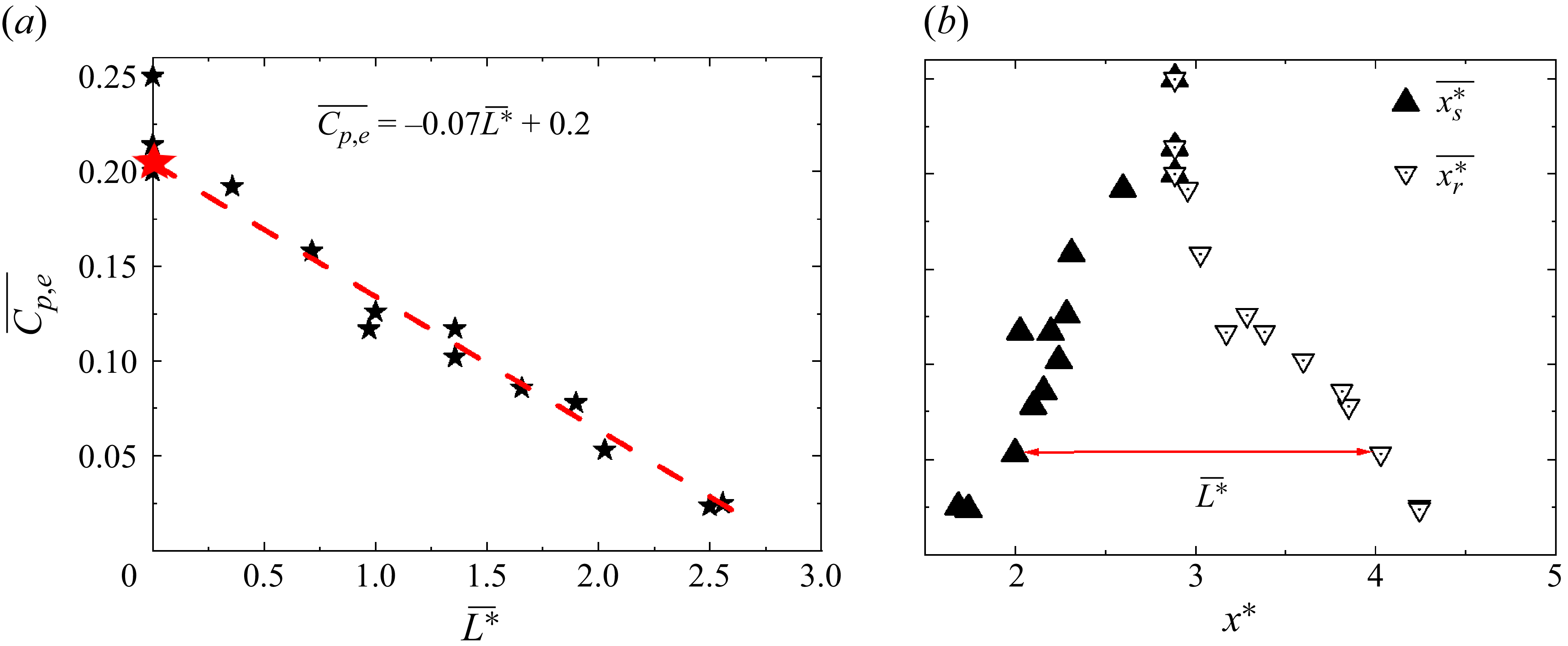In fact, the present data show that $\overline{L^{*}}$ and $\overline{C_{p,e}}$ are negatively correlated for $\alpha \leq 55^{\circ}$ (figure 4 a). As marked by the red star in figure 4(a), the recirculation region completely disappears at $\overline{C_{p,e}} \approx 0.2$ . As $\overline{C_{p,e}}$ increases, $\overline{x_{s}^{*}}$ shifts downstream and, meanwhile, the reattachment point $\overline{x_{r}^{*}}$ moves upstream (figure 4 b), resulting in a reduced $\overline{L^{*}}$ ( $\overline{L^{*}}=\overline{x_{r}^{*}}- \overline{x_{s}^{*}}$ ). Evidently, the variation in $\overline{C_{p,e}}$ , denoted by $\Delta \overline{C_{p,e}}$ , is an excellent indicator for the evaluation of control performance, viz.

(4.1) \begin{equation}\Delta \overline{C_{p,e}}=\overline{C_{p,e}}-\overline{C_{p,e}}_{0},\end{equation}

where $\overline{C_{p,e}}$ and $\overline{C_{p,e}}_{0}$ are the time-averaged pressure coefficient with and without control, respectively, at the end of ramp.

Figure 6.

Dependence of $(\Delta \overline{C_{p,e}})_{opt}$ on (a) $\overline{U_{J,c}^{*}}$ for various dc ( $\alpha$ = 0°, $f_{e}^{*}$ = 0.23), (b) dc for various $\overline{U_{J,c}^{*}}$ ( $\alpha$ = 0°, $f_{e}^{*}$ = 0.23) and (c) $\alpha$ for various dc ( $\overline{U_{J,c}^{*}}$ = 0.72, $f_{e}^{*}$ = 0.23).

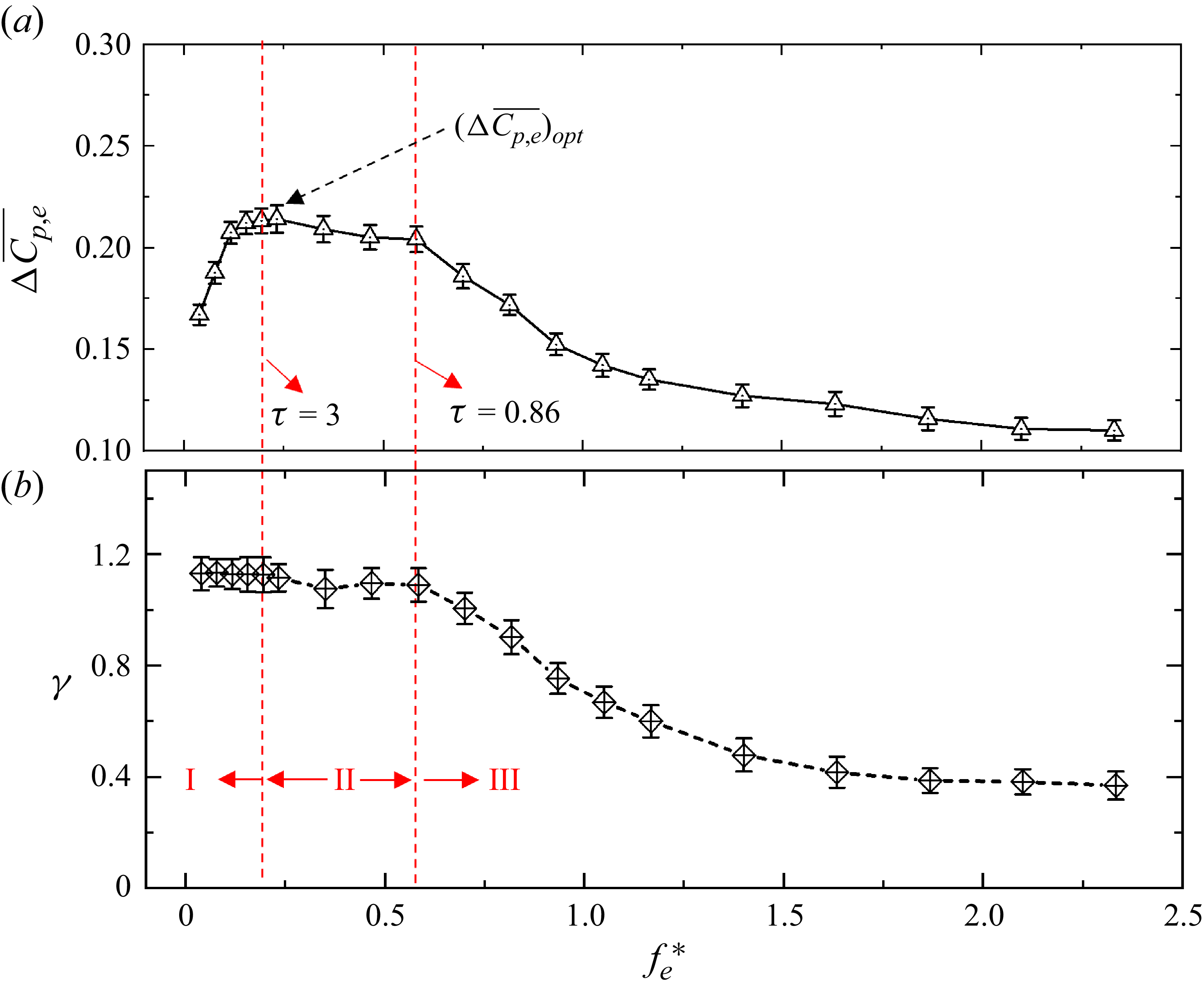
A parametric study is carried out to investigate the dependence of $\Delta \overline{C_{p,e}}$ on $\overline{U_{J,c}^{*}}$ , ${\rm d}c$ , $f_{e}^{*}$ and $\alpha$ . The relationship between $\Delta \overline{C_{p,e}}$ and $f_{e}^{{*}}$ is complicated (figure 5), and can be divided into three regions, i.e. I, II and III. In region I, $\Delta \overline{C_{p,e}}$ rises rapidly with increasing $f_{e}^{{*}}$ and the rising rate depends on dc. A smaller dc yields a more rapid rise. In region II, $\Delta \overline{C_{p,e}}$ changes little with increasing $f_{e}^{{*}}$ . In region III, $\Delta \overline{C_{p,e}}$ drops slowly with increasing $f_{e}^{{*}}$ and eventually levels off. It is worth noting that the critical $f_{e}^{{*}}$ at which region II changes to III varies with dc. For instance, as marked by the red dashed line, the critical $f_{e}^{{*}}$ is approximately 0.82 for dc = 0.3, but drops to 0.23 for dc = 0.8. However, $\tau$ remains constant, 0.86 at the point that separates regions II and III, and approximately 3 at the point that separates regions I and II, where

(4.2) \begin{equation}\tau =\frac{1-dc}{f_{e}^{*}}\end{equation}

represents the dimensionless duration during which the jet is closed in one period of the pulsed jet. Note that $(\Delta \overline{C_{p,e}})_{opt}$ in figure 5 is the $\Delta \overline{C_{p,e}}$ value at $f_{e}^{*}=0.23$ , at which the maximum $\Delta \overline{C_{p,e}}$ takes place for a given $\overline{U_{J,c}^{*}}$ and dc.

As shown in figure 6(a), $(\Delta \overline{{C}_{{p},{e}}})_{{opt}}$ rises monotonously with increasing $\overline{U_{J,c}^{*}}$ , regardless of dc, given $f_{e}^{*}$ and $\alpha$ since a large $\overline{U_{J,c}^{*}}$ enhances the Coanda effect, thus suppressing flow separation and promoting pressure recovery (He et al. Reference He, Zhang, Song and Zhou2023). Note that, limited by the solenoid valve used to produce the pulsed jet, there is a lack of data at very large $\overline{U_{J,c}^{*}}$ and small dc, e.g. at dc = 0.3 and 0.4 for $\overline{U_{J,c}^{*}}\geq 0.84$ . The relationship between $(\Delta \overline{{C}_{{p},{e}}})_{{opt}}$ and $\overline{U_{J,c}^{*}}$ is nonlinear, though qualitatively unchanged despite a variation in dc. However, given $f_{e}^{{*}}$ and $\alpha$ , $(\Delta \overline{{C}_{{p},{e}}})_{{opt}}$ drops monotonously and nonlinearly from dc = 0.3–0.9, irrespective of $\overline{U_{J,c}^{*}}$ (figure 6 b). For a fixed $\overline{U_{J,c}^{*}}$ or mass flow rate, a smaller dc will produce a larger maximum jet velocity (figure 2 c), thus enhancing the Coanda effect and causing a rise in $(\Delta \overline{{C}_{{p},{e}}})_{{opt}}$ . Additionally, $(\Delta \overline{{C}_{{p},{e}}})_{{opt}}$ exhibits a strong dependence on $\alpha$ (figure 6 c), dropping monotonously with increasing $\alpha$ for all dc. This is reasonable as a small $\alpha$ implies a larger tangential component of the jet and thus a stronger Coanda effect. The optimal control performance is achieved at $\alpha$ = 0°.

Figure 7.

PIV data with and without forcing: (a1) unforced instantaneous iso-contours of Q-Criterion superimposed with velocity vectors; (a2) unforced time-averaged streamlines superimposed with the velocity component $\overline{V^{*}}$ ; (b) time-averaged streamlines superimposed with $\overline{V^{*}}$ (forced at $\alpha$ = 0°, $\overline{U_{J,c}^{*}}$ = 0.59, dc = 0.3, $f_{e}^{*}$ = 0.25) when $\overline{C_{p,e}}(\approx 0.2)$ corresponds to the red star in figure 4(a); (c1–c5) phase-averaged streamlines superimposed with $\langle V^{*}\rangle$ . T is the period of the control jet, the red dashed curves represent the ramp and the red dot denotes the control jet position.

4.2. Control mechanism for $\alpha$ ≤ 55°

To gain an understanding of the flow physics and control mechanism, we analyse the PIV-measured velocity data in the x–y plane. In the baseline flow, a series of roller vortices originating from the Kelvin–Helmholtz instability are identified by Q-Criterion in figure 7(a1), and a recirculation region or separation bubble below these vortices is evident. The flapping of the vortices forms the high Reynold stresses and turbulent kinetic energy above the separation bubble. Inside the separation bubble, Reynold stresses and turbulent kinetic energy is relatively small (Song et al. Reference Song and Eaton2004; He et al. Reference He, Zhang, Song and Zhou2023). Under control ( $\alpha$ = 0°, $\overline{U_{J,c}^{*}}$ = 0.59, dc = 0.3 and $f_{e}^{*}$ = 0.25), the recirculation region, as shown in figure 7(a2) in the absence of control, vanishes completely, accompanied by a massive downward motion, as indicated by almost entirely negative $\overline{V^{*}}$ above the ramp (figure 7 b). The roller vortices also disappear due to the suppressed flow separation. The phase-averaged streamlines superimposed with $\langle$ V ^* $\rangle$ (figure 7 c1–c5) indicate that each jet injection generates one clockwise-rotating spanwise vortex downstream (figure 7 c1). This vortex grows when advected downstream (figure 7 c1–c2), though vanishing upon reaching the downstream plate surface (figure 7 c3–c5). A massive downward motion is generated upstream of this spanwise vortex, resulting in the flow attached to the wall.

Figure 8.

Schematic of the flow physics under control when the jet angle $\alpha$ = 0°–55°. Point O denotes the jet position. A small vortex A results from the interaction between the pulsed jet and the backflow. Blue arrows indicate the flow entrained from the mainstream into the jet.

A schematic is proposed in figure 8 on the physical mechanism of the suppressed flow separation from the ramp. The jet induces the Coanda effect, producing a low-pressure region between the jet and the wall with respect to the mainstream (Warsop et al. Reference Warsop and Crowther2018; Xu et al. Reference Xu, Su, Bensow and Krajnovic2022). The pressure difference between the mainstream and the near-wall region not only offsets the centrifugal force of the blowing jet (Englar Reference Englar2000), but also produces a massive downward fluid motion towards the curved ramp (figures 7 b and 7 c1–c5), forcing the separated flow attached to the wall. As a result, the recirculation region contracts and the pressure on the wall recovers. As the jet entrains fluid from only the upper side, i.e. the mainstream, unlike a free jet entraining fluid from both sides, the entrainment rate is higher than a free jet (Warsop et al. Reference Warsop and Crowther2018; Xu et al. Reference Xu, Qiao, Yang and Ye2018). Thus, the jet grows in width and its mean velocity decreases downstream at a higher rate than a free jet, which is associated with a pressure rise in the jet. When the pressure difference between the jet and the mainstream vanishes, the flow may separate again. Note that a small spanwise vortex A occurs downstream of the blowing jet, resulting from the interaction between the pulsed jet and the backflow near the wall due to flow recirculation. This vortex A is absent under steady jet control (He et al. Reference He, Zhang, Song and Zhou2023).

Figure 9.

(a) Schematic of the measurement positions; (b) dependence of $\overline{u^{2}}$ on the measurement position in the absence of control; (c) instantaneous iso-contours of Q-Criterion superimposed with velocity vectors under control; (d) pre-multiplied energy spectra of u measured at positions E and G in the baseline flow (d1–d2) and under control (d3–d4: $\alpha$ = 115°, $\overline{U_{J,c}^{*}}$ = 0.59, dc = 0.3, $f_{e}^{*}$ = 0.25).

4.3. Parametric study for $\alpha$ $\gt$ 55°

In this section, we examine closely the data of $\alpha \gt 55^{\circ}$ , where the $\overline{C_{p}}$ distributions display a difference in variation with $\overline{U_{J,c}^{*}}$ from those of $\alpha \leq 55^{\circ}$ (figure 3), suggesting different flow physics involved under control.

Let us first examine the pre-multiplied energy spectra of u measured in the absence of control. The measurement points A–K with 5 mm intervals along the y-direction are chosen at the end of the ramp (figure 9 a). Figure 9(b) is the dependence of $\overline{u^{2}}$ on y. As noted in the investigation on flow separation from a curved ramp by Song & Eaton (Reference Song and Eaton2004), the turbulence is inactive within the separation bubble, while the high turbulent kinetic energy region is caused by the flapping motion of roller vortices, resulting from the Kelvin–Helmholtz instability in the separated shear layer. The roller vortices are evident from the Q-Criterion (figure 7 a1). The pre-multiplied energy spectra (figure 9 d1–d2) of the baseline flow at positions E and G (figure 9 b), where $\overline{u^{2}}$ is large, display two appreciable peaks at f^* ≈ 0.04 and 0.25. The peak at f^* ≈ 0.04 is associated with the flapping motion or shear layer flapping, which is quite close to that observed by Chiatto, Luca & Grasso (Reference Chiatto, Luca de and Grasso2021) in a 3-D flow around a backward facing ramp, with a 25° slope angle. However, the peak at f^* ≈ 0.25 is due to the natural vortex shedding or roller vortices (figure 7 a1). Under control, the spectra (figure 9 d3–d4) display several differences. The spectral peak associated with flapping motion disappears completely. At $f_{e}^{*}=0.25$ , the spectrum shows a predominant and sharp peak at the excitation frequency, the other peak at higher frequency being its harmonic. This sharp peak is ascribed to the large-scale spanwise vortices generated by the control jet (figure 9 c). Apparently, the control suppresses the flapping motion on one hand and strengthens greatly vortex shedding on the other hand.

Figure 10.

(a) Dependence on $f_{e}^{*}$ and dc of space- and time-averaged pressure coefficient $\langle \overline{C_{p}}\rangle _{r}$ on the ramp ( $\alpha$ = 115°, $\overline{U_{J,c}^{*}}$ = 0.59); (b) longitudinal distributions of $\overline{C_{p}}$ for selected cases in (a) and baseline flow, where State 1 corresponds to the control under the optimal frequency and State 2 denotes the cases when control performance is independent of dc and $f_{e}^{*}$ .

Figure 11.

PIV time-averaged streamlines and iso-contours of $\overline{V^{*}}$ of (a) case P1 and (b) case P2; phase-averaged streamlines superimposed with $\langle V^{*}\rangle$ of (a1–a5) case P1 and (b1–b5) case P2. Red dashed curve represents the ramp and the red dot denotes the jet position.

Unlike the case of $\alpha \leq 55^{\circ}$ where a specific $\overline{C_{p,e}}$ or $\Delta \overline{C_{p,e}}$ corresponds to only one $\overline{C_{p}}$ distribution and hence one separation bubble size, one $\overline{C_{p,e}}$ may correspond to different $\overline{C_{p}}$ distributions for $\alpha \gt 55^{\circ}$ . One example is given in figure 10(b), where cases P1, P2 and P3 correspond to jet control at $f_{e}^{*}=0.25$ (synchronising with the natural vortex shedding frequency), 0.46 and 2.3, respectively (other control parameters are given in figure 10 a). Furthermore, the relationship between $\overline{C_{p,e}}$ and $\overline{L^{*}}$ in figure 4 does not hold anymore. As such, it would be inappropriate to use $\Delta \overline{C_{p,e}}$ as a valid indicator for control performance. Following Zhang et al. (Reference Zhang, Liu, Zhou, To and Tu2018) and Haffner et al. (Reference Haffner, Borée, Spohn and Castelain2020), we use the space- and time-averaged pressure coefficient $\langle \overline{C_{p}}\rangle _{r}$ as the indicator for control performance, which is defined by

(4.3) \begin{equation}\left\langle \overline{C_{p}}\right\rangle _{r}=\frac{1}{n}\sum _{k=1}^{n}\overline{C_{p,k}},\end{equation}

where n = 20 is the number of pressure taps on the ramp.

We examine $\langle \overline{C_{p}}\rangle _{r}$ only at $\alpha =115^{\circ}$ since the results are qualitatively similar for $\alpha =115^{\circ}$ , $85^{\circ}$ and 70°. The $\langle \overline{C_{p}}\rangle _{r}$ displays a dependence on $f_{e}^{*}$ and dc, especially about the optimal excitation frequency $f_{e}^{*}$ = 0.25. Away from 0.25, $\langle \overline{C_{p}}\rangle _{r}$ varies little with dc and $f_{e}^{*}$ , and depends on only $\overline{U_{J,c}^{*}}$ and $\alpha$ . Under control, $\overline{C_{p}}$ rises, compared with the uncontrolled case, and reaches its maximum at $x^{*}$ ≈ 1.65 where the control jet issues and then drops, especially at $f_{e}^{*}$ = 0.25 (case P1). The longitudinal $\overline{C_{p}}$ distribution at $f_{e}^{*}$   =  0.25 shows an appreciable difference from those, such as cases P2 and P3, away from 0.25. However, the $\overline{C_{p}}$ distributions corresponding to cases P2 and P3 collapse quite well. It is noteworthy that there is no similar optimal value of excitation frequency identified when $\alpha \leq 55^{\circ}$ .

4.4. Control mechanism for $\alpha$ $\gt$ 55°

To clear the flow physics for $\alpha \gt 55^{\circ}$ , the flow fields of cases P1 and P2 are presented in figure 11. Figures 11(a) and 11(b) show time-averaged streamlines superimposed with iso-contours of $\overline{V^{*}}$ for cases P1 and P2, respectively, and figures 11(a1–a5) and 11(b1–b5) present the corresponding phase-averaged streamlines superimposed with $\langle V^{*}\rangle$ . The two vortices in each plate of the phase-averaged data, such as vortices 1 and 6 in figure 11(a1), are generated by two consecutive jet pulses, because they have a time interval of 1.2T. In the adjacent plates, the corresponding two vortices, such as vortex 1 in figure 11(a1) and vortex 2 in figure 11(a2), have a time interval of 0.2T. This suggests that they are from the same jet pulse, occurring at different moments. After the spanwise vortex is generated at the jet exit, its lifecycle or motion follows the sequence of 1 → 2 → 3 → 4 → 5 → 6 → 7 → 8 → 9 → 10 (figure 11 a1–a5). As the vortex moves downstream, its core intensity keeps impairing; its size grows from 1 to 6 and then contracts from 7 to 10 before eventual vanishment downstream. Each pulse of the slit jet generates a large spanwise vortex (figure 11), as produced by the synthetic jet issued from a slit (Dandois et al. Reference Dandois, Garnier and Sagaut2007), which is different from a hairpin vortex or distorted vortex-ring produced by circular synthetic jets (Palumbo et al. Reference Palumbo, Semeraro, Robinet and Luca de2022). When the pulsed-jet frequency is close to the natural vortex shedding frequency (case P1), the spanwise vortex is significantly intensified, as shown in figure 11(a1–a5) (cf. figure 11 b1–b5). Upwash flow is formed on the left side of the vortex core, while downwash flow is generated on the right side (figure 11 a1–a5). This leads to strong momentum transfer, hence resulting in a slight reduction in the recirculation region (figure 11 a). Zhang & Zhong (Reference Zhang and Zhong2011) also observed in the control of flow separation from a curved ramp that the jet-generated hairpin vortices are significantly intensified when the actuation frequency of the round-hole synthetic jet is close to the natural shedding frequency. In the study on flow separation control over a wall-mounted hump, Greenblatt et al. (Reference Greenblatt, Paschal, Yao and Harris2006) found that when the spanwise slot synthetic jets are operated near the shear layer frequency, the spanwise vortices produced by the jets may merge with the shedding vortices to form larger-scale spanwise vortical structures, which postpones flow separation. For actuation frequency away from the natural shedding frequency, such as case P2, the jet also generates spanwise vortices. Unlike those in case P1, the vortices in case P2 are significantly weaker and dissipate rapidly when moving downstream (figure 11 b1–b5), failing to create as strong a momentum exchange as in case P1 (figure 11 a1–a5). However, as shown by He et al. (Reference He, Zhang, Song and Zhou2023), the upward jet injects momentum into the incoming shear layer and behaves as a tiny spoiler. Please refer to the zoom-in part of figure 11(a–b). This effect results in the separating shear layer deviating away from the wall. Consequently, the corresponding reattachment points shift substantially downstream and the separation bubble enlarges in case P2.

Figure 12.

Schematic of flow physics under control when the jet angle $\alpha \gt 55^{\circ}$ : (a–b) pulsed jet; (c) steady jet. The green arrows denote the upwash and downwash flows generated by spanwise vortices. The red solid curves with an arrow indicate the recirculation region under control. The red and blue dashed lines represent the shear layers with and without control, respectively. The black solid arrows represent the jet directions.

Combining cases P1 and P2 of pulsed jet control as well as steady jet control (He et al. Reference He, Zhang, Song and Zhou2023) for $\alpha \gt 55^{\circ}$ , a conceptual schematic is summarised in figure 12. The pulsed control jet produces two effects. First, the upward jet injects momentum into the incident shear layer and acts to enlarge the separation bubble (control effect 1). Second, the jet generates a clockwise spanwise vortex, acting to enhance momentum transfer and to reduce the separation bubble size (control effect 2). For steady jet control, there is only the former effect and thus the separation bubble grows (figure 12 c). In case P1 of the pulsed jet control, the spanwise vortices are markedly strengthened when the excitation frequency is close to the natural vortex shedding frequency. As such, the latter effect dominates and the separation bubble contracts slightly (figure 12 a). In case P2, the former effect dominates since the spanwise vortices are relatively weak, thus causing the separation bubble to grow (figure 12 b).

5.1. Analysis of $\overline{U_{J,c}^{*}}$ and dc

An empirical scaling analysis is performed for $\alpha \leq 55^{\circ}$ in this section. Valuable insight into the flow physics and control mechanisms behind the influence of control parameters on flow separation may be gained from this analysis.

The energy ratio $\gamma $ of the control jet to the mainstream per unit area may be given by

(5.1) \begin{equation}\gamma =\frac{\big(\int _{0}^{nT}0.5 \dot{m}_{\infty } U_{J,c}^{2}{\rm d}t\big)/nT}{\big(\int _{0}^{nT}0.5\dot{m}_{J,c} U_{\infty }^{2} {\rm d}t\big)/nT}=\frac{\overline{U_{J,c}^{3}}}{U_{\infty }^{3}}=\overline{U_{J,c}^{*3}},\end{equation}

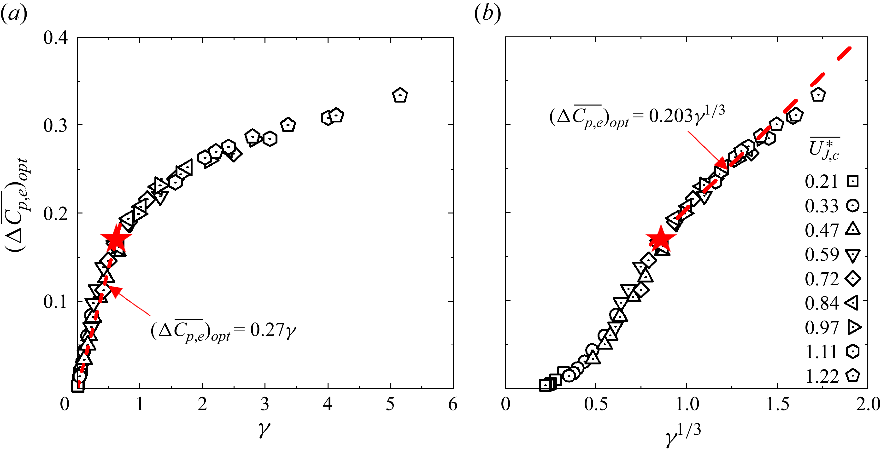
where n represents the cycle number of the pulsed jet ( $n\geq 100$ ), T is the period of the control jet, $\dot{m}_{\infty }=\rho U_{\infty }$ and $\dot{m}_{J,c}=\rho U_{J,c}$ are the mass flow rates per unit area of main flow and jet, respectively, and $0.5\dot{m}_{J,c}U_{J,c}^{2}$ and $0.5\dot{m}_{\infty }U_{\infty }^{2}$ are the instantaneous power per unit area of the jet and main flow, respectively. After careful theoretical and experimental data analyses, it has been found that all the data points of $(\Delta \overline{{C}_{{p},{e}}})_{{opt}}$ in figure 6(a–b) collapse about a curve, regardless of $\overline{U_{J,c}^{*}}$ and dc, once being presented as the function of  $\gamma $ (figure 13 a) or $\gamma ^{1/3}$ (figure 13 b). The observation suggests that $\gamma $ is the controlling scaling factor; that is, $(\Delta \overline{{C}_{{p},{e}}})_{{opt}}$ or the separation bubble size is the same for a fixed  $\gamma $ , irrespective of different mean velocity ratio and duty cycle. Note that a larger mean velocity ratio or smaller duty cycle leads to a larger $\gamma $ and hence a larger $(\Delta \overline{{C}_{{p},{e}}})_{{opt}}$ . This explains why $(\Delta \overline{{C}_{{p},{e}}})_{{opt}}$ rises monotonically with increasing mean velocity ratio and decreasing duty cycle (figure 6 a–b).

Figure 13.

Dependence of $(\Delta \overline{C_{p,e}})_{opt}$ on (a) the jet energy ratio $\gamma$ and (b) $\gamma ^{1/3}$ , including all data points in figure 6(a–b) ( $\alpha$ = 0°, $f_{e}^{*}$ = 0.23, dc = 0.3, 0.4, …, 0.9). The red dashed curves in panels (a) and (b) are least-squares fitting to data points at $\gamma$ $\lt$ 0.7 and $\gamma$ ≥ 0.7, respectively. The red star, corresponding to the red star in figure 4, represents the critical point where the separation bubble disappears.

Figure 14.

(a) Hotwire-measured time history of $U_{J,c}$ ( $\overline{U_{J,c}^{*}}$ = 0.72, dc = 0.3, $f_{e}^{*}$ = 0.23), where the red-colored curve is the theoretical time history calculated from dc and $\overline{U_{J,c}}$ , as indicated by the horizontal blue line; (b) correlation between the effective duty cycle $dc_{e}$ and dc.

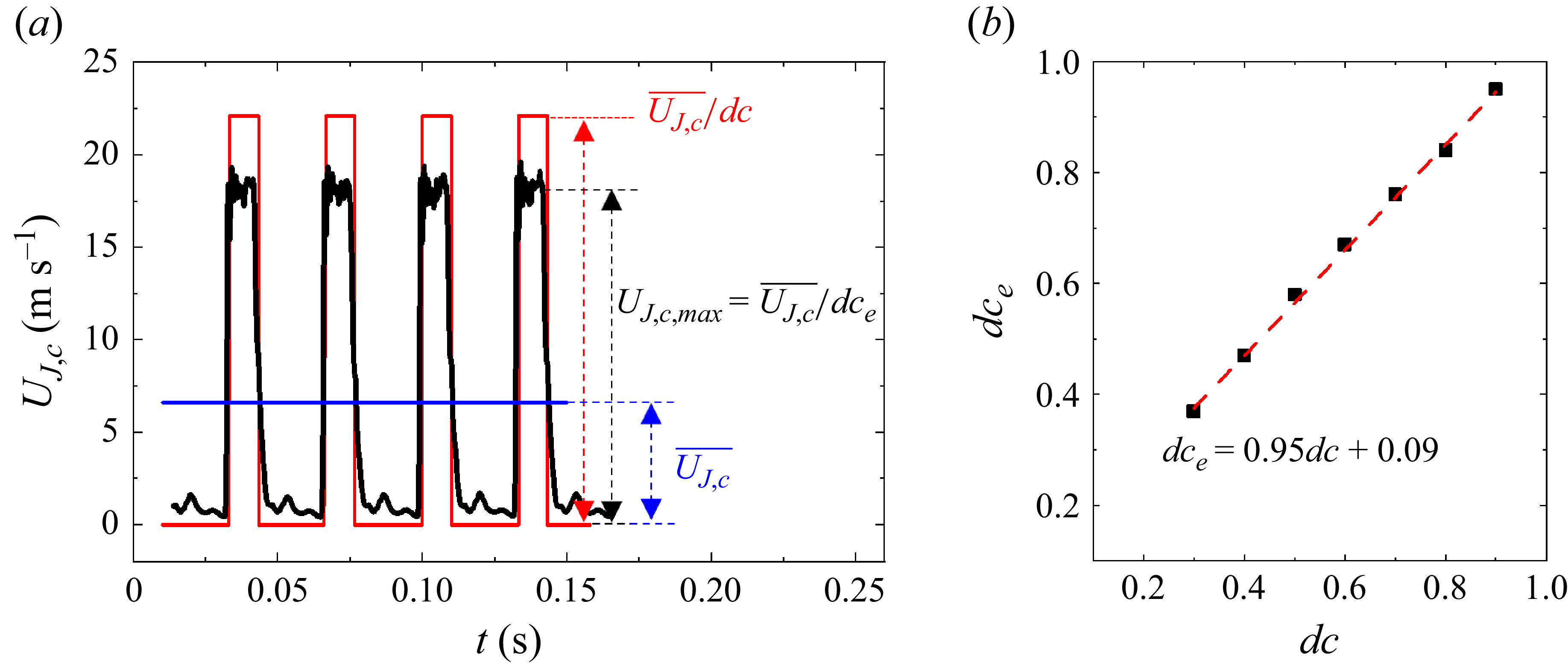
Since energy ratio $\gamma $ is obtained from hot-wire measurement and depends on mean velocity ratio and duty cycle, one question arises. Can $\gamma $ be expressed as a combination of mean velocity ratio and duty cycle? As indicated by the red solid curve in figure 14(a), if the time history of the jet velocity is an ideal square wave, (5.1) can be theoretically rewritten as

(5.2) \begin{equation}\text{Energy ratio}=\frac{\big(\int _{0}^{nT}0.5 m_{J,c} U_{J,c}^{2} {\rm d}t\big)/nT}{\big(\int _{0}^{nT}0.5 m_{\infty } U_{\infty }^{2} {\rm d}t\big)/nT}=\frac{\left(\frac{\overline{U_{J,c}}}{{\rm d}c}\right)^{3} {\rm d}c n T}{U_{\infty }^{3} n T}=\frac{\overline{U_{J,c}^{*}}^{3}}{{\rm d}c^{2}},\end{equation}

where $\overline{U_{J,c}}/{ d}c$ is the nominal maximum value of the jet velocity. However, the actually measured instantaneous maximum value $U_{J,c,max}$ , as shown by the black solid curve in figure 14(a), is smaller than the nominal maximum value because of the limitation of the present state-of-the-art technology of solenoid valves and the inertia of the air in the tube. As such, dc in (5.2) should be replaced by an effective duty cycle $dc_{e}$ , which is defined by

(5.3) \begin{equation}U_{J,c,\textit{max}}=\frac{\overline{U_{{J,c}}}}{{ d}c_{e}}. \end{equation}

As shown in figure 14(b), with $\overline{U_{J,c}^{*}}^{3}/{ d}c^{2}$ replaced by $\overline{U_{J,c}^{*}}^{3}/{ d}c_{e}^{2}$ , dc and $dc_{e}$ are linearly correlated, viz.

(5.4) \begin{equation}{ d}c_{e}=0.95{ d}c+0.09.\end{equation}

Equation (5.4) differs from the correlation between dc and $dc_{e}$ reported by Fan et al. (2023). This deviation may result from the different systems producing the pulsed jet. In their study, the minijet from the solenoid valve is directly injected into the main jet, while the present pulsed jet first flows into an actuator chamber after the solenoid valve (figure 1 b) and then is injected into the mainstream.

Figure 15.

Comparison between the dependences of $(\Delta \overline{C_{p,e}})_{opt}$ on $\gamma$ and $\overline{U_{J,c}^{*}}^{3}/{ d}c_{e}^{2}$ ( $\alpha$ = 0°, $f_{e}^{*}$ = 0.23, dc  = 0.3, 0.4, …, 0.9).

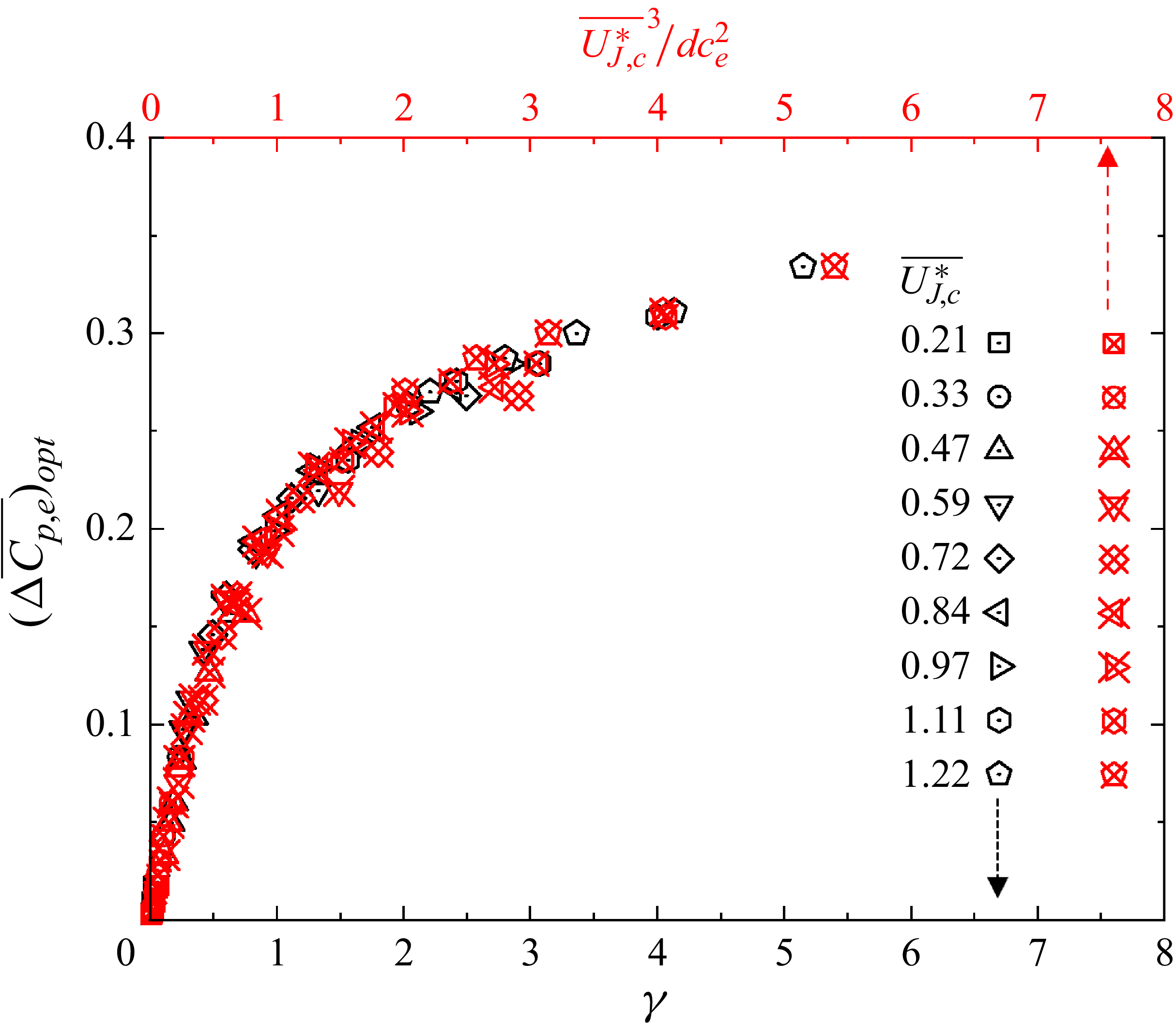
We now use $\overline{U_{J,c}^{*}}^{3}/{ d}c_{e}^{2}$ as the abscissa and then observe that the correlation between $(\Delta \overline{{C}_{{p},{e}}})_{{opt}}$ and $\overline{U_{J,c}^{*}}^{3}/{ d}c_{e}^{2}$ overlaps reasonably well with that between $(\Delta \overline{{C}_{{p},{e}}})_{{opt}}$ and $\gamma$ (figure 15). Note that the premise of (5.2) is that the time history of the jet velocity follows the square wave, which is achievable only at a low excitation frequency. At a high frequency, the time history of the jet velocity cannot be approximated as a square wave and  $\gamma$ cannot be written as $\overline{U_{J,c}^{*}}^{3}/{ d}c_{e}^{2}$ . Two important inferences can be made from figure 15. First, the scaling factor $\gamma$ is equivalent to $\overline{U_{J,c}^{*}}^{3}/{ d}c_{e}^{2}$ at a low excitation frequency. This is because the time history of the jet velocity at a low frequency can be approximated as a square wave and $dc_{e}$ and dc are linearly correlated (figure 14). Second, while a great amount of hotwire data is required to determine $\gamma$ , $\overline{U_{J,c}^{*}}^{3}/{ d}c_{e}^{2}$ can be directly calculated from the control parameters and (5.4). As found by Perumal & Zhou (Reference Perumal and Zhou2018), scaling factor $\overline{U_{J,c}^{*}}^{3}/{ d}c_{e}^{2}$ is important in engineering applications, which can be used to predict $(\Delta \overline{{C}_{{p},{e}}})_{{opt}}$ or to determine the control parameters.

5.2. Analysis of $f_{e}^{*}$ and $\alpha$

The scaling shown in figures 13 or 15 is obtained at $f_{e}^{*}$ = 0.23. One may wonder whether $\Delta \overline{C_{p,e}}$ would also collapse when excitation frequency varies, with $\gamma$ remaining as the scaling factor. Figure 16 presents the variation in $\gamma$ and $\Delta \overline{C_{p,e}}$ with excitation frequency at dc = 0.5 and $\overline{U_{J,c}^{*}}=0.72$ . In regions II and III, the dependence of $\gamma$ on excitation frequency exhibits excellent similarity to that of $\Delta \overline{C_{p,e}}$ . Furthermore, the critical $\tau$ where region II changes to region III is 0.86, the same as in figure 5. However, the variations in  $\gamma$ and $\Delta \overline{C_{p,e}}$ with excitation frequency display a marked difference in region I; $\Delta \overline{C_{p,e}}$ rises rapidly with excitation frequency, whilst $\gamma$ varies little. The result suggests that the way excitation frequency influences $\Delta \overline{C_{p,e}}$ in regions II and III may result, via the relation between $\Delta \overline{C_{p,e}}$ and $\gamma$ (figures 13 or 15), from the variation in $\gamma$ with excitation frequency, whereas in region I, there may be other controlling factors at play besides $\gamma$ .

Figure 16.

Dependence on $f_{e}^{{*}}$ of (a) $\Delta \overline{C_{p,e}}$ and (b) $\gamma$ ( $\overline{U_{J,c}^{{*}}}=0.72$ , dc = 0.5, $\alpha$ = 0°). The error bars denote the standard deviation out of 10 repeated measurements. The vertical red broken lines indicate a division that separates regions I and II or II and III.

The above-mentioned speculation is indeed confirmed. Figure 17 presents the dependence of $\Delta \overline{C_{p,e}}$ on $\gamma$ , including all the data at $\alpha =0^{\circ}$ in figure 5(a,b) and 6. All of the data points in regions II and III collapse well about the red broken curve, but not those in region I, as shown by the blue symbol, which shows a large departure from the curve. This result points unequivocally to the fact that in contrast to regions II and III, $\Delta \overline{C_{p,e}}$ depends not only on $\gamma$ , but also on other factors. This observation raises two issues. One is why $\gamma$ exhibits little dependence on excitation frequency in the low frequency range, or regions I and II (figure 16), but drops with rising excitation frequency in the high frequency range, or region III. The other is what factors, apart from $\gamma$ , play a non-negligible role in region I.

Figure 17.

Dependence of $\Delta \overline{C_{p,e}}$ on $\gamma$ ( $\alpha$ = 0°), including all data points in figures 5 and 6(a,b). The blue and black symbols denote data points in region I ( $\tau \gt 3$ ) and regions II, III ( $\tau \leq 3$ ), respectively. The latter fall around a red broken curve, which is the least-squares-fitting curve to the data.

To address the first issue, let us take a close look at the data of jet velocity at dc = 0.5 and $\overline{U_{J,c}^{{*}}}=0.72$ . Figure 18(a) presents the variations with excitation frequency in the root mean square (r.m.s.) value $U_{J,c}^{\prime*}$ of the jet velocity (left ordinate) and the corresponding  $\gamma$ (right ordinate). The two curves are almost parallel to each other; $U_{J,c}^{\prime*}$ and $\gamma$ display a small variation with excitation frequency at $f_{e}^{*}\leq 0.58$ or $\tau$ ≥ 0.86 (regions I and II) but both drop and then eventually level off at $f_{e}^{*}\gt 0.58$ (region III). Figure 18(b) shows the phase-averaged time histories of the jet velocity at five representative frequencies, i.e. $f_{e}^{*}=0.04, 0.23, 0.58, 1.17, 2.33$ . The time t is normalised by the period T of the pulsed jet. The time histories are approximately square waves at $f_{e}^{*}=0.04$ , 0.23 and 0.58, and their maximum and minimum values are almost the same. As excitation frequency increases beyond $f_{e}^{*}=0.58$ , the time history changes from a square-wave-like to a sinusoidal-wave-like signal at $f_{e}^{*}=1.17$ or 2.33. The corresponding maximum value drops, while the minimum value rises markedly, thus leading to a reduced magnitude in the jet velocity or $\gamma$ . In summary, the time history of the jet velocity is approximately a square wave in regions I and II ( $\tau \geq 0.86$ ), and the corresponding maximum, minimum and r.m.s. values vary little for different excitation frequencies. Consequently, $\gamma$ is independent of excitation frequency and can be rewritten as $\overline{U_{J,c}^{*}}^{3}/{ d}c_{e}^{2}$ , as shown in figure 14. In region III ( $\tau \lt 0.86$ ), the variation in r.m.s. value or time history of the jet velocity with excitation frequency results in a change in $\gamma$ , which is responsible for the decrease in $\Delta \overline{C_{p,e}}$ with excitation frequency (figure 5).

Figure 18.

(a) Dependence on $f_{e}^{*}$ of $U_{J,c}^{\prime*}$ and $\gamma$ ; (b) time histories of $\langle U_{J,c}^{*}\rangle$ at different $f_{e}^{*}$ (dc = 0.5, $\overline{U_{J,c}^{*}}$   = 0.72).

The jet exit velocity generated in experiments may change from the characteristics of a square wave to those of a sinusoidal wave with increasing excitation frequency due to viscous losses and jet inertia (Barros et al. Reference Barros, Ruiz, Borée and Noack2014, Reference Barros, Borée, Noack, Spohn and Ruiz2016), and accordingly, its magnitude diminishes as well. It is further found that the frequency, where the wave shape starts to show appreciable change, varies with the duty cycle, but $\tau$ would not. The present critical  $\tau$ of 0.86 may depend on the system that generates the pulsed jet, including the position and response time of the solenoid valve in the supply line, the design of plenum and so on. In their numerical investigation on wing circulation control, Liu et al. (Reference Liu, Sankar, Englar, Ahuja and Gaeta2004) found that the square wave was more effective than the sinusoidal wave. Given a lift coefficient, the required mass flow rate for the sinusoidal pulsed jet was much higher than that for the square-wave jet. This is, as shown in figure 18, because a square-wave jet is associated with a higher $\gamma$ than a sinusoidal wave jet, even under the same mass flow rate.

Figure 19.

Dependence of $\Delta \overline{C_{p,e}}/\varPi (\tau )$ on (a) $\gamma$ ( $\alpha$ = 0°, $\gamma$ $\lt$ 0.7) and (b) $\gamma ^{1/3}$ ( $\gamma$ ≥ 0.7), where the red dashed curve is the least-squares fitting to data points. The blue and black symbols denote data points in region I ( $\tau \gt 3$ ) and regions II, III ( $\tau \leq 3$ ), respectively. The red star, corresponding to the red star in figure 4, represents the critical point where the separation bubble disappears.

To address the second issue, we carefully analyse the data points in region I (blue symbols in figure 17), which exhibit a significant departure from those in regions II and III. It is found that once $\Delta \overline{C_{p,e}}$ is rescaled by $\varPi (\tau )$ , as shown in figure 19, all data points at various $\overline{U_{J,c}^{{*}}}$ , dc and $f_{e}^{{*}}$ collapse well about a piecewise least-square fitting curve, viz.

(5.5) \begin{equation}\Delta \overline{C_{p,e}}/\varPi \left(\tau \right)=\begin{cases} 0.27 \gamma ,& \gamma \lt 0.7,\\ 0.203 \gamma ^{1/3}, & \gamma \geq 0.7, \end{cases}\end{equation}

where $\varPi (\tau )$ is a function of $\tau$ , given by

(5.6) \begin{equation}\varPi \left(\tau \right)=\begin{cases} 1 ,& \tau \leq 3,\\ -0.021\tau +1.06, & \tau \gt 3. \end{cases}\\[-6pt]\nonumber \end{equation}

When $\tau \gt 3$ (region I), $\varPi (\tau )\neq 1$ and $\Delta \overline{C_{p,e}}$ (blue symbols) depend on not only $\gamma$ but also $\tau$ or $\varPi (\tau )$ ; when $\tau \leq 3$ (regions II and III), $\varPi (\tau )\equiv 1$ and $\Delta \overline{C_{p,e}}$ (black symbols) depend only on $\gamma$ since $\tau$ is so small that its effect may be neglected. It is noteworthy that the data points in region I of figure 17 scatter rather wildly because the presented $\Delta \overline{C_{p,e}}$ = f ( $\gamma$ ) does not include the possible effect of $\tau$ .

The relation ‘ $\Delta \overline{C_{p,e}}/\varPi (\tau )=f_{2}(\gamma )$ ’ in figure 19 may be rewritten as $\Delta \overline{C_{p,e}}=\varPi (\tau )f_{2}(\gamma )$ . As shown in figure 20, $\Delta \overline{C_{p,e}}$ can be then divided into two regimes, i.e. $\Delta \overline{C_{p,e}}=0.27\varPi (\tau )\gamma$ for $\varPi (\tau )\gamma \lt 0.7$ and $\Delta \overline{C_{p,e}}=0.203\varPi (\tau )\gamma ^{1/3}$ for $\varPi (\tau )\gamma \geq 0.7$ , corresponding to before and after the disappearance of the separation bubble. Apparently, $\varPi (\tau )$ is physically an indicator for the control efficiency which depends on only $\tau$ .

Figure 20.

Dependence of $\Delta \overline{C_{p,e}}$ on $\varPi (\tau )\gamma$ and $\varPi (\tau )\gamma ^{1/3}$ ( $\alpha$ = 0°). The red dashed lines are the least-squares fitting to data points. The red star is the same as in figure 19.

Insight may be gained into how $\tau$ may affect $\Delta \overline{C_{p,e}}$ in region I by the analysis of the time histories of $\langle C_{p,e}\rangle$ along with $\langle U_{J,c}^{*}\rangle$ . Consider two different combinations of $\tau$ and $\varPi (\tau )$ in figure 21, i.e. case 1 ( $\tau$ = 12.8, $\varPi (\tau )=0.79$ ) from region I and case 2 ( $\tau$ = 2.2, $\varPi (\tau )=1$ ) from region II. The time histories of $\langle U_{J,c}^{*}\rangle$ are square-wave-like, and display a reasonably good overlap in terms of the jet-on and -off durations for the two cases when normalised by the period T of the pulsed jet (figure 21 a). Their peaks and valleys are comparable, thus producing the same $\gamma$ ( =  1.13), which facilitates the study of the effect of $\tau$ on $\Delta \overline{C_{p,e}}$ . The time histories of $\langle C_{p,e}\rangle$ for the two cases are characterised by approximately the same peak value but very different troughs (figure 21 b). With a small  $\tau$ , case 2 features a higher trough value than case 1, thus a larger $\Delta \overline{C_{p,e}}$ . When the jet is turned off and $\langle U_{J,c}^{*}\rangle$ falls, $\langle C_{p,e}\rangle$ starts to drop and finally reaches its trough. When the jet is turned on again, with $\langle U_{J,c}^{*}\rangle$ rising, in the next cycle of the jet, $\langle C_{p,e}\rangle$ rises and reaches the peak at the end of a duration ${d}c/f_{e}^{*}$ . In case 1, $\langle C_{p,e}\rangle$ descends to a value comparable to the baseline flow due to a larger $\tau$ ( =  12.8), suggesting flow separation again and the Coanda effect disappears almost completely before the next cycle. In case 2, once the jet is off, $\langle C_{p,e}\rangle$ also drops but could not reach the same trough as the baseline flow because of a small $\tau$ ( =  2.2). Consequently, flow separation is always suppressed, at least partially, during the entire excitation period. Then, it seems plausible that a sufficiently small $\tau$ , i.e. in regions II and III where $\tau$ ≤ 3, may take advantage of jet inertia to sustain continuously the Coanda effect, thus maintaining $C_{p,e}$ at a higher level even when the jet is turned off. If a new blowing cycle starts under such circumstances, the Coanda effect may immediately recover itself towards the optimal state achievable for a given jet energy. This physical process underpins the rapid rise in $\Delta \overline{C_{p,e}}$ with increasing excitation frequency in region I (figure 5).

Figure 21.

Time histories of (a) $\langle U_{J,c}^{*}\rangle$ and (b) corresponding $\langle C_{p,e}\rangle$ for $\tau$ = 12.8 and 2.2 ( $\alpha$ = 0°, $\overline{U_{J,c}^{*}}$ = 0.72, dc = 0.5), along with the uncontrolled case.

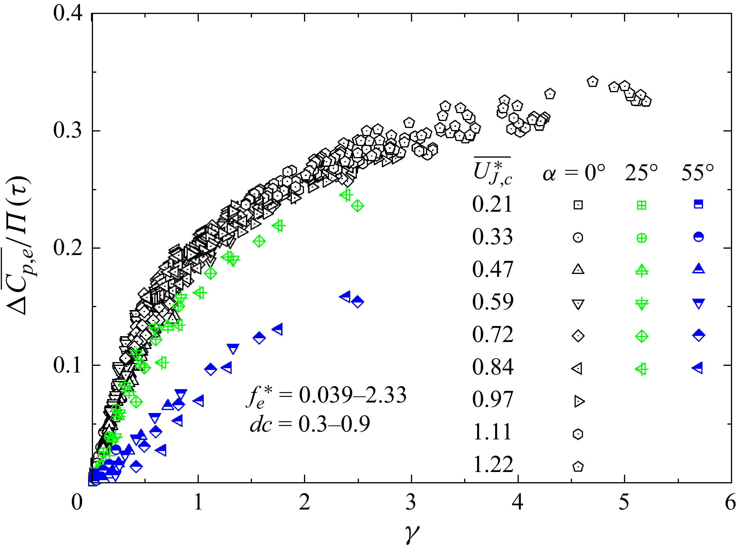
The scaling analysis shown in figure 19 is obtained at $\alpha$ = 0°. As shown in figure 22, a similar collapse is observed at $\alpha$ = 25° and 55° when the data are plotted against $\gamma$ . Given $\gamma$ , the smaller the $\alpha$ , the larger the $\Delta \overline{C_{p,e}}$ , which reaches the maximum at $\alpha$ = 0°. One may wonder whether a scaling law is present even when $\alpha$ varies. After careful analysis along with numerous trial-and-error attempts, it is found that $\Delta \overline{C_{p,e} }/\varPi(\tau )$ of all  $\alpha$ collapse around a curve provided that $\gamma$ in figure 22 is replaced by $\xi$ (figure 23), viz.

Figure 22.

Dependence of $\Delta \overline{C_{p,e}}/\varPi (\tau )$ on $\gamma$ for various α.

Figure 23.

Dependence of $\Delta \overline{C_{p,e}}/\varPi (\tau )$ on $\xi$ , where the red broken curve is the least-squares fitting to the measured data. The red star is as in figure 20.

(5.7) \begin{equation}\Delta \overline{C_{p,e}}/\varPi (\tau )=\begin{cases} 0.27 \xi , & \xi \lt 0.7,\\ 0.203 \xi , & \xi \geq 0.7, \end{cases}\end{equation}

where the scaling factor $\xi$ is defined by

(5.8) \begin{equation}\xi =\overline{U_{J,c,t}^{*3}}\end{equation}

and

(5.9) \begin{equation}U_{J,c,t}^{*}=U_{J,c}^{*}\cos\alpha =\frac{U_{J,c}\cos \alpha }{U_{\infty }}.\end{equation}

Equation (5.7) is the same in form as (5.5), including the turning point position.

5.3. Relationship between steady and pulsed jet controls and $ \textit{Re}_{\theta }$ effect

He et al. (Reference He, Zhang, Song and Zhou2023) manipulated the same flow using a steady blowing jet. One may naturally wonder whether the scaling law (5.7) could be applied to the case of steady control since the unsteady control approaches steady when excitation frequency becomes very large, as suggested by figure 18(b). Figure 24(a) presents the dependence of $\Delta \overline{C_{p,e}}$ on $\overline{U_{J,c}^{*}}$ and $ \textit{Re}_{\theta }$ ( ${=}5700{-}12\,200)$ using a steady control jet at $\alpha$ = 0° and 25°. As found by He et al. (Reference He, Zhang, Song and Zhou2023), the data points at different $ \textit{Re}_{\theta }$ collapse reasonably well about a curve for a given jet angle if plotted against $\overline{U_{J,c}^{*}}$ . Interestingly, the data points from steady jet control collapse well with the present data under the pulsed jet control, irrespective of $\alpha$ and $ \textit{Re}_{\theta }$ , when $\xi$ is used as the scaling factor (figure 24 b). The observation suggests that the scaling law is applicable for not only pulsed jet control but also steady jet control. The latter is a special case of the former, where $\tau$ = 0, $\varPi(\tau )=1$ in (5.6) and $\xi =\overline{U_{J,c,t}^{*3}}=\overline{U_{J,c,t}^{*}}^{3}$ ( $\xi =\overline{U_{J,c,t}^{*3}}\neq \overline{U_{J,c,t}^{*}}^{3}$ for a pulsed control jet). As a result, this scaling law can be simplified to $\Delta \overline{C_{p,e}}=f_{3}(\overline{U_{J,c}^{*}})$ for a steady control jet at a given jet angle, as found by He et al. (Reference He, Zhang, Song and Zhou2023). As another note, although the data of $\Delta \overline{C_{p,e}}$ against $\overline{U_{J,c}^{*}}$ display a quite good collapse about a curve in figure 24(a), the scaling law shown in figure 24(b) contains richer information on top of its broader applicability. Take the turning point marked by a star in figure 24(b) for example. This point corresponds to the control state where the separation bubble just disappears. The pressure recovers rapidly and linearly with $\xi$ before reaching this point due to a contraction in the separation bubble size, but slowly beyond this point.

Figure 24.

(a) Dependence of $\Delta \overline{C_{p,e}}$ on the velocity ratio $\overline{U_{J,c}^{*}}$ of steady jet control at various $ \textit{Re}_{\theta }$ . The data of steady control at $\alpha =25^{\circ}$ are from He et al. (Reference He, Zhang, Song and Zhou2023) and those of $\alpha =0^{\circ}$ are the present data; (b) dependence of $\Delta \overline{C_{p,e}}/\varPi (\tau )$ on $\xi$ , including the data of both steady and pulsed jet controls, where the red dashed curve is the least-squares fitting to the measured data. The red star is the same as in figures 19 and 23.

It is well known that $\Delta \overline{C_{p,e}}$ depends on $\overline{U_{J,c}^{*}}$ , ${\rm d}c$ , $f_{e}^{*}$ , $\alpha$ and $ \textit{Re}_{\theta }$ i.e.

(5.10) \begin{equation}\Delta \overline{C_{p,e}}=f_{1}\big(\overline{U_{J,c}^{*}}, { d}c, f_{e}^{*}, \alpha , Re_{\theta }\big).\end{equation}

As shown in figure 24(b), this highly complex relationship is now reduced to

(5.11) \begin{equation}\Delta \overline{C_{p,e}}/\varPi (\tau )=f_{2}\left(\xi \right).\end{equation}

This scaling law provides not only valuable insight into the flow physics behind control, but also important guidance for the choice of control parameters and the prediction of control performance. First, this scaling law may be written as $\Delta \overline{C_{p,e}}=0.27 \varPi(\tau ) \xi$ and $0.203 \varPi(\tau ) \xi ^{1/3}$ , corresponding to before and after the disappearance of the separation bubble, respectively. We see immediately that the factor $0.27 \varPi (\tau )$ can be understood to be the end pressure coefficient rise for each unit energy input associated with the tangential jet velocity $U_{J,c,t}^{*}$ , that is, $\varPi (\tau )$ is an indicator of the control efficiency. Second, the duration  $\tau$ plays an important role in determining the control performance. Here, $\varPi (\tau )$ is a function of $\tau$ . In regions II and III, $\tau$ (≤ 3) is so small that its effect on $\Delta \overline{C_{p,e} }$ can be neglected. Thus, $\varPi (\tau )\equiv 1$ and $\Delta \overline{C_{p,e} }$ depends only on $\xi$ (figures 19 and 20). In region I, $\tau$ $\gt$ 3 and $\varPi (\tau )$ drops linearly with increasing $\tau$ ( 5.6) and $\Delta \overline{C_{p,e}}$ depends not only on $\xi$ but also on $\tau$ (figures 19 and 20), and a larger $\tau$ will result in a smaller $\Delta \overline{C_{p,e}}$ for a fixed  $\xi$ (figure 21). Third, the optimal control strategy is that the jet is injected tangentially, i.e. at $\alpha$ = 0° (figure 22), and at $\tau$ = 0.86–3, i.e. in region II (figure 5). For tangential jet control in region II where $\xi =\gamma =\overline{U_{J,c}^{*}}^{3}/{ d}c_{e}^{2}$ holds, given $\overline{U_{J,c}^{*}}$ and ${ d}c$ , $\overline{U_{J,c}^{*}}^{3}/{ d}c_{e}^{2}$ may be directly calculated and hence $\Delta \overline{C_{p,e}}$ can be predicted from (5.7). This may have important applications in engineering. Conversely, the required $\overline{U_{J,c}^{*}}$ to achieve a pre-specified $\Delta \overline{C_{p,e}}$ , say $\Delta \overline{C_{p,e}}\approx 0.17$ where the separation bubble vanishes completely, can be estimated from $\overline{U_{J,c}^{*}}^{3}/{ d}c_{e}^{2}$ based on (5.7), which is approximately 0.4 at $dc_{e}$ = 0.3, 50 % lower than that ( $\overline{U_{J,c}^{*}}=0.8$ ) at $dc_{e}$ = 0.9. Clearly, the required $\overline{U_{J,c}^{*}}$ drops with a decreasing dc. The mass flow rate or $\overline{U_{J,c}^{*}}$ is practically an important factor. Fourth, we may gain understanding from this law on the effect of $ \textit{Re}_{\theta }$ on $\Delta \overline{C_{p,e}}$ , other than parameters $\overline{U_{J,c}^{*}}$ , dc, $f_{e}^{*}$ and $\alpha$ . This effect is linked to how a variation in $ \textit{Re}_{\theta }$ may change $\xi$ . Given the same  $\xi$ , $\Delta \overline{C_{p,e}}$ will be the same, irrespective of a different $ \textit{Re}_{\theta }$ . Fifth, when $\varPi (\tau )=1$ and  $\xi$ is fixed, $\Delta \overline{C_{p,e}}$ will be the same at a given jet angle, whether under steady or unsteady control. The pulsed jet can produce a higher $\xi$ at a given jet angle because the same mass flow is injected into the mainstream at a higher velocity. This explains why the pulsed control jet can achieve the same $\Delta \overline{C_{p,e}}$ at a smaller mass flow rate compared with the steady jet, or can achieve higher $\Delta \overline{C_{p,e}}$ at the same mass flow rate. The reduction in mass flow rate for the pulsed jet can be quantitatively calculated by $\overline{U_{J,c}^{*}}^{3}/{ d}c_{e}^{2}$ . The effective duty cycle $dc_{e}$ is 1 for a steady control jet. Finally, one remark is due. We have applied the present scaling law to the data obtained from flow around an axisymmetric body, supported on an aerofoil strut, which is manipulated using eight synchronised tangential unsteady jets. The integrated values of the pressure coefficient $\overline{C_{p}}$ around the curved surface of after-body, measured at different dc, $f_{e}^{*}$ and $\overline{U_{J,c}^{*}}$ , exhibit a surprising collapse, suggesting the validity of this scaling law even for a three-dimensional body. It could be interesting to validate this scaling law for other curved ramp flows in future work.