1 Introduction
Ventilated supercavitation uses non-condensable gas injection to generate a stable bubble enclosing a moving object in water, which allows a significant reduction of the skin friction on the object. It has attracted considerable attention as a promising technique to achieve high-speed underwater transportation (Nesteruk Reference Nesteruk2012). This phenomenon has been traditionally investigated using a number of dimensionless parameters, including cavitation number,
 $\unicode[STIX]{x1D70E}_{C}=2(P_{\infty }-P_{C})/(\unicode[STIX]{x1D70C}_{W}U_{W,\infty }^{2})$
, Froude number,
 $Fr=U_{W,\infty }/\sqrt{gd_{C}}$
, and gas entrainment coefficient,
 $C_{Q}=Q/(U_{W,\infty }d_{C}^{2})$
, where
 $P_{\infty }$
and
 $P_{C}$
are the upstream test-section pressure and the pressure inside the cavity, respectively,
 $\unicode[STIX]{x1D70C}_{W}$
is the water density,
 $U_{W,\infty }$
is the free water stream velocity,
 $g$
denotes the gravitational acceleration,
 $d_{C}$
refers to the cavitator diameter, and
 $Q$
is the volumetric ventilation rate. (Note that in the current study, we use the volumetric air flow rate under standard conditions, i.e,
 $Q_{As}$
, to define air entrainment coefficient
 $C_{Qs}$
.)
For over a half-century, the majority of prior studies have been focused on establishing semiempirical relations among these dimensionless parameters governing the supercavity behaviour under different conditions. However, there is still a significant lack of fundamental understanding of the detailed physical processes involved in ventilated supercavitation, limiting the applicability of these semiempirical relations to flow environments of practical interest. For example, it is still not very clear at both qualitative and quantitative level how the gas transports within the supercavity and eventually leaks from the supercavity. Such a process is critical in determining the formulation of ventilation demand for sustaining a supercavity. Specifically, the early work of Cox & Clayden (Reference Cox and Clayden1955) derived a semiempirical relation of ventilation demand for a symmetrical ellipsoid supercavity. They assumed that the gas flow inside the supercavity (referred to as internal flow hereafter) follows the streamlines of the surrounding water stream and directly exits from the vortex tubes formed at the rear portion of the supercavity due to buoyancy. Successively, this vortex-tube leakage mechanism was adopted and further extended by Logvinovich (Reference Logvinovich1972) and Epshtein (Reference Epshtein1973) to estimate the ventilation demand for a supercavity with more precisely described geometry and supercavity deformation. Logvinovich (Reference Logvinovich1972) estimated the expansion of the supercavity diameter based on the momentum theorem of potential flows, and then calculated the supercavity rise at different streamwise locations. Based on the supercavity distortion analysed in Logvinovich (Reference Logvinovich1972), Epshtein (Reference Epshtein1973) provided a correction of
 $\unicode[STIX]{x1D70E}_{C}$
which is used in calculating the ventilation demand. Recently, a number of studies proposed some new mechanisms that link the internal flow field with the gas leakage from the supercavity, leading to different formulations of ventilation demand. In particular, for high
 $Fr$
, Spurk (Reference Spurk2002) assumed that the ventilation gas is firstly entrained into the internal boundary layer formed at the liquid–gas interface, which shares similar characteristics with the boundary layer generated on a moving foil. The gas is then carried to the downstream by the growing boundary layer and eventually shed off near the end of a supercavity (referred to as closure region hereafter) in the form of toroidal vortices. Based on numerical simulation, Kinzel, Lindau & Kunz (Reference Kinzel, Lindau and Kunz2009) refined the boundary layer entrainment theory of Spurk (Reference Spurk2002) by predicting the thinning of the boundary layer near the closure due to the adverse pressure gradient. Such adverse pressure gradient diminishes the volume flow of air entrained by the boundary layer, and causes the air to return back to the supercavity, resulting in a reduced air leakage rate at the closure region. For supercavities with small
 $Fr$
, Kinzel et al. (Reference Kinzel, Lindau and Kunz2009) combined the revised boundary layer entrainment with the vortex-tube leakage mechanisms proposed by Cox & Clayden (Reference Cox and Clayden1955) and developed a new gas leakage formulation. In particular, the study pointed out the connection between the forward/reverse internal flow in the centre portion of the supercavity, and the difference of air entrained by the internal boundary layer and that leaking from the vortex tubes at the closure region.
The physical mechanism that causes the variation of different closure modes is another aspect of ventilated supercavitation studies that does not yield a consensus in the literature. As thoroughly reviewed in a systematic study of supercavity closure by Karn, Arndt & Hong (Reference Karn, Arndt and Hong2016a ), the conditions governing the occurrence of different closure modes, i.e. primarily the re-entrant jet (RJ) and twin-vortex (TV) modes, derived from different flow facilities and research groups show considerable discrepancies (Gadd & Grant Reference Gadd and Grant1965; Zhou et al. Reference Zhou, Yu, Min and Yang2010; Kawakami & Arndt Reference Kawakami and Arndt2011, etc.). Relying on the assumption of a non-uniform pressure field associated with internal flow, Karn et al. (Reference Karn, Arndt and Hong2016a ) reconciled the variation of different modes across a broad range of ventilation and external flow conditions from different flow facilities. It is also worth noting that the importance of internal flows on the variation of different closures was alluded to by the early work of Semenenko (Reference Semenenko2001), but he did not provide substantial evidence or conduct any in-depth analysis of the connection between internal flow and closure modes.
Consequently, to elucidate some key questions on the gas leakage and closure mechanism of ventilated supercavitation, it is necessary to conduct a systematic investigation on the internal flow and its variation under different ventilation and external flow conditions. However, such investigations are very scarce in the literature. The seminal study concerning the internal flow traces back to the early theoretical work from Wu (Reference Wu1972). Specifically, Wu drew an interesting analogy between the supercavitation and the wake flow behind a cylinder. As he pointed out, the motion of the internal flow is also of the recirculating type, similar to the pattern of the near-wake flow, regardless of its nature of multiphase flow. At the closure of the supercavity, the mixture of internal and external flow resembles fluctuating and reattaching vortices, similar to the vortical flow at the end of a near-wake flow. Most recently, using a delayed-detached eddy simulation, Kinzel et al. (Reference Kinzel, Krane, Kirschner and Moeny2017) investigated disturbances of the internal flow structures due to the presence of a downstream facing ventilation jet inside the supercavity. With increasing flow rate, the ventilation jet reverses the direction of the internal flow, pressurizes the supercavity, and drives the internal flow out of the cavity. As the flow rate increases further, interfacial instabilities appear due to impingement of the jet flow on the cavity wall, leading to intermittent pulsating and collapsing of the supercavity.
Due to immense technical challenges, experimental investigations of the internal flow are even more limited. In the work of Savchenko & Savchenko (Reference Savchenko and Savchenko2012), aluminium powders were added to the ventilation gas to visualize the flow patterns inside a supercavity. The schematic flow field obtained shows different subregions of internal flow field, i.e. a through flow region and a circulation flow region, but neither any visualization flow-field images nor data were presented in their paper. In the most recent study by Wang et al. (Reference Wang, Huang, Zhang, Wang and Zhao2018), particle image velocimetry (PIV) was implemented on a 2D supercavity generated behind a 20 mm cylindrical cavitator straddling the gap between two sidewalls. Specifically, fluorescent-painted hollow glass microspheres are seeded into the supercavity through the ventilation lines embedded inside the cavitator. A continuous laser sheet is projected from the bottom wall to illuminate the particles. An optical filter is installed in front of the camera lens to block the reflection and record the flow field marked by the particles. Their results of time-averaged internal flow field of 0.3 s with a spatial resolution of
 $3~\text{mm}~\text{vector}^{-1}$
(i.e. approximately
 $1/7$
of cavitator size) show the spanwise vortical structures expand more significantly with increasing ventilation rate. However, these studies did not offer sufficient resolution to capture some key flow structures that occur in the instantaneous internal flow field (for example, internal boundary layer and coherent structures, etc.). Moreover, they did not perform in-depth analysis to elucidate the connection between internal flows and the key processes involved in ventilated supercavitation.
Therefore, in the current study, we present the first systematic experimental investigation of internal flows using flow visualization and PIV measurements with the goal of understanding the impact of such internal structures on air entrainment/leakage mechanisms and closure modes. The paper is structured as follows: § 2 provides a brief description of the experimental methods and data process procedures. Section 3.1 reports the results of flow visualization, with the emphasis on describing internal flow patterns and a qualitative comparison between supercavity with RJ and TV closures. Section 3.2 reports the quantitative calculation of internal flow patterns based on the time-averaged flow field. Section 3.3 proposes a theory to explain the entrainment mechanism and closure modes observed in our experiments. Section 4 provides a summary and discussions of the results.
2 Experimental method
The experiments are conducted in the high-speed water tunnel at St. Anthony Falls Laboratory (SAFL). The tunnel has a horizontal test section of 1.20 m in length and
 $0.19~\text{m}\times 0.19~\text{m}$
cross-section, with the bottom and two side windows made of Plexiglas to allow optical access. It has been used for a number of supercavitation experiments in recent years, which have provided detailed information of the flow facility (Karn, Arndt & Hong Reference Karn, Arndt and Hong2015, Reference Karn, Arndt and Hong2016b
; Shao et al.
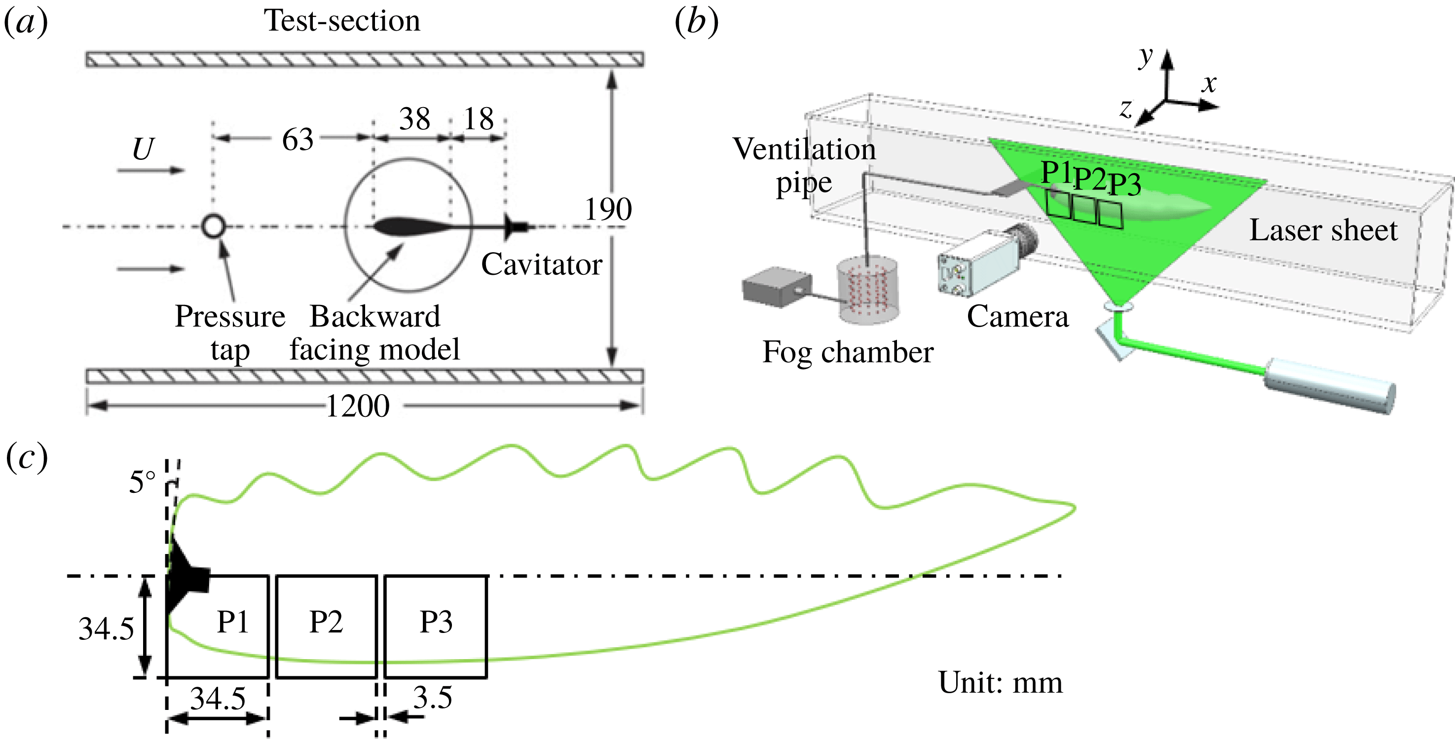
Reference Shao, Karn, Ahn, Arndt and Hong2017). As shown in figure 1(a), a backward-facing cavitator (with detailed information provided in Karn et al.
Reference Karn, Arndt and Hong2015) of 30 mm-diameter is employed to generate a free standing ventilated supercavity for the experiments. Note that ‘free standing’ here refers to the fact that the cavity does not enclose a solid object nor interact with any solid surfaces (for example, mounting struts) downstream of the cavitator. The cavitator is mounted in the downstream of a hydrofoil through an 18 mm extension tube. The hydrofoil strut has a thickness of 5 mm to minimize wake influence on the supercavity.
Schematics of (a) the test section and backward-facing cavitator, (b) the experiment setup and (c) the field of view of images used for PIV measurements.

Flow visualization and planar PIV are performed using fog tracer particles for qualitative and quantitative analysis of the internal flow. Fog particles are generated using a Rosco1700 fog machine which yields a particle diameter of
 $29\pm 8~\unicode[STIX]{x03BC}\text{m}$
. The particle diameter is determined through digital images of particles illuminated by the laser sheet outside the water tunnel, with the same setup inside the water tunnel. The image size of particles is then corrected to account for light scattering effects following Raffel, Willert & Kompenhans (Reference Raffel, Willert and Kompenhans2007). We acknowledge that the size of the fog particles measured by this method may differ from the size of actual fog particles produced immediately from the fog generator, but it corresponds directly to the particles used for the PIV calculation. As shown in figure 1(b), the fog machine feeds fog particles directly into a 42 gallon fog chamber. The chamber is then connected to a ventilation line that goes through the hydrofoil strut and the cavitator to introduce the fog particles into the supercavity. The large fog chamber, maintained at atmospheric pressure, is used to ensure consistent fog supply for flow measurements. A laser sheet of
 $1\pm 0.2$
mm thickness, generated using a Photonics DM30-527 Nd/YLF high-speed laser (
 $30~\text{mJ}~\text{pulse}^{-1}$
at 3 kHz repetition rate), is employed to illuminate the particles on the central streamwise-vertical plane (i.e.
 $x$
–
 $y$
plane, with
 $z=0$
as defined figure 1
b) of the supercavity. Note that the thickness of the laser sheet is calibrated through its digital image recorded at the same location as our measurements with a reference scale in the field of view. During the experiments, the expansion angle and the centre position of the light sheet are adjusted to observe different regions of the supercavity with different magnifications. To capture images of the internal flow fields, a Photron APX-RS high-speed camera (
 $3000~\text{frames}~\text{s}^{-1}$
with full sensor size of
 $1024\times 1024$
pixels), equipped with a Nikon macro 105 mm/f5.6 lens, is positioned perpendicular to the laser sheet. During the experiments, the laser and the camera are synchronized at 3 kHz to record images for flow visualization of the entire internal flow field (i.e. a field of view
 ${\sim}300~\text{mm}\times 100~\text{mm}$
with a pixel resolution of
 $0.4~\text{mm}~\text{pixel}^{-1}$
). For PIV measurements, a higher magnification is applied to ensure sufficient resolution to capture fog particle motion for the measurements of the internal flow field. In particular, as illustrated in figure 1(c), the PIV image is recorded at three different streamwise locations (i.e. P1, P2 and P3 in the figure), and each region has a field of view of
 $34.5~\text{mm}\times 34.5~\text{mm}$
with a pixel resolution of
 $0.03~\text{mm}~\text{pixel}^{-1}$
. The three PIV measurement regions (with a gap of 3.5 mm between adjacent regions) in total cover the bottom half of the supercavity from the cavitator to 35–40 % of the streamwise extent of the supercavity. It is worth noting that no reliable PIV images can be recorded further downstream due to the strong disturbances/distortion at the liquid–gas interface.
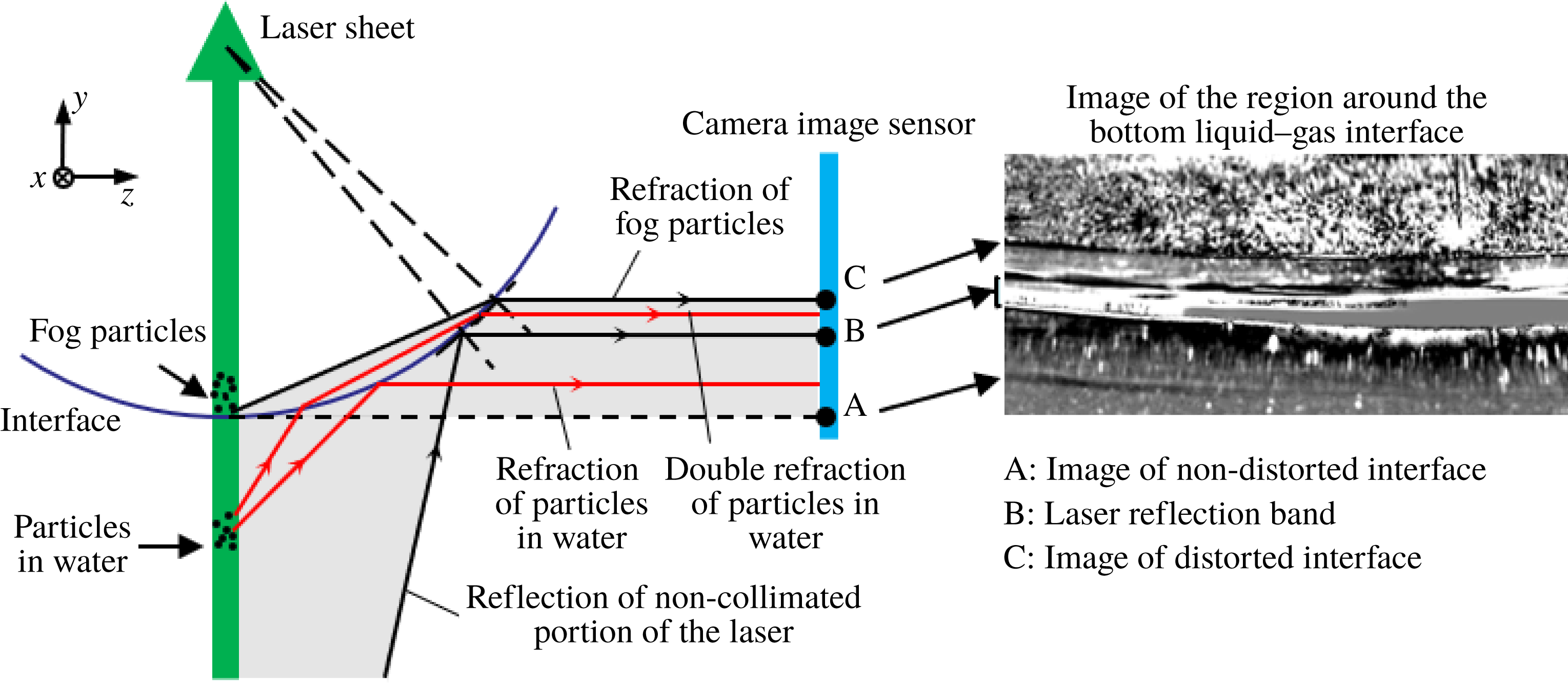
Schematic showing the distortion of the particle image due to light reflection and refraction at the liquid–gas interface of the supercavity. The shaded region shows that from location A to C, the camera image sensor only records information outside the supercavity (i.e. images of illuminated sediment particles in water and the scattered laser band), while the images of fog particles inside the supercavity are recorded above location C.

The recorded particle images are postprocessed using a modified histogram equalization algorithm developed by Roth & Katz (Reference Roth and Katz2001) to enhance the signal-to-noise ratio of particles before the PIV calculation. However, as illustrated in figure 2, these enhanced images are distorted views of the particle field inside the supercavity as the camera images through the liquid–gas interface. Specifically, the distorted particle images contain both the particles inside the supercavity (i.e. ventilated fog particles) and sediments in the water. The location A marked in figure 2 shows the real location of the liquid–gas interface, which appears as a faint dark curve in the inset image of the region around the bottom liquid–gas interface. Comparatively, the location C marks the location of the distorted liquid–gas interface, i.e. a sharp dividing line in the inset image. Due to light reflection and refraction at the interface, each particle illuminated by the laser sheet near the interface in the water forms two images within the band marked by location A and C: one from the reflection at the interface and the other from double refraction as scattered light propagates through the interface. Note that the experiments use city tap water which contains small sediments shown as particles in the images. In addition, the imperfection of the laser sheet (i.e. non-collimated low intensity portion of the laser) causes a direct reflection at the interface, corresponding to location B in the figure. The reflection results in a band of glare in the image. However, such a laser reflection band does not affect our PIV measurements of the internal flow since it does not interfere with the signals of the particle field inside the supercavity.
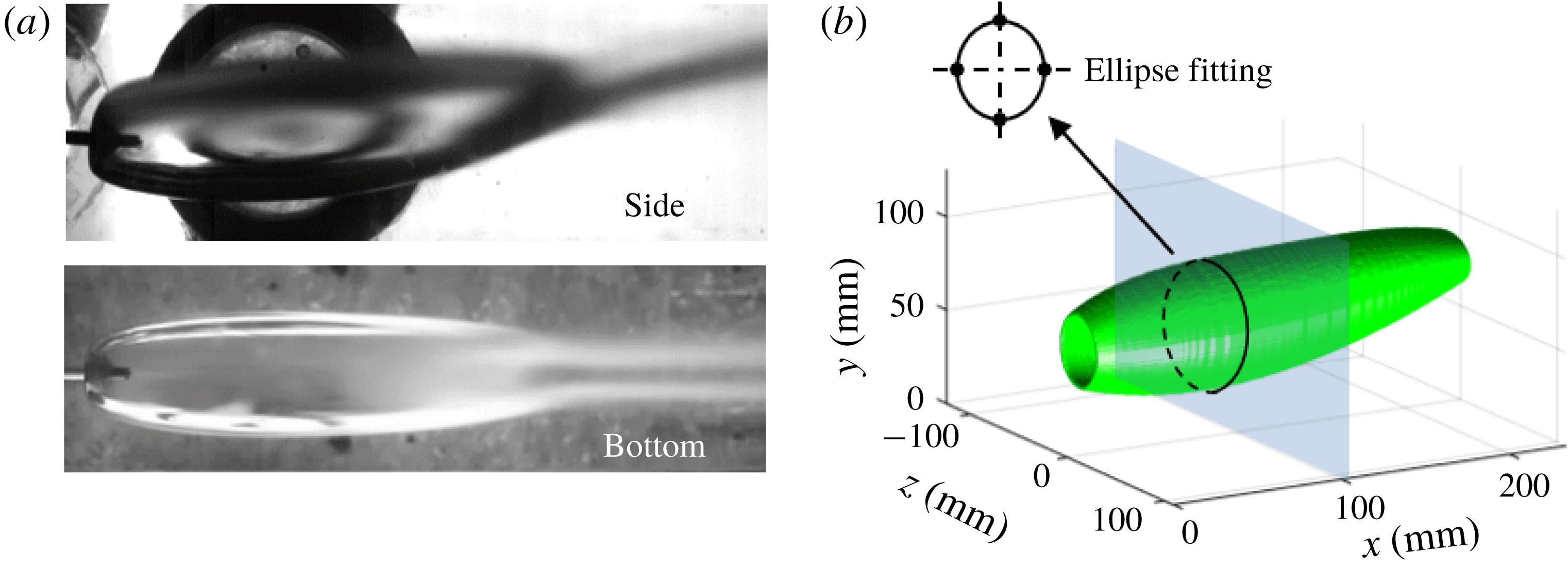
(a) Time-averaged images of the side and bottom views of the entire supercavity. (b) The 3D topology of the supercavity reconstructed from the side and bottom views shown in (a) through ellipse fitting at each cross-section.

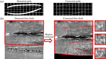
To eliminate the distortion due to imaging through the interface, the enhanced particle images are further processed using the ray tracing mapping method presented in Kumar et al. (Reference Kumar, Karn, Arndt and Hong2017). In order to implement the ray tracing mapping method, the 3D geometry of the liquid–gas interface must be obtained a priori. Such 3D geometry is obtained by imaging the supercavity from two orthogonal views, i.e. from the side and bottom of the test section. Figure 3(a) presents the time-averaged images of the supercavity from these two views. As illustrated in figure 3(b), the top, bottom and side boundaries of the cross-section of the supercavity at each streamwise location are extracted from the images and fitted with an ellipse. A sequence of these elliptical cross-sections is then combined to reconstruct the 3D surface of the supercavity. Successively, using the 3D surface as an input, the ray tracing mapping method is first validated by correcting a distorted grid pattern of known spacing, as shown in figure 4(a). Figure 4(b) presents the distorted and the distortion-corrected images of the internal flow field using the ray tracing mapping method. After the correction, the actual horizontal and vertical extents of the particle field are recovered. The close-up view of particle image samples in three interrogation windows (32 pixels × 32 pixels) are also presented in figure 4(b), where distinctive particle patterns are captured. Although these particle images deviate from the standard PIV particle images due to information loss and signal blurring caused by imaging through the liquid–gas interface, they do yield reliable velocity vectors with an average correlation factor of approximately 0.7. Note that during the PIV experiments, strong disturbances can occur on the interface and induce some vertical fringe patterns in our sample region, imposing a detrimental effect on the PIV measurements. Approximately 30 % of the recorded PIV images are strongly affected by such fringe patterns. These images have already been excluded from the PIV analysis. For the remaining images used for PIV analysis, the effect of the interface disturbance is evaluated quantitatively by tracking fluctuations of the vertical location of both the bottom and the top interfaces of the supercavity in the digital images. The maximum vertical displacement of the interface from its mean location within the streamwise span of our PIV measurements is found to be 1.2 mm at the top and 0.6 mm at the bottom. Overall, the corresponding maximum uncertainty in the grid location of PIV vectors is less than 10 % of the interrogation window size. Therefore, the uncertainty caused by interface disturbance is insignificant for the present PIV analysis. The distortion-corrected images are processed using a multipass cross-correlation from LaVision DaVis7.2 to obtain instantaneous velocity vector fields. The method applies a minimal interrogation window size of
 $32\times 32$
pixels with 75 % overlap, resulting in a vector spacing of 0.27 mm for the velocity vector fields. It is also worth noting that, as shown in the figure 4, a narrow dark band (i.e. a region of very few particles of
 ${<}1024~\text{pixels}\times 96~\text{pixels}$
) appears intermittently in the reverse flow region. The region is shown as a bright band of saturated pixels in the original particle images and becomes dark in the enhanced images after background subtraction. This band is likely to be a result of the reflection of the non-collimated portion of the laser on the side interface, resulting in spurious velocity vectors in the region after cross-correlation. Nevertheless, these spurious velocity vectors point downstream and are significantly different from the actual flow in the reverse flow region. Therefore, these vectors are filtered out during the postprocessing and then interpolated using reliable velocity data in the region.
Distorted and corrected (a) grid patterns and (b) internal particle field. The close-up view samples of the particle field (
 $32~\text{pixels}\times 32~\text{pixels}$
) in (b) are also presented to demonstrate distinct particle patterns for the PIV calculation.

Experimental conditions for the supercavities with RJ and TV closure modes.

In addition to the internal flow measurements, we also conduct pressure measurements using a hypodermic tube at the backside of the cavitator (for
 $P_{C}$
) and a pressure tap located upstream of the airfoil strut (for
 $P_{\infty }$
). These measurements are performed separately from the flow measurements, under the same flow and ventilation conditions, to obtain the corresponding cavitation number
 $\unicode[STIX]{x1D70E}$
for each test case. It is worth noting that during the experiments the angle of attack of the airfoil strut is set at
 $5\pm 0.5^{\circ }$
to ensure a relatively smooth bottom interface of the supercavity for the laser sheet to remain undisturbed as it penetrates the interface. The measurements are conducted for supercavities with two closure modes: re-entrant jet (RJ) closure and twin-vortex (TV) closure, under the flow and ventilation conditions listed in table 1. The uncertainties of
 $U_{W,\infty }$
,
 $P_{\infty }$
,
 $P_{C}$
and
 $Q_{As}$
are obtained from the corresponding instruments (the National Instrumental Data Acquisition System for
 $U_{W,\infty }$
, Rosemount pressure sensor for
 $P_{\infty }$
,
 $P_{C}$
, and Omega Flow Meter for
 $Q_{As}$
). The uncertainties of
 $Fr$
,
 $C_{Qs}$
and
 $\unicode[STIX]{x1D70E}_{C}$
are calculated based on the propagation of uncertainty. The overall uncertainty analysis of these measurements is in accordance with our previous investigations (for example, Karn et al.
Reference Karn, Arndt and Hong2015). In addition, the cavity length (
 $L$
), shown in table 1, is measured as the streamwise distance from the cavitator to the closure (marked by the onset of the two counter-rotating vortices) using 40 s digital videos with
 $0.34~\text{mm}~\text{pixel}^{-1}$
resolution from both the bottom and side views. The standard deviation of the cavity length during the whole record span 3.0 % of its mean length for the RJ case and 1.5 % for the TV case. For each closure mode, the PIV images are recorded in all three regions (i.e. P1, P2 and P3 as shown in figure 1
c). At each region, a total of four sequences of internal flow images are recorded. Each sequence contains 2048 images and corresponds to a sampling period of 0.68 s. Furthermore, to ensure statistical robustness of our mean flow measurements, the ensemble average is applied to four sequences which span a time duration of 24 min. Such a time scale (i.e. 24 min) is sufficient to ensure ergodicity of the turbulence measurement, considering the time scale corresponding to the integral time scale of our experiment is approximately 10 ms (estimated based on cavitator size divided by mean advection flow velocity).
3 Results
3.1 Flow visualization
The large field of view and close-up view near the cavitator of the internal flow patterns inside the supercavity with (a) RJ closure (supplementary movies S1 for far view, S2 for near view) and (b) TV closure (supplementary movies S3 for far view, S4 for near view). The scale bars are applied to both TV and RJ cases correspondingly.

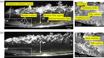
Flow visualization based on fog patterns provides a qualitative view of detailed gas flows inside the ventilated supercavity. As shown in figure 5(a), for the ventilated supercavity with RJ closure, the internal flow exhibits three main features: (i) a ventilation influence region observed behind the cavitator; (ii) a flow region of high shear extended from the liquid–gas interface (referred to as internal boundary layer); and (iii) a reverse flow region occurring in the centre of the supercavity. In addition, supplementary movies S1–S4, available at https://doi.org/10.1017/jfm.2018.1006, are provided to offer better presentation on the instantaneous flow structure inside the supercavity. Specifically, in the ventilation influence region, the air is entrained by the moving liquid–gas interface shortly after it exits the ventilation holes on the cavitator. Note that quantitative determination of the streamwise extent of the ventilation influence region is based on the mean velocity field, as will be discussed in § 3.2. Here the fog visualization only provides a qualitative description on the extent of this region, which is estimated from the cavitator to the location where the dense fog region has a minimum vertical extent. As it shows, in this region, a portion of air is entrained from the internal boundary layer to the reverse flow region and circulated back to the boundary layer. The ventilation influence region has a vertical extent close to
 $d_{C}$
, and the horizontal extent of the region (visualized by the fog pattern) fluctuates at approximately
 $2d_{C}$
downstream from the cavitator. Downstream of the ventilation influence region, the development of an internal boundary layer with appreciable air entrainment towards the interface can be clearly observed. The internal boundary layer is similar to the one developed from a moving foil that moves at the same velocity as the local water flow (Spurk Reference Spurk2002). Due to the strong disturbance caused by impingement of gas jets from the ventilation holes at the liquid–gas interface, the boundary layer transitions directly to a turbulent boundary layer. The boundary layer gradually grows thicker up to a location slightly downstream of the location of maximum supercavity diameter. Then the trend of boundary layer growth slows down as the supercavity reduces its diameter in the downstream. The presence of this internal boundary layer and its important role on air entrainment is consistent with the theory from Spurk (Reference Spurk2002), and a similar trend of boundary layer thickness variation was observed in the simulation from Kinzel et al. (Reference Kinzel, Lindau and Kunz2009). However, these prior studies did not specifically comment on the impact of the ventilation influence region on the general characteristics and the development of the boundary layer. The reverse flow region is observed throughout the entire streamwise span of the flow visualization (i.e. till
 ${\sim}80\,\%\,L$
downstream of the cavitator) in the centre portion of supercavity. Downstream of the ventilation influence region, the reverse flow covers the majority of the supercavity and travels with an almost uniform streamwise velocity, which is much slower than that of the moving liquid–gas interface. Besides, coherent spanwise vortical structures are advected upstream with a slight deformation in the reverse flow region, indicating the flow in this region is more uniform compared to that of the internal boundary layer. When the reverse flow approaches the location approximately
 $0.5d_{C}$
downstream of the cavitator, a clear deceleration is observed. It is worth noting that neither Spurk (Reference Spurk2002) nor Kinzel et al. (Reference Kinzel, Lindau and Kunz2009) indicated the presence of reverse flow for the supercavity with RJ closure even though Kinzel et al. noted such flow could occur for TV type supercavities. In addition, some subtle flow features can be observed from our flow visualization. For example, in the ventilation influence region, groups of tiny vortices with both clockwise and counter-clockwise rotation appear behind the cavitator and immediately above the liquid–gas interface, as shown from the close-up view in figure 5(a). These vortical structures are produced by ventilation jets and are likely to depend on the configuration of the ventilation schemes according to some of our preliminary tests using cavitators with modified ventilation. Moreover, at the outer extent of the internal boundary layer, a series of hairpin-like vortical structures emerge and are entrained into the reverse flow region. Note that the orientation of these coherent structures is opposite to that of the hairpin vortices observed in the wall-bounded flows due to the reversed direction of the shear stress associated with the moving liquid–gas interface.
As shown in figure 5(b), the supercavity with TV closure displays main flow features similar to those in the RJ supercavity. Specifically, the ventilation influence region has a similar vertical extent (i.e.
 ${\sim}d_{C}$
) and streamwise extent (i.e. developing from 0 to
 ${\sim}2d_{C}$
downstream of the cavitator). However, some apparent discrepancies on the detailed characteristics of the reverse flow and the internal boundary layer are observed. In particular, the reverse flow shows a wider extent, almost filling the entire lateral span of the supercavity, and moves faster in the streamwise direction. Moreover, there seems to be more occurrences of coherent vortical structures being rolled-up from the boundary layer and entrained into the reverse flow region. Additionally, as shown in the close-up view in figure 5(b), more tiny vortices with enlarged size are produced in the vicinity of the location where the ventilation jet impinges the liquid–gas interface, due to the increase in the flow rate of ventilation. Furthermore, the close-up view of the supercavity with TV closure presents a series of coherent vortices rolled-up along the shear interface between the reverse flow and the ventilation jet flow. These vortices may be induced by enhanced Kelvin–Helmholtz (KH) instability, which is caused by the increased shear rate at the shear interface.
3.2 Mean flow field
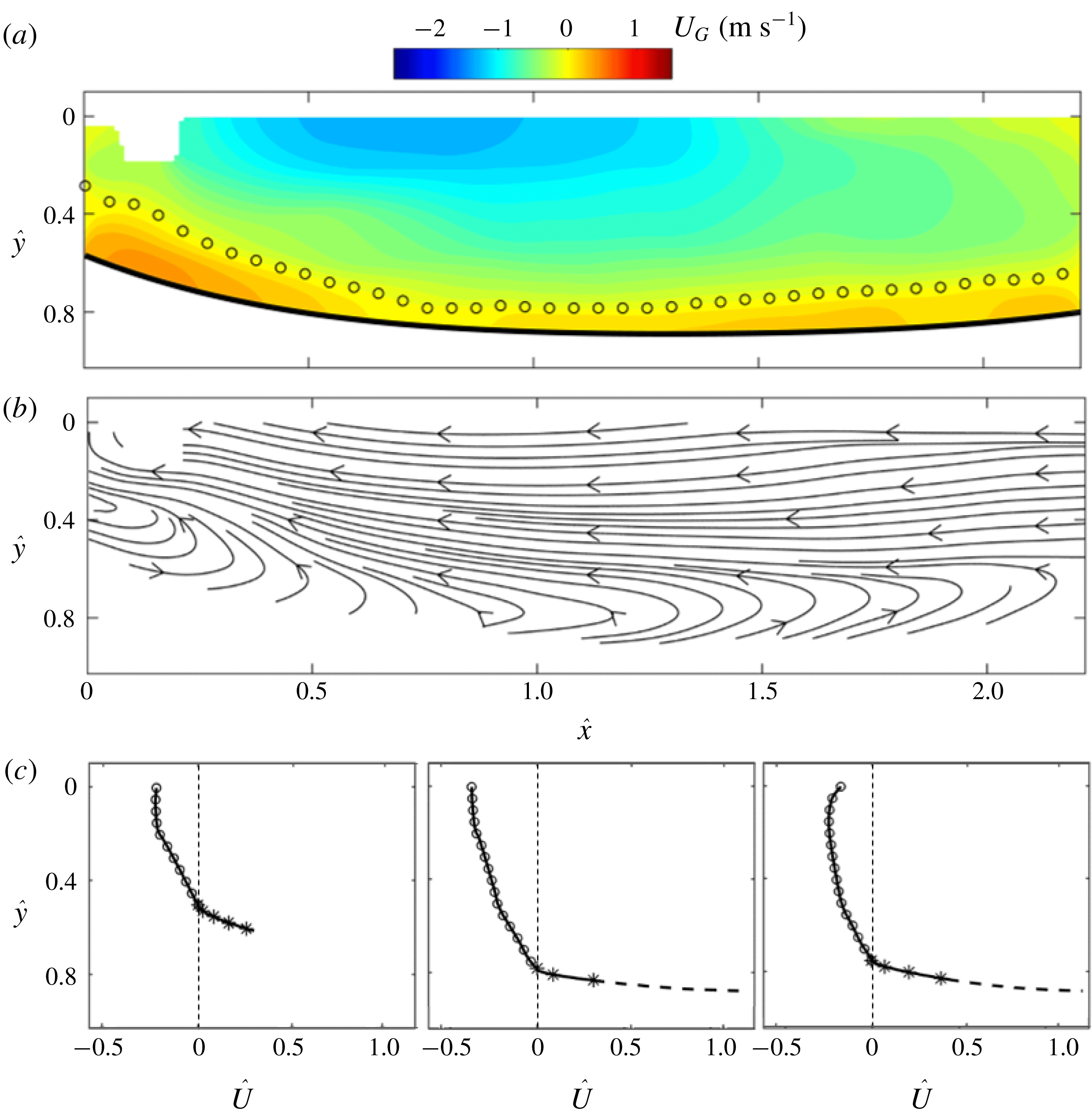
To provide quantitative characterization of the main internal flow features observed from the flow visualization, the time-averaged internal flow fields are examined for supercavities of both the RJ and TV closure modes. Figure 6 shows the mean internal flow field of the RJ supercavity obtained by compiling ensemble-averaged flow fields (after the distortion correction) measured at three streamwise locations. Note that vectors in the gaps (
 ${\sim}3.5$
mm) between adjacent PIV flow fields are interpolated based on five columns of interrogation windows (corresponding to
 ${\sim}5$
mm) on either side of each gap to ensure a smooth transition. The streamwise location (
 $x$
) and vertical location (
 $y$
) of the mean velocity field are normalized using the supercavity half-length (
 $L_{Dmax}$
), i.e. the distance from the cavitator to the location of the maximum supercavity diameter
 $D_{max}$
, and the cavitator diameter (
 $d_{C}$
), respectively (i.e.
 $\hat{x}=x/L_{Dmax}$
,
 ${\hat{y}}=y/d_{C}$
).
Ensemble-averaged (a) internal streamwise velocity contour, (b) streamlines and (c) velocity profile at
 $\hat{x}=0.25$
, 1.00, 1.75 for the supercavity with RJ closure. The bold solid curve and the open circles in (a) mark the liquid–gas interface and the locations of zero streamwise velocity, respectively. The circles and asterisks in (c) present the velocity distribution in the reverse flow and the internal boundary layer, respectively. The dashed curve in (c) presents the interpolated velocity profile close to the liquid–gas interface. Note that we do not add the interpolated segment for the velocity profile at
 $\hat{x}=0.25$
since it is situated in the ventilation influence region.

As shown in figure 6(a,b), the internal streamwise velocity field
 $U_{G}$
(the subscript ‘
 $G$
’ stands for ‘Gas’) exhibits three flow regions (the ventilation influence region, the reverse flow region and the internal boundary layer), consistent with the flow visualization results. In particular, the liquid–gas interface is extracted using a fourth-order polynomial fit and plotted as solid curve beneath the velocity field in figure 6(a). A layer of zero streamwise velocity (marked using open circles) can be determined using the mean flow field, which separates the forward flow in the developing internal boundary layer and the reverse flow in the bulk centre region of the supercavity.
The contour of mean streamwise velocity field shows the presence of the ventilation influence region behind the cavitator, consisting of a large portion of forward flow and the clear shear layer in figure 6(a). The streamwise extent of the ventilation influence region is estimated to be approximately
 $0.8L_{Dmax}$
(
 $\hat{x}\approx 0.8$
), measured from the cavitator (i.e.
 $\hat{x}=0$
) to the location where the forward flow reaches its minimum vertical extent from the interface (i.e.
 $\hat{x}\approx 0.8$
). Moreover, based on the streamline patterns of the internal flow (figure 6
b), a circulation region with a vertical extent of approximately
 $0.6d_{c}$
(estimated behind the cavitator at
 $\hat{x}\approx 0.2$
), i.e. the ventilation influence region, can be clearly observed. As shown in figure 6(a), the reverse flow covers the centre portion of the supercavity and the speed of the reverse flow first increases as it moves upstream from the closure region towards the location of
 $D_{max}$
. This trend may be associated with the streamwise adverse pressure gradient inside the supercavity, which has been shown in numerical studies of a ventilated supercavity (for example, Kirschner et al.
Reference Kirschner, Fine, Uhlman and Kring2001; Cao et al.
Reference Cao, Karn, Arndt, Wang and Hong2017; Kinzel et al.
Reference Kinzel, Krane, Kirschner and Moeny2017). Around the location of
 $D_{max}$
(i.e.
 $\hat{x}\approx 1$
), the reverse flow reaches its maximum speed of
 $1.26~\text{m}~\text{s}^{-1}$
, corresponding to 35 % of the velocity of the liquid–gas interface (
 $U_{WG}$
). The speed of the reverse flow remains relatively unchanged as it moves further upstream and decreases sharply as it approaches the cavitator (i.e.
 $\hat{x}\approx 0.5$
) due to the blockage effect of the cavitator. In comparison, the internal boundary layer, identified as the region between the location of zero velocity and the liquid–gas interface downstream of the ventilation influence region, starts with a minimum thickness of 2.2 mm at
 $\hat{x}\approx 0.8$
. The boundary layer grows thicker downstream and the trend of boundary layer growth slows down after
 $\hat{x}\approx 1.7$
. It is also worth noting that at
 $\hat{x}\approx 1.7$
, the reverse flow speed reaches its maxima at a location slightly below the centreline of the cavitator (figure 6
c). Such a pattern is consistent with a recent numerical simulation by Cao et al. (Reference Cao, Karn, Arndt, Wang and Hong2017) under similar flow conditions (i.e. 30 mm cavitator,
 $4~\text{m}~\text{s}^{-1}$
incoming flow speed and TV type closure). It is likely to be a result of the asymmetric profile of the supercavity due to the buoyancy effect at low
 $Fr$
number.
To further quantify the velocity distribution at different regions inside the supercavity, velocity profiles at three selected streamwise locations (i.e.
 $\hat{x}=0.25$
, 1.00 and 1.25) are presented in figure 6(c). The streamwise internal flow velocity
 $U_{G}$
is normalized using the velocity of the liquid–gas interface
 $U_{WG}$
(i.e.
 $\hat{U} =U_{G}/U_{WG}$
), where
 $U_{WG}$
can be derived from the equation below according to Logvinovich (Reference Logvinovich1972):
 $$\begin{eqnarray}U_{WG}(y)=\sqrt{U_{W,\infty }^{2}(1+\unicode[STIX]{x1D70E})+2gy}.\end{eqnarray}$$
In practice, in our experiments,
 $U_{W,\infty }^{2}(1+\unicode[STIX]{x1D70E})\gg 2gy$
, so we calculate
 $U_{WG}$
using
 $U_{WG}\approx U_{W,\infty }\sqrt{1+\unicode[STIX]{x1D70E}}$
, and use it to scale the internal flow velocity. The normalized velocity distribution of the reverse flow and the internal boundary layer are marked using circles and asterisks, respectively. Moreover, note that due to size limits in the interrogation window size for PIV, there is a region of
 ${\sim}1$
mm immediately above the liquid–gas interface where the velocity cannot be accurately resolved. Therefore, we interpolate the velocity profile in this region (outside the ventilation influence region) using the turbulent boundary layer model presented in Spurk (Reference Spurk2002). Specifically, according to the model, the streamwise velocity
 $U_{G}(r)$
at a location at distance
 $r$
from the liquid–gas interface (inside the boundary layer) is calculated using the following equation:
 $$\begin{eqnarray}\frac{U_{G}(r)}{U_{\unicode[STIX]{x1D70F}}}=\frac{U_{WG}}{U_{\unicode[STIX]{x1D70F}}}-\left[\frac{1}{\unicode[STIX]{x1D705}}\ln \left(\frac{rU_{\unicode[STIX]{x1D70F}}}{\unicode[STIX]{x1D708}}\right)+2\frac{\unicode[STIX]{x1D6F1}}{\unicode[STIX]{x1D705}}\sin ^{2}\left(\frac{\unicode[STIX]{x03C0}r}{2\unicode[STIX]{x1D6FF}}\right)+B\right],\end{eqnarray}$$
where
 $\unicode[STIX]{x1D708}$
is the kinematic viscosity of the air (
 $1.5\times 10^{-5}~\text{m}^{2}~\text{s}^{-1}$
),
 $\unicode[STIX]{x1D705}$
the Karman constant (0.41),
 $\unicode[STIX]{x1D6F1}$
and
 $B$
are empirical values (0.55 and 5) based on the empirical results provided in Schlichting et al. (Reference Schlichting, Gersten, Krause and Qertel1955),
 $\unicode[STIX]{x1D6FF}$
the measured thickness of the internal boundary layer, and
 $U_{\unicode[STIX]{x1D70F}}$
the friction velocity calculated using the interface condition (Spurk Reference Spurk2002):
 $$\begin{eqnarray}0=\frac{U_{WG}}{U_{\unicode[STIX]{x1D70F}}}-\left[\frac{1}{\unicode[STIX]{x1D705}}\ln \left(\frac{\unicode[STIX]{x1D6FF}U_{\unicode[STIX]{x1D70F}}}{\unicode[STIX]{x1D708}}\right)+2\frac{\unicode[STIX]{x1D6F1}}{\unicode[STIX]{x1D705}}+B\right].\end{eqnarray}$$
In general, the velocity profiles show consistent trends regarding the development of the reverse flow region and the internal boundary layer. Specifically, immediately behind the cavitator (i.e. at
 $\hat{x}=0.25$
), the reverse flow covers the smallest vertical span (
 $0.5d_{C}$
) in comparison with other streamwise locations. The primary reason is the effect of the forward flow induced by ventilation jet flow in a relatively narrow cross-section of the cavity. As the cavity increases its diameter, the reverse flow increases its span to approximately
 $0.8d_{C}$
at
 $\hat{x}=1.00$
with an appreciable increase of flow speed. Further downstream (for example, at
 $\hat{x}=1.75$
), the reverse flow occupies a slightly smaller region (approximately
 $0.75d_{C}$
) with a reduced magnitude. For all locations, the forward flow occupies a significantly smaller region compared to the reverse flow.
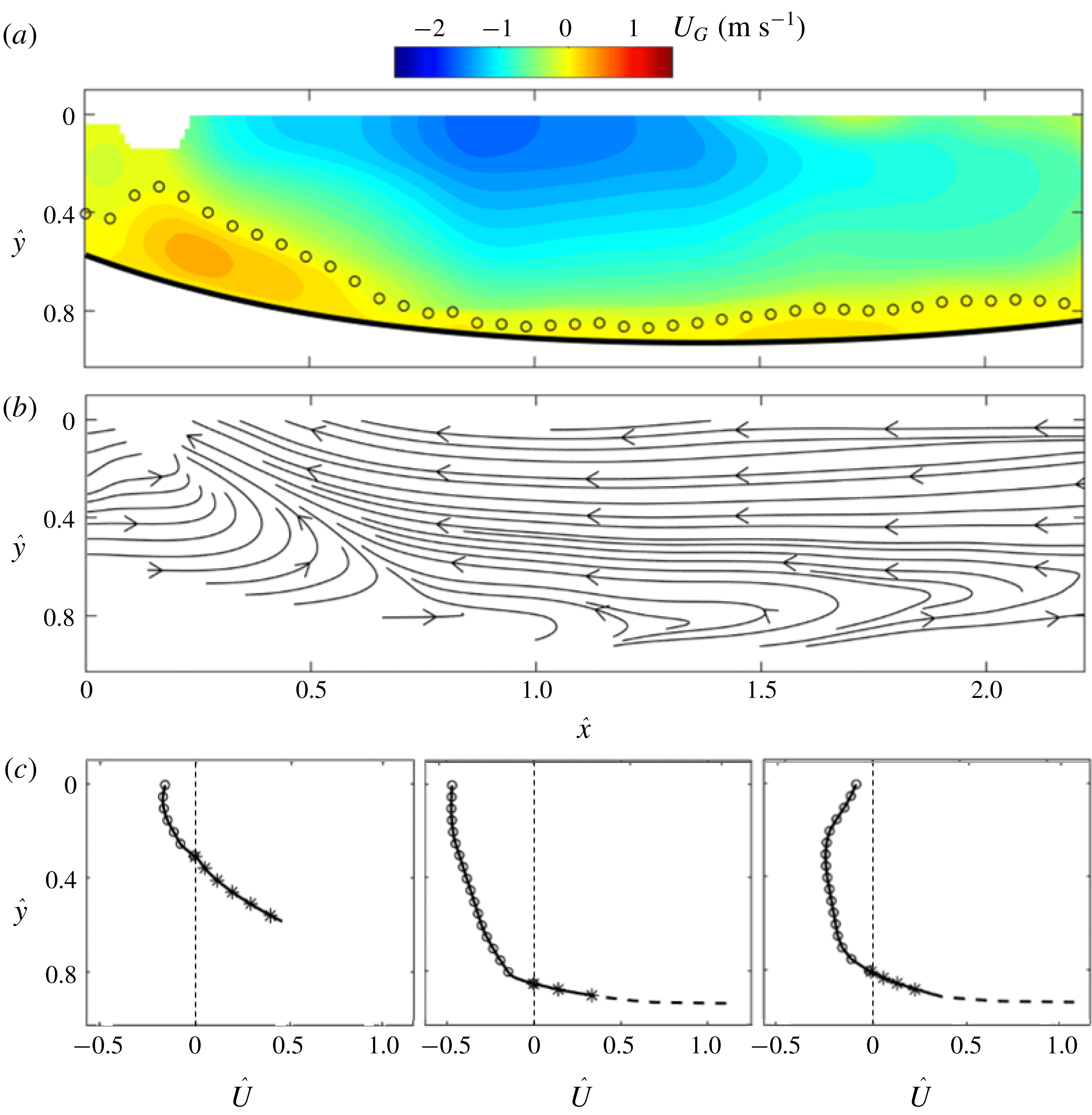
Ensemble-averaged (a) internal streamwise velocity contour, (b) streamlines and (c) velocity profile at
 $\hat{x}=0.25$
, 1.00, 1.75 for the supercavity with TV closure. The symbols follow the same convention as those in the figure 6.

In comparison with figure 6, figure 7 shows the mean internal flow field of the TV supercavity. Compared with the flow conditions of the RJ supercavity, as shown in table 1, the TV supercavity is formed using the same cavitator with the same
 $Fr$
but increased
 $Q_{As}$
. Under such conditions, the half-length of the TV supercavity stays unchanged, consistent with a number of prior studies (for example, Logvinovich Reference Logvinovich1972; Epshtein Reference Epshtein1973; Shao et al.
Reference Shao, Karn, Ahn, Arndt and Hong2017). Therefore, the streamwise location (
 $x$
) and vertical location (
 $y$
) of mean velocity can still be normalized by the same supercavity half-length (
 $L_{Dmax}$
) and cavitator diameter (
 $d_{C}$
), respectively. As shown in figure 7(a), the contour of the internal streamwise velocity field for the TV supercavity exhibits similar characteristics for the ventilation influence region, the reverse flow region and the internal boundary layer compared to the RJ supercavity. Specifically, the streamwise extent of the ventilation influence region stays approximately the same as that of the RJ supercavity. The trends in development of the reverse flow velocity and the internal boundary layer thickness in the streamwise direction are also similar. However, are still appreciable discrepancies in the flow regions. First, the ventilation influence region has an expanded vertical extent of approximately
 $0.8d_{C}$
(compared with
 $0.6d_{C}$
in the RJ case) as estimated from the streamline distribution shown in figure 7(b). The vertical expansion is also illustrated by comparing the velocity profile measured at
 $\hat{x}=0.25$
in figure 7(c) with that in figure 6(c). The vertical expansion of the ventilation influence region may be attributed to the presence of stronger ventilation jet flow in the TV case. Second, the magnitude of the reverse flow shows an approximately 20 % increase with respect to that in the RJ case, potentially due to a larger adverse pressure gradient. Such an increase is also evidenced more clearly by comparing the velocity profile measured at
 $\hat{x}=1.00$
in figure 7(c) with that in figure 6(c). Third, the internal boundary layer becomes thinner along the liquid–gas interface in the TV case. Comparing to the RJ case (figure 6
c), the reverse flow also shows a decaying strength towards the centreline of the cavity (figure 7
c) with similar causes as discussed previously (i.e. the asymmetric cavity profile).
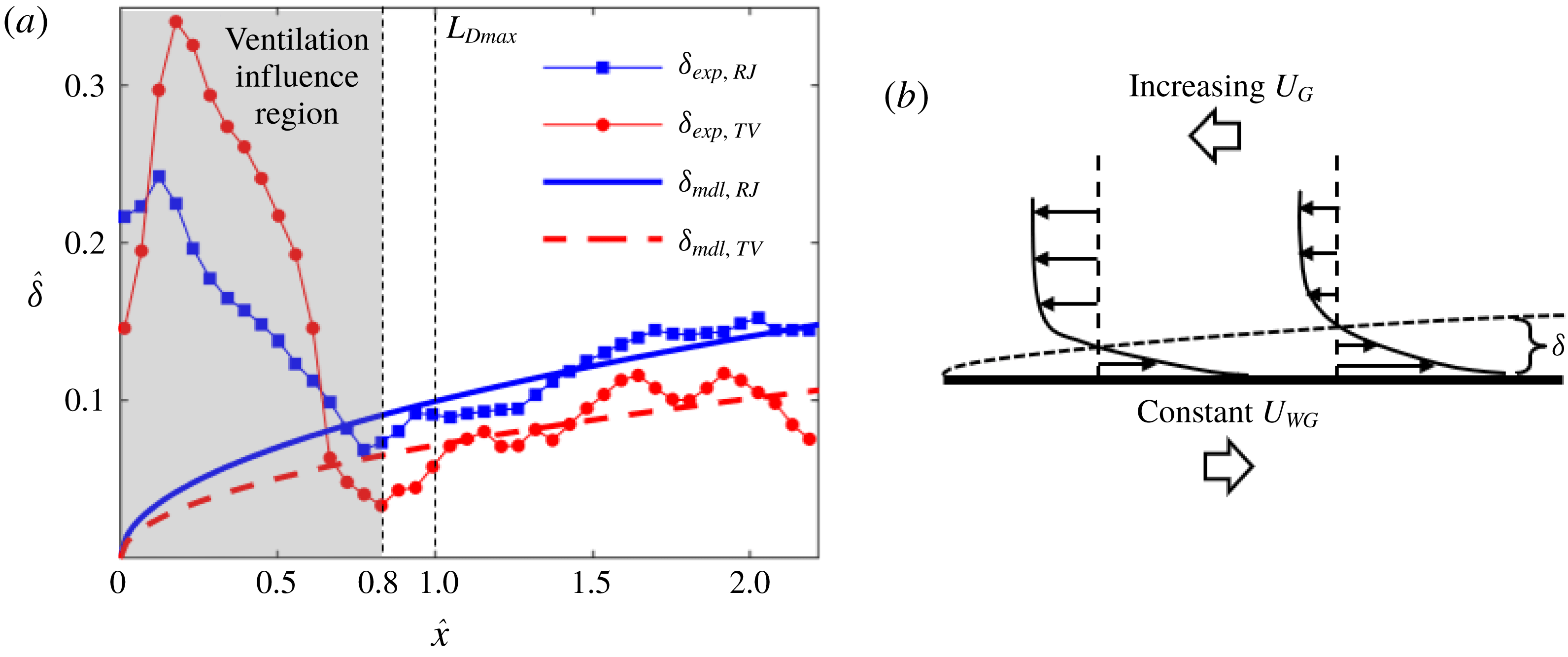
(a) Comparison of measured and modelled internal boundary layer thickness of the RJ and TV supercavities with respect to the streamwise location. (b) Schematic of a boundary layer formed on a moving plate with an external flow moving in the opposite direction.

Furthermore, the variation of the internal boundary layer thickness is quantified and compared between the RJ and TV cases based on the results shown in figures 6 and 7. As mentioned earlier, the boundary layer thickness in our current flow setting is defined as the distance between the liquid–gas interface and the location of zero streamwise velocity at each streamwise location. Figure 8(a) shows the variation of boundary layer thickness along the interface. The thickness
 $\unicode[STIX]{x1D6FF}$
is normalized by the cavitator diameter
 $d_{C}$
(i.e.
 $\hat{\unicode[STIX]{x1D6FF}}=\unicode[STIX]{x1D6FF}/d_{C}$
). Note that the scaled vertical extent of the forward moving flow in the ventilation influence region (i.e.
 $\hat{x}\approx 0.8$
) is defined in the same way as that of the internal boundary layer and plotted in figure 8(a) for comparison. For the RJ supercavity, the experimentally measured thickness (
 $\unicode[STIX]{x1D6FF}_{exp,RJ}$
) shows that the internal boundary layer starts at
 $\hat{x}\approx 0.8$
with a minimum thickness of
 ${\sim}0.07d_{C}$
. The boundary layer gradually grows thicker along with the interface. The increasing trend starts to slow down at
 $\hat{x}\approx 1.7$
due to the increase of adverse pressure gradient in the streamwise direction as the closure is approached, and the boundary layer reaches the maximum thickness of
 ${\sim}0.15d_{C}$
at
 $\hat{x}\approx 2$
. Note that the measured thickness shows some jitter along the interface which may be caused by the uncertainties involved in determining the interface and convergence of the mean flow field. In comparison, the internal boundary layer thickness of the TV supercavity (
 $\unicode[STIX]{x1D6FF}_{exp,TV}$
) starts at approximately the same streamwise location (i.e.
 $\hat{x}\approx 0.8$
), but with a smaller magnitude of
 ${\sim}0.04d_{C}$
. Along with the interface
 $\unicode[STIX]{x1D6FF}_{exp,TV}$
develops in a similar way to
 $\unicode[STIX]{x1D6FF}_{exp,RJ}$
. Over all measured locations,
 $\unicode[STIX]{x1D6FF}_{exp,TV}$
is approximately 20 % smaller than
 $\unicode[STIX]{x1D6FF}_{exp,RJ}$
in an average sense.
To further understand the internal boundary layer growth, a theoretical calculation is proposed to estimate the boundary layer thickness. As illustrated in figure 8(b), after exiting the ventilation influence region (i.e.
 $\hat{x}>0.8$
), the internal boundary layer is approximated as a boundary layer developed over a moving plate with an external flow moving in the opposite direction. Under this setting, the shear stresses from the liquid and gas sides at the liquid–gas interface need to be balanced and it should be noted that the dynamic viscosity of the water is significantly higher than that of the air. As a result, the velocity gradient normal to the boundary layer on the water side (referred to as external boundary layer) is negligible compared with that of the internal boundary layer. Under such conditions, according to Spurk (Reference Spurk2002), the liquid–gas interface can be regarded as a plate moving at the same velocity (
 $U_{WG}$
) as the free-stream velocity of water at the corresponding streamwise location. As mentioned above,
 $U_{WG}$
is approximately constant (
 ${U_{WG}\approx U}_{W,\infty }\sqrt{1+\unicode[STIX]{x1D70E}}$
, since
 $U_{W,\infty }^{2}(1+\unicode[STIX]{x1D70E})\gg 2gy$
), while the reverse internal flow gradually accelerates upstream from
 $\hat{x}\approx 2.3$
to
 $\hat{x}\approx 0.8$
, as shown in the velocity contour in figures 6(a) and 7(a). To our best knowledge, there is no established theoretical model to quantify the boundary layer thickness under such specific conditions. Therefore, we provide a simplified model to estimate the boundary layer thickness at different streamwise locations. According to the numerical simulations of ventilated supercavitation (Kirschner et al.
Reference Kirschner, Fine, Uhlman and Kring2001; Cao et al.
Reference Cao, Karn, Arndt, Wang and Hong2017; Kinzel et al.
Reference Kinzel, Krane, Kirschner and Moeny2017), the adverse pressure gradient in the domain of our PIV measurement of the internal boundary layer thickness (i.e.
 $0.8\lesssim \hat{x}\lesssim 2.3$
) is substantially smaller than that near the closure region. Therefore, we do not consider the pressure term in the control equation of the boundary layer. For laminar flow, the control equation is simplified to the well-known Blasius equation:
 $$\begin{eqnarray}f^{\prime \prime \prime }(\unicode[STIX]{x1D702})+f^{\prime \prime }(\unicode[STIX]{x1D702})f(\unicode[STIX]{x1D702})=0,\end{eqnarray}$$
where
 $\unicode[STIX]{x1D702}=y\sqrt{U_{WG}/2\unicode[STIX]{x1D708}x}$
,
 $f^{\prime }(\unicode[STIX]{x1D702})=-U_{G}(\unicode[STIX]{x1D702})/U_{WG}$
. The boundary conditions are specified as follows:
 $f(0)=0$
due to no penetration from the interface;
 $f^{\prime }(0)=1$
since the air flow has the same velocity as the interface at
 $\unicode[STIX]{x1D702}=0$
according to our discussion above;
 $f^{\prime }(\infty )=-\overline{U_{G,\infty }}/U_{WG}$
, indicating that the flow reaches the velocity of free stream (
 $\overline{U_{G,\infty }}$
) outside the boundary layer. In our calculation, the velocity of free stream
 $\overline{U_{G,\infty }}$
(
 $0.7~\text{m}~\text{s}^{-1}$
for the RJ supercavity and
 $1.1~\text{m}~\text{s}^{-1}$
for the TV supercavity) is obtained by averaging the streamwise velocity of the reverse flow measured at
 ${\hat{y}}=0$
and
 $0.8\leqslant \hat{x}\leqslant 2.3$
. Equation (3.4) can be solved using the shooting method introduced in Cebeci & Bradshaw (Reference Cebeci and Bradshaw2012), and the boundary layer thickness can be calculated using the following equation:
 $$\begin{eqnarray}\unicode[STIX]{x1D6FF}_{cal}=\sqrt{\frac{2\unicode[STIX]{x1D708}x}{U_{WG}}}\unicode[STIX]{x1D702}_{0},\end{eqnarray}$$
where
 $\unicode[STIX]{x1D702}_{0}$
is similarity variable representing the non-dimensionalized distance from the liquid–gas interface to the location of zero velocity, which is determined from
 $f^{\prime }(\unicode[STIX]{x1D702}_{0})=0$
by solving (3.4). Due to different values of
 $f^{\prime }(\infty )$
,
 $\unicode[STIX]{x1D702}_{0}$
is calculated to be 4.7 for the RJ supercavity and 3.4 for the TV supercavity. Based on (3.5), the modelled boundary layer thicknesses of the RJ and TV cavities are presented in figure 8(a) as solid and dashed curves, respectively. It is clearly observed that the modelled boundary layer thickness of the supercavity TV supercavity is thinner than that of the RJ supercavity at all locations. Compared to the experimental results, the modelled thickness in general shows a good match of the growth trend and magnitude. However, it is noticeable that the measured thickness grows more rapidly compared to the modelled thickness due to the laminar flow assumption used in the model. It is worth noting that for the flat plate the thickness of a turbulent boundary layer
 $\unicode[STIX]{x1D6FF}$
grows proportional to
 $x^{0.8}$
in the range of our Reynolds number, which aligns better with the growth rate observed in our measurements. However, no empirical model for the turbulent boundary layer can be derived under our flow settings. In addition, figure 8(a) shows experimental values are first below and then above the modelled values as the boundary layer grows downstream in the range
 $0.8\leqslant \hat{x}\leqslant 2.3$
. A possible cause of such a difference is the assumption of the constant free-stream velocity of
 $\overline{U_{G,\infty }}$
, which is below the local
 $U_{G,\infty }$
in the range
 $0.8\leqslant \hat{x}\lesssim 1.5$
and above in the range
 $1.5\lesssim \hat{x}\leqslant 2.3$
. Another cause of the difference between the experiment and the model can come from the fact that 3D effects on the boundary layer thickness are not included in our model. Nevertheless, such effects are estimated to be small considering the significant difference between the local radius of curvature of the interface and the internal boundary layer thickness in our measurement range. In the ventilation influence region (i.e.
 $\hat{x}<0.8$
), the vertical extent of the forward moving flow of both the RJ and TV cases measured from the experiment is significantly larger compared with the modelled values, due to the strong influence of the ventilation jets.
(a) Schematic showing the estimate of gas flow circulation in the reverse flow region at the bottom half of the supercavity based on the axisymmetric assumption. The estimated change of the reverse flow (
 $Q_{REV}$
) compared with the ventilation input (
 $Q_{V}$
) for the supercavity with (b) RJ and (c) TV closure.

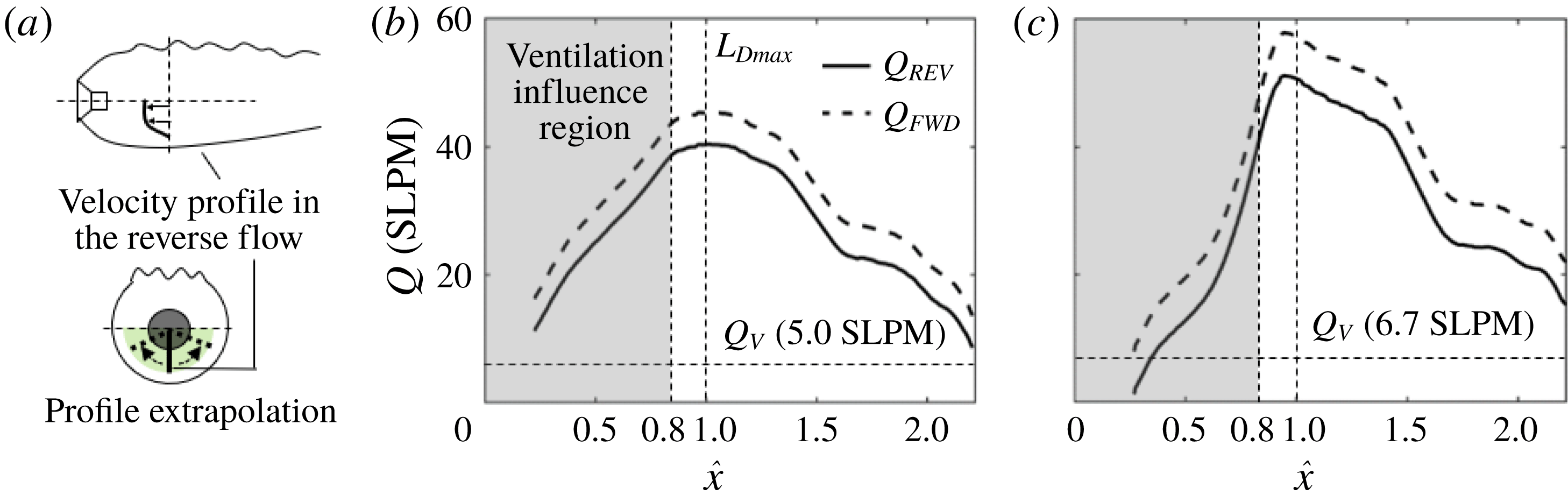
Using the internal velocity fields, we further estimate variation of the gas flow rate at each cross-section along the streamwise direction in the reverse flow region to investigate the overall gas circulation in the supercavity. As a first step, the gas flow rates obtained from the 2D plane is employed to approximate the volumetric flow rate based on the axisymmetric assumption. Specifically, as illustrated in figure 9(a), the velocity profile at each streamwise location is extrapolated axisymmetrically in the circumferential direction to cover the entire lower half of the supercavity cross-section (marked as green shaded region). Here the lower half of the cross-sections can be treated as semicircles, since ellipse fitting (introduced in figure 3) shows that the axial ratio of the cross-sections is less than 1.05 for all streamwise locations in the PIV measurement domain. After the extrapolation, the flow rates of the reverse flow (i.e.
 $Q_{REV}$
) of the half-supercavity are calculated separately at each streamwise location by integrating the velocity profile at the corresponding range of the vertical span. It is important to note that in the current study we do not estimate the gas flow rate in the internal boundary layer using the same approach above, due to the large uncertainty involved in such an estimate for the boundary layer flow. Such a large uncertainty is associated with the unresolved velocity profile near the interface and the substantial deviation from axisymmetry in the boundary layer caused by the disturbed upper interface. Instead, the gas flow rate moving forward (
 $Q_{FWD}$
) is inferred from the estimate of
 $Q_{REV}$
based on mass conservation, i.e.
 $Q_{FWD}=Q_{V}+Q_{REV}$
, where
 $Q_{V}$
is the ventilation input (estimated to be half of the overall input
 $Q_{As}$
). Note that all the volume flow rates (i.e.
 $Q_{FWD}$
,
 $Q_{REV}$
and
 $Q_{V}$
) are corrected to standard pressure and temperature, i.e. 100 kPa and 273.15 K, and calculated in the units of standard litres per minute (SLPM). Therefore, their values correspond directly to mass flow rates.
For the RJ supercavity, as shown in figure 9(b), it is evident that
 $Q_{REV}$
is significantly larger than
 $Q_{V}$
at almost all the streamwise locations. At locations of
 $\hat{x}>1$
,
 $Q_{REV}$
increases rapidly as the reverse flow moves upstream, and reaches its maximum near the location of maximum cavity diameter at
 $\hat{x}=1$
. At upstream locations of
 $\hat{x}<1$
, the reverse flow rate reduces, with gas partially dispersing into the region near the interface. Correspondingly,
 $Q_{FWD}$
shows the same trend as that of
 $Q_{REV}$
. For the TV supercavity,
 $Q_{FWD}$
and
 $Q_{REV}$
vary along the streamwise direction in the same fashion as for RJ supercavity, as shown in figure 9(c). However,
 $Q_{FWD}$
and
 $Q_{REV}$
of the TV supercavity experience a steeper change at the ventilation influence region (i.e.
 $\hat{x}<0.8$
) due to the stronger ventilation jet.
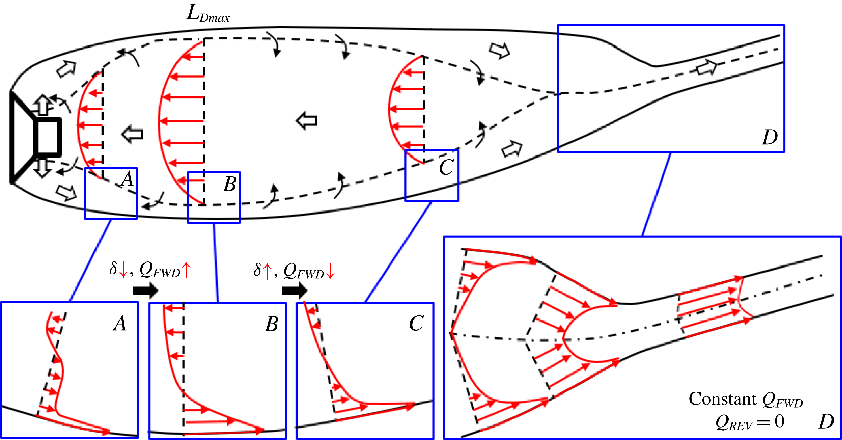
Based on the trends of gas flow rates in the internal boundary layer and reverse flow region presented above, the general picture (common for both RJ and TV supercavities) of the internal gas circulation is depicted in figure 10. Starting from the backside of the cavitator, the ventilation jet impinges directly on the liquid–gas interface as it comes out of the ventilation holes. The jet flow first experiences significant expansion and deceleration as it moves downstream, occupying a large vertical extent between the reverse flow and the liquid–gas interface. Meanwhile, the gas flow that impinges the liquid–gas interface is partially dragged downstream by the moving interface. However, in the ventilation influence region, the amount of ventilation input exceeds the entrainment capability of the moving interface, so the majority of the jet flow is not affected by the interface in this region. As illustrated in the velocity profile of region
 $A$
cropped from figure 10, in the majority of the vertical extent of the forward flow, the velocity is very low, and only a small portion of forward flow is influenced by the moving interface. As the interface moves further downstream, more ventilation gas is accelerated by the interface, and at the same time the gas is entrained from the reverse flow region towards the interface. Such an exchange of momentum between the flow near the interface and the reverse flows causes the mass flow rate of the forward flow to increase with a decreasing vertical extent.
Schematic of gas flows inside the supercavity. The gas exchange between the internal boundary layer and the reverse flow is marked with black arrows.

Outside the ventilation influence region, an internal boundary layer with a velocity profile matching that developed from a moving plate is formed, as illustrated in the region
 $B$
of figure 10. In particular, starting at the location of maximum cavity diameter (
 $L_{Dmax}$
), the gas within the internal boundary layer is stripped out and entrained by the reverse flow due to the adverse pressure gradient. Associated with the change of velocity profiles (comparing the velocity profiles between regions
 $B$
and
 $C$
of figure 10), although the gas entrained inside the internal boundary layer decreases, the boundary layer still thickens according to the trend of a boundary layer on a moving plate. Near the closure region (region
 $D$
in figure 10), the internal boundary layer merges from the upper and lower interfaces (more precisely, from all circumferential locations at the 3D interface) according to Savchenko & Savchenko (Reference Savchenko and Savchenko2012). In this region, reverse flow vanishes, and the flow of internal boundary layer increases its velocity as it moves towards the closure due to the decreasing cavity diameter. The supercavity eventually converges and a hydrodynamic wake is formed, in which the gas moves with approximately the same velocity. Due to mass conservation, in this region, the flow rate of the merged boundary layer (i.e.
 $Q_{FWD}$
) remains constant and is equal to the ventilation input
 $Q_{As}$
at all streamwise locations.
Moving upstream from the closure region, as mentioned above, the reverse flow starts at the streamwise location where the internal boundary layer merges. It is driven by the adverse pressure gradient and accelerates as it moves upstream. Besides, the vertical extent of the reverse flow also increases, according to the analysis of Riley & Weidman (Reference Riley and Weidman1989) and Ishak, Nazar & Pop (Reference Ishak, Nazar and Pop2007) for similar flow settings. Specifically, Riley & Weidman (Reference Riley and Weidman1989) and Ishak et al. (Reference Ishak, Nazar and Pop2007) study the boundary layer developed over a stretching plate and a moving wedge, respectively, both with an accelerating external flow in the opposite direction. The flow conditions in their studies share common features as ours (for example, the moving surface, the accelerating reverse flow and the adverse pressure gradient). By performing theoretical calculations based on the Falkner–Skan boundary layer model, they obtained the similarity solution for the flow velocity profile at different streamwise location. The similarity solution shows that the vertical extent of the reverse flow region widens in proportion to its developing length with a power index of
 $(1-m)/2$
, where
 $m$
(
 ${<}1$
) is a function of the adverse pressure gradient. From the closure region to the location of maximum cavity diameter (
 $L_{Dmax}$
), the reverse flow continuously entrains gas from the internal boundary layer, and the flow rate increases gradually to its maximum at
 $x=L_{Dmax}$
. From
 $x=L_{Dmax}$
to the cavitator, the adverse pressure gradient becomes negligible. Instead, the effect of cavitator blockage and the viscous shear stress associated with a sharp velocity gradient across the reverse flow and ventilation jet regions kick in, reducing the bulk velocity of the reverse flow. In addition, due to the reduction of supercavity diameter and the increase of vertical extent of the forward flow in this region, the reverse flow region narrows down its span and the reverse flow rate drops sharply.
It is worth noting that although the physical picture described above shares some similar insights to those of mechanisms portrayed in prior studies by Spurk (Reference Spurk2002) and Kinzel et al. (Reference Kinzel, Lindau and Kunz2009), some remarkable differences are presented here. Specifically, neither Spurk (Reference Spurk2002) nor Kinzel et al. (Reference Kinzel, Lindau and Kunz2009) consider the air entrainment to be affected by the ventilation jet in the ventilation influence region. Moreover, Spurk (Reference Spurk2002) claims that no reverse flow occurs in the supercavity, and the internal boundary layer keeps entraining gas until the closure region is reached. In contrast, we observe the clear presence of reverse flow and of gas in the boundary layer entrained by reverse flow after the location of maximum diameter. Although the model proposed by Kinzel et al. (Reference Kinzel, Lindau and Kunz2009) takes into account the gas exchange between the internal boundary layer and the reverse flow, they claim that the reverse flow only exists for the TV supercavity and vanishes for the RJ case. However, we observe the presence of reverse flow for both the TV and RJ cavities. In addition, the model from Kinzel et al. does not incorporate the velocity change of the reverse flow along the streamwise location, which is clearly observed from our measurements.
3.3 Gas leakage mechanism and closure modes
In this section, we will investigate the connection of the internal supercavity flow with the gas leakage mechanism and the closure modes of a ventilated supercavity. Using the physical insights gained from the internal flow investigation in §§ 3.1 and 3.2, we will explain the growth of supercavity length and the closure mode transition (i.e. from RJ to TV) as the ventilation input increases. First, we will provide new insights into the physical mechanism that contributes to the formation of RJ closure, in addition to the explanation provided in the prior studies. Then we will discuss in detail the influence of the gas leakage mechanism on the cavity growth and closure transition.
(a) Time-averaged supercavity profile at the critical point where the visible stable RJ closure is observed with the external boundary layer and the incline angle marked. (b) Schematic showing separation of the external boundary layer on a moving interface (adapted from Sears & Telionis Reference Sears and Telionis1975). (c) Visualization of water flow near the RJ closure. The trajectories of particles in water show they move towards the liquid–gas interface (please refer to the supplementary video S5 for more details).

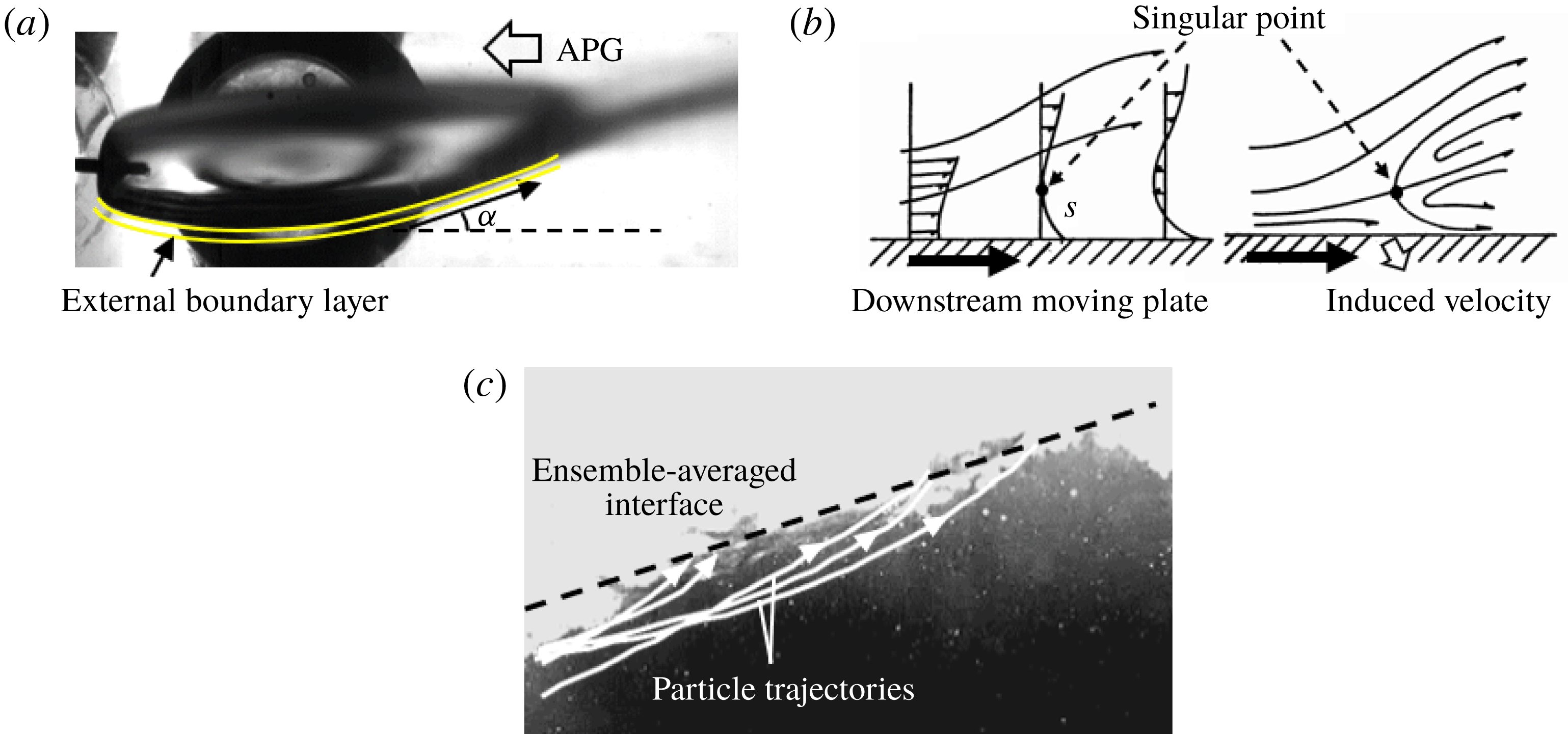
The mechanism that governs the formation of RJ closure of a ventilated supercavity has been addressed by a number of prior studies (for example, Semenenko Reference Semenenko2001; Spurk Reference Spurk2002; Savchenko & Savchenko Reference Savchenko and Savchenko2012). These studies claim that the RJ closure is formed when the water penetrates the liquid–gas interface and rolls up boundary layer material (i.e. water/air mixture) into a toroidal vortex. Specifically, Semenenko (Reference Semenenko2001) pointed out that the toroidal vortex is formed due to the collisions of fluid particles at closure. As it grows larger, the toroidal vortex is ejected from the supercavity when the friction force on the liquid–gas interface becomes equal to the re-entrant momentum. Spurk (Reference Spurk2002) stated that the small radius of curvature of the liquid–gas interface along with the reversed water flow at the closure region may contribute to the formation of the toroidal vortex, though he did not mention how the reversed water flow is formed. As more water flows into the vortex, the density of the toroidal vortex increases and the local cavitation number becomes negative, causing the vortex to be shed off from the supercavity. Savchenko & Savchenko (Reference Savchenko and Savchenko2012) suggested that Helmholtz–Taylor type mechanisms of instability cause the liquid–gas interface to become unstable, and the gas that fills the defects of the disturbed interface causes splashes at the closure region, which eventually leads to the RJ closure. However, the prior studies provided no detailed explanation of the mechanism that governs the penetration of water flow into the supercavity. Here we use flow visualization, presented in figure 11(a), to offer some further insights into such a mechanism. The supercavity geometry shown in the figure is obtained by averaging the instantaneous supercavity images recorded under 125 f.p.s. and a period of
 ${\sim}40$
s. From the figure, we notice that the re-entrant jet in this case only appears at the bottom surface of the supercavity, and the inclined angle of the cavity bottom surface (
 $\unicode[STIX]{x1D6FC}$
) is significantly larger than that of the top surface. These observations indicate the water flow close to the interface experiences a stronger adverse pressure gradient at the bottom surface. According to prior theoretical work by Stewartson (Reference Stewartson1954) and Schlichting et al. (Reference Schlichting, Gersten, Krause and Qertel1955), for 2D flow on a fixed wedge which is expanded under an adverse pressure gradient, the expansion angle (corresponding to
 $\unicode[STIX]{x1D6FC}$
in our study) has a critical value of
 $17.9^{\circ }$
. Above the critical expansion angle, flow separation occurs at downstream locations. In our experimental results, shown in figure 11(a), the inclined angle of the bottom surface (
 $\unicode[STIX]{x1D6FC}$
) measured from the 2D profile of the RJ supercavity at the critical closure transition point is
 ${\sim}18^{\circ }$
, very close to the critical angle from the theoretical work on wedge flow. Consequently, though differences between the two flows are recognized, we would like to attribute the water penetration and the formation of the RJ closure to the flow separation of the boundary layer at the water side (i.e. external boundary layer) caused by the strong adverse pressure gradient. The flow separation of a boundary layer on a moving interface has been thoroughly investigated, and a so-called Moore–Rott–Sears (MRS) criterion (co-established by Rott Reference Rott1956; Moore Reference Moore1958; Sears & Telionis Reference Sears and Telionis1975) has been proposed to explain the flow separation. This criterion is illustrated in figure 11(b), a schematic adapted from Sears & Telionis (Reference Sears and Telionis1975), showing the separation of the boundary layer on a downward moving wall (i.e. the interface moves in the same direction as the free stream). The MRS criterion claims that due to the influence of a large adverse pressure gradient, at a certain location downstream, a singular point should exist inside the boundary layer. At the singular point, both the streamwise velocity and the shear stress vanish simultaneously. At downstream locations of the singular point, a reverse flow region appears and the flow inside the region moves towards the singular point. Such reverse flow causes the external boundary layer to separate. As illustrated in figure 11(b), the flow separation leads to an induced velocity of the boundary layer flow towards the moving wall. Using the MRS criterion for our case, we consider the liquid–gas interface of the supercavity as the moving wall. Differing from a solid wall, the liquid–gas interface cannot withstand the momentum of the impinging water. Consequently, the water penetrates the interface and enters the supercavity as a re-entrant jet. As shown in figure 11(c), this phenomenon is clearly observed in a close view of the water flow near the liquid–gas interface at the closure region. By tracking the movement of the tracers in water, the trajectories are plotted and overlaid in the figure to show that the tracers move towards the interface (see supplementary video S5 for more evidence). The water entering the supercavity moves upstream for some distance, and then drops down to the bottom interface due to the gravity. At the closure, the circulating motion of the water forms a toroidal vortex, entraining gas inside the supercavity and exiting the cavity in the form of foams. It is observed in our experiments that foams exit the cavity intermittently through the liquid–gas interface, which is in agreement with Spurk (Reference Spurk2002). The shedding foams also make the liquid–gas interface unstable at the closure.
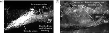
It is important to note that for the RJ supercavity in our experiment, the twin-vortex tubes still exist in addition to the re-entrant jet at the closure region, as shown in the side view of the supercavity structure in figure 12(a) and bottom view in figure 12(b). In the side view (figure 12
a), such twin-vortex tubes appear as a single rotating bubble column coming out from the closure region, carrying a large amount of gas from the supercavity. The gas flow rate in the twin-vortex tubes is denoted as
 $Q_{TV}$
. In addition, the foams of the toroidal vortex (associated with re-entrant jet) emerging from the liquid–gas interface carry additional gas (denoted as
 $Q_{RJ}$
). These foams further break into bubbles surrounding the twin-vortex tubes, and move downstream along with the gas flow inside the tubes. From the bottom view shown in figure 12(b), some bubbles from the toroidal vortex blend into twin-vortex tubes, with some gas emerging from the tube and breaking into bubbles.
Side view (a) and bottom view (b) of the closure region of the RJ supercavity under our experimental conditions. Both the toroidal vortex associated with the re-entrant jet and the twin-vortex tubes are observed.

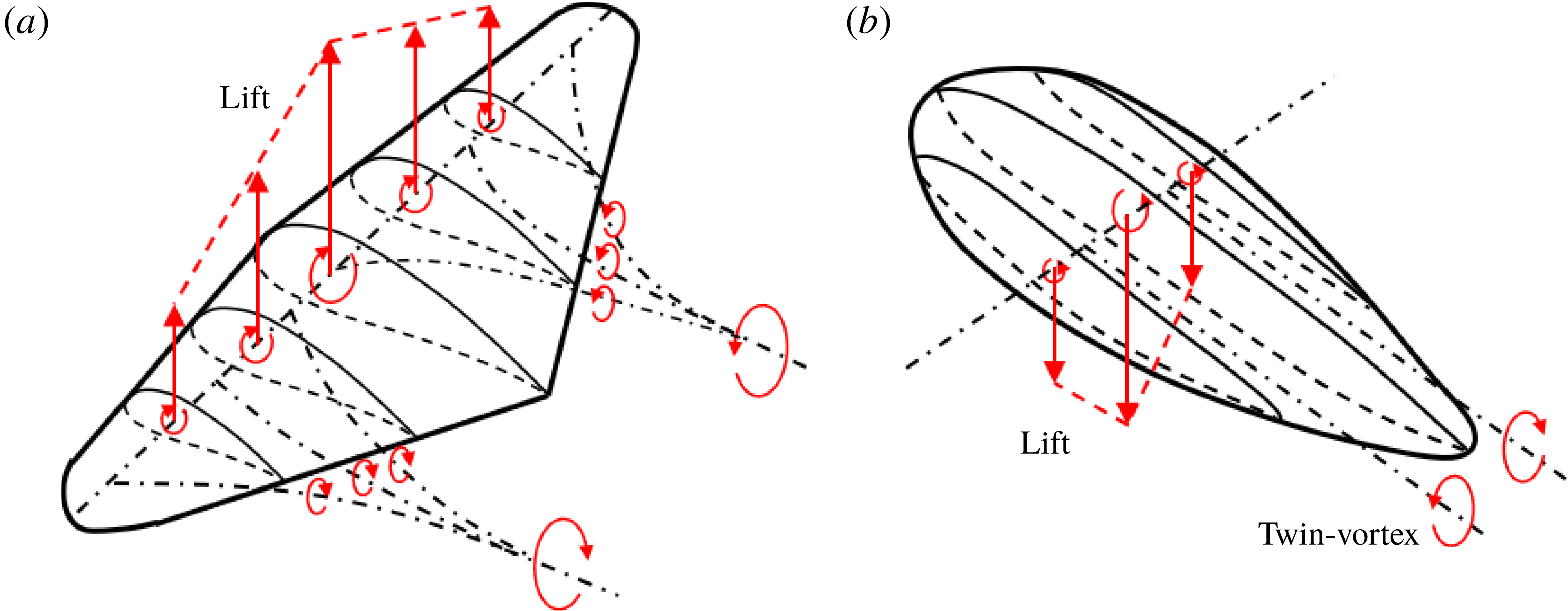
Since no prior studies on RJ supercavity have mentioned the presence of twin-vortex tubes in the RJ closure, here we provide a mechanism to explain this observation, as illustrated in figure 13. Generally, we think that the mechanism responsible for the formation of the twin-vortex tubes from a supercavity is analogous to the shedding vortices of an aircraft wing. Specifically, as shown in figure 13(a), due to the asymmetric shape of the airfoil of an aircraft wing, the flow distribution at the top surface deviates from that of the bottom surface. Such a deviation results in a net circulation, which induces a lift. According to the fundamentals of aerodynamics (for example, Simons & Simons Reference Simons and Simons1999), due to variations in the cross-section profile along the spanwise direction, the vortex formed by the flow circulation loses its strength along the whole wingspan. Due to Helmholtz’s first theorem, a vortex filament has constant strength along its length. Therefore, the aircraft wing sheds a street of streamwise rotating vortices from the trailing edge. Furthermore, the summation of the strength of the spanwise and streamwise vortices is conservative at all spanwise locations. This phenomenon has been thoroughly explained by the well-known Lanchester–Prandtl lifting line theory. Moreover, the shed streamwise rotating vortex street tends to merge into a pair of counter-rotating vortices while rolling up.
Schematic showing the formation of streamwise vortices due to the difference of velocity circulation along the spanwise direction for (a) an aircraft wing and (b) a supercavity.

Comparatively, as illustrated in figure 13(b), due to the buoyancy of gas bubbles, the profile of a supercavity results in a flow circulation which induces a downward ‘lift’ (Cox & Clayden Reference Cox and Clayden1955). For a supercavity, the flow circulation associated with the spanwise cross-section is maximum (bound circulation) at the meridian plane, and gradually decreases away from the meridian plane. This trend is similar to that of the aircraft wing shown in figure 13(a), except for the reversed direction. Accordingly, for the supercavity, the streamwise rotating vortex street merges into a pair of counter-rotating vortices at closure, but the rotating direction is reversed for each vortex. In addition, the pair of vortices causes the liquid–gas interface to deform and separate into twin-vortex tubes at closure, known as the TV closure.
In short, the TV closure originates from the 3D asymmetric shape of the supercavity. For the RJ supercavity in our experiment, the 3D asymmetry of the cavity is evident, and thus the twin-vortex tubes are clearly appreciable. The case is different from a number of prior studies on RJ supercavities (for example, Cox & Clayden Reference Cox and Clayden1955; Semenenko Reference Semenenko2001; Spurk Reference Spurk2002), where the coexistence of the RJ and TV closure was not clearly stated. In these prior studies, RJ supercavities were typically investigated under very high
 $Fr$
. Under such conditions, the gravity effect is negligible and the supercavity has an axisymmetric shape. Therefore, the flow circulation is zero at all spanwise locations and no vortex is shed downstream, resulting in the absence of the twin-vortex tubes. For the same reason, the TV closure does not appear for 2D supercavities which have a uniform cross-section shape along the spanwise direction (for example, the supercavity generated from a cylindrical cavitator).
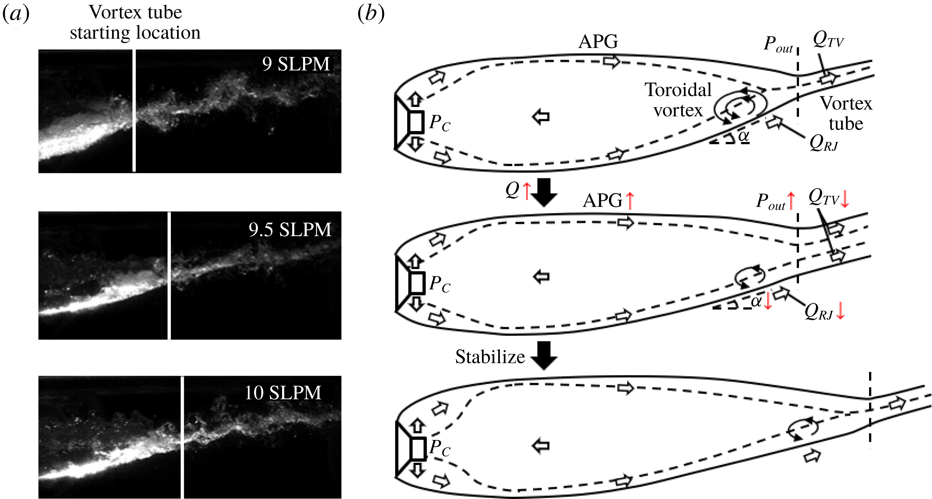
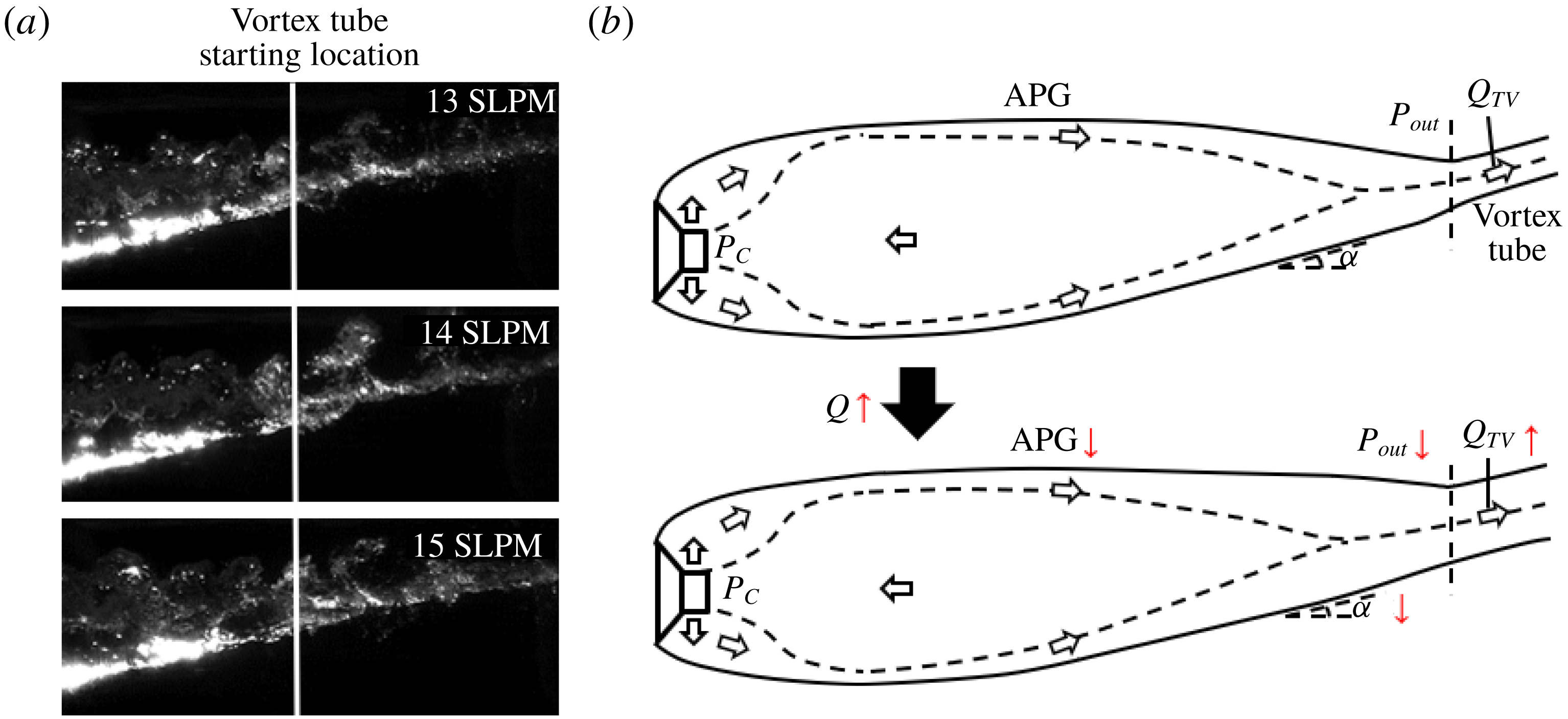
(a) Schematic showing the change of the internal flow, the geometry and the closure region of a RJ supercavity with increasing ventilation. (b) Images showing the change of the closure region of a RJ supercavity with increasing ventilation.

For RJ supercavity in our experiments, it is observed that the supercavity length grows and the toroidal vortex size reduces with increasing ventilation, as shown in figure 14(a). Such a trend can be explained based on our insights gained from the internal flow results in § 3.2 and the discussion of RJ closure generation at the beginning of this section. As mentioned earlier (figure 12) and shown in the upper schematic of figure 14(b), the gas leakage for a RJ supercavity is contributed by two mechanisms. One is from the shedding of the toroidal vortex associated with the re-entrant jet (i.e.
 $Q_{RJ}$
), and the other from the internal boundary layers that entrain gas and merge near the closure to form twin-vortex tubes (
 $Q_{TV}$
). For a stable RJ supercavity, the ventilation input (
 $Q_{As}$
) should be equal to sum of
 $Q_{RJ}$
and
 $Q_{TV}$
according to mass conservation. As the ventilation input increases under fixed
 $Fr$
, the supercavity changes its geometry, as illustrated in the middle and lower schematics of figure 14(b). In particular, the middle schematic shows a transient state during supercavity growth upon increasing ventilation. As it shows, an increased ventilation input (
 $Q_{As}$
) first causes the vortex tube at the closure to widen its diameter to ensure larger gas leakage, with a corresponding reduction of the incline angle of the bottom interface (
 $\unicode[STIX]{x1D6FC}$
). Such a reduction leads to a weaker external flow separation and a corresponding reduction in the gas leakage from the foamy toroidal vortices (i.e.
 $Q_{RJ}$
decreases). Meanwhile, due to weakening of flow separation, the pressure at closure (i.e.
 $P_{out}$
) recovers, as proved in past studies on hydrofoils (for example, Kubota, Kato & Yamaguchi Reference Kubota, Kato and Yamaguchi1992). Moreover, from our previous experiments (Karn et al.
Reference Karn, Arndt and Hong2016a
; Karn, Arndt & Hong Reference Karn, Arndt and Hong2016c
), the pressure at the backside of the cavitator (
 $P_{C}$
) stays approximately the same once the supercavity is formed, regardless of the ventilation input. Consequently, if the cavity length remains unchanged, the adverse pressure gradient within the supercavity increases, stripping a greater amount of gas out of the internal boundary layer as it moves downstream. This phenomenon is observed in the study of adverse pressure gradient boundary layers by Andersen, Kays & Moffat (Reference Andersen, Kays and Moffat1972). Correspondingly, the amount of gas entrained by the internal boundary layer at closure and leaking from the tubes decreases (i.e.
 $Q_{TV}$
decreases). Since both
 $Q_{RJ}$
and
 $Q_{TV}$
decrease upon an increase of (
 $Q_{As}$
) according to our assumption (i.e. supercavity length does not grow), under this condition, mass conservation is not satisfied (i.e.
 $Q_{As}>Q_{RJ}+Q_{TV}$
). As a result, more air is stored in the supercavity and the cavity has to elongate itself. After elongation, the cavity is able to entrain more air at closure (i.e. larger
 $Q_{TV}$
) to balance the ventilation input. The supercavity stops elongating when the internal boundary layer grows thick enough to fulfil the widened vortex tube at closure, as shown in lower schematic of figure 14(b). In contrast, reduction of
 $Q_{As}$
causes the RJ supercavity to shorten its length and increase the incline angle
 $\unicode[STIX]{x1D6FC}$
. It is worth noting that for
 $Q_{As}<9$
SLPM in our experiments, the external flow separation becomes so strong that
 $Q_{RJ}$
exceeds
 $Q_{As}$
. Mass conservation cannot be satisfied, and the supercavity keeps shortening and eventually collapses. Furthermore, it is also worth explaining why
 $Q_{As}=10$
SLPM is selected as the ventilation conditions of RJ supercavity used for visualization and PIV measurements in our experiments, but not lower ventilation input. Admittedly, with lower
 $Q_{As}$
, the toroidal vortex becomes larger (as shown in figure 14
a), and more appreciable differences may be observed between the RJ and TV supercavities. However, larger toroidal vortex rolls more water into the cavity. Driven by the vortex momentum and the adverse pressure gradient, more water droplets are observed intermittently impinging the liquid–gas interface. Therefore, the internal flow field is contaminated and cannot be used for PIV processing under these settings. Specifically, close to 50 % of the PIV images are disturbed with
 $Q_{As}=9$
SLPM. These droplet impingements are detrimental for achieving high-quality PIV measurements of the internal flows. Therefore, we limited our experiments to a minimum ventilation rate of 10 SLPM.
(a) Schematic showing the change of the internal flow, the geometry and the closure region of a TV supercavity with increasing ventilation. (b) Images showing the change of the closure region of a TV supercavity with increasing ventilation.

In our experiments, with a further increase of ventilation input, the supercavity closure transitions to TV closure. In contrast to the RJ supercavity, as shown in figure 15(a), we observe that the cavity length does not grow appreciably with increasing ventilation for the TV supercavity. This observation is supported experimentally and numerically by our previous studies (i.e. Cao et al.
Reference Cao, Karn, Arndt, Wang and Hong2017; Shao et al.
Reference Shao, Karn, Ahn, Arndt and Hong2017), which show the total length increase of a ventilated supercavity to be less than 10 % with doubling of the ventilation input. Compared to the RJ supercavity shown in figure 14(a), the TV supercavity has a longer streamwise extent, a wider vortex tube and a smaller incline angle (
 $\unicode[STIX]{x1D6FC}$
) for the bottom surface near the closure, as shown in the upper schematic of figure 15(b). Additionally, at the closure, the toroidal vortex vanishes and only the twin-vortex tubes remain, indicating all the gas leakage is contributed by internal boundary layer entrainment (i.e.
 $Q_{As}=Q_{TV}$
). Accordingly, the external boundary layer does not separate, so the water flow can be well approximated using potential flow theory, as established from many prior works on supercavitation (for example, Cox & Clayden Reference Cox and Clayden1955; Logvinovich Reference Logvinovich1972; Savchenko & Savchenko Reference Savchenko and Savchenko2012, etc.). As the ventilation input (
 $Q_{As}$
) increases, similar to that in the RJ case, the tube becomes wider to allow more air to leak from the tube, and the incline angle of the bottom surface (
 $\unicode[STIX]{x1D6FC}$
) decreases. However, with a decreased
 $\unicode[STIX]{x1D6FC}$
, the external water flow near the bottom gas–water interface experiences a weaker expansion as it moves towards the closure. According to potential flow analysis for flow over surfaces with varying curvatures (for example, Jackson & Hunt Reference Jackson and Hunt1975; Rhie & Chow Reference Rhie and Chow1983), the pressure at closure (i.e.
 $P_{out}$
) decreases with increasing local water flow velocities. Consequently, the adverse pressure gradient weakens and the internal boundary layer entrains more air at closure (i.e.
 $Q_{TV}$
increase), which is sufficient to fill the widened tubes. As a result, mass conservation is satisfied for the ventilation input and gas leaking (i.e.
 $Q_{As}=Q_{TV}$
), and thus the supercavity length does not increase appreciably.
4 Conclusions and discussions
In this paper, we present an experimental investigation of the internal flow of ventilated supercavities with two typical closure modes: RJ and TV. By introducing tracer particles through the ventilation line into the supercavity, we are able to perform flow visualization and the PIV measurements across the liquid–gas interface with in-house-developed image-distortion-correction code. The flow visualization reveals three distinct regions within the supercavity: the ventilation influence region near the cavitator, the extended internal boundary layer along the interface and the reverse flow occupying the large centre portion of the supercavity for both the RJ and TV supercavities. The PIV measurements enable us to quantitatively analyse the internal flow field inside the supercavity, including the streamwise and vertical extents of the ventilation influence region, streamwise growth of the internal boundary layer and the reverse flow. Compared to the RJ supercavity, the results indicate the TV supercavity yields a longer vertical extent of the ventilation influence region, a thinner internal boundary layer and a stronger reverse flow. Using the results of the internal velocity field, we show that the estimated gas flow rate carried in the reverse flow first increases as it moves upstream from the closure region, reaches a maximum around the location of the maximum cavity diameter, and then decreases as it approaches the cavitator. Successively, based on above-mentioned trends, a general picture that depicts the internal gas circulation for a ventilated supercavity is proposed. Specifically, upstream of the location of the maximum cavity diameter, the gas enters the forward flow from the reverse flow due to the strong entrainment associated with ventilation injection and the effect of cavitator blockage. Here the forward flow includes the internal boundary layer and the forward moving portion of the ventilation influence region. At locations further downstream, the gas is stripped from the internal boundary layer and enters the reverse flow due to the increasing adverse pressure gradient in the streamwise direction. The reverse gas flow eventually disappears at the closure region when the internal boundary layer developed from all circumferential locations at the 3D interface merges. Different from the assumption of Spurk (Reference Spurk2002), our results clearly demonstrate the occurrence of the reverse flow and gas exchange between the internal boundary layer and the reverse flow throughout the supercavity. Our work provides the first experimental evidence that is in general agreement with the simulation and analytical work from Kinzel et al. (Reference Kinzel, Lindau and Kunz2009). However, our work delivers significantly more detailed information on the growth trends of the reverse flow and the internal boundary layer that was not available in the literature.
Furthermore, by combining visualization results of supercavity geometry and closure patterns, we further explain the influence of the gas leakage mechanism on supercavity growth and the closure transition. Specifically, based on visualization of the change in cavity geometry during the RJ to TV supercavity transition, we attribute the formation of RJ closure in our case to flow separation at the water side. The separation is caused by the strong adverse pressure gradient associated with the high incline angle of the bottom liquid–gas interface. In addition, in contrast to a number of prior studies on RJ supercavities (for example, Cox & Clayden Reference Cox and Clayden1955; Semenenko Reference Semenenko2001; Spurk Reference Spurk2002), the coexistence of the toroidal vortex associated with the re-entrant jet and the twin-vortex tubes is observed in the RJ supercavity in our experiments. In particular, the presence of twin-vortex tubes in our RJ supercavity is shown to be inherently due to the 3D asymmetric shape of the ventilated supercavity formed under low
 $Fr$
. The coexistence of the toroidal vortex and twin-vortex tubes leads to two gas leakage mechanisms for the RJ supercavity, i.e. one associated with the shedding of toroidal vortices (
 $Q_{RJ}$
) and the other associated with the gas entrained by the internal boundary layer and leaking from the twin-vortex tubes (
 $Q_{TV}$
). Based on these two gas leakage mechanisms, a physical explanation on the supercavity growth trends and the closure transition (i.e. from RJ to TV) is provided. Specifically, for the RJ supercavity, with increasing ventilation input under the same
 $Fr$
, the incline angle of the bottom liquid–gas interface decreases. The decreased incline angle leads to reduced flow separation and a stronger adverse pressure gradient inside the supercavity, and consequently a decrease of
 $Q_{RJ}$
and
 $Q_{TV}$
if the cavity shape remains unchanged. Therefore, to balance the increasing ventilation input, the supercavity body is elongated to ensure more gas is entrained by the internal boundary layer at closure and leaks from the twin-vortex tubes. With further increase of the ventilation, the RJ closure disappears when the incline angle drops below the critical value for external flow separation, while the twin-vortex tubes remains at the closure, resulting in the transition from the RJ to the TV supercavity. In comparison, for the TV supercavity, increasing ventilation input also results in a decreased incline angle of the liquid–gas interface. However, since the flow separation does not present (i.e. no
 $Q_{RJ}$
), the pressure at the closure decreases with increasing ventilation, causing a decreased adverse pressure gradient and increased
 $Q_{TV}$
accordingly. As a result, the supercavity is able to balance the ventilation input with increasing
 $Q_{TV}$
, and the cavity length does not show appreciable variation.
Our present study provides experimental support to the unified framework for explaining the closure mode variation proposed in Karn et al. (Reference Karn, Arndt and Hong2016a ). Specifically, based on the internal velocity field, our present studies show evidence of a substantial non-uniform pressure distribution in a ventilated supercavity and the stronger adverse pressure gradient for the TV supercavity, consistent with the hypothesis from Karn et al. (Reference Karn, Arndt and Hong2016a ). However, due to the measurement limitations discussed later in this section, our study is not able to offer a comprehensive assessment of the framework in Karn et al. (Reference Karn, Arndt and Hong2016a ), which requires internal flow measurements for many other closure modes and flow conditions beyond the two cases presented here. Moreover, in comparison to the work in Karn et al. (Reference Karn, Arndt and Hong2016a ), our study adds new physical insights into the transition from RJ to TV closures and reveals additional features of RJ closures. Particularly, we observe the presence of twin-vortex tubes in the RJ closures classified in Karn et al. (Reference Karn, Arndt and Hong2016a ). This information was missing in Karn et al. (Reference Karn, Arndt and Hong2016a ) since it only employed side-view images for closure mode classification, while the twin-vortex feature is substantially more evident from the bottom-view images. Besides, the twin-vortex tubes in the RJ closures are stabilized once the RJ supercavity is formed. Therefore, this closure is different from the TVRJ closure studied in Karn et al. (Reference Karn, Arndt and Hong2016a ), which refers to as an unstable closure mode shifting between the RJ closure and the TV closure.
Finally, we would like to point out a number of limitations of our current measurements; the corresponding caution needs to be taken about our results as well as the suggestions for future investigation.
First, the particle seeding approach employed in our current experiments constrains us from extending our internal flow measurements to other closure modes and flow conditions. Specifically, in the current study, the particles are seeded through the same ventilation line as the gas, which makes it difficult to control the seeding concentration and the ventilation rate independently. This constraint limits our measurements to relatively low
 $Fr$
and low
 $C_{Qs}$
, covering only the bottom left corner of the closure maps presented in Karn et al. (Reference Karn, Arndt and Hong2016a
). Such a limitation can be addressed by introducing a separate particle seeding line into the cavitator or generating seeding particles locally inside a ventilated supercavity. Both approaches require significant modification of the current cavitator. For the approach using a separate seeding line, we need to consider with caution the effect of the additional ventilation used for transporting seeding particles into the supercavity on the internal flow field.
Second, the hydrofoil employed for mounting the backward-facing cavitator produces a non-negligible wake that adversely influences internal flow measurements. The wake induces appreciable disturbance on the upper interface of the supercavity interface, which grows and eventually affects the bottom interface at downstream locations. Such a disturbed interface leads to image distortion and noise, limiting our PIV measurement region (i.e. where valid velocity vectors can be extracted from image cross-correlation) to the bottom half and approximately the upstream one-third portion of the entire supercavity. Therefore, we are unable to obtain the internal flow field near the closure region, including the region where the internal boundary layer is expected to merge and the reverse flow disappears. In addition, the hydrofoil wake can impose a slight modification of the geometry of the supercavity upper surface. Correspondingly, the internal boundary layer developed along the upper liquid–gas interface (not available from our measurements) may yield some differences in gas entrainment compared with the one measured at the lower interface. Such upper surface modification can also cause some uncertainties in the measurement of the 3D supercavity geometry, and thus the results of our image distortion correction. Considering this constraint associated with the usage of a backward-facing cavitator, we plan to shift our attention to the ventilated supercavity generated from a forward-facing cavitator for future experiments. With a forward-facing cavitator, where the mounting structure sits inside the supercavity, the supercavity interface is significantly less disturbed than that of the current case, allowing the study of the internal flow structures over a broad range of flow conditions, including the unsteady cases presented in Shao et al. (Reference Shao, Wu, Haynes, Arndt and Hong2018).
Third, due to limited spatial resolution of the present PIV measurements, the velocity profile of the internal boundary layer cannot be resolved at locations very close to the liquid–gas interface. The lack of such information limits our ability to directly estimate the ventilation gas carried within the internal boundary layer. The spatial resolution of our PIV can be further increased with the improvements to the camera sensor, imaging optics and light-sheet generation optics. However, such improvements of the hardware would still be unable to provide sufficient resolution to fully resolve the boundary layer. Other advanced near-wall 3D flow imaging approaches, such as digital inline holography (for example, Toloui, Mallery & Hong Reference Toloui, Mallery and Hong2017; Kumar & Hong Reference Kumar and Hong2018), may offer potential solutions for such measurements.
Fourth, our current measurements cannot be used to derive the pressure field inside the supercavity. Therefore, it is difficult for us to directly quantify the non-uniform pressure distribution and adverse pressure gradient inside a ventilated supercavity using the current velocity field data. Such internal pressure field measurements can be potentially achieved if high-fidelity acceleration field can be extracted from time-resolved planar PIV measurement and if the supercavity can be approximated as an axisymmetric body (Liu & Katz Reference Liu and Katz2013). For the ventilated supercavity generated from the forward-facing cavitator as mentioned earlier (Shao et al. Reference Shao, Wu, Haynes, Arndt and Hong2018), the pressure distribution along the streamwise direction within the supercavity can be readily obtained using a series of pressure taps installed on the horizontal supporting strut.
Finally, as suggested from the present work, it is the interplay between the internal gas flow and external water flow that determines the gas leakage and closure transition. However, only the internal flow-field measurement is obtained in the current study. Ideally, the simultaneous measurements of internal and external flow fields are needed to elucidate some of the observed trends. Particularly, PIV measurements of the flow field on the water side need to be performed at the external flow separation region near the closure, which is not available due to the influence of strong laser reflections in the current study. Future experiments will consider using the combination of fluorescent particle seeding in the water and a band-pass filter installed on the camera to block the laser reflection and extract the particle signals.
Acknowledgements
This work is supported by the Office of Naval Research (Program Manager, Dr T. Fu) under grant no. N000141612755. We thank E. Steen, C. Ellis and J. Tucker for their mechanical support and advice during the water tunnel experiments.
Supplementary movies
Supplementary movies are available at https://doi.org/10.1017/jfm.2018.1006.