

The variation in cabinet stability in multiparty political systems is notorious. Some cabinets have survived their entire electoral cycle even under minority governments, while others have displayed persistent instability even when the coalitions on which they were based exceeded the minimum majority by a wide margin. This may well explain the voluminous scholarly literature on the factors affecting cabinet duration. Political polarization is often invoked as a possible explanation for political stability, but – as we show in the following sections – the arguments linking polarization to political stability are varied and often inconsistent. The same applies to the empirical relationships between measures of political polarization and cabinet stability. This suggests a need for a new perspective on the relationship between political polarization and stability.
This study offers a new strategy to tackle this relationship. Using bargaining theory, we argue that the level of polarization in political systems is a powerful indicator of the opportunities that parties have to renegotiate coalitions. As political polarization – the existence of ideologically cohesive and distinct party blocks, controlling roughly equal seat shares – increases, parties have fewer opportunities to form coalitions without resorting to elections. This induces considerable constraints on the initiation and management of political crises.Footnote 1 Such crises are likely to be resolved without reshuffling the party basis of the cabinet. Consequently, political polarization tends to prolong cabinet duration.
We offer a new approach to the conceptualization and measurement of political polarization that draws on Social Networks Analysis (SNA). SNA is a methodology for the analysis of structures of relationships, and as such is eminently suitable for the study of political processes. However, until recently this approach has been under-utilized in the study of comparative political systems. Our measure of political polarization combines information about party ideology, inter-party distances and party size. It measures the structure of political systems in terms of possible and actual coalitions. With this measure we identify proto-coalitions ex ante and explain how the bargaining environment affects cabinet survival, an aspect which is absent from most other measures of polarization.
The study is structured as follows. In the next section, we summarize the literature and state our theory about the effects of political system polarization on cabinet stability. The third section critically reviews the existing measurements of polarization, and discusses the network analytic measure of political polarization. The next section outlines the research design and then we discuss the empirical results. We conclude by discussing the theoretical and empirical implications of our results.
Theory
Political parties are rational utility-maximizers seeking to affect policy in accordance with their political preferences. Which coalition they decide to join depends on two key variables: (a) the similarity between the projected coalition’s policies and the party’s ideal point, and (b) the probability that the party would affect the coalition’s policy. The similarity between the party’s ideal point and the coalition’s policies is a function of the distance between the party’s ideal point and the coalition’s ideal point. However, the effect of a given party on a coalition’s policy depends on the cohesion of the coalition; the more cohesive the coalition, the less likely its policy is to deviate from its own ideal point. Parties are likely to defect from a given coalition to the extent that (a) the coalition’s policies are less similar to the party’s preferred policies, and (b) there exist other coalitions that offer a party a higher expected utility.
The implication for coalition stability is straightforward. A coalition is more stable the less likely its members are to defect. Coalitions that comprise parties that are either satisfied with the coalition’s policy or have no better alternatives are more likely to survive political crises than coalitions that are unstable in this sense. This leads directly to our conception of political polarization. Political systems that exhibit high levels of polarization reflect a set of relatively cohesive, discrete and minimum winning coalitions. Political parties in highly polarized systems have few feasible alternatives to the coalition they are currently in. Moreover, the coalition’s policy – due to its cohesiveness – generally approximates their ideal points.
In contrast, as political polarization declines, any one of the following characteristics of coalition structures changes: the proto-coalitionsFootnote 2 tend to be politically diverse in terms of members’ ideal points; there is considerable overlap in party membership among proto-coalitions; or the proto-coalitions – defined endogenously in terms of parties’ positions – tend to be excessively large. This suggests that parties in any ruling coalition may opt out to the extent that an alternative coalition exists that offers them a greater potential benefit.
This conception is in line with other studies. Lupia and Strøm emphasize the importance of the bargaining environment. They argue that rational responses of political actors to the bargaining environment define the timing of cabinets’ terminations. Nyblade suggests that it is the relative distance between parties, rather than the absolute distance, that matters for cabinet survival. He finds that a measure of relative government diversity (the difference between the government’s left–right policy and that of the most compact majority coalition that excludes the largest coalition party) has a significant negative impact on cabinet duration. Warwick finds that ‘party horizons’, namely ‘the maximum extent of policy compromise that they are prepared to undertake in order to participate in government’ matter for both cabinet formation and duration.Footnote 3
While our approach bears some similarity to Warwick’s policy horizons argument, it is based on the ex ante possible coalition structure, not on ex post coalitions (see the discussion below on the importance of polarization measurement based on ex ante attributes). By identifying the proto-coalitions, we can model the bargaining environment within each electoral cycle and determine the likelihood of cabinet survival based on political polarization. Accordingly, we can also frame the intuition of the model in terms of parties’ strategies and attempts to predict which of the proto-coalitions would actually form, which parties are likely to defect from the coalition under certain circumstances, and so forth.
An important issue arises when we consider the relationship between which coalitions form and how long they last. If political polarization were based only on the size of the parties and a fixed set of parties within an electoral cycle, then if our theory held, no coalition – once formed – would end prematurely. Regardless of the level of polarization, parties would form optimal coalitions, and these coalitions would have to survive political crises because members would find all other coalitions inferior to the current one. However, this is neither the implication of our theory, nor is it the observed reality. Since polarization is based on ideological positions as well as on size, the nature of proto-coalitions, and thus the political polarization of the system can change as parties shift their positions within electoral cycles. When that happens, everything changes and parties reassess their bargaining opportunities. Thus, a coalition that was optimal at one point in time need not be optimal at another. Moreover, our conception of political polarization suggests that it should affect cabinet duration even if all parties maintained their ideological positions throughout the electoral cycle. This is so because in many cases there is no single best coalition. As polarization declines, more proto-coalitions are ‘optimal’ in the sense that they form part of the bargaining core and are thus part of a multi-equilibrium environment. In such cases, the ability to shift from one coalition to the other is not as costly as it is when the system is highly polarized. So, which coalitions form and how long they last may be related. But this relationship is only part of the more general story that our concept of political polarization tells us about the bargaining environment of parties.
Most conceptions of polarization – including our own – view it as an emergent property of the system. This means that polarization is a function of the characteristics of the individual elements of the system – political parties – and the relationships that exist between them (i.e., their ideological similarity or differences). Thus, the elements of this concept, as well as its overall systemic character, are believed to affect the calculations and behaviour of individual parties (for example, define what kind of coalitions would form), as well as the systemic outcomes of these calculations (such as political stability). At this point, however, we focus on the systemic impact of political polarization. Accordingly, the following hypotheses serve as the centre of our investigation.
HYPOTHESIS 1. Ceteris paribus, the higher the level of political polarization in a political system, the longer the duration of cabinets that rely on political coalitions.
HYPOTHESIS 2. Ceteris paribus, the higher the level of political polarization in a political system, the fewer the number of cabinets existing within a given electoral cycle.Footnote 4
Conceptualizing and measuring political polarization
Cabinet duration is typically taken as a synonym for political stability in parliamentary systems. Since the late nineteenth century, students of parliamentary democracy have explored theoretically and empirically factors that affect cabinet duration. In one of the most representative studies of attributes, Warwick found that cabinet majority status, minimal winning coalition status, ideological cleavages within the cabinet and the number of parties in the government can significantly affect the tenure of governments.Footnote 5
In more recent works, the focus of the analysis has shifted to understanding the underlying hazard rates and the strategic interactions between actors for cabinet duration.Footnote 6 The bargaining environment was also the focus in the work of Diermeier, Eraslan and Merlo, who have developed a bargaining model of government formation and duration using a structural equation model.Footnote 7 However, they have treated preferences over potential coalition partners as essentially random, i.e. not systematically related to exogenous policy preferences or ideological similarities/differences. In this study, we develop a measure of system polarization, which relies on the information about policy preferences and parliamentary sizes of political parties, and argue that this polarization index has a significant effect on cabinet termination in West European democracies. Our work not only contributes to this recent literature but also provides a new perspective focusing on the effect of the structure of the political system – defined in terms of polarization – on the strategic behaviour of political parties. A subsequent study of ours will extend the social networks approach by interacting political polarization with the strategic interaction among parties in cabinet formation and termination processes.
System polarization has often been considered an important determinant of cabinet duration. The modal measure of political polarization has been the proportion of seats held by extreme parties. Powell introduced this measure and found that as this proportion increases, cabinets were more likely to collapse.Footnote 8
Nevertheless, Warwick argued that polarization, measured in terms of extreme party seat shares, does not tell us much about the bargaining environment that parties face.Footnote 9 By using several different data sources (expert surveys, public opinion surveys and Comparative Manifesto Project data), Warwick positioned government parties by their relative parliamentary strength on four ideological dimensions: Left–Right, clerical–secular, regime support and materialist–postmaterialist. Next, he measured the total range of a government on each scale as well as the standard deviation of the distribution and presented his conclusion that the ideological diversity index has a negative effect on cabinet duration.
Gross and Sigelman developed an ideological polarization index measuring deviations within each system from an ‘ideological centre of gravity’.Footnote 10 Although this measurement of system polarization reflects polarization better than do seat shares of extreme parties, it still relies on the position of parties along a single left–right dimension. Moreover, it does not take into account possible alternative coalitions that can form in the system.
Esteban and Ray and Duclos et al. have offered an axiomatic approach to the measurement of polarization that overcomes various biases included in simple measures of income inequality, such as the Gini index.Footnote 11 Their polarization index is based on three key parameters: the cohesion of units (individuals, parties), their relative size, and the absolute distance between units. Rehm and Reilly use this index to compare political polarization in the United States to that in other political systems.Footnote 12 Despite the fact that this polarization index appears to be more thorough than the other indexes, it is based on a number of arbitrary assumptions (such as a small number of groups, or a uniform identification index). It was also shown by Maoz that this index manifests an extremely high correlation with the number of groups and the number of members in each clique.Footnote 13 This suggests – in our case – that polarization could be tapped simply by the number of political parties.Footnote 14
Despite the diversity of definitions mentioned above, most measures of polarization share several problems:
1. Existing measures are based either on the attributes of the units/groups or on their relationship and organization; few – if any – combine both.
2. Most existing measures presuppose a division of the system into discrete blocks. Membership of units in these blocks is pre-defined. For example, some of the studies reviewed above pre-determined polarization by the number, identity and/or attributes of the parties that compose the coalition, or by the assignment of labels to parties such as ‘extreme right’ or ‘extreme left’. Yet the division of the system into coalition and opposition is endogenous; it is derived from the calculations of, and relationships between, political parties. The polarization of a political system may be a function not only of its actual division into coalition and opposition, but also of other proto-coalition/opposition configurations that need to be determined endogenously.
3. Most measures of polarization assume discrete groups (such as coalition/opposition). In real life, however, political parties cannot be placed singularly in a given group. By arbitrarily assigning units to groupings, we miss complex possible relationships in the system. In our case, this implies that a given political party could – given some pre-defined criteria such as ideology, seat shares or a combination of both – qualify as a member in several proto-coalitions. Whether or not a party finds itself in a particular coalition is a function of an actual bargaining process. From a theoretical point of view, a measure of political polarization should be based on ex ante attributes and theoretically specified processes, not on ex post political developments.
4. The boundaries of polarization – what constitutes maximum and minimum polarization – are not always well defined. A desideratum of a measure of polarization that allows comparison of political systems across time and space is a well-defined continuum in terms of its end points. This implies that the characteristics of situations which define maximum and minimum polarization should have intuitive interpretations that are theoretically sound. In the context of party systems, the cases of maximum polarization and minimum polarization should have meanings corresponding to our intuitive understanding of what constitutes a maximally (or minimally) polarized system.
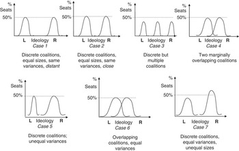
We demonstrate these problems in the conversion of abstract concepts of polarization to empirical measures by the distributions of political coalitions in Figure 1 below.
Problems of defining political polarization

Each case in this figure represents a set of proto-coalitions in a party system. A distribution is a set of party ideal points that defines the coalition. The variance of a given distribution reflects the ideological diversity of the parties making up this coalition. To simplify this presentation, we use a single dimension but this applies to a multidimensional ideological space without loss of generality. A coalition can be composed of 1, 2, …, k political parties. The seat share axis is the proportion of the parliamentary seats accounted for by the parties making up the coalition.
Consider Cases 1 and 2. In both cases, the two proto-coalitions are equal in size, and all of the political parties in the system are located in one of these coalitions. No party overlaps across the two proto-coalitions, and the ideological diversity of both coalitions is identical. Intuitively, both cases show a high degree of polarization. However, Case 1 suggests greater polarization than Case 2 because the ideological distance between the parties is larger in the former case than in the latter. A party shifting from one coalition to another would have to go through a larger ideological change in Case 1 than it would in Case 2. This comparison allows a fairly straightforward intuitive interpretation of degrees of polarization.
Consider, in contrast, the comparison between Case 3 and Case 4. Case 3 represents a configuration of three proto-coalitions, each of them discrete in terms of its party make-up, each of which is ideologically cohesive, but none of them constituting a majority. By contrast, in Case 4 each of the two coalitions controls a majority, but they are more diverse ideologically, and some of the parties are members of both proto-coalitions. Which case reflects more polarization?
To complicate matters, consider Cases 5–7. Case 5 reflects two discrete coalitions; each has 50 per cent of the seats, but one is more cohesive than the other. In Case 6, we have two equally large coalitions that have some common parties in both. Is Case 6 more polarized than Case 5 or vice versa? How about Case 7, in which we have two discrete coalitions but one of them controls a more than 50 per cent majority while the other does not?
This comparison clearly demonstrates that – with the exceptions of Cases 1 and 2 – it is difficult to choose between any other pair in these examples in terms of which represents a higher degree of polarization. There seem to be multiple factors that affect our intuitive notions of polarization. When we place greater emphasis on the ideological homogeneity or diversity of the coalitions and on the distance between them, some examples seem to offer a greater degree of polarization than others. When we emphasize the extent of party overlap across coalitions as a key determinant of polarization, we get a different ranking of the polarization-related political systems. Finally, if the size of the coalitions matters, then cases in which coalitions are roughly equal would reflect a higher polarization than cases in which coalitions vary in size.
Formally, we introduce the following notation. Define a system as a set of N = [1, 2, …, n] units (in our case, political parties). The units can be grouped together into a set of K cliques, where each clique k is a grouping of [1, 2, …, n] units according to a specific rule. Let S = [s 1, s 2, …, sk] be the set of units that belong to each of the cliques. The only restriction on the structure of cliques (we elaborate on this later on) is that no clique can be a proper subset of another clique (ki⊄kj ∀ k ∈ K). We define the cohesion of a given clique as

,where d is some characteristic of clique members (such as parties’ ideal points). Finally, define the size (power) of a clique as a set P = [p 1, p 2, …, pk].Footnote 15 The boundaries of political polarization as we intuitively think about this concept are defined in the following manner. Maximum polarization refers to what international relations theorists refer to as strict bipolarity. This is reflected by a system that has all of the following characteristics:
1. The system is divided into two cliques (K = 2).
2. The cliques are discrete; there is no overlap of units across cliques (k1 ∩ k2 = ∅).
3. The cliques are equal in size (power) (p1 = p2).
4. The cliques are cohesive in terms of the relationships among units that form them (c1≅c2 → 1).
Thus, maximum political polarization in a party system is obtained when there are exactly two proto-coalitions; these coalitions are discrete – no party overlaps across them; each accounts for exactly 50 per cent of the seats; and both are highly cohesive (the variance of the ideal points of the parties in each is rather small). Since all four conditions need to be fulfilled to characterize a system as maximally polarized, it is evident that the trade-offs between any two conditions reduce polarization. Minimum polarization (polarization = 0) is obtained when the rule that assigns units to cliques produces a single clique. Once this happens, the other elements of the polarization equation follow.
All of these factors play a central role in the bargaining game that defines the effect of polarization on cabinet stability. Our focus in the present study is on developing a general measure of polarization and estimating the effect of polarization on cabinet duration. Hence, we do not specify here the formal model of cabinet stability. Rather, we discuss the intuition of the model and explain how political polarization in the sense discussed above is expected to affect cabinet duration.
Social Network Analysis and the Network Polarization Index
For those not familiar with Social Networks Analysis (SNA), a brief (and admittedly superficial) review of the approach and its key concepts is in order. A social network is a set of units (nodes) and a rule that defines whether, how and to what extent any two units are tied to each other. In our case, a network is a set of parties in a given country during a given electoral cycle. The rule that defines the ties between parties is the ideological distance between the parties.
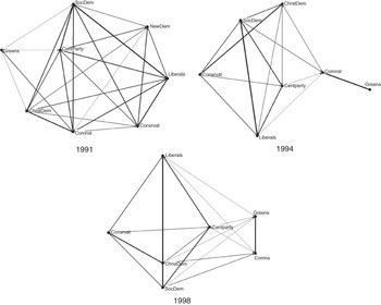
SNA is a general framework that allows systematic measurement and analysis of structures of relationships in and across networks. It is widely used in sociology, social psychology and organizational behaviour.Footnote 16 Social networks can be represented and analysed via graph theory or via matrix algebra. In order to illustrate the representation of a party system as a set of social networks, consider three electoral cycles in Sweden. This is done in Figure 2.
Party networks in Sweden – three electoral cycles, 1991–98

Each party in Figure 2 is represented by a circle and next to it the party’s abbreviation. Lines represent ties between parties and the width of the lines reflects the extent to which the parties’ positions – as expressed in their manifestos – overlap. Wider lines reflect a greater degree of overlap. If two parties have a zero or negative overlap in terms of their issue positions (meaning that the positions of these parties are diametrically opposed on at least some issues),Footnote 17 then these parties are not connected. In 1991, there were eight parties, with the Centre party, the Social Democrats, the Liberals and the Christian Democrats having the strongest ties to all other parties, and the Green party being relatively isolated (negative ties to the Conservatives, the New Democrats and the Liberals).
This isolation of the Green party was accentuated in 1994 with ties only to the Communists. The Social Democrats seem to have had, on average, more and stronger connections to all other parties except the Greens. Note that in 1994 there were only seven parties in the Riksdag (the Swedish Parliament), the New Democratic party having disappeared. In 1998, the general pattern of relations was similar to that of the previous two electoral cycles with one notable exception: the Green party came out of its relative ideological isolation and maintained positive – if weak – ties to other political parties.
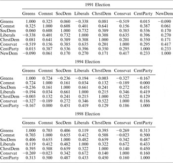
This graphic presentation helps illuminate the structure of political ties between parties based on their manifestos. An alternative presentation of such networks is via matrices. Generally speaking, SNA deals with two types of networks: relational and affiliational. A relational network is a socio-matrix S of order n × n where entries sij reflect the existence, nature and magnitude of a tie between units i and j. A relational network can be symmetrical (sij=sji ∀ i,j∈N) or asymmetrical (sij ≠ sji). In our example, all relational networks are symmetrical. An affiliational network (also called a two-mode network) is represented by an affiliation matrix A of order n × m where rows represent the n units and columns reflect events, institutions or concepts. Each entry aik reflects the existence, nature or magnitude of affiliation of unit i with event, institution or concept k. We demonstrate these two types of networks below.
Assume a system of N parties that defines their policy positions on m issues. This defines an affiliation network on an n × m matrix A with rows representing parties and columns representing issues. Each entry in this matrix aim reflects the position of party i on issue m. This position can be defined either as an ideal point on dimension j, or – as in our data, a proportion of the party’s manifesto devoted to a certain issue position (such as for or against immigration, for or against integration in the European Union, and so forth). Depending on the definition of parties’ positions (as ideal point or proportion of their manifesto’s focus on an issue), there exist a number of alternative methods to convert matrix A into a socio-matrix S that reflects the strength of ideological ties between parties. Here, we use the conventional SNA approach where S = A× A′. Each entry in the socio-matrix sij reflects the extent and type of overlap between the positions of parties i and j across the m issues. Off-diagonal entries sij can vary from −1 (that reflects a diametrically opposed set of positions of the parties across the issues, but also that the two parties had a perfectly matched emphasis on the same issues, i.e. the proportion of election manifestos dedicated to the issues of interest are the same across parties) to +1 (reflecting a perfect match and a perfect positional alignment of parties across the m issues). Diagonal entries sii reflect the diversity of issue coverage in the manifesto of party i: these vary between 0 (for single-issue parties – that is, parties whose manifesto addressed only one issue) and 1 (when a party had devoted an equal amount of space in its manifesto over 2, 3, or …, m issues).
To illustrate this representation, consider Table 1, which shows the three electoral cycles in Sweden (illustrated in Figure 2) as three socio-matrices. In order to enable meaningful cross-party comparison, the original socio-matrices are diagonally standardized. That is, each entry in the original socio-matrix is divided by its smallest corresponding diagonal entry. The entries in the modified socio-matrix Ś are defined as śij=sij/min (sii, sjj), where sii and sjj reflect the diagonal entries corresponding to the row or column index. This implies that the overlap in the positions of parties i and j is expressed as a proportion of the less ideologically diverse of these two parties. The reason for this standardization is fairly straightforward. The extent to which the ideological positions of any two parties can overlap is a function of the ideological diversity of both. Two multi-issue parties have a greater chance for ideological overlap and difference compared to two parties, one of which addresses multiple issues, and the other being a single-issue party.
Socio-Matrices of Swedish Party System, 1991–98

The Network Polarization Index (NPI) developed by Maoz has two essential components: clique polarization and clique overlap.Footnote 18 A clique is a closed subset of the network, that is, a subset of units that have direct ties to each other (at or above a certain level). A clique cannot be a proper subset of another clique. Thus, any two cliques [k, r ∈ C] must differ with respect to at least two members (at least one member of k is not a member of r, and at least one member of r is not a member of k).
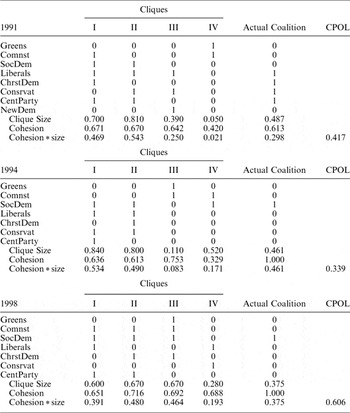
We start the discussion of the NPI by defining the clique polarization index, CPOL. In our context, cliques reflect possible coalitional configurations. A proto-coalition is a set of parties that has ideological connections to each other above a certain threshold. In our context, such a threshold is defined as the average ideological overlap in the standardized socio-matrix, Ś.Footnote 19 The clique derivation algorithm of SNA allows enumeration of all proto-coalitions that meet this criterion. These coalitions are exemplified by the Clique Affiliation (CA) matrices shown in Table 2 for the three Swedish electoral cycles.
Clique Affiliation Matrix (Proto-Coalitions) in Sweden, 1991–98

The question of which coalitions could be formed, in contrast to those that are actually formed, and of the duration of the actual coalitions is an interesting and central one. We leave it, however, to a future study. Here, we use the examples in Table 2 to highlight the CPOL index. Briefly, CPOL is defined as:
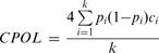
,where pi and ci are, respectively, the seat share and cohesion of coalition i (as defined in the first equation above), and k indexes all proto-coalitions. Intuitively, clique polarization measures the extent to which each coalition is polarized with respect to other members of the party system who are not part of the coalition. This is standardized by the maximum possible polarization that can occur in a system of k coalitions. CPOL varies between 0 when k (and thus pi) =1 (that is, there exists only one coalition that encompasses all parties – the grand coalition), and 1 when k = 2, p1 = p2 = 0.5, ci = cj = 1 (that is, there exist two perfectly cohesive coalitions, each of which controls half of the seats in the parliament – perfect bipolarity).
In reality, however, CPOL is seldom at one of its end points. This implies that at least some of the proto-coalitions overlap in terms of party membership. This is evident in Table 2. The actual polarization of the political system, therefore also depends on the extent to which individual members overlap across cliques. This leads us to the Clique Overlap Index (COI). To obtain this index, we utilize the clique overlap matrix (CO). We obtain CO by CO= CA′× CA. The CO matrix is a k × k matrix that has the following structure: diagonal entries coii reflect the number of units in each clique (in our case, the number of parties in each of the proto-coalitions), off-diagonal entries coij reflect the number of units that overlap across cliques i and j (in our case, the number of parties that two coalitions share in common). We standardize the CO matrix such that the standardized matrix  has entries defined as:
 where coijj is the column diagonal. Using this matrix, we calculate COI as:

.
COI varies between 0, when none of the cliques overlaps with another in terms of units (that is, when all proto-coalitions are discrete), and approaches 1, when there is maximum overlap between cliques.Footnote 20
Taking both CPOL and COI, we can generate the Network Polarization Index (NPI) as: NPI = CPOL × (1−COI). Clearly, NPI = 0 when CPOL = 0 (and by definition in such a case, COI = 0 because this implies that all nodes are in a single clique – the grand coalition). Likewise, NPI = 1 if both CPOL = 1 and COI = 0. These two conditions can be met only if two discrete, equally powerful and highly cohesive coalitions exist – that is, if the system is strictly bipolar.Footnote 21
Maoz discusses the general properties of the NPI and compares this index to other polarization indices (for example, Duclos et al.) via Monte Carlo simulations and real data.Footnote 22 Here, however, it is important to emphasize the kind of information that this index utilizes and how it sheds light on the structure of the party system in a manner that is radically different from other measures of polarization discussed above.
First, and perhaps most importantly, this measure utilizes more information about the party system than other measures of fractionalization or polarization. It relies both on positional data and on the distribution of seat shares across parties. What sets this measure apart is that it relies on relational structures – defined here in terms of proto-coalitions – a feature not present in most other measures of polarization.
Secondly, the focus on coalitional structure provides an ex ante approach to actual cabinet structure in precisely the terms we have discussed in the theory section. In other words, polarization reflects the potential flexibility of the coalitional structure and the vulnerability of a given coalition to defection by one or more of its members. Polarization – according to this conception – increases with the discreteness of the coalitions, with their cohesiveness, and with their relative sizes. It is evident from Table 2 that this model may enable logically coherent predictions as to which coalitions should form and compare these to those coalitions that actually form. Here, however, the measure of polarization enables us to examine the stability of the system in the terms discussed above. We now turn to a discussion of the research design.
Research design
Data Sources
We examine sixteen European states over the 1945–98 period.Footnote 23 Our data are derived from three sources: (1) Müller and Strøm provide information on cabinet duration and on several control variables for each cabinet in seventeen West European countries between 1945 and 2003; (2) Warwick is used to check the Müller and Strøm data, for some additional control variables, and (3) the Comparative Manifesto Project (CMP, 1946–98) (Budge et al.).Footnote 24
We imposed one important modification on the measurement of cabinet durations compared to Müller and Strøm or Warwick. These datasets list all cabinets and sometimes code them multiple times even if the cabinet is composed of the same parties with the same seat shares. We argue that if the party composition of the cabinet does not change, we should add the duration of the ‘new’ cabinet to that of the ‘old’ cabinet. Our model posits that a cabinet that is in equilibrium (that is, is not vulnerable to defection by any of its members) should be able to withstand political shocks – such as the death of a prime minister, firing or resignation of ministers – or intra-coalitional differences that lead to new bargaining and portfolio allocations.
The CMP data provide longitudinal, cross-national measurements of party policy based on the published party manifestos. These data include information for each party in twenty-five established democracies on the proportion of manifestos dedicated to several issues. Coders of the data count the quasi-sentences that correspond to fifty-six different issues in the policy programmes and then publish the total number of phrases and words for each issue.Footnote 25 Only a handful of these issues can be used to measure ‘party positions’, however. As Harmel et al. state, there is an important difference between emphasis and position.Footnote 26 The CMP data have several issues coded as the two sides of an issue, for example, positive versus negative military approaches, or positive versus negative approaches to the European Union. Our measures are based on those issues on which the CMP data contain pro/con positions of parties.Footnote 27
Measurement of Variables
To test our hypotheses, we employ three dependent variables and two distinct units of analysis. The first unit of analysis is an electoral cycle. All variables are measured for each state across all cabinets that existed over an electoral cycle. The second unit of analysis is a cabinet. Each observation is a single cabinet over its entire duration.Footnote 28
For the cabinet unit of analysis, each cabinet in the Müller and Strøm dataset is coded as an observation to the extent that at least one of the parties serving in the coalition differs from the composition of a previous cabinet. A government change occurs if – during a given electoral cycle– the party composition of a given cabinet differs from that of a previous cabinet. We use the duration in days of each cabinet as the dependent variable.
For the electoral cycle unit of analysis, we use the average cabinet duration over an electoral cycle (AVGDUR) as the key dependent variable. Having defined the cabinets that existed within each electoral cycle, we calculate the average duration in days of the cabinets within this cycle. We define the number of cabinets (NOGOVTS) for each electoral cycle. We expect polarization to have a positive effect on the duration of cabinets within an electoral cycle and a negative impact on the number of cabinets. The argument is that when political polarization is high and coalition members face few or no ideologically and politically attractive alternatives to the current coalition, one way in which they can handle political crises is by reshuffling the cabinet without reshuffling the coalition. If that is the case, we should not expect a high correlation between the duration of coalitions and the number of cabinets. Indeed, in our sample the correlation between average cabinet duration and the number of cabinets in each electoral cycle is r = −0.404, moderate but not excessive. Thus, the two dependent variables allow for a robustness check of our model.
We measure political polarization via the NPI index. Much of the process of measuring this index was discussed in the previous section. Here, we discuss the conversion of the CMP data into socio-matrices. As noted, for each electoral cycle, we start with an ideological affiliation matrix (IA) of order n × k, in which rows represent parties and columns reflect net positions on issues. Entries in this matrix iaqr reflect the net position of party q on position r. This is measured as the proportion of the party’s manifesto that supported the issue minus the proportion of the party’s position that opposed the issue. Thus, in principle, cell entries in this matrix can vary from +1 to −1. We convert this matrix to a socio-matrix by multiplying it by its transpose (S= IA× IA′) with the resulting entries in the socio-matrix (of order n × n where n is the number of parties that passed the threshold for this election) reflecting the similarity and difference in parties’ manifestos. As noted above, we standardize the socio-matrix diagonally, so as to avoid bias due to differential issue coverage by different parties. This measure encompasses both the overlap in issues and the similarity in positions across all parties. The correlation between our relational measure of overlap and the left–right positioning of parties in the Warwick dataset is (r = 0.397, N = 11,138; p < 0.01). This suggests that our starting point reflects a multidimensional relationship between parties’ manifestos. This bears some relationship to a simpler left–right positioning of parties but the correlation is not excessive.
We next use the SNA clique extraction algorithm to generate all proto-coalitions in a given party network. As mentioned, the threshold for a given ideologically-based coalition is a positional overlap between any two parties that is equal to or larger than the mean positional overlap within a given electoral cycle (i.e.  ).Footnote 29
An important note about the problems inherent in this approach of measuring polarization is in order. Manifesto data are available only once per electoral cycle. This prevents us from assessing changes in polarization within such cycles, due to changes in party positions. This also dictates non-variability of the NPI covariate within an electoral cycle in the duration analyses we conducted. This is not an inherent problem of the theory or the measurement of polarization; higher resolution data about party positions within electoral cycles would enable repeated measures of NPI. As long as such data are unavailable, this provides a reasonable approximation.
Yet, since it may be reasonably argued that parties change their political positions over the course of an electoral cycle, we decided to use a more dynamic approach to the measurement of NPI at the government level of analysis. Specifically, we divided the electoral cycle into a set of six-month periods. We interpolated the CMP left–right positions of parties such that:

where LRit is the interpolated left–right position of party i at a given point in time within an electoral cycle with duration of EC days, and ΔLR is the six-month change in the party’s left–right position. We then calculated NPI based on these left–right positions, and inserted the NPI scores of the system for the period immediately preceding the formation of a given government.Footnote 30 This afforded time-varying NPI scores and allowed us to run the duration models with time-varying covariates for political polarization.Footnote 31
In addition, we employ a number of control variables that have been found to affect cabinet duration in previous studies. These variables include investiture requirements, disproportionality of the system, deviation from the minimum winning status, volatility, effective number of parties and ideological diversity of the governing coalition.Footnote 32
Estimation
We use two alternative sets of models to test our hypotheses. The central estimation strategy is cross-sectional time-series analysis for several reasons. First, since we expect the average duration of governments within an electoral cycle to be affected by the polarization of the system, we need to estimate the effect of polarization on the average duration and on the number of cabinets within a given electoral cycle.
Secondly, since cabinet duration varies widely across political systems but tends to be correlated within systems, i.e. systems that are stable tend to be stable over different electoral cycles and those that display high instability tend to have this feature over long stretches of their electoral history, our data need to account for both temporal and spatial effects.
In a general European context, however, an estimation of the average duration of all governments within a given electoral cycle leads to biased inferences. Our model ties the level of political polarization to the stability of coalition governments that assume a majority support in parliament. We do not expect this model to apply – certainly not to apply in the same way – to minority governments. Most minority governments tend to be single-party cabinets, while most majority governments tend to be multiparty.Footnote 33 Moreover, as Warwick points out, the average duration of majority governments is significantly higher than the durability of minority governments.Footnote 34 Our data confirm this result.Footnote 35 Therefore, we run separate tests on majority cabinets and on minority ones. The general equation we estimate is:

When estimating the number of cabinets within a given electoral cycle, we employ a negative binomial event-count time-series cross-sectional regression that controls for overdispersion. The equation estimated here is:

.
We run both equations first on the entire sample, and then perform separate tests for majority/minority and for single/multiparty cabinets. This breakdown serves not only as a robustness check, but also examines the sensitivity of the model to different cabinet types.
The second method we use is duration analysis. Duration models are now the standard form for testing cabinet duration. Yet, this is not the ideal approach for the kind of investigation we are conducting in this study. Our key covariate – network polarization – does not vary with time within the electoral cycle. Nor do most of the other controls vary with time. We do not seek to examine what makes a given cabinet within an electoral cycle last longer than another; rather, we seek to examine the stability of a political system between electoral cycles (as well as the length of these cycles). Nevertheless, we employ duration analysis primarily as a robustness check, rather than as an optimal estimation strategy. Cox proportional hazard models allow us to estimate the effect of political polarization – as well as a number of commonly used control variables – on the duration of individual cabinets and to check the robustness of our results with respect to a cabinet-level unit of analysis as well as with respect to an election-cycle unit of analysis.
The more interesting element of the duration analysis concerns the case of dynamic NPIs where we use interpolated data to generate NPI scores that vary over time within a given electoral cycle. The advantage of this specific measure is that it allows a time-sensitive estimate of the change in the level of political polarization within an electoral cycle. Interpolated NPI measures thus reflect the (presumed) level of polarization just prior to the formation of a given cabinet.Footnote 36
Finally, we examine the extent to which our index of polarization relates to other measures of the concept in terms of its ability to account for cabinet duration. For this analysis, we conducted two sets of tests. The first is a simple set of analyses in which we use the other measures of polarization as controls in the equations estimating cabinet duration. This is used to examine the extent to which the NPI is robust once controlling for other conceptions of polarization.Footnote 37 The following measures are used in this comparison:
Extreme Party Polarization (EXTRPOL). This measures the ideological distance between the extreme parties. We argue that as the ideological distance between the most extreme parties increases, the polarization of the political system also increases. We control for whether this measurement of polarization differs from our measurement, and how it estimates cabinet duration.
Rae’s Parliamentary Fragmentation Index (RFRAG). We follow the Taylor and Herman measurement procedure of this index.Footnote 38
Governability (GOVERN). This index is a proxy for the degree of difficulty entailed in governing given the structure of the cabinet. It is defined as a ratio of the number of parties in each cabinet to the number of parties represented in the parliament. This variable reflects the degree of institutional difficulty of managing a coalition. We expect cabinet duration to decline with increased values of GOVERN because multiparty coalitions are more prone to political crises than single-party cabinets or coalitions with only a few parties.
Duclos, Esteban and Rae Polarization Index (DER). This index is calculated via the following algorithm:Footnote 39

,where K is some constant, πi and πj are the seat shares of parties i and j, respectively, di and dj are the left–right locations (ideal points) of parties i and j, respectively, and bij is defined as bij=1−coij (coij is the standardized clique overlap score between cliques i and j). The ideal points of these parties are also taken from the CMP dataset. The parameter α is an indicator of the party’s ideological diversity. The measure α is obtained from the unstandardized diagonal of socio-matrix S. As noted above, the diagonal entries of this matrix reflect the ideological diversity of each party in terms of the range of issues it covers and the distribution of manifest space over these issues. We assume here that equal spread of ideological attention over a large issue space is more likely to create a diverse set of interests than a narrow focus on one or two issues. In this we follow the logic of Rehm and Reilly who measured α via the standard deviation of a party’s ideological placement by survey respondents.Footnote 40
A more demanding test of our approach has to do with the extent to which NPI can account for the unexplained variance given other measures of polarization. For that matter, we use the equation to estimate cabinet duration:

We then calculate a residual measure of cabinet duration as:

.
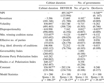
DEVDURit measures the deviation of the actual duration of a given cabinet from the predicted duration of the cabinet in a model with all control variables and the alternative measures of polarization. Negative values indicate overprediction, that is, the actual duration of a given cabinet was shorter than its predicted duration. Positive values indicate underprediction, that is, the government in question lasted longer than it should have given the model of Equation 8. We then regress the model given in Equation 5 on this measure of deviation. We perform the same operation on Equation 6, generating a predicted estimate of the number of cabinets and a measure of deviation (DEVNOGOVit) between the actual and predicted number of governments per electoral cycle. If our hypotheses hold, then NPI should have a significant positive effect on DEVDUR. In other words, high polarization should account for increasingly higher levels of underprediction of the null model of cabinet duration. Likewise, NPI should have a significant negative effect on DEVNOGOV.
Results
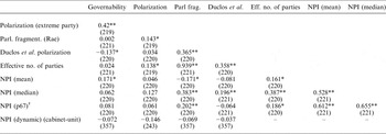
We start our discussion of the results by examining correlations between our measure of political polarization and other measures of dispersion/polarization used in the literature. Table 3 suggests that NPI has a positive and low (albeit statistically significant) correlation with the governability variable, as well as negative low correlations with the other measures of fragmentation/diversity commonly used in the literature to characterize the structure of the political system. These correlations are sufficiently low to suggest that our index of polarization is distinct from the other indexes that rely almost exclusively on the sizes of the parties or on the sizes of some exogenously determined subset of political parties. Thus, NPI appears to reflect a more general aspect of the bargaining environment in a given political system than alternative indices.Footnote 41
Correlations between the Network Polarization Index and Other Indices of Polarization/Dispersion

Notes: Numbers in parentheses are Ns.
†See fn. 29 for an explanation of ‘p67’.
*p < 0.05; **p < 0.01.
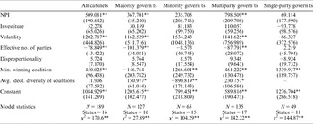
Table 4 tests our major hypotheses on election-cycle data. First, political polarization has a significant positive effect on duration in the general population of cases, as well as for majority cabinets and multiparty coalitions. However, in the case of minority or single-party cabinets, the effect of political polarization on cabinet duration is not statistically significant. As expected, political polarization plays an important role when it takes two or more parties to form a coalition or when the party or coalition in power controls a majority of the seats in parliament. Before discussing the differences in the key results across strata, let us examine the performance of the model on the number of cabinets in each electoral cycle.
Political Polarization and Cabinet Duration in European Parliaments

Notes: The values shown are time-series cross-sectional regression coefficients with correction for autocorrelation and overdispersion. Numbers in parentheses are robust standard errors.
*p < 0.05; **p < 0.01.
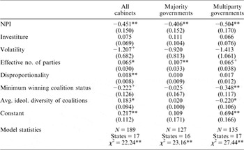
Table 5 omits the analysis of minority cabinets and single-party cabinets. In both cases, neither regression diagnostics nor any of the right-hand side variables were statistically significant. Yet in the general population, as well as in cases of multiparty coalitions and of majority cabinets, political polarization has a negative effect on the number of cabinets within an electoral cycle.
Political Polarization and Number of Cabinets per Electoral cycle in European Parliaments

Notes: The values shown are negative binomial time-series cross-sectional regression coefficients with correction for autocorrelation and overdispersion. Numbers in parentheses are robust standard errors.
+p < 0.10; *p < 0.05; **p < 0.01.
These results suggest that the polarization of the party system significantly impacts the political stability of parliamentary democracies given the multiparty coalitions or majority cabinets. However, in minority governments or single-party cabinets, the polarization of the political system does not significantly affect political stability. In such cases, the logic that drives the durability of cabinets is substantially different from the general majority and multiparty coalition cases. Our index of polarization is based on the extent to which parties take similar positions on the same issues. This defines both the composition of the cliques – proto-coalitions – and their cohesion. Single-party majority cabinets are typically a subset of one of the cliques. And while we have yet to investigate this, single-party majorities also form proper subsets of ‘optimal’ coalitions, that is, coalitions made up of ideologically similar parties that – given their size and cohesion – can form cohesive majorities. If that is the case, then our index can be modified to account for these situations, and this would strengthen our results considerably.
Minority cabinets represent a difficult nut to crack. The party or parties that form minority cabinets are possibly a subset of an optimal ideological coalition. Yet for reasons that require further inspection, they receive support from other ideologically similar parties that choose or are willing to stay outside the government. The duration of these cabinets, however, is significantly shorter than those of majority cabinets (F1, 220 = 21.08, p < 0.001).
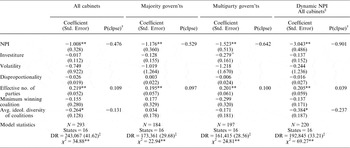
Next, we estimate the hazard of cabinet collapse using duration models. The unit of analysis is the individual cabinet. Here, we also use the interpolated NPI indices so that we have a time-varying estimate of political polarization. The results are given in Table 6.
Cabinet Durations in European Parliaments: Cox Proportional-Hazard Analysis

†Negative probabilities indicate reduced hazard of collapse.
‡DR = Days at risk (average years/state in parentheses).
§Dynamic NPI is NPI based on left–right position of parties, extrapolated over six-month intervals within electoral cycles.
+p < 0.1; *p < 0.05; **p < 0.01.
The results of Table 6 corroborate the results of the election-cycle unit of analysis. Using the original election-cycle NPI indices, we see that a one-unit increase in polarization reduces the hazard of cabinet collapse by nearly 42 per cent overall and by up to 62 per cent in the case of multiparty coalition governments. With the dynamic NPI index, the results appear to be even stronger: a unit increase in the polarization of a system just prior to the formation of a government reduces the hazard of government collapse by over 90 per cent. This suggests that our findings are robust not only with respect to the measurement of the key independent variable and to the measurement of the dependent variable but also to the unit of analysis used to measure cabinet duration.
A few words need to be said about the performance of the control variables in the analyses. None of the control variables consistently affects political stability, either in the electoral-cycle or in the cabinet unit of analysis. The minimum winning coalition measure has a positive effect on the average duration of majority and multiparty cabinets, but this effect disappears when we use the individual cabinet as the unit of analysis. Some of the controls significantly affect political stability but in the opposite direction from the expected one. For example, the volatility of electoral shifts shows a positive effect on government duration and reduces the hazard of cabinet collapse. Likewise, the ideological diversity of the coalition has a positive effect on cabinet duration, in contrast to the expectation that ideologically diverse cabinets are less likely to survive than ideologically cohesive ones. This suggests that most of the controls which have featured prominently in other studies of cabinet duration do not offer consistent insights into the stability of coalition systems. The interaction between political polarization and these variables needs to be studied in more detail in the future, but this is beyond the scope of the present study. We now turn to a comparison of the NPI and other measures of polarization. Table 7 provides the results of these tests.
Robustness Tests of NPI vis-à-vis Other Measures of Polarization

Note: Numbers in parentheses are robust standard errors.
+p < 0.10; *p < 0.05; **p < 0.01.
The results of this table corroborate our previous findings and suggest that NPI is robust with respect to other measures of polarization.Footnote 42 The effects of other measures of polarization on cabinet duration is either not robust or – in some cases – in the wrong direction. Moreover, NPI accounts for deviations of the actual duration of the cabinet from a predicted duration estimate. It also accounts – in the predicted direction – for deviations of the actual number of governments from the number predicted by a null model that contains alternative measures of polarization. This strengthens our confidence in our approach. Not only does the network polarization index significantly affect cabinet duration in general, but also it appears to explain some of the variance that is left unexplained by the more traditional measures of political polarization.
Conclusion
Many scholars have argued that the polarization of a party system affects democratic political stability. This article offers a number of contributions to this literature, beyond corroborating this argument. First, we offer a more general approach to the conceptualization and measurement of political polarization. This approach is based on the notion that the ideological structure of the party system along multiple dimensions forms an important foundation underlying the array of proto-coalitions. When these coalitions become discrete, internally cohesive and roughly equal in size, bargaining opportunities for individual parties decline. Consequently, the members of a coalition are ‘forced’ to manage political, economic, international and social crises within the same coalitional structure. As proto-coalitions are composed of overlapping parties and differ in size and cohesion, polarization declines and the system offers more bargaining opportunities to individual parties. Under such conditions, parties are more willing and able to defect from existing coalitions, thus either forming different cabinets under the same parliament, or calling for early elections.
Secondly, our measure of political polarization offers a more comprehensive and valid representation of this idea than previous measures of ideological or size-related dispersion. While it correlates with some of these measures, it is sufficiently different to suggest the viability and importance of an empirical analysis of the effect of polarization on cabinet duration. Our empirical results – while tentative in nature – offer sufficient evidence to suggest that additional research on polarization and political stability may yield more detailed insights into the process of cabinet formation and cabinet dissolution.
Thirdly, our empirical analyses on the effects of polarization on cabinet stability are more general and extensive than previous studies of the subject. We not only examine the effect of polarization, as we conceive this variable, on cabinet duration. We also conduct a number of robustness checks to test the sensitivity of our results to variation in measurement instruments (multiple measures of NPI), levels of analysis (cabinet level and electoral cycle level) and different conceptions of political polarization (comparison to other measures of the concept).
Finally, this study demonstrates the added value of Social Network Analysis to political processes in the comparative study of political systems. In many ways, SNA can add important insights, methodological innovations and substantive import to our understanding of politics as a set of complex relations among multiple actors. Our hope is that more political scientists would use and apply SNA models to study a wide variety of political phenomena and processes.
These contributions also suggest a number of possible extensions of this framework. In particular, it offers an opportunity to combine the attributes of the system – such as its level of political polarization – with the strategies and choices of individual parties in a better way. Hence, the next step in our project is to examine the relationship between the ‘optimality’ of a coalition and its stability. The ‘optimality’ concept incorporates the ideological distance of the parties making up the coalition, the ideological cohesiveness of the coalition, and its size. The interaction between system structure and network-related calculations of political parties will add a new impetus to the social choice modelling of coalition governments.
APPENDIX TABLE
Descriptive Statistics of Variables

*See fn. 29 for an explanation of ‘p67’.
APPENDIX: CONTROL VARIABLES
We employ a number of control variables that have been widely used in the cabinet duration literature to explain the survival of cabinets. These variables include:
Investiture (INVEST) is coded as 1 if an investiture vote is required for the approval of a cabinet and 0 otherwise. In the literature, the expectation has been that investiture should decrease cabinet durations.Footnote 43
Minimum Winning Coalition Index (MINWIN): This variable defines the extent to which a cabinet coalition deviates from the minimum winning size.Footnote 44 Deviations from the minimum winning status should decrease stability. Laver and Schofield, for instance, show that minority and surplus governments last a shorter period than do minimum winning cabinets.Footnote 45 We use two alternative measures, defined as:

where SEATSc is the sum of seats of the parties in the cabinet and PARLSEAT is the number of seats in the parliament. The first measure (MINWIN1) varies between −1 and +1 and takes into account the direction of deviation of the coalition from the minimum winning size. Thus, minority governments will get a negative score and majority governments will get a positive score. The second measure, MINWIN2, is the absolute deviation of the cabinet from the minimum winning size and varies between 0 and +1. The MINWIN scores are averaged across all cabinets within an electoral cycle.
Disproportionality (DISPROP): This index measures the discrepancy between the number of votes and the number of seats in a given political system and highly correlates with the electoral system of the country:Footnote 46

Disproportionality of systems suggests an endemic factor of imbalance that is considered to induce instability, thus leading to frequent government changes.
Volatility: Warwick defines this electoral volatility index as ‘one-half the sum of the proportional changes in parliamentary strengths of parties from one election to the next’.Footnote 47 It indicates the willingness of the voters to change their party allegiances from one election to the next. It is expected to decrease cabinet duration for two possible reasons. First, as King et al. state, electoral volatility indicates unstable bargaining environments. Secondly, following Strøm, we can argue that parties end coalitions sooner than later under high electoral volatility, because parties are concerned about losing even more votes in the next election. Being in government already costs governing parties votes, and if the electoral volatility is high, cabinets are expected to last a shorter time.Footnote 48
Effective Number of Parties: Warwick states that the effective number of parties is ‘an indicator of the complexity of the bargaining system in the parliament’ and therefore negatively affects cabinet formation and duration in West European countries.Footnote 49 The formula for the effective number of parties was first developed by Laakso and Taagepera:Footnote 50

,where seati is the seat share of each party within an election period.
Ideological Diversity of Coalition. We use the left–right index scores of parties in the CMP dataset for this measure. We calculate this measure as:

Where CD is the coalition ideological diversity, idi is the left–right score of party i, c indexes parties in the coalition, and n indexes parties in the parliament. This measure is the ratio of the standard deviation of the left–right scores of the parties in the coalition to the standard deviation of the left–right of all parties in the parliament. One expects that as CD increases, cabinet duration would decline. This measure is averaged for the election-cycle analyses, but it varies for each government when the government is the unit of analysis.Footnote 51
 where max|LR| is the width of the ideological range for this electoral cycle. Thus, sij is in the [0,1] range and higher values indicate strong ideological affinity between parties.