1 Introduction
Our interest in this study is with the stability of the vortex–wave interaction (VWI) states described by Hall & Smith (Reference Hall and Smith1989, Reference Hall and Smith1990, Reference Hall and Smith1991). The VWI approach provides a formal large Reynolds number asymptotic framework to describe numerically exact nonlinear solutions in shear flows. Such solutions have been found from a fully numerical approach by for example Nagata (Reference Nagata1990), Waleffe (Reference Waleffe2001), Wang, Gibson & Waleffe (Reference Wang, Gibson and Waleffe2007) and Gibson, Halcrow & Cvitanović (Reference Gibson, Halcrow and Cvitanović2009). The description of VWI given by Hall & Smith (Reference Hall and Smith1991) uncovered for the first time the tripartite interaction between inviscid waves, rolls and streaks, whilst the earlier asymptotic works by those authors described interactions associated with Tollmien–Schlichting waves. According to VWI theory, the waves exist as neutral disturbances to a streak flow and drive the rolls through their associated Reynolds stresses. This paper focuses on the stability of the inviscid type of VWI. For this type of interaction the waves are inviscid almost everywhere. However, crucially it turns out that the waves have most impact where they become viscous due to a singularity of the partial differential equation describing the inviscid wave system. The singularity occurs where the wave propagates downstream with the local fluid velocity and defines the location of a critical layer in which viscosity smooths out the singularity. The final link in the interaction is the driving of the streak by the roll field.
The simplicity of the interaction was clearly indicated by the relative scalings of the wave, roll and streak in Hall & Smith (Reference Hall and Smith1991), but since the theory was not applied to any particular shear flow until the work of Hall & Sherwin (Reference Hall and Sherwin2010), its existence was overlooked. Subsequently Waleffe (Reference Waleffe1997) uncovered the same tripartite interaction by an examination of the results from Navier–Stokes calculations and described it as a self-sustaining process. The VWI and self-sustaining process descriptions can, as shown in Hall & Sherwin (Reference Hall and Sherwin2010), be viewed as a steady streaming problem with the roll field established by the Reynolds stresses associated with the wave as it sloshes back and forth in a viscous critical layer which acts like a waveguide. Thus the origins of both approaches can be traced back to the description of steady streaming flows given by Stuart (1966) and more directly to a paper by Benney & Chow (Reference Benney and Chow1989) who speculated on possible mean flows driven by wave interactions.
Hall & Sherwin (Reference Hall and Sherwin2010) reproduced the numerical results of Wang et al. (Reference Wang, Gibson and Waleffe2007) with a high Reynolds number approach which turned out to give excellent agreement with Navier–Stokes calculations over a wide range of Reynolds numbers; see also Deguchi & Hall (Reference Deguchi and Hall2014) for a more complete account of the relationship between the results from the asymptotic approach and the full Navier–Stokes solutions. The advantage of the VWI approach is that the Reynolds number is scaled out of the problem and the three-dimensional unsteady Navier–Stokes problem is reduced to the solution of the two-dimensional Navier–Stokes equations at unit Reynolds number together with an advection diffusion equation and an inviscid partial differential equation eigenvalue problem.
The VWI system is difficult to handle numerically, since it involves a singularity and stress discontinuities at the critical layer. Thus the work of Hall & Sherwin (Reference Hall and Sherwin2010) was subsequently extended by Blackburn, Hall & Sherwin (Reference Blackburn, Hall and Sherwin2013) to a modified form where a hybrid approach can be employed to solve the VWI system. In the hybrid approach the terms in the Navier–Stokes equations which do not contribute to the leading-order VWI asymptotic approximation are ignored. Although the equations obtained in this way still depend on the Reynolds number, their asymptotic reduction gives the VWI system and their solution is readily used to extract the VWI solution. Thus the results computed using the hybrid approach are only meaningful when the results become independent of the sufficiently large ‘fictitious Reynolds number’. Having done careful asymptotic analysis to produce a Reynolds-number-independent problem it might at first sight seem like a backward step to then solve a computational problem involving it. However, the hybrid system is much simpler to solve numerically than both the VWI and full systems and a knowledge of its asymptotic solution is then readily used to extract the VWI solution from the numerical results. This approach proved superior to the original (Hall & Sherwin Reference Hall and Sherwin2010) regularisation procedure using delta functions. With this hybrid approach Blackburn et al. (Reference Blackburn, Hall and Sherwin2013) obtained VWI solutions over a wide range of wavenumbers establishing that VWI can exist in arbitrary shear flows with the disturbance energy of the wave satisfying Kolmogorov’s
 $5/3$
rule. Here we will use variations of the hybrid approach to solve the numerical problems associated with the three asymptotic regimes for the stability problem. The approach is of course only possible once the different regimes have been theoretically described and is again best viewed as perhaps the simplest way to derive the required constants appearing in the asymptotic theory.
At finite Reynolds number
 $R$
, nonlinear equilibrium solutions of the Navier–Stokes equations for the plane Couette flow configuration have been calculated by a number of authors. Results on the linear stability of such states have been given in, for example, Clever & Busse (Reference Clever and Busse1997), Nagata (Reference Nagata1998), Wang et al. (Reference Wang, Gibson and Waleffe2007), Gibson et al. (Reference Gibson, Halcrow and Cvitanović2009). These works repeatedly showed that all states have at least one unstable eigenvalue. As first found in Itano & Toh (Reference Itano and Toh2001), an interesting class of modes often referred to as lower-branch states can act as edge states which separate laminar and turbulent attractors. In Wang et al. (Reference Wang, Gibson and Waleffe2007) it was reported that the lower branch of solutions have a single unstable mode with growth rate which they estimated to scale like
 $R^{-0.48}$
as the Reynolds number was increased. This is the only unstable eigenmode the lower-branch state has, and it is the reason why the state acts as an edge state. In the full Navier–Stokes computational community similar stability studies have also been performed for various other shear flows, e.g. Pringle, Duguet & Kerswell (Reference Pringle, Duguet and Kerswell2009) for pipe flow, Okino et al. (Reference Okino, Nagata, Wedin and Bottaro2010) for square duct flow, Deguchi & Nagata (Reference Deguchi and Nagata2011) for sliding Couette flow. Despite the differences between the flow configurations, the trend of the stability results is uniform for these flows. For pipe flow Viswanath (Reference Viswanath2009) performed stability calculations of lower-branch states and found unstable eigenvalues that scaled like
 $R^{-0.41}$
and
 $R^{-0.87}$
.
Here we will describe the asymptotic structure of what turns out to be the three modes of instability of VWI states. Numerical verification of the theory will be provided using both the full Navier–Stokes equations and a hybrid approach to the stability problem motivated by Blackburn et al. (Reference Blackburn, Hall and Sherwin2013). In the next section we summarise the key points of the VWI description of equilibrium states in channel flows. In order to set the scene for our asymptotic analysis, we will in § 3 give results of Navier–Stokes computations of the stability of equilibrium coherent structures. The results suggest that, with time scaled on the channel depth divided by the wall speed, there are three types of eigenvalues with growth rates varying like
 $R^{0}$
,
 $R^{-1/2}$
and
 $R^{-1}$
. In § 4 we investigate the inviscid Rayleigh instability of equilibrium states which can produce unstable eigenvalues of order
 $R^{0}$
. Next, in § 5 we discuss what turns out to be a weak instability of the states operating on the diffusion time scale of the roll–streak flow. Since the mode operates on the diffusion time scale it is distributed across the entire flow and we will refer to it as the slow mode. In § 6 we consider a much more dangerous type of instability with the same streamwise wavenumber as the VWI state operating on a time scale between the slow roll–streak time scale and the Rayleigh instability time scale. The fact that this mode turns out to be the only unstable mode for most of the lower-branch equilibrium states for plane Couette flow leads directly to them being able to act as edge states. Finally, in § 7 some conclusions are drawn.
2 Vortex–wave interaction theory and some preliminary observations
We begin by summarising the principal equations describing VWI theory. For definiteness we focus on plane Couette flow, but the analysis is appropriate to any predominantly unidirectional shear flow. Our starting point is the momentum and continuity equations for an unsteady viscous flow of a fluid of constant density. Following the usual notation we take the Navier–Stokes equations in the form
 $$\begin{eqnarray}\displaystyle & \displaystyle (\unicode[STIX]{x2202}_{t}+\boldsymbol{u}^{\dagger }\boldsymbol{\cdot }\unicode[STIX]{x1D735})\boldsymbol{u}^{\dagger }=-\unicode[STIX]{x1D735}p^{\dagger }+{\displaystyle \frac{1}{R}}\unicode[STIX]{x1D6FB}^{2}\boldsymbol{u}^{\dagger }, & \displaystyle\end{eqnarray}$$
 $$\begin{eqnarray}\displaystyle & \displaystyle \unicode[STIX]{x1D735}\boldsymbol{\cdot }\boldsymbol{u}^{\dagger }=0. & \displaystyle\end{eqnarray}$$
 $\unicode[STIX]{x1D735}\equiv [\unicode[STIX]{x2202}_{x},\unicode[STIX]{x2202}_{y},\unicode[STIX]{x2202}_{z}]$
,
 $\boldsymbol{u}^{\dagger }=[u^{\dagger },v^{\dagger },w^{\dagger }]$
is the velocity,
 $p^{\dagger }$
is the pressure,
 $R$
is the Reynolds number and we will be interested in the limit
 $R\rightarrow \infty .$
The above equations are to be solved subject to
 $\boldsymbol{u}^{\dagger }=[\pm 1,0,0]$
at
 $y=\pm 1$
so that a basic plane Couette flow profile
 $\boldsymbol{u}^{\dagger }=[y,0,0]$
is a possible solution. At finite Reynolds numbers the above equations, beginning with Nagata (Reference Nagata1990), have been solved by a number of authors. We discuss only spanwise periodic solutions of the VWI equations having wavelength
 $2\unicode[STIX]{x03C0}/\unicode[STIX]{x1D6FD}$
. In the streamwise direction the solutions take the form of travelling waves with streamwise wavelength
 $2\unicode[STIX]{x03C0}/\unicode[STIX]{x1D6FC}$
and wave speed
 $c$
. In our numerical work the main focus is only on the stationary solutions, but the discussion we give is equally valid for the travelling wave case.
Our primary interest is in finding the large
 $R$
dependence of instabilities of equilibrium states. At high Reynolds numbers the roll–streak part of the flow depends on the slow diffusion time scale which is of size
 $O(R)$
whilst the wave must vary with an
 $O(1)$
time scale with time scaled on the half-channel width divided by the wall speed. We begin by writing
 $$\begin{eqnarray}\displaystyle & \displaystyle \boldsymbol{u}^{\dagger }=(U,R^{-1}V,R^{-1}W)+\cdots +R^{-7/6}(\boldsymbol{u}E+\text{C.C.})+\cdots , & \displaystyle\end{eqnarray}$$
 $$\begin{eqnarray}\displaystyle & \displaystyle p^{\dagger }=R^{-2}P+\cdots +R^{-7/6}(pE+\text{C.C.})+\cdots . & \displaystyle\end{eqnarray}$$
 $T=R^{-1}t$
is the slow diffusion time,
 $E=\exp [\text{i}\unicode[STIX]{x1D6FC}(x-R\int ^{T}c(T^{\prime })\,\text{d}T^{\prime })]$
, C.C. denotes complex conjugate and the only
 $x$
dependence of the flow is through
 $E$
so that
 $\boldsymbol{U}=[U,V,W]\in \mathbb{R}$
and
 $\boldsymbol{u}=[u,v,w]\in \mathbb{C}$
are functions of
 $y,z$
, and the slow time
 $T$
. The expansions (2.2) are carefully chosen to yield self-consistent non-trivial asymptotic equations at the large
 $R$
limit of Navier–Stokes equations. The
 $R^{-7/6}$
scaling of the wave is explained in detail in Hall & Smith (Reference Hall and Smith1991), Hall & Sherwin (Reference Hall and Sherwin2010) and is simply the size of the wave which can drive an
 $O(1)$
jump in the stresses of the roll field
 $(V,W)$
across the critical layer. Note also that the wave is locally neutral so
 $c$
is real for all time and, in view of the factor
 $R$
in the definition of
 $E$
, propagates down the channel with speed comparable to the wall speed. The relative scalings of the velocity components of the roll flow
 ${\sim}R^{-1}$
and the streak flow
 ${\sim}R^{0}$
and associated pressure
 ${\sim}R^{-2}$
are the usual ones for centrifugal instabilities in the small gap limit, or thin boundary layer limit, and were first identified by Taylor (Reference Taylor1923) in the context of the Taylor vortex problem.
We then derive
 $R$
-independent leading-order asymptotic equations for the roll–streak and wave components by substituting (2.2) into the Navier–Stokes equations (2.1). As expected, the equations of motion for the roll–streak flow are the viscous Taylor-vortex equations at zero Taylor number:
 $$\begin{eqnarray}\displaystyle & \displaystyle (\unicode[STIX]{x2202}_{\text{T}}+V\unicode[STIX]{x2202}_{y}+W\unicode[STIX]{x2202}_{z})\boldsymbol{U}=-(0,P_{y},P_{z})^{\text{T}}+\unicode[STIX]{x0394}\boldsymbol{U}, & \displaystyle\end{eqnarray}$$
 $$\begin{eqnarray}\displaystyle & \displaystyle \unicode[STIX]{x2202}_{y}V+\unicode[STIX]{x2202}_{z}W=0, & \displaystyle\end{eqnarray}$$
 $[U,V,W]=[\pm 1,0,0]$
at
 $y=\pm 1$
. Here
 $\unicode[STIX]{x1D6E5}=\unicode[STIX]{x2202}_{y}^{2}+\unicode[STIX]{x2202}_{z}^{2}$
is the two-dimensional Laplace operator. The wave drives the roll flow
 $V,W$
in the critical layer associated with the wave and leads to jump conditions in the derivatives of the quantities
 $V,W$
and the roll pressure
 $P$
across the layer; the detailed analysis of that jump will be given shortly. The asymptotic momentum and continuity equations for the wave can also be derived from the Navier–Stokes equations. These equations can be reduced to a single equation for the wave pressure. That equation describes the inviscid instability of streaks and was first given and solved in the context of Görtler vortices by Hall & Horseman (Reference Hall and Horseman1991); it takes the form
 $$\begin{eqnarray}\operatorname{div}\left({\displaystyle \frac{\unicode[STIX]{x1D735}(pE)}{(U-c)^{2}}}\right)=0.\end{eqnarray}$$
Equation (2.4) must be solved subject to the normal derivative of
 $p$
vanishing at any boundary; this condition ensures that the normal velocity of the wave vanishes at the wall, but a passive viscous wall layer must be inserted so that the no-slip conditions are satisfied. Henceforth, we will refer to the above equation as the generalised Rayleigh equation. So far, no equivalent of the inflection point theorem has been proved for this equation though it is readily shown that Howard’s semi-circle theorem is valid.
From (2.3), we see that as the slow time
 $T$
varies the roll then drives the streak flow
 $U$
whose stability properties to the wave are then altered thereby modifying the wave through (2.4). The modified wave then changes the jump conditions on the roll and the interaction between wave, roll and streak develops. The key feature of the interaction is that the
 $y,z$
components of the roll flow are
 $O(R^{-1})$
smaller than the streak. This describes a mechanism driving the roll flow which then couples through the streamwise momentum equation to the streak, thereby enabling asymptotically small waves to have an
 $O(1)$
effect back on the streak.
Now let us analyse the singularity of the wave equation (2.4). At the critical layer defined by
 $y=f(z,T)$
, where
 $U(f,z,T)=c(T)$
, the wave equation becomes singular. From the local analysis near the singular point we find that
 $u,v,w\backsim 1/(y-f)$
as the critical layer is approached. Thus in the critical layer the leading-order velocity components of the wave field are of size
 $R^{-7/6}\times R^{1/3}=R^{-5/6}$
since the critical layer is viscous and of thickness
 $R^{-1/3}$
. In order to find the form of the wave near the critical layer we need to determine the series form of the pressure as the layer is approached. This is most easily achieved by writing the wave pressure equation in terms of ‘body-fitted’ coordinates
 $(n,s)$
normal to and along the critical layer. We find that (2.4) becomes
 $$\begin{eqnarray}{\displaystyle \frac{\unicode[STIX]{x2202}^{2}p}{\unicode[STIX]{x2202}n^{2}}}+{\displaystyle \frac{\unicode[STIX]{x1D712}}{\mathscr{G}}}{\displaystyle \frac{\unicode[STIX]{x2202}p}{\unicode[STIX]{x2202}n}}+{\displaystyle \frac{1}{\mathscr{G}^{2}}}{\displaystyle \frac{\unicode[STIX]{x2202}^{2}p}{\unicode[STIX]{x2202}s^{2}}}-{\displaystyle \frac{\unicode[STIX]{x1D712}^{\prime }n}{\mathscr{G}^{3}}}{\displaystyle \frac{\unicode[STIX]{x2202}p}{\unicode[STIX]{x2202}s}}-\unicode[STIX]{x1D6FC}^{2}p-{\displaystyle \frac{2}{u-c}}\left({\displaystyle \frac{\unicode[STIX]{x2202}u}{\unicode[STIX]{x2202}n}}{\displaystyle \frac{\unicode[STIX]{x2202}p}{\unicode[STIX]{x2202}n}}+{\displaystyle \frac{1}{\mathscr{G}^{2}}}{\displaystyle \frac{\unicode[STIX]{x2202}u}{\unicode[STIX]{x2202}s}}{\displaystyle \frac{\unicode[STIX]{x2202}p}{\unicode[STIX]{x2202}s}}\right)=0,\end{eqnarray}$$
where
 $$\begin{eqnarray}\unicode[STIX]{x1D712}(s)={\displaystyle \frac{f_{zz}}{(1+f_{z})^{3/2}}}\end{eqnarray}$$
is the curvature of the critical layer, subscript
 $z$
denotes spanwise derivative and
 $\mathscr{G}=1+\mathscr{\unicode[STIX]{x1D712}}n$
. For convenience here and hereafter the dependence on the slow time
 $T$
is not displayed explicitly. In the vicinity of the critical layer
 $$\begin{eqnarray}u-c=\unicode[STIX]{x1D706}_{1}(s)n+\unicode[STIX]{x1D706}_{2}(s)n^{2}+\cdots\end{eqnarray}$$
and the Frobenius expansion of the wave pressure equation for small positive
 $n$
takes the form
 $$\begin{eqnarray}p=p_{0}(s)+p_{2}(s)n^{2}+p_{3L}(s)n^{3}\ln n+p_{3}(s)n^{3}+\cdots .\end{eqnarray}$$
Here
 $p_{0}$
and
 $p_{3}$
are functions of
 $s$
fixed by the conditions at the walls and all other coefficients can be determined by these functions. For example,
 $$\begin{eqnarray}\displaystyle & \displaystyle p_{2}={\displaystyle \frac{1}{2}}\left[p_{0}^{\prime \prime }-2{\displaystyle \frac{\unicode[STIX]{x1D706}_{1}^{\prime }}{\unicode[STIX]{x1D706}_{1}}}p_{0}^{\prime }-\unicode[STIX]{x1D6FC}^{2}p_{0}\right], & \displaystyle\end{eqnarray}$$
 $$\begin{eqnarray}\displaystyle & \displaystyle p_{3L}={\displaystyle \frac{1}{3}}\left[\left({\displaystyle \frac{4\unicode[STIX]{x1D706}_{2}}{\unicode[STIX]{x1D706}_{1}}}-2\unicode[STIX]{x1D712}\right)p_{2}+2\unicode[STIX]{x1D712}p_{0}^{\prime \prime }+\unicode[STIX]{x1D712}^{\prime }p_{0}^{\prime }+{\displaystyle \frac{2\unicode[STIX]{x1D706}_{1}^{\prime }}{\unicode[STIX]{x1D706}_{1}}}\left({\displaystyle \frac{\unicode[STIX]{x1D706}_{2}^{\prime }}{\unicode[STIX]{x1D706}_{1}^{\prime }}}-{\displaystyle \frac{\unicode[STIX]{x1D706}_{2}}{\unicode[STIX]{x1D706}_{1}}}-2\unicode[STIX]{x1D712}\right)p_{0}^{\prime }\right]. & \displaystyle\end{eqnarray}$$
The asymptotic structure of the wave in the critical layer is the usual viscous critical layer one so that in the neutral case, the logarithm transforms in the usual way
 $$\begin{eqnarray}\displaystyle \ln n=\ln |n|-\text{i}\unicode[STIX]{x03C0}\,\text{sgn}(\unicode[STIX]{x1D706}_{1})\quad \text{if }n<0. & & \displaystyle\end{eqnarray}$$
Thus if we write an expansion similar to (2.8) for negative
 $n$
, replacing
 $\ln n$
by
 $\ln |n|$
,
 $p_{3}$
suffers a jump
 $\text{i}\unicode[STIX]{x03C0}p_{3L}$
across the critical layer. In the papers by Brown et al. (Reference Brown, Brown, Smith and Timoshin1993) and Blackaby & Hall (Reference Blackaby and Hall1995) the assumption was made that the logarithmic term should be suppressed. However, it is important to notice that there is no reason why the coefficient of the logarithmic term in the series expansion of the wave pressure should vanish. If we try to force the term to vanish then the above equation specifies
 $\unicode[STIX]{x1D6FC}$
as an eigenvalue, which is not possible since the value of
 $\unicode[STIX]{x1D6FC}$
has already been fixed. Furthermore the numerical solutions of Hall & Sherwin (Reference Hall and Sherwin2010) suggest that, in general, the logarithm does not vanish; notice that if there is no logarithmic term we can transform
 $p$
to be purely real by multiplying by a complex constant. An exception occurs when the critical layer is flat, as is the case for some solutions in plane Couette flow; see EQ7/EQ8 in Gibson et al. (Reference Gibson, Halcrow and Cvitanović2009). This case corresponds to
 $\unicode[STIX]{x1D712}=\unicode[STIX]{x1D706}_{2}=0$
where there is no logarithmic term in the Frobenius expansion, and is mathematically very similar to the upper-branch neutral modes of inflectional unidirectional flows depending on one spatial variable.
Whether or not there is a logarithmic term has no influence on the leading-order problem, although it plays a role in § 6. Following the discussion given in Hall & Sherwin (Reference Hall and Sherwin2010), the jump conditions for the roll are most succinctly expressed in terms of the roll stresses along and normal to the critical layer. If we denote the component of the roll velocity field
 $(V,W)$
resolved in the
 $s$
direction by
 $V^{s}(n,s)$
then it can be shown that the following jumps are to be applied across the critical layer:
 $$\begin{eqnarray}\displaystyle \left[{\displaystyle \frac{\unicode[STIX]{x2202}V^{s}}{\unicode[STIX]{x2202}n}}\right]_{-}^{+}=n_{0}\unicode[STIX]{x1D6FC}^{-5/3}{\displaystyle \frac{\text{d}Q}{\text{d}s}}\equiv J(s),\quad \left[P\right]_{-}^{+}=-n_{0}\unicode[STIX]{x1D6FC}^{-5/3}\unicode[STIX]{x1D712}Q\equiv K(s), & & \displaystyle\end{eqnarray}$$
where
 $$\begin{eqnarray}Q=\unicode[STIX]{x1D706}_{1}^{-5/3}\left|{\displaystyle \frac{\unicode[STIX]{x2202}p_{0}}{\unicode[STIX]{x2202}s}}\right|^{2},\quad n_{0}=2\unicode[STIX]{x03C0}\left({\displaystyle \frac{2}{3}}\right)^{2/3}\left(-{\displaystyle \frac{2}{3}}\right)!,\end{eqnarray}$$
and
 $p_{0}(s)$
is as defined in (2.8). These equations are derived by considering the viscous roll equations in the critical layer in the presence of the Reynolds stress of the wave. The Reynolds stress term is associated with the self-interaction of the wave. Thus its size is the square of the wave amplitude in the critical layer multiplied by the critical layer thickness, i.e.
 $R^{-5/3}\times R^{-1/3}$
. As expected, this balances to the size of the roll viscous term,
 $R^{-2}$
. Note that in Hall & Sherwin (Reference Hall and Sherwin2010), in order to quantify the size of the wave field, the wave pressure was normalized and an
 $O(1)$
amplitude introduced. We make no such normalisation here so that the above expressions differ slightly from those given in that paper.
We are now in a position to summarize the effect of the wave on the roll–streak. Firstly we note that the roll equations, i.e.
 $y$
,
 $z$
components of (2.3a
), are to be solved subject to the no-slip conditions at any boundary. At the critical layer, the velocity components
 $V,W$
are continuous but the roll stresses must satisfy the jump conditions (2.12)–(2.13). The jump conditions are functions of the wave pressure eigenfunction
 $p$
evaluated on the critical layer, but parameterized in terms of
 $(n,s)$
rather than
 $(y,z)$
. Having determined the roll velocity, the streak velocity follows from the streamwise component of (2.3a
) which is to be solved subject to no slip at any boundary. The pressure eigenfunction
 $p$
must then satisfy (2.4), which then closes the VWI system for the roll, streak and wave.
At first sight the pressure equation looks linear but in fact
 $U$
depends on
 $p$
through
 $V,W$
so the equation is indeed nonlinear. If we assume all quantities are known at an instant
 $T$
, then the equations must be stepped forward in time in such a way that the updated pressure satisfies (2.4) at the new time step and
 $c$
must remain real. This is achieved by suitably varying the overall amplitude of the wave. Travelling wave solutions of the interaction equations correspond to the solutions being independent of
 $T$
and we concern ourselves here with the instability of those solutions. For plane Couette flow, most of the known solutions are stationary so that
 $c=0$
but our discussion below will apply to the more general case when it is non-zero.
Results given by Hall & Sherwin (Reference Hall and Sherwin2010), Blackburn et al. (Reference Blackburn, Hall and Sherwin2013), Deguchi & Hall (Reference Deguchi and Hall2014) for plane Couette flow correspond to a stationary mode so that
 $c=0$
and we will restrict our results to that case. This mode is a high Reynolds number extension of those of Nagata (Reference Nagata1990), Wang et al. (Reference Wang, Gibson and Waleffe2007), EQ1/EQ2 in Gibson et al. (Reference Gibson, Halcrow and Cvitanović2009) and has the symmetries
 $$\begin{eqnarray}\displaystyle & \displaystyle [u^{\dagger },v^{\dagger },w^{\dagger }](x,y,z)=[u^{\dagger },v^{\dagger },-w^{\dagger }](x+\unicode[STIX]{x03C0}/\unicode[STIX]{x1D6FC},y,-z), & \displaystyle\end{eqnarray}$$
 $$\begin{eqnarray}\displaystyle & \displaystyle [u^{\dagger },v^{\dagger },w^{\dagger }](x,y,z)=[-u^{\dagger },-v^{\dagger },w^{\dagger }](-x,-y,z+\unicode[STIX]{x03C0}/\unicode[STIX]{x1D6FD}). & \displaystyle\end{eqnarray}$$
 $R$
dependence using the known scalings for VWI states. The resultant formulation is essentially the hybrid approach of Blackburn et al. (Reference Blackburn, Hall and Sherwin2013) with a minor difference which will be elucidated in the next section. For a fixed spanwise wavenumber
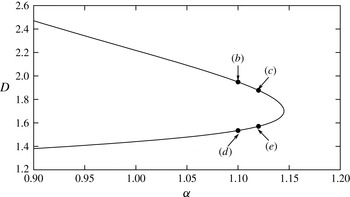
 $\unicode[STIX]{x1D6FD}$
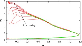
the VWI states occur as upper and lower-branch states connected through a saddle-node bifurcation as seen in figure 1. The solutions shown were found using the code developed in Deguchi, Hall & Walton (Reference Deguchi, Hall and Walton2013). Excellent convergence can be seen for both the upper and lower branches, and the results are in agreement at large Reynolds numbers with the fully resolved Navier–Stokes computations given by Deguchi & Hall (Reference Deguchi and Hall2014). Note that, as discussed in Deguchi & Hall (Reference Deguchi and Hall2014), the approach to the VWI curve becomes relatively slow on the upper branch as the wavenumber decreases. Typically on the lower branch and the upper branch close to the saddle node a Reynolds number of order 10 000 will suffice whilst the point at the left-hand end of the upper branch in figure 1 needs much larger values of
 $R$
for convergence.
The drag
 $D$
on the lower wall for the steady solutions with
 $\unicode[STIX]{x1D6FD}=2$
as a function of the streamwise wavenumber
 $\unicode[STIX]{x1D6FC}$
. The thin red curves correspond to the equilibrium solutions for
 $R=10^{4},2\times 10^{4},4\times 10^{4}$
and
 $6\times 10^{4}$
with only the first streamwise Fourier mode taken. The points indicated by ▵,
 $\times$
and ○ are similar results for
 $R=10^{5},2\times 10^{5}$
and
 $8\times 10^{5}$
, respectively. The green thick dashed curve is the fully resolved solution for
 $R=4\times 10^{4}$
, computed in Deguchi & Hall (Reference Deguchi and Hall2014). The solutions above/below the saddle-node point are referred to as the upper and lower-branch solutions respectively.

3 Stability results at finite Reynolds numbers using the linearised Navier–Stokes equations
Here we consider the linear instability of finite Reynolds number equilibrium states using the Navier–Stokes equations linearised around the equilibrium states. The numerical scheme used is described in Deguchi et al. (Reference Deguchi, Hall and Walton2013). We will use the finite Reynolds number results to suggest possible high Reynolds number dependencies for disturbances to VWI states. We will see that the calculations suggest three types of asymptotic structures for disturbances to VWI states. The stability problem is formulated by perturbing an equilibrium solution
 $[u^{\dagger },v^{\dagger },w^{\dagger }]=[\overline{u}^{\dagger },\overline{v}^{\dagger },\overline{w}^{\dagger }]$
of (2.1) subject to plane Couette flow boundary conditions to a disturbance of the same spanwise and streamwise wavelengths as the equilibrium state. Thus we write
 $$\begin{eqnarray}[u^{\dagger },v^{\dagger },w^{\dagger }]=[\overline{u}^{\dagger },\overline{v}^{\dagger },\overline{w}^{\dagger }]+\unicode[STIX]{x1D6FF}[\widetilde{u}^{\dagger },\widetilde{v}^{\dagger },\widetilde{w}^{\dagger }]\text{e}^{\unicode[STIX]{x1D70E}t},\end{eqnarray}$$
where
 $\unicode[STIX]{x1D6FF}$
is an infinitesimally small disturbance amplitude and
 $\unicode[STIX]{x1D70E}=\unicode[STIX]{x1D70E}_{r}+\text{i}\unicode[STIX]{x1D70E}_{i}$
is a complex growth rate. In (3.1) terms proportional to
 $\text{e}^{\unicode[STIX]{x1D70E}^{\ast }t}$
, where
 $\ast$
represents complex conjugate, must be added to construct the real flow field, but we omit such terms for the sake of simplicity. For computational purposes the velocities are expressed in a potential form, and then discretized using truncated Fourier and Chebyshev expansions. The eigenvalues of the discretized linear system describing the linearised stability problem can be found using a direct linear solver or Arnoldi method. Less restricted disturbances such as different streamwise wavelengths could be found using Floquet theory, as considered in Clever & Busse (Reference Clever and Busse1997), Nagata (Reference Nagata1998) for example, but that is not attempted here.
We now examine the large Reynolds number behaviour of the eigenvalues near the saddle-node point where the full Navier–Stokes equilibrium solution exhibits good convergence to the VWI curve. We concentrate on the spanwise wavenumber
 $\unicode[STIX]{x1D6FD}=1.667$
which corresponds to the minimal box size needed to sustain turbulence; see Hamilton, Kim & Waleffe (Reference Hamilton, Kim and Waleffe1995). For this wavenumber, the trend of the VWI convergence is similar to the case
 $\unicode[STIX]{x1D6FD}=2$
which we discussed in the last section. At a given Reynolds number we consider the stability of the solution appropriate to different points on the bifurcation diagram. As seen for example in Gibson et al. (Reference Gibson, Halcrow and Cvitanović2009), typically there is one relatively small unstable eigenvalue for the lower-branch solutions and there are several large unstable eigenvalues for the upper-branch solutions. The most dangerous eigenvalues typically have the symmetries (2.14a
)–(2.14b
), so in this study we restrict our attention to this symmetric subspace. Notice that this restriction excludes the possibility of zero eigenvalues associated with translational invariance of the system in
 $x$
and
 $z$
. Having found the most unstable eigenvalues well away from the saddle-node point we then examine how those eigenvalues found for the upper and lower branches vary with
 $\unicode[STIX]{x1D6FC}$
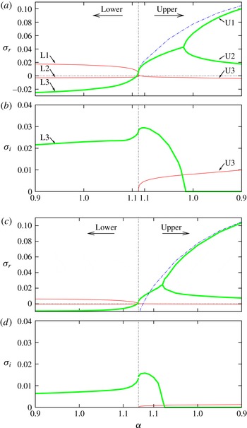
. Figure 2 shows growth rates continued from the most unstable modes for the equilibrium state for
 $R=3000$
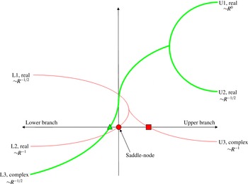
and 20 000. The thin red and thick green curves respectively show a family of eigenvalues connecting the most unstable eigenvalues of the lower and upper branches away from the saddle-node point; other less unstable eigenvalues exist but these are not shown for the sake of simplicity. Notice that in the figures the solution branch is unfolded at the saddle-node point so that the left/right half of the figures represent the stability of the lower/upper branch respectively. The eigenvalues reconnect when they approach the saddle-node point; see the schematic picture figure 3. The saddle-node point for
 $\unicode[STIX]{x1D6FD}=1.667$
is at
 $\unicode[STIX]{x1D6FC}\approx 1.1$
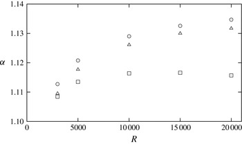
but it is weakly dependent on
 $R$
as indicated by circles in figure 4. Notice that the slightly larger value of
 $\unicode[STIX]{x1D6FC}=1.14$
corresponds to the minimal flow unit introduced by Hamilton et al. (Reference Hamilton, Kim and Waleffe1995).
The real and imaginary parts of the selected eigenvalues along the equilibrium solution branch for
 $\unicode[STIX]{x1D6FD}=1.667$
. Full linearised Navier–Stokes computations are used, and the wavenumbers and symmetries of the perturbation are restricted to those of the equilibrium state. (a,b)
 $R=3000$
. (c,d)
 $R=20\,000$
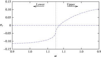
. The dotted vertical line indicates the position of the saddle-node point, and the left/right parts of the figures show the stability of the lower/upper equilibrium solution branches. The thin red and thick green curves indicate families of eigenvalues which connect to the most amplified modes on the lower/upper equilibrium solution curve. The blue dot-dashed curves correspond to the Rayleigh stability results shown later in figure 9.

Schematic of the connection of the eigenvalues seen in figure 2. The horizontal and vertical axes represents
 $\unicode[STIX]{x1D6FC}$
and
 $\unicode[STIX]{x1D70E}_{r}$
, respectively.

The Reynolds number dependence of the neutral points associated with L2 (○), L3 (▵) and U3 (▫); see figure 3. Notice that ○ also represents the position of the saddle node.

For the lower-branch results in figure 2, the thin red curves correspond to real growth rates, and one is stable whilst the other is unstable. We label these modes as L1 and L2, respectively; see figure 3. The thick green curve beneath the L2 branch corresponds to a stable complex eigenvalue which is labelled L3 and becomes unstable just before the saddle-node point shown by the vertical dotted line. After becoming unstable, the growth rate continues to increase as the upper branch is traversed. Then, at a point on the upper branch, the complex conjugate pair of eigenvalues splits into two real ones. Subsequently, one of the growth rates grows whilst the other decreases. These modes are labelled as U1 and U2, respectively. The L2 eigenvalue at the lower branch passes through neutrality at exactly the saddle-node point before meeting the L1 eigenvalue on the upper branch. After meeting, the eigenvalues generate a complex conjugate pair of unstable modes which then pass through neutrality at a point on the upper branch; we label this mode as U3. Notice that now it is clear that the modes with non-zero
 $\unicode[STIX]{x1D70E}_{i}$
seen in figure 2 correspond to L3 and U3. We will comment later on the significance of the blue dot-dashed curve shown in figure 2.
Comparison of the results over a range of Reynolds numbers shows that the positions where the L3 and U3 eigenvalues pass through neutrality are close to the saddle-node point but on the upper and lower branches respectively. An important point to note in figure 4 is that the points do not approach the saddle node when
 $R$
increases indefinitely. We conclude then that when
 $R$
increases, there are three neutral points near the saddle node of the solution branch, corresponding to L3, L2, U3. The neutral point associated with L2 is an obvious eigenvalue arising at the saddle-node point. The other two neutral points have imaginary parts which can be inferred from the lower plots of figure 2(b,d). In that figure we observe that the frequency of L3 is much higher than that of U3.
Now let us analyse the Reynolds number scaling of the eigenvalues at
 $\unicode[STIX]{x1D6FC}=1$
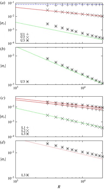
; results for the upper and lower branches are shown in figure 5. First figure 5(c,d) shows that real part of the growth rates of the unstable L1 and stable L3 eigenvalues on the lower branch vary approximately like
 $R^{-1/2}$
for large
 $R$
. Likewise figure 5(a,b) shows that real parts of the U2 eigenvalues on the upper branch vary approximately like
 $R^{-1/2}$
. The solid red lines in the figures have slope
 $-1/2$
and correspond to results from the asymptotic discussion to be given in § 6. However, notice that the dotted red line in figure 5(d) has a smaller slope close to
 $-5/8$
and suggests that the L3 eigenvalues have frequency proportional to
 $R^{-5/8}$
.
The Reynolds number scaling of the eigenvalues for
 $\unicode[STIX]{x1D6FC}=1$
. The blue dot-dashed line
 ${\sim}R^{0}$
is the Rayleigh mode hybrid computation result to be discussed in § 4. The green dashed line
 ${\sim}R^{-1}$
is the slow mode hybrid computation result to be discussed in § 5. The red solid line
 ${\sim}R^{-1/2}$
is the edge mode hybrid computation result to be discussed in § 6. The red dotted line has a slope
 $-5/8$
. (a,b) Upper-branch equilibrium solution. (c,d) Lower-branch equilibrium solution.

Figure 5(a,b) shows clearly that the real unstable eigenvalue U1 for the upper branch is almost independent of the Reynolds number. The blue dot-dashed line is a line of zero slope and predicted by our analysis in § 4 of the stability properties of the streak part of the VWI state.
Finally, the real parts of the L2 and U3 eigenvalues are found to scale approximately like
 $R^{-1}$
for large
 $R$
. Note here that the green dashed curves in the plots have slope
 $-1$
and correspond to the asymptotic analysis to be given in § 5.
The above results suggest that there are at least three time scales on which modes operate. The two extremes are readily identified. Firstly the mode on the upper-branch scaling like
 $R^{0}$
is most likely a Rayleigh instability of the streak. The mode operating on the
 $R^{-1}$
time scale occurs on the time scale on which roll–streak flows evolve within the VWI formulation. Therefore, we can anticipate that it is a mode of instability accessible directly from the VWI equations. The intermediate scale eigenvalue of order
 $R^{-1/2}$
has a similar scaling to the
 ${\sim}R^{-0.48}$
inferred from numerical calculations by Wang et al. (Reference Wang, Gibson and Waleffe2007). The origin of the mode on the intermediate time scale is not obvious at this stage but, since it corresponds to the single unstable mode associated with edge states, we will refer to it as the edge mode. We therefore suggest that the three types of modes operational in the stability problem of equilibrium states:
-
(i) Rayleigh modes are instabilities of the streak part of the VWI states and at leading order are not influenced by the roll and wave of the VWI state as will be shown in the next section. They simply produce rapidly growing Rayleigh modes which would quickly swamp the VWI state.
-
(ii) Slow modes are rather ponderous modes operating on the time scale of order
 $R$
on which the roll and streak part of the VWI state evolve. We will see in § 5 that they correspond to modulations of the VWI state with the critical layer being perturbed as well as the wave, roll and streak of the underlying VWI state.
-
(iii) Edge modes correspond to neutral Rayleigh waves perturbed into the unstable regime by higher-order effects. We discuss these modes in § 6 and show that the time scale of the modes scales like
$R^{1/2}$
. Here we will see that the instability takes on the form of an inviscid roll–streak perturbation in the majority of the channel, and that viscous effects are concentrated around the critical layer which has its leading-order position unperturbed.


In the later sections we will develop asymptotic theories for the three types of modes mentioned above. The numerical evaluations of the coefficients of the eigenvalues in the different expansions turn out to be themselves formidable challenges. Following in the spirit of Blackburn et al. (Reference Blackburn, Hall and Sherwin2013) we will extract those coefficients by generating hybrid stability problems having equivalent leading-order asymptotic forms for the eigenvalues that govern the stability. With that in mind we now discuss a particular hybrid stability problem.
We saw in § 2 that the generalised Rayleigh equation satisfied by the wave pressure of the VWI problem has a singularity at the critical layer and leads to jumps in the stresses of the outer roll flow occur. Thus in order to determine the asymptotic scales of the modes alluded to above, for the first instance we simply consider a linear stability of the hybrid problem discussed by Blackburn et al. (Reference Blackburn, Hall and Sherwin2013) with a fictitious Reynolds number
 $R=R_{f}.$
In fact the asymptotic eigenvalues can be extracted by making minor modifications to the full Navier–Stokes eigenvalue problem of this section. The hybrid problem of Blackburn et al. (Reference Blackburn, Hall and Sherwin2013) proceeds by first restricting the streamwise dependence to be proportional to a Fourier mode with wavenumbers
 $\pm \unicode[STIX]{x1D6FC}$
. Thus we substitute
 $$\begin{eqnarray}\displaystyle \left.\begin{array}{@{}c@{}}\displaystyle \overline{\boldsymbol{u}}^{\dagger }=\overline{\boldsymbol{U}}(y,z)+\{\overline{\boldsymbol{u}}(y,z)E+\text{C.C.}\},\quad \overline{p}^{\dagger }=\overline{P}(y,z)+\{\overline{p}(y,z)E+\text{C.C.}\},\\ \displaystyle \widetilde{\boldsymbol{u}}^{\dagger }=\widetilde{\boldsymbol{U}}(y,z)+\{\widetilde{\boldsymbol{u}}(y,z)E+\text{C.C.}\},\quad \widetilde{p}^{\dagger }=\widetilde{P}(y,z)+\{\widetilde{p}(y,z)E+\text{C.C.}\},\end{array}\right\} & & \displaystyle\end{eqnarray}$$
into (3.1), in order to find the hybrid stability equations. At
 $O(\unicode[STIX]{x1D6FF}^{0})$
, the part denoted by an overline satisfies the Navier–Stokes equations with a streamwise Fourier expansion truncated at the first mode. Although the formulation derived in this way correctly captures the VWI equilibrium solutions, as shown in § 2, we further need to eliminate some terms to recover the hybrid problem of Blackburn et al. (Reference Blackburn, Hall and Sherwin2013). This is because from the generalized Rayleigh equation we can see that the wave part is only influenced by the streak and the roll field does not play any role. Eliminating such roll–wave interaction terms from the
 $x$
-dependent part of the numerical code used in this and the last sections, we recover the same framework as Blackburn et al. (Reference Blackburn, Hall and Sherwin2013) but with a Newton method rather than successive fixed point iterations of roll, streak and wave solver. In the hybrid computation the roll flow subject to the jumps is solved by inserting the Reynolds stress from the interaction of the waves. Likewise the generalized Rayleigh equation is solved by replacing to the Navier–Stokes equations linearised around
 $[\overline{U},0,0]$
.
Suppose that we have a nonlinear equilibrium solution of the hybrid problem at some fictitious Reynolds number
 $R=R_{f}$
with streamwise and spanwise wavenumbers
 $\unicode[STIX]{x1D6FC}$
and
 $\unicode[STIX]{x1D6FD}$
, respectively. Then at
 $O(\unicode[STIX]{x1D6FF})$
in the perturbed hybrid equations we have the stability equations, which are formed by the roll–streak part
 $$\begin{eqnarray}\displaystyle & \hspace{-20.00003pt}\displaystyle (\unicode[STIX]{x1D70E}+\{\overline{V}\unicode[STIX]{x2202}_{y}+\overline{W}\unicode[STIX]{x2202}_{z}\}-R_{f}^{-1}\unicode[STIX]{x1D6E5})\left[\begin{array}{@{}c@{}}\widetilde{U}\\ \widetilde{V}\\ \widetilde{W}\end{array}\right]+(\widetilde{V}\unicode[STIX]{x2202}_{y}+\widetilde{W}\unicode[STIX]{x2202}_{z})\left[\begin{array}{@{}c@{}}\overline{U}\\ \{\overline{V}\}\\ \{\overline{W}\}\end{array}\right]+\left[\begin{array}{@{}c@{}}0\\ \widetilde{P}_{y}\\ \widetilde{P}_{z}\end{array}\right]=\text{R.S.}, & \displaystyle\end{eqnarray}$$
 $$\begin{eqnarray}\displaystyle & \hspace{-20.00003pt}\displaystyle \unicode[STIX]{x2202}_{y}\widetilde{V}+\unicode[STIX]{x2202}_{z}\widetilde{W}=0, & \displaystyle\end{eqnarray}$$
and the wave part
 $$\begin{eqnarray}\displaystyle & & \displaystyle (\{\unicode[STIX]{x1D70E}\}+\text{i}\unicode[STIX]{x1D6FC}(\overline{U}-c)-R_{f}^{-1}(\unicode[STIX]{x1D6E5}-\unicode[STIX]{x1D6FC}^{2}))\left[\begin{array}{@{}c@{}}\widetilde{u}\\ \widetilde{v}\\ \widetilde{w}\end{array}\right]+\text{i}\unicode[STIX]{x1D6FC}\widetilde{U}\left[\begin{array}{@{}c@{}}\overline{u}\\ \overline{v}\\ \overline{w}\end{array}\right]\nonumber\\ \displaystyle & & \displaystyle \quad +\,(\widetilde{v}\unicode[STIX]{x2202}_{y}+\widetilde{w}\unicode[STIX]{x2202}_{z})\left[\begin{array}{@{}c@{}}\overline{U}\\ 0\\ 0\end{array}\right]+(\overline{v}\unicode[STIX]{x2202}_{y}+\overline{w}\unicode[STIX]{x2202}_{z})\left[\begin{array}{@{}c@{}}\widetilde{U}\\ 0\\ 0\end{array}\right]+\left[\begin{array}{@{}c@{}}\text{i}\unicode[STIX]{x1D6FC}\widetilde{p}\\ \unicode[STIX]{x2202}_{y}\widetilde{p}\\ \unicode[STIX]{x2202}_{z}\widetilde{p}\end{array}\right]=0,\end{eqnarray}$$
 $$\begin{eqnarray}\displaystyle \text{i}\unicode[STIX]{x1D6FC}\widetilde{u}+\unicode[STIX]{x2202}_{y}\widetilde{v}+\unicode[STIX]{x2202}_{z}\widetilde{w}=0. & & \displaystyle\end{eqnarray}$$
Here R.S. describes the Reynolds stress produced by the interaction of
 $\overline{\boldsymbol{u}}$
and
 $\widetilde{\boldsymbol{u}}$
. The eigenvalue problem proposed above have eigenvalues
 $\unicode[STIX]{x1D70E}$
of different asymptotic behaviour in
 $R_{f}$
, and thus the corresponding eigenfunctions have a different asymptotic structure. Therefore, for each mode, we further need to eliminate several terms from (3.3), to construct a regularised problem which in the limit gives the correct asymptotic forms suitable for the different stability modes. As we shall see in the following sections, the terms in the curly brackets in (3.3a
) and (3.3c
) are of relevance for that elimination process. Throughout the rest of the paper the fictitious Reynolds number is chosen as
 $R_{f}=30\,000$
. That choice is reasonable as long as we do not investigate small
 $\unicode[STIX]{x1D6FC}$
upper-branch states; see figure 2.
4 Rayleigh mode instabilities of VWI equilibrium streaks
We recall that a VWI state is a roll–streak flow driven by the Reynolds stresses associated with a wave propagating on the streak. The wave is inviscid apart from the critical layer where it drives the roll and in the passive side wall viscous layers. Most important though is the fact that the wave and roll are asymptotically small compared to the streak. Thus any inviscid wave superimposed on the VWI structure will satisfy the generalized Rayleigh equation (2.4) with the equilibrium streak as the background flow. Now we let
 $\widetilde{\unicode[STIX]{x1D6FC}}$
and
 $\widetilde{c}$
denote the wavenumber and wave speed of an arbitrary perturbation to the VWI flow; note that there is no reason why we should choose the disturbance to have the same wavenumber and phase speed as the equilibrium VWI state. In this section, for the sake of clarity, we denote the wavenumber and wave speed of the equilibrium state by
 $(\overline{\unicode[STIX]{x1D6FC}},\overline{c})$
.
In most of the literature regarding the instability based on Navier–Stokes computations, the streamwise wavenumber of perturbations has been fixed to be that of the nonlinear equilibrium solution. That assumption immediately rules out the most dangerous route for a nonlinear state to be destroyed. Although confirmation of these results is possible if the computational domain of the simulations is selected to be the same as that of the stability problem, flows in the real world are less inhibited about the wavenumber selected. Therefore the excluded modes might actually be the most important in practice. Paradoxically the instability of VWI states to this possibly most important class of mode is the easiest to consider.
Suppose then that we have a stationary equilibrium solution of the VWI system determined by (2.3a ), (2.4) and (2.12). If the roll, streak and wave part of that equilibrium state are denoted by an overline, let us now perturb it by writing
 $$\begin{eqnarray}\displaystyle & \displaystyle \boldsymbol{u}^{\dagger }=(\overline{U},R^{-1}\overline{V},R^{-1}\overline{W})+\cdots +R^{-7/6}\{(\overline{\boldsymbol{u}}\overline{E}+\unicode[STIX]{x1D6FF}\widetilde{\boldsymbol{u}}\widetilde{E})+\text{C.C.}\}+\cdots , & \displaystyle\end{eqnarray}$$
 $$\begin{eqnarray}\displaystyle & \displaystyle p^{\dagger }=R^{-2}\overline{P}+\cdots +R^{-7/6}\{(\overline{p}\overline{E}+\unicode[STIX]{x1D6FF}\widetilde{p}\widetilde{E})+\text{C.C.}\}+\cdots , & \displaystyle\end{eqnarray}$$
 $\overline{E}=\exp [\text{i}\overline{\unicode[STIX]{x1D6FC}}(x-\overline{c}t)]$
and
 $\widetilde{E}=\exp [\text{i}\widetilde{\unicode[STIX]{x1D6FC}}(x-\widetilde{c}t)]$
. Here, the streamwise wavenumber of the disturbance
 $\widetilde{\unicode[STIX]{x1D6FC}}$
is not the same as that of equilibrium in general and
 $\widetilde{c}$
is a complex wave speed so that the growth rate of the perturbation on the Rayleigh time scale
 $t$
is
 $\unicode[STIX]{x1D70E}=-\text{i}\widetilde{\unicode[STIX]{x1D6FC}}\widetilde{c}$
. The
 $O(\unicode[STIX]{x1D6FF})$
problem found by substituting the above expansion into the Navier–Stokes equations, linearizing in
 $\unicode[STIX]{x1D6FF}$
and keeping only the leading-order terms in
 $R$
is
 $$\begin{eqnarray}\operatorname{div}\left({\displaystyle \frac{\unicode[STIX]{x1D735}(\widetilde{p}\widetilde{E})}{(\overline{U}-\widetilde{c})^{2}}}\right)=0.\end{eqnarray}$$
Thus, as expected, the instability of a VWI state is governed by the generalised Rayleigh equation associated with the unperturbed streak field because that is the only quantity perturbed at leading order from the basic flow. Of course if we take
 $\widetilde{\unicode[STIX]{x1D6FC}}=\overline{\unicode[STIX]{x1D6FC}}$
the equation reduces to the generalized Rayleigh equation describing the neutral wave of the VWI state so we know immediately that the above equation must have a neutral solution when that happens.
The equation (4.2) has no singularity unless the imaginary part of
 $\widetilde{c}$
is zero. When that is the case, a viscous critical layer smooths out the singularity. Also a discussion of the critical layer is needed to determine which of
 $\widetilde{c}$
and its conjugate are acceptable eigenvalues; see for example (Lin Reference Lin1955). These effects are accounted for directly if, instead of solving the generalised Rayleigh equation, we simply solve the linearized Navier–Stokes equations found by perturbing the streaky field
 $[\overline{U},0,0]$
. This is justified because for large enough Reynolds number the problem becomes the generalized Rayleigh equation in the majority of the fluid layer whilst the singularity at the critical layer is automatically taken care of by viscous effects. In other words, we only need to solve the wave part of the hybrid stability equation (3.3c
)–(3.3d
) with wavenumber
 $\widetilde{\unicode[STIX]{x1D6FC}}$
ignoring the streak perturbation
 $\widetilde{U}$
.
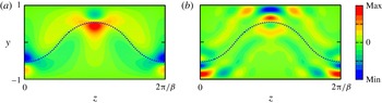
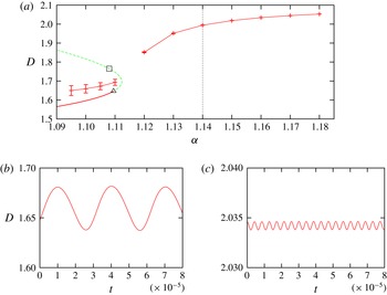
First we compute an equilibrium solution of the VWI problem using the hybrid system; see the results close to the saddle-node point shown in figure 6. Since we use Newton’s method, unlike Hall & Sherwin (Reference Hall and Sherwin2010) and Blackburn et al. (Reference Blackburn, Hall and Sherwin2013) for example, there is no difficulty in rounding the saddle-node point. The streaky fields on the upper and lower branches for
 $\overline{\unicode[STIX]{x1D6FC}}=1$
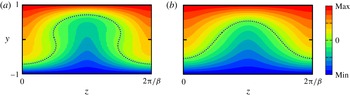
are shown in figure 7. The critical layer for the lower branch typically has a relatively flat profile, whilst the upper branch has an inflected, multi-valued critical layer.
The bifurcation diagram of the VWI equilibrium states computed by the hybrid approach for
 $\unicode[STIX]{x1D6FC}=\overline{\unicode[STIX]{x1D6FC}}$
and
 $\unicode[STIX]{x1D6FD}=1.667$
. The Rayleigh mode stability at the points indicated by arrows is examined in figure 8(b–e).

The streak field at
 $\overline{\unicode[STIX]{x1D6FC}}=1$
in figure 8(a). (a) Upper branch, (b) lower branch. The position of the critical layer is indicated by the dashed curve.

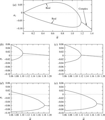
The selected Rayleigh mode growth rate
 $\unicode[STIX]{x1D70E}_{r}$
for the perturbation wavenumber
 $\widetilde{\unicode[STIX]{x1D6FC}}$
. At the vertical dotted line
 $\widetilde{\unicode[STIX]{x1D6FC}}=\overline{\unicode[STIX]{x1D6FC}}$
. The hybrid approach has been used to carry out the calculations. (a) Computed at the lower branch of figure 6 at
 $\overline{\unicode[STIX]{x1D6FC}}=1.1$
. The two real growth rates emanating on the left merge to create a pair of complex conjugate growth rates. (b–e) Computed at the points indicated by (b–e) in figure 6. Note that (d) is a close up of (a).

The most unstable non-neutral Rayleigh mode growth rate when
 $\widetilde{\unicode[STIX]{x1D6FC}}=\overline{\unicode[STIX]{x1D6FC}}$
. Note that
 $\unicode[STIX]{x1D70E}=0$
is always an eigenvalue because the wave part of the VWI interaction must be neutral. The hybrid approach has been used to produce the results.

In figure 8(a) we show the eigenvalues for a range of
 $\widetilde{\unicode[STIX]{x1D6FC}}>0$
. The result shown is computed at the point (d) in figure 6 and is typical of those found on the lower branch to the left of this point. At the origin one stable and one unstable real eigenvalue emanate and meet at a point beyond the neutral point of the unstable one. Here the eigenvalues merge into a complex conjugate pair of eigenvalues. We see that when
 $0<\widetilde{\unicode[STIX]{x1D6FC}}<\overline{\unicode[STIX]{x1D6FC}}$
there is a band of unstable disturbances. Most of the previous instability analyses using a full Navier–Stokes approach have ignored that instability. For finite Reynolds number such an unstable band can be captured by extending the computational box to accommodate several copies of the equilibrium solution in streamwise direction, or more generally by using Floquet analysis. We observed that at
 $R=20\,000$
the unstable eigenvalues computed by the former approach excellently reproduce the unstable band seen in figure 8(a). Likewise direct numerical simulations in a small box used to define edge states have not allowed for disturbances associated with this unstable band. This explains why the edge state is no longer a steady state when a large enough computational box is chosen; see Duguet, Schlatter & Henningson (Reference Duguet, Schlatter and Henningson2009), Schneider, Maric & Eckhardt (Reference Schneider, Maric and Eckhardt2010) for example.
Figure 8(b–e) shows the growth rates
 $\unicode[STIX]{x1D70E}_{r}$
near
 $\widetilde{\unicode[STIX]{x1D6FC}}=\overline{\unicode[STIX]{x1D6FC}}$
at the selected points along the solution branch. In each of the four cases we see that as
 $\widetilde{\unicode[STIX]{x1D6FC}}$
increases two real eigenvalues merge to form a complex conjugate pair of eigenvalues. For the stability results of the lower VWI branch shown in figure 8(d,e), the upper real eigenvalue passes through zero at exactly the point where
 $\widetilde{\unicode[STIX]{x1D6FC}}=\overline{\unicode[STIX]{x1D6FC}}$
. This is simply confirming that the streak is neutrally stable to the Rayleigh wave driving the VWI. The crucial result is that when the saddle-node point is rounded the point where the complex conjugate pair is born is now shifted above the horizontal axis. That result is important because it allows for the possibility of bifurcations from stationary VWI states to time periodic states.
We see that an unstable complex conjugate pair of eigenvalues comes into existence close to the point shown in figure 8(c). If we decrease
 $\overline{\unicode[STIX]{x1D6FC}}$
along the upper branch from this point, as shown in figure 8(b), the zero growth rate at
 $\widetilde{\unicode[STIX]{x1D6FC}}=\overline{\unicode[STIX]{x1D6FC}}$
is realised by the lower real eigenvalue. Therefore the upper-branch VWI state is now unstable to a Rayleigh disturbance when
 $\widetilde{\unicode[STIX]{x1D6FC}}=\overline{\unicode[STIX]{x1D6FC}}$
. Moreover, in that situation, there is an unstable pair of complex conjugate eigenvalues for shorter wavelength disturbances
 $\widetilde{\unicode[STIX]{x1D6FC}}>\overline{\unicode[STIX]{x1D6FC}}$
which then become stable at a higher value of
 $\widetilde{\unicode[STIX]{x1D6FC}}$
. This observation immediately explains why the majority of upper VWI branch cannot correspond to edge states. Figure 9 shows the hybrid stability results when
 $\widetilde{\unicode[STIX]{x1D6FC}}=\overline{\unicode[STIX]{x1D6FC}}$
. We see in the figure that the critical point where the unstable Rayleigh mode comes into existence occurs on the upper branch. It is noteworthy that the critical layer attains a multi-valued profile at
 $\overline{\unicode[STIX]{x1D6FC}}\approx 1.1$
on the upper branch, which is not so far from the point where the streak becomes Rayleigh unstable. The unstable Rayleigh mode obtained in figure 9 must be compared to that obtained from the full Navier–Stokes approach given in § 3. In figure 2 we see that with increasing
 $R$
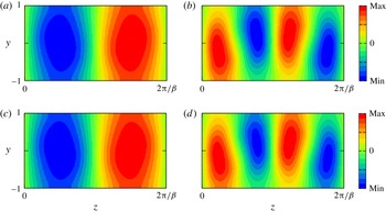
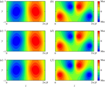
the U1 mode approaches the unstable Rayleigh mode indicated by the blue dot-dashed curve: the same result is also shown in figure 5. The corresponding pressure eigenfunctions associated with the two approaches are compared in figure 10, where we note the excellent agreement between the two results.
Comparison of the wave pressure perturbation of the unstable Rayleigh mode for
 $\unicode[STIX]{x1D6FC}=1$
at upper branch calculated from the linearised Navier–Stokes equations and using the approach of this section. (a,b) Computed using the hybrid approach, whilst (c,d) show the U1 mode in the Navier–Stokes computation for
 $R=20\,000$
; see figure 2(c,d). (a,c)
 $x=0$
, (b,d)
 $x=\unicode[STIX]{x03C0}/2\unicode[STIX]{x1D6FC}$
.

The other modes in figure 2 are apparently not Rayleigh modes since they have growth or decay rates smaller than
 $O(R^{0})$
. Note that the Rayleigh instability analysis alone does not determine the fate of the neutral eigenvalue when
 $\widetilde{\unicode[STIX]{x1D6FC}}=\overline{\unicode[STIX]{x1D6FC}}$
, which corresponds to the neutral wave sustaining the VWI equilibrium state. We recall that Wang et al. (Reference Wang, Gibson and Waleffe2007) suggested that lower-branch states had a single unstable eigenvalue which they estimated to scale like
 $R^{-0.48}$
. That eigenvalue occurs when
 $\widetilde{\unicode[STIX]{x1D6FC}}=\overline{\unicode[STIX]{x1D6FC}}$
and so would have to correspond to the neutral Rayleigh modes in figure 9. Thus the Rayleigh analysis can be interpreted as finding only the
 $O(R^{0})$
term and if that term becomes zero we might anticipate the next-order correction would give the result by Wang et al. (Reference Wang, Gibson and Waleffe2007). We will investigate this issue in § 6. The eigenvalues in figure 2 which scaled like
 $R^{-1}$
are also not connected to Rayleigh modes. Their origin is obvious since they operate on the roll–streak diffusion time scale
 $T$
, as we shall give a formal asymptotic description in the next section.
5 The slow modes occurring on the roll–streak time scale
Now let us consider the slow mode instabilities of VWI states. These modes exist on the time scale
 $T$
for roll–streak evolution and so the growth rates are
 $O(R^{-1})$
smaller than the Rayleigh modes discussed in the previous section. Whereas the Rayleigh mode calculation of the previous section is simply an inviscid stability calculation of the streak field from a VWI state, here the instability couples the roll, streak and wave parts of the flow field, and we can look at the instability within the framework of the unsteady VWI equations rather than reverting back to the full Navier–Stokes equations. The equilibrium solution of the VWI system
 $\overline{\boldsymbol{U}},\overline{P},\overline{p},\overline{c}$
for given values of the wavenumbers
 $\unicode[STIX]{x1D6FC},\unicode[STIX]{x1D6FD}$
is perturbed by writing
 $$\begin{eqnarray}\displaystyle \boldsymbol{U}=\overline{\boldsymbol{U}}+\unicode[STIX]{x1D6FF}\check{\boldsymbol{U}}\text{e}^{\check{\unicode[STIX]{x1D70E}}T},\quad P=\overline{P}+\unicode[STIX]{x1D6FF}\check{P}\text{e}^{\check{\unicode[STIX]{x1D70E}}T},\quad p=\overline{p}+\unicode[STIX]{x1D6FF}\check{p}\text{e}^{\check{\unicode[STIX]{x1D70E}}T}. & & \displaystyle\end{eqnarray}$$
The constant
 $\unicode[STIX]{x1D6FF}$
is assumed to be small enough that the VWI equations can be linearized about the equilibrium state. The equations of motion for the perturbed roll–streak flow are
 $$\begin{eqnarray}\displaystyle & \displaystyle (\check{\unicode[STIX]{x1D70E}}+\overline{\boldsymbol{U}}\boldsymbol{\cdot }\unicode[STIX]{x1D735})\check{\boldsymbol{U}}+(\check{\boldsymbol{U}}\boldsymbol{\cdot }\unicode[STIX]{x1D735})\overline{\boldsymbol{U}}=-\unicode[STIX]{x1D735}\check{P}+\unicode[STIX]{x0394}\check{\boldsymbol{U}}, & \displaystyle\end{eqnarray}$$
 $$\begin{eqnarray}\displaystyle & \displaystyle \unicode[STIX]{x1D735}\boldsymbol{\cdot }\check{\boldsymbol{U}}=0. & \displaystyle\end{eqnarray}$$
 $$\begin{eqnarray}\operatorname{div}\left({\displaystyle \frac{\unicode[STIX]{x1D735}(\check{p}E)}{[\overline{U}-\overline{c}]^{2}}}\right)-2\operatorname{div}\left({\displaystyle \frac{{\check{U}}\unicode[STIX]{x1D735}(\check{p}E)}{[\overline{U}-\overline{c}]^{3}}}\right)=0.\end{eqnarray}$$
Unlike the situation in the previous section, since we are looking only at instabilities within the framework of the VWI equations, we are now restricted to disturbances with the same downstream wavenumber as the equilibrium state. For the slow mode the critical layer position must be perturbed since the perturbed streak has the same size in
 $R$
as
 $\overline{U}$
. The perturbed critical layer position and streak are related by
 $$\begin{eqnarray}f=\overline{f}+\unicode[STIX]{x1D6FF}\check{f}\text{e}^{\check{\unicode[STIX]{x1D70E}}T},\quad \check{f}=\left.-{\displaystyle \frac{{\check{U}}}{\unicode[STIX]{x2202}_{y}\overline{U}}}\right|_{y=\overline{f}},\end{eqnarray}$$
where
 $U=\overline{c}$
at
 $y=f$
,
 $\overline{U}=\overline{c}$
at
 $y=\overline{f}$
. If we denote the component of the perturbed roll velocity field
 $(\check{V},\check{W})$
resolved in the
 $s$
direction by
 $\check{V}^{s}$
then it can be shown that the following jumps are to be applied across the critical layer;
 $$\begin{eqnarray}\left[{\displaystyle \frac{\unicode[STIX]{x2202}\check{V}^{s}}{\unicode[STIX]{x2202}n}}+\check{f}\unicode[STIX]{x2202}_{y}{\displaystyle \frac{\unicode[STIX]{x2202}\overline{V}^{s}}{\unicode[STIX]{x2202}n}}\right]_{-}^{+}=n_{0}\unicode[STIX]{x1D6FC}^{-5/3}{\displaystyle \frac{\text{d}\check{Q}}{\text{d}s}},\quad \left[\check{P}+\check{f}\unicode[STIX]{x2202}_{y}\overline{P}\right]_{-}^{+}=-n_{0}\unicode[STIX]{x1D6FC}^{-5/3}(\check{\unicode[STIX]{x1D712}}\overline{Q}+\overline{\unicode[STIX]{x1D712}}\check{Q}),\end{eqnarray}$$
where the terms on the right-hand side, which must be evaluated at
 $y=\overline{f}$
, can be calculated using
 $$\begin{eqnarray}\check{Q}=-{\displaystyle \frac{5\check{\unicode[STIX]{x1D706}}_{1}}{3\overline{\unicode[STIX]{x1D706}}_{1}}}\overline{Q}+\overline{\unicode[STIX]{x1D706}}_{1}\left({\displaystyle \frac{\unicode[STIX]{x2202}\overline{p}_{0}}{\unicode[STIX]{x2202}s}}{\displaystyle \frac{\unicode[STIX]{x2202}\check{p}_{0}^{\ast }}{\unicode[STIX]{x2202}s}}+\text{C.C.}\right),\quad \check{\unicode[STIX]{x1D712}}=\left({\displaystyle \frac{\check{f}_{zz}}{\overline{f}_{zz}}}-{\displaystyle \frac{3\tilde{f}_{z}}{2(1+\overline{f}_{z})}}\right)\overline{\unicode[STIX]{x1D712}}.\end{eqnarray}$$
Here the terms with overline/check are the corresponding equilibrium/perturbation quantities, and
 $\ast$
denotes complex conjugate. For a given VWI equilibrium state (5.2)–(5.6) constitutes an eigenvalue problem for the slow mode complex growth rate
 $\check{\unicode[STIX]{x1D70E}}.$
The solution of this problem is non-trivial since it is a partial differential equation eigenvalue problem to be solved subject to jump conditions across the perturbed interface.
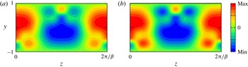
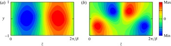
A comparison of the streak perturbation for the stable slow mode L2 for
 $\unicode[STIX]{x1D6FC}=1$
calculated from the linearised Navier–Stokes approach and the slow hybrid approach discussed in this section. (a) Hybrid slow mode computation, (b) Navier–Stokes result for
 $R=20\,000$
.

The presence of the critical layer necessitates the regularisation of the computational problem in order to find
 $\check{\unicode[STIX]{x1D70E}}$
, and so here we make use of the hybrid stability equations (3.3) to produce values of the growth rate coincident at leading order in
 $R$
with the slow mode growth rate. In order to do so, we must adjust the hybrid stability problem as we indicate below.
Firstly, the unsteady term in (3.3c
) is set equal to zero since the small growth rate on the slow time is not big enough to enter the wave problem (5.3). Then we set
 $\check{\unicode[STIX]{x1D70E}}=R\unicode[STIX]{x1D70E}\sim O(1)$
to obtain the slow eigenvalue. With this modification the hybrid equations no longer have sufficient structure to support both the Rayleigh modes and the edge modes to be described in § 6. Note however that the fictitious Reynolds number of the hybrid problem must be sufficiently large for
 $\check{\unicode[STIX]{x1D70E}}$
to be independent of
 $R_{f}$
.
The solid red lines in figure 5 are the results for the growth rate of the slow mode found by modifying the hybrid stability calculation as indicated above. We observe that there is excellent agreement between the hybrid results and the full linearised Navier–Stokes results for the stable real growth rate associated with L2. The corresponding perturbed streaks are compared in figure 11 and are also seen to be in excellent agreement. For the upper branch we believe that the complex stable growth rate mode U3 is also a slow mode. Here the evidence is not as convincing, but we believe the fact that the growth rate apparently decays slightly faster than
 $R^{-1}$
is due to our inability to calculate at sufficiently high values of
 $R$
. Note that as the Reynolds number increases the full and hybrid approaches become increasingly difficult to resolve because the critical layer at the heart of the VWI interaction shrinks.
6 The edge mode of instability
So far we have discussed two types of instability of VWI states. The first type is a Rayleigh instability of the streak part of a VWI state. Since the streak has no streamwise dependence, it is straightforward to describe perturbations with arbitrary streamwise wavenumbers. However when the streamwise wavenumber of that disturbance coincides with that of the VWI state, at least one of the possible growth rates must necessarily approach zero because the VWI state is neutral for at least one wave-like disturbance of this wavelength. On the other hand, the slow mode we considered in § 5 is associated with rather slow, gentle meanderings of the combined roll–streak–wave field. Therefore our attention in that section was restricted to a perturbation streamwise wavenumber identical to that of the unperturbed state. These modes have small
 $O(R^{-1})$
growth rates and so, at first glance, it would be reasonable to assume that the Rayleigh mode approaching neutrality as its streamwise wavenumber approaches that of the unperturbed state simply joins the spectrum of the slow modes. However we note that for the slow mode the critical layer position is deformed by the perturbation, whilst the Rayleigh mode depends only on the streak and the critical layer is not perturbed at leading order. Moreover, unlike the slow mode, the Rayleigh mode instability problem occurs on a time scale fast enough for the growth rate to enter the generalised Rayleigh equation.
We will see below that when the Rayleigh mode approaches neutrality at the VWI wavenumber it adopts a new structure having both properties of the Rayleigh and slow modes. Not surprisingly the mode lives on a time scale between the Rayleigh and slow extremes; since this mode is intrinsically linked to the edge state properties of lower-branch states we refer to it as the edge mode. The identification of the time scale on which this new mode operates requires some detailed discussion.
Suppose that we have an equilibrium solution
 $(\overline{U},\overline{V},\overline{W}),\overline{P}$
and
 $\overline{p}$
of the VWI problem; we perturb the roll–streak flow and the wave part of the VWI state by writing
 $$\begin{eqnarray}\displaystyle & \displaystyle \boldsymbol{U}=\overline{\boldsymbol{U}}+\unicode[STIX]{x1D6FF}\widetilde{\boldsymbol{U}}(y,z)\text{e}^{\check{\unicode[STIX]{x1D70E}}T}+\cdots , & \displaystyle\end{eqnarray}$$
 $$\begin{eqnarray}\displaystyle & \displaystyle P=\overline{P}+\unicode[STIX]{x1D6FF}\widetilde{P}(y,z)\text{e}^{\check{\unicode[STIX]{x1D70E}}T}+\cdots , & \displaystyle\end{eqnarray}$$
 $$\begin{eqnarray}\displaystyle & \displaystyle p=\overline{p}+\unicode[STIX]{x1D6FF}[\overline{p}+\widetilde{p}(y,z)]\text{e}^{\check{\unicode[STIX]{x1D70E}}T}+\cdots , & \displaystyle\end{eqnarray}$$
 $\widetilde{p}\ll \overline{p}$
and
 $\unicode[STIX]{x1D6FF}$
is the arbitrarily small disturbance size. We are also assuming that higher-order terms in the VWI solution do not alter the leading-order stability problem; we shall explain why this is the case later but for the clarity of our exposition we omit them. We anticipate that the modes operate on a faster time scale than does the slow mode so that the growth rate
 $\check{\unicode[STIX]{x1D70E}}$
will be large. Note here that the wave pressure perturbation at leading order has been assumed to be a simple displacement of its equilibrium form. The disturbance to the VWI state has in effect been normalized by taking the leading-order wave pressure perturbation to be of size
 $\unicode[STIX]{x1D6FF},$
and the quantities
 $\widetilde{\boldsymbol{U}},\widetilde{P},\widetilde{p}$
will have relative sizes depending on
 $\check{\unicode[STIX]{x1D70E}}$
and
 $R.$
The size of the growth rate
 $\check{\unicode[STIX]{x1D70E}}$
in
 $R$
will be derived below. The perturbed equations for the roll–streak field are:
 $$\begin{eqnarray}\displaystyle & \displaystyle (\check{\unicode[STIX]{x1D70E}}+\overline{\boldsymbol{U}}\boldsymbol{\cdot }\unicode[STIX]{x1D735})\widetilde{\boldsymbol{U}}~+(\widetilde{\boldsymbol{U}}\boldsymbol{\cdot }\unicode[STIX]{x1D735})\overline{\boldsymbol{U}}=-\unicode[STIX]{x1D735}\widetilde{P}+\unicode[STIX]{x0394}\widetilde{\boldsymbol{U}}, & \displaystyle\end{eqnarray}$$
 $$\begin{eqnarray}\displaystyle & \displaystyle \unicode[STIX]{x1D735}\boldsymbol{\cdot }\widetilde{\boldsymbol{U}}=0. & \displaystyle\end{eqnarray}$$
 $\check{\unicode[STIX]{x1D70E}}$
. The solution will therefore be inviscid away from any boundaries and the critical layer, where viscous diffusion enters in order to regularise the inviscid equations for the wave.
The stress jumps across the critical layer are perturbed by the wave and take the form
 $$\begin{eqnarray}J=\overline{J}[1+(\unicode[STIX]{x1D6FF}\text{e}^{\check{\unicode[STIX]{x1D70E}}T}+\text{C.C.})]+\cdots ,\quad K=\overline{K}[1+(\unicode[STIX]{x1D6FF}\text{e}^{\check{\unicode[STIX]{x1D70E}}T}+\text{C.C.})]+\cdots ,\end{eqnarray}$$
where
 $\overline{J}$
and
 $\overline{K}$
are the jumps defined for the equilibrium VWI; see (2.12). The perturbation stress jumps are of size
 $\unicode[STIX]{x1D6FF}$
. These jumps must be accommodated by viscous effects. We can see from the perturbed roll–streak equations above that viscous effects enter the roll–streak problem in a layer of thickness
 $O(\check{\unicode[STIX]{x1D70E}}^{-1/2})$
surrounding the critical layer. The layer has similarities with the corresponding layer in unsteady critical layer flows; see for example (Wu Reference Wu1995). Hence we use the same terminology here and henceforth we refer to it as the diffusion layer. At this stage,
 $\check{\unicode[STIX]{x1D70E}},$
which fixes the time scale over which the roll–streak field and wave pressure perturbations communicate, remains to be established. The pressure perturbation
 $\widetilde{p}$
satisfies
 $$\begin{eqnarray}\operatorname{div}\left({\displaystyle \frac{\unicode[STIX]{x1D735}(\widetilde{p}E)}{[\overline{U}-\overline{c}]^{2}}}\right)=2E\left\{{\displaystyle \frac{\unicode[STIX]{x1D735}\left[{\displaystyle \frac{\widetilde{U}}{\overline{U}-\overline{c}}}\right]\boldsymbol{\cdot }\unicode[STIX]{x1D735}\overline{p}}{[\overline{U}-\overline{c}]^{2}}}+{\displaystyle \frac{\text{i}\check{\unicode[STIX]{x1D70E}}}{\unicode[STIX]{x1D6FC}R}}{\displaystyle \frac{\unicode[STIX]{x1D735}\overline{U}\boldsymbol{\cdot }\unicode[STIX]{x1D735}\overline{p}}{[\overline{U}-\overline{c}]^{4}}}\right\}=E\left\{H_{1}+{\displaystyle \frac{\check{\unicode[STIX]{x1D70E}}}{R}}H_{2}\right\}.\end{eqnarray}$$
If
 $R^{-1}\check{\unicode[STIX]{x1D70E}}$
is
 $O(1)$
in Reynolds number then the wave perturbation would have the Rayleigh mode structure but here this is not the case since we are concerned with the time scale between the Rayleigh and slow modes. The perturbed roll–streak equations, jump conditions and wave pressure equation, i.e. (6.2)–(6.4), together with periodicity in the spanwise direction and rigid wall conditions, constitute an eigenvalue problem for
 $\check{\unicode[STIX]{x1D70E}}=\check{\unicode[STIX]{x1D70E}}(\unicode[STIX]{x1D6FC},\unicode[STIX]{x1D6FD},R).$
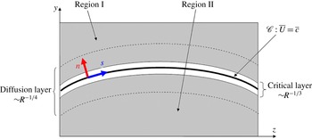
The different asymptotic regions for the edge mode.

The first step in deriving that eigenrelation is to note that since the homogeneous form of (6.4) has a solution then the inhomogeneous form will only have a solution if a solvability condition holds. In order to derive that condition we first observe that, since the operator on the left-hand side of the equation for
 $\widetilde{p}$
is self-adjoint, then if we multiply (6.4) by
 $\overline{p}$
and integrate over the regions
 $I,II$
indicated in figure 12, and add, we deduce that
 $$\begin{eqnarray}\left[\int _{\mathscr{C}}{\displaystyle \frac{\left\{\overline{p}{\displaystyle \frac{\unicode[STIX]{x2202}\widetilde{p}}{\unicode[STIX]{x2202}n}}-\widetilde{p}{\displaystyle \frac{\unicode[STIX]{x2202}\overline{p}}{\unicode[STIX]{x2202}n}}\right\}}{[\overline{U}-\overline{c}]^{2}}}\,\text{d}s\right]_{+}^{-}=\,\unicode[STIX]{x2A0D}_{I+II}\overline{p}\left\{H_{1}+{\displaystyle \frac{\check{\unicode[STIX]{x1D70E}}}{R}}H_{2}\right\}\text{d}y\,\text{d}z.\end{eqnarray}$$
Here the
 $+/-$
denote the line integral taken just above/below the critical layer and
 $n$
is measured positive above the unperturbed critical layer. The terms in (6.5) are singular as the critical layer is approached. Thus only the finite part of the integral is to be taken, because the singular behaviour must be accounted for by the terms associated with the viscous critical layer solution, as usual for this kind of analysis. Note further that we are assuming that the displacement of the critical layer can be ignored; this will be verified later. The right-hand side of (6.5) can be evaluated if
 $\widetilde{U}$
is known. We first observe that we need only to find the contribution of
 $H_{1}$
to (6.5) within the diffusion layer since the function
 $H_{2}$
has no diffusion layer structure. We will see in what follows that the dominant contribution from
 $\widetilde{U}$
to the right-hand side of (6.5) arises in the diffusion layer and that it can be evaluated explicitly so that the scaling for
 $\check{\unicode[STIX]{x1D70E}}$
deduced. The function
 $\widetilde{U}$
depends on the leading-order wave pressure perturbation through the jump conditions. We are of course implicitly assuming above that the diffusion layer is thicker than the critical layer but small compared to the channel depth; that assumption will be shown to be valid.
Next we examine the induced roll–streak flow of the perturbation in the diffusion layer. The perturbed streak is proportional to
 $\text{e}^{\check{\unicode[STIX]{x1D70E}}T}$
and, once again using body-fitted coordinates
 $(n,s)$
based on the critical layer position, the balance between normal diffusion and the time derivative in the perturbed roll–streak equations requires that
 $\unicode[STIX]{x2202}/\unicode[STIX]{x2202}n\backsimeq O(\check{\unicode[STIX]{x1D70E}}^{1/2})$
. This means that we need a diffusion layer of thickness
 $O(\check{\unicode[STIX]{x1D70E}}^{-1/2})$
straddling the critical layer. The perturbed roll–streak flow
 $\widetilde{U},\widetilde{V},\widetilde{W},\widetilde{P},$
with respect to Cartesian coordinates is replaced by
 $\widetilde{\mathscr{U}},\widetilde{\mathscr{V}},\widetilde{\mathscr{W}},\widetilde{\mathscr{P}}$
in the
 $(x,n,s)$
body-fitted coordinate system. The jump conditions suggest that the roll pressure should be
 $O(1)$
whilst the velocity field tangential to the critical layer should be
 $O(\check{\unicode[STIX]{x1D70E}}^{-1/2})$
. Continuity then suggests that the normal velocity component should be
 $O(\check{\unicode[STIX]{x1D70E}}^{-1}).$
From the perturbed streak equation we then deduce that, in the diffusion layer, the perturbed streak size is of
 $O(\check{\unicode[STIX]{x1D70E}}^{-2}).$
Thus we define a boundary layer variable
 $\unicode[STIX]{x1D702}=\check{\unicode[STIX]{x1D70E}}^{1/2}n$
and expand the perturbed roll–streak flow in the diffusion layer as
 $$\begin{eqnarray}(\widetilde{\mathscr{U}},\widetilde{\mathscr{V}},\widetilde{\mathscr{W}})=\left({\displaystyle \frac{\widetilde{\mathscr{U}}_{0}}{\check{\unicode[STIX]{x1D70E}}^{2}}},{\displaystyle \frac{\widetilde{\mathscr{V}}_{0}}{\check{\unicode[STIX]{x1D70E}}}},{\displaystyle \frac{\widetilde{\mathscr{W}}_{0}}{\check{\unicode[STIX]{x1D70E}}^{1/2}}}\right)+\cdots ,\quad \widetilde{\mathscr{P}}=\widetilde{\mathscr{P}}_{0}+\cdots ,\end{eqnarray}$$
where
 $\widetilde{\mathscr{U}}_{0},\widetilde{\mathscr{V}}_{0},\widetilde{\mathscr{W}}_{0}$
and
 $\widetilde{\mathscr{P}}_{0}$
are functions of
 $\unicode[STIX]{x1D702}$
and
 $s$
and the unperturbed quantities are to be replaced by their Taylor series expansions in
 $n$
. The equations to determine the leading-order terms in these expansions are found to be
 $$\begin{eqnarray}\displaystyle \left.\begin{array}{@{}c@{}}\widetilde{\mathscr{U}}_{0\unicode[STIX]{x1D702}\unicode[STIX]{x1D702}}-\widetilde{\mathscr{U}}_{0}=\widetilde{\mathscr{V}}_{0}\unicode[STIX]{x1D706}_{1}+\widetilde{\mathscr{W}}_{0}\unicode[STIX]{x1D706}_{1}^{\prime }\unicode[STIX]{x1D702},\quad \widetilde{\mathscr{P}}_{0\unicode[STIX]{x1D702}}=0,\\ \widetilde{\mathscr{W}}_{0\unicode[STIX]{x1D702}\unicode[STIX]{x1D702}}-\widetilde{\mathscr{W}}_{0}=0,\quad \widetilde{\mathscr{W}}_{0s}+\widetilde{\mathscr{V}}_{0\unicode[STIX]{x1D702}}=0,\end{array}\right\} & & \displaystyle\end{eqnarray}$$
subjected to the jump conditions across the critical layer
 $$\begin{eqnarray}\displaystyle \left.\begin{array}{@{}c@{}}[\widetilde{\mathscr{U}}_{0}]_{-}^{+}=[\widetilde{\mathscr{U}}_{0\unicode[STIX]{x1D702}}]_{-}^{+}=[\widetilde{\mathscr{V}}_{0}]_{-}^{+}=[\widetilde{\mathscr{W}}_{0}]_{-}^{+}=0,\\ \text{}[\widetilde{\mathscr{W}}_{0\unicode[STIX]{x1D702}}]_{-}^{+}=\overline{J},\quad [\widetilde{\mathscr{P}}_{0}]_{-}^{+}=\overline{K}.\end{array}\right\} & & \displaystyle\end{eqnarray}$$
The above system is readily solved and, denoting the solutions above and below the critical layer by
 $\pm ,$
yields for the roll flow
 $$\begin{eqnarray}\widetilde{\mathscr{W}}_{0}^{\pm }=-{\displaystyle \frac{\overline{J}\text{e}^{\mp \unicode[STIX]{x1D702}}}{2}},\quad \widetilde{\mathscr{V}}_{0}^{\pm }=\mp {\displaystyle \frac{\overline{J}^{\prime }}{2}}[\text{e}^{\mp \unicode[STIX]{x1D702}}-1]+B,\quad \widetilde{\mathscr{P}}_{0}=C\pm {\displaystyle \frac{\overline{K}}{2}},\end{eqnarray}$$
whilst the streak is given by
 $$\begin{eqnarray}\widetilde{\mathscr{U}}_{0}^{\pm }=\pm {\displaystyle \frac{\unicode[STIX]{x1D706}_{1}^{\prime }\overline{J}}{8}}\unicode[STIX]{x1D702}^{2}\text{e}^{\mp \unicode[STIX]{x1D702}}+{\displaystyle \frac{[2\unicode[STIX]{x1D706}_{1}\overline{J}^{\prime }+\unicode[STIX]{x1D706}_{1}^{\prime }\overline{J}]}{8}}\unicode[STIX]{x1D702}\text{e}^{\mp \unicode[STIX]{x1D702}}\pm {\displaystyle \frac{\unicode[STIX]{x1D706}_{1}\overline{J}^{\prime }}{2}}[\text{e}^{\mp \unicode[STIX]{x1D702}}-1]-\unicode[STIX]{x1D706}_{1}B.\end{eqnarray}$$
Here
 $B(s),C(s)$
are as yet arbitrary functions of distance along the critical layer. We note that
 $\widetilde{\mathscr{U}}_{0}^{\pm }$
tend to constants at the edge of the diffusion layer so that the perturbed streak persists throughout the channel. The roll component along the critical layer decays to zero outside the diffusion layer whilst the normal velocity component tends to a function of
 $s$
. It is important to notice that if
 $\check{\unicode[STIX]{x1D70E}}$
is real and negative then the roll flow can no longer be forced to decay exponentially. In that case higher-order terms in the expansion of
 $\check{\unicode[STIX]{x1D70E}}$
must be retained in order to allow the roll to decay in an outer region surrounding the diffusion layer. As we shall see at the end of this section our calculations suggest that the scenario just discussed is possible and indeed the results are consistent with the suggested scalings.
Away from the diffusion layer the flow is dominated by inviscid effects and, reverting to Cartesian coordinates and using the above properties of the perturbed roll and streak at the edge of the diffusion layer, we arrive at the expansions
 $$\begin{eqnarray}\widetilde{\boldsymbol{U}}=\left({\displaystyle \frac{\widetilde{U}_{0}}{\check{\unicode[STIX]{x1D70E}}^{2}~}},{\displaystyle \frac{\widetilde{V}_{0}}{\check{\unicode[STIX]{x1D70E}}}},{\displaystyle \frac{\widetilde{W}_{0}}{\check{\unicode[STIX]{x1D70E}}}}\right)+\cdots ,\quad \widetilde{P}=\widetilde{P}_{0}+\cdots .\end{eqnarray}$$
At leading order we see that the roll flow satisfies the potential flow equations with prescribed tangential and normal stress jumps across the critical layer. More precisely we find that the leading-order roll problem becomes
 $$\begin{eqnarray}\displaystyle \unicode[STIX]{x0394}\widetilde{P}_{0}=0,\quad [\widetilde{P}_{0}]_{-}^{+}=\overline{K},\quad [\boldsymbol{n}\boldsymbol{\cdot }\unicode[STIX]{x1D735}\widetilde{P}_{0}]_{-}^{+}=-\overline{J}, & & \displaystyle\end{eqnarray}$$
where
 $\widetilde{P}_{0y}$
should vanish on the walls. Given
 $\widetilde{P}_{0}$
the leading-order approximation to the roll–streak flow away from the diffusion layer is then given by
 $(\widetilde{U}_{0},\widetilde{V}_{0},\widetilde{W}_{0})=(\widetilde{P}_{0y}\overline{U}_{y}+\widetilde{P}_{0z}\overline{U}_{z},-\widetilde{P}_{0y},-\widetilde{P}_{0z})$
, and thus the functions
 $B(s)$
and
 $C(s)$
are then given by
 $B(s)=\boldsymbol{n}\boldsymbol{\cdot }(\widetilde{V}_{0},\widetilde{W}_{0})+\overline{J}^{\prime }/2$
and
 $C(s)=\widetilde{P}_{0}$
 $-\overline{K}/2$
evaluated above the critical layer. The potential flow problem (6.12) can be formally solved using Green’s functions but, since it will turn out that the eigenrelation (6.5) does not depend on it, we do not give the details here.
Now let us consider the right-hand side of (6.5). As mentioned previously
 $H_{2}$
has no structure within the diffusion layer and is of
 $O(1)$
in
 $R$
. Thus we concentrate on the evaluation of the volume integral associated with
 $H_{1}.$
Away from the diffusion layer the contribution to the integral from the region outside the diffusion layer is
 $O(\check{\unicode[STIX]{x1D70E}}^{-2})$
, whilst the contribution from within the diffusion layer is
 $O(\check{\unicode[STIX]{x1D70E}}^{-1})$
. The contribution to the integral from the diffusion layer is most easily evaluated using body-fitted coordinates and using the representation (6.10) of the streak field and expanding functions having no diffusion layer structure in Taylor series around the critical layer location. After some analysis we find that the left-hand side of (6.5) becomes
 $$\begin{eqnarray}{\displaystyle \frac{2}{\check{\unicode[STIX]{x1D70E}}}}\displaystyle \unicode[STIX]{x2A0D}_{-\infty }^{\infty }\displaystyle \int _{\mathscr{C}}\left\{{\displaystyle \frac{2\overline{p}_{0}\overline{p}_{2}}{\unicode[STIX]{x1D706}_{1}^{3}\unicode[STIX]{x1D702}}}{\displaystyle \frac{\unicode[STIX]{x2202}}{\unicode[STIX]{x2202}\unicode[STIX]{x1D702}}}\left({\displaystyle \frac{\widetilde{\mathscr{U}}_{0}}{\unicode[STIX]{x1D702}}}\right)+{\displaystyle \frac{\overline{p}_{0}\overline{p}_{0}^{\prime }}{\unicode[STIX]{x1D706}_{1}^{2}\unicode[STIX]{x1D702}^{3}}}{\displaystyle \frac{\unicode[STIX]{x2202}}{\unicode[STIX]{x2202}s}}\left({\displaystyle \frac{\widetilde{\mathscr{U}}_{0}}{\unicode[STIX]{x1D706}_{1}}}\right)\right\}\,\text{d}s\,\text{d}\unicode[STIX]{x1D702}+{\displaystyle \frac{\check{\unicode[STIX]{x1D70E}}}{R}}\displaystyle \unicode[STIX]{x2A0D}_{I+II}\overline{p}H_{2}\,\text{d}y\,\text{d}z.\end{eqnarray}$$
The first integral is of
 $O(1)$
and must be taken along the critical layer. Using the form for the perturbed streak (6.10) and (2.9) it can be simplified further. If the two terms in (6.13) are to balance, we deduce that
 $\check{\unicode[STIX]{x1D70E}}$
must be
 $O(R^{1/2})$
so that the diffusion layer is of thickness
 $O(R^{-1/4})$
, consistent with our assumption that it is thicker than the critical layer. From (6.4) outside the diffusion layer
 $\widetilde{p}$
is driven only by the term associated with
 $H_{2}$
. This means that
 $\widetilde{p}$
must be of
 $O(R^{-1/2})$
in the majority of the flow and indeed smaller than the leading-order wave pressure disturbance, as assumed.
Next we consider the line integral on the left-hand side of (6.5) where only the finite part must be taken. We first note that, in view of (6.4),
 $\widetilde{p}$
can be split into a part forced by the perturbed streak flow and another one forced by the perturbed eigenvalue. Using the series solution for the pressure perturbation near the critical layer together with the fact that
 $\widetilde{\mathscr{U}}_{0\unicode[STIX]{x1D702}\unicode[STIX]{x1D702}}$
vanishes at
 $\unicode[STIX]{x1D702}=0$
it is easy to show that the contribution to the line integral from the former part vanishes. We can also show that the contribution to the line integral from the term proportional to the perturbed eigenvalue vanishes. This part does not have a diffusion layer structure and can be further split into a term which behaves like the homogeneous solution (2.8), replacing the functions
 $(\overline{p}_{0},\overline{p}_{3})$
by different functions
 $(\widehat{p}_{0},\widehat{p}_{3})$
say, and the particular integral term that behaves like
 $$\begin{eqnarray}\displaystyle q_{1}(s)n+q_{2L}(s)n^{2}\ln |n|+q_{2}(s)n^{2}+q_{3LL}n^{3}\ln |n|+q_{3L}(s)n^{3}\ln |n|+0\times n^{3}+\cdots \qquad & & \displaystyle\end{eqnarray}$$
near the critical layer. The coefficients in the above expansion do not depend on
 $(\widehat{p}_{0},\widehat{p}_{3})$
and can be fixed by the local expansion. In order to prove the vanishing of the line integral we only need the fact that the perturbed eigenvalue is so small that it does not alter the jump condition for
 $\widehat{p}_{3}$
from that for the homogeneous case (see the comments just after 2.11), and
 $q_{3L}$
does not jump across the critical layer. Therefore, the left-hand side of (6.5) vanishes identically.
Applying the rescaling
 $\check{\unicode[STIX]{x1D70E}}=R^{1/2}\widehat{\unicode[STIX]{x1D70E}}$
to (6.13), and after some manipulation, we deduce the eigenrelation of the edge mode as
 $$\begin{eqnarray}\displaystyle \widehat{\unicode[STIX]{x1D70E}}^{2}={\displaystyle \frac{\displaystyle \int _{\mathscr{C}}{\displaystyle \frac{(\overline{p}_{0}^{\prime 2}+\unicode[STIX]{x1D6FC}^{2}\overline{p}_{0}^{2})}{2\unicode[STIX]{x1D706}_{1}}}\left({\displaystyle \frac{\overline{J}}{\unicode[STIX]{x1D706}_{1}}}\right)^{\prime }\,\text{d}s}{\displaystyle \unicode[STIX]{x2A0D}_{I+II}\overline{p}H_{2}\,\text{d}y\,\text{d}z}}\equiv \unicode[STIX]{x1D6F7}. & & \displaystyle\end{eqnarray}$$
When the symmetry (2.14) is assumed,
 $\unicode[STIX]{x1D6F7}$
is a real constant, and if that constant is positive, there must be an unstable and a stable eigenvalue.
We note that the size of the perturbed streak is of
 $O(R^{-1})$
so that the critical layer position will be changed by a similar amount. It is straightforward to show that this means that the perturbed jump conditions we used, (6.3), are correct at leading order. We also commented earlier that we were performing a stability analysis of the VWI state ignoring higher-order terms in its asymptotic expansion. Even if such terms are included the edge mode stability result (6.15) is unchanged to leading order. For example in the VWI approach the viscous wall layers of the wave do not play a role in the leading-order problem.
Whilst the asymptotic analysis shows the emergence of a diffusion layer surrounding the critical layer and gives a formal expression, (6.15), for the eigenrelation, the numerical evaluation of the integrals in (6.15) is still challenging. The major difficulty is due to the extremely difficult numerical evaluation of the principal value integrals associated with
 $H_{2}$
. Firstly,
 $\overline{p}_{0},\overline{p}_{2},\overline{p}_{3L},\unicode[STIX]{x1D706}_{1}$
and various derivatives along the critical layer of these functions derivatives have to be extracted from the VWI equilibrium state; that task alone is difficult once the critical layer is significantly deformed from the horizontal and that is the case for the equilibrium states considered here. Moreover, having done that extraction, the principal value integrals need to be evaluated by subtracting out singularities as severe as
 $\unicode[STIX]{x1D702}^{-4}$
. Those tasks proved impossible for us to achieve with any reasonable accuracy within the constraints of our computational scheme. Therefore, as in § 5, rather than calculating the eigenvalues directly, we simply relate the computational problem to one which produces the leading-order growth rate through an indirect approach using the hybrid system.
Obviously we cannot neglect the unsteady term in the wave equation (3.3c ) as we did for the slow mode hybrid problem and thus the reduction must be modified. In order to preclude the possibility of the slow mode, the reduction of the roll–streak part is indeed possible noting that the equilibrium roll component does not play any role in the above asymptotic theory. In fact, the reduced form of (6.2)
 $$\begin{eqnarray}\displaystyle & \displaystyle \check{\unicode[STIX]{x1D70E}}\left[\begin{array}{@{}c@{}}\widetilde{U}\\ \widetilde{V}\\ \widetilde{W}\end{array}\right]+\left[\begin{array}{@{}c@{}}(\widetilde{V}\unicode[STIX]{x2202}_{y}+\widetilde{W}\unicode[STIX]{x2202}_{z})\overline{U}\\ \unicode[STIX]{x2202}_{y}\widetilde{P}\\ \unicode[STIX]{x2202}_{z}\widetilde{P}\end{array}\right]=\unicode[STIX]{x1D6E5}\left[\begin{array}{@{}c@{}}\widetilde{U}\\ \widetilde{V}\\ \widetilde{W}\end{array}\right], & \displaystyle\end{eqnarray}$$
 $$\begin{eqnarray}\displaystyle & \displaystyle \unicode[STIX]{x2202}_{y}\widetilde{V}+\unicode[STIX]{x2202}_{z}\widetilde{W}=0, & \displaystyle\end{eqnarray}$$
 $\unicode[STIX]{x1D70E}$
by
 $R^{-1/2}\widehat{\unicode[STIX]{x1D70E}}$
.
The results of the hybrid asymptotic computation for the edge mode growth rates are represented in figure 5 by solid lines. On the upper branch there is a single unstable edge mode predicted by the asymptotic hybrid approach and in figure 5(a) we see that it agrees excellently with the results from the Navier–Stokes calculations. Likewise we see in figure 5(c) that on the lower branch the asymptotic hybrid approach gives excellent agreement with the Navier–Stokes predictions of
 $\unicode[STIX]{x1D70E}_{r}$
for both L1 and L3. These growth rates have similar magnitude and thus may correspond to the pair of leading-order eigenvalues predicted by (6.15). The asymptotic hybrid approach is not however sensitive enough to pick out the asymptotically smaller imaginary part of the frequency. In figure 5(d) we have drawn a dotted line of slope
 $-5/8$
which suggests that a higher-order asymptotic theory would produce frequencies of the complex conjugate edge modes of size
 $R^{-5/8}$
.
In order to deduce the scaling for the frequency of L3 we first write (6.15) in the unscaled form
 $$\begin{eqnarray}{\displaystyle \frac{\check{\unicode[STIX]{x1D70E}}}{R}}={\displaystyle \frac{\unicode[STIX]{x1D6F7}}{\check{\unicode[STIX]{x1D70E}}}},\end{eqnarray}$$
but we now allow for higher-order corrections to the leading-order growth rate. Note that in our discussion of the edge mode we effectively took the branch of
 $\check{\unicode[STIX]{x1D70E}}^{1/2}$
with positive real part so for our discussion leading to the above equation to be valid we need either
 $\check{\unicode[STIX]{x1D70E}}$
to be positive at leading order or, for the stable case, a higher-order term in the expansion of
 $\check{\unicode[STIX]{x1D70E}}$
must have non-zero imaginary part. The next-order correction to the growth rate is found by bringing in the next-order contribution from the diffusion layer. If the higher-order correction term has non-zero imaginary part then our discussion in § 6 concerning the diffusion layer remains formally valid since the higher-order terms push the eigenvalue away from the negative real axis. This means that (6.15) is in fact valid for both the unstable and stable modes and that the growth rate of the unstable mode is simply the negative of that of the stable one at leading order. That result is consistent with our numerical calculations of the full problem; see for example figure 2. The next-order term is of relative order the same as the thickness of the layer. For the unstable case the layer is of thickness
 $\check{\unicode[STIX]{x1D70E}}^{-1/2}$
and so if we write
 $$\begin{eqnarray}\check{\unicode[STIX]{x1D70E}}=\unicode[STIX]{x1D6F7}^{1/2}R^{1/2}+\check{\unicode[STIX]{x1D70E}}_{1},\end{eqnarray}$$
then the size of the correction term is fixed as follows. Firstly, the next-order correction to the diffusion layer solution produces a term on the left-hand side
 ${\sim}R^{-1}\unicode[STIX]{x1D6F7}^{1/2}R^{1/2}\check{\unicode[STIX]{x1D70E}}^{-1/2}.$
On the other hand, since the growth rate is perturbed, there will also be a term proportional to
 $R^{-1}\check{\unicode[STIX]{x1D70E}}_{1}.$
If we require these effects to balance then we arrive at the scaling
 $$\begin{eqnarray}\check{\unicode[STIX]{x1D70E}}_{1}\sim R^{1/4}.\end{eqnarray}$$
Thus as we might have anticipated the correction to the growth rate is of relative size equal to the diffusion layer thickness. For the stable mode though a subtle difference now arises because
 $\check{\unicode[STIX]{x1D70E}}^{1/2}$
is purely imaginary at leading order. Therefore the diffusion layer is now of relative thickness
 $[\unicode[STIX]{x1D6F7}^{1/2}R^{1/2}]^{1/2}/\check{\unicode[STIX]{x1D70E}}_{1}.$
In this case the requirement that the corrections to the left-hand side of the above unscaled form for the growth rate due to perturbing the growth rate and higher-order diffusion layer effects should balance is
 $$\begin{eqnarray}{\displaystyle \frac{1}{R^{1/2}}}{\displaystyle \frac{[\unicode[STIX]{x1D6F7}^{1/2}R^{1/2}]^{1/2}}{\check{\unicode[STIX]{x1D70E}}_{1}}}\sim {\displaystyle \frac{\check{\unicode[STIX]{x1D70E}}_{1}}{R}}\end{eqnarray}$$
so that in the stable case we deduce that
 $\check{\unicode[STIX]{x1D70E}}_{1}\sim \pm \text{i}R^{3/8}.$
In that case, the diffusion layer is of thickness
 $R^{-1/8}$
. Note also that the above balance leads to a complex conjugate pair of eigenvalues. If the frequency behave like
 $R^{3/8}$
on the time scale
 $T$
, it behaves like
 $R^{-5/8}$
on the time scale
 $t$
and this explains why we choose to draw a line of slope
 $-5/8$
in figure 5(c,d). We conclude then that the next-order correction to the unstable mode is of relative order
 $R^{-1/4}$
whilst the stable branch L3 has purely imaginary correction terms appearing of relative order
 $R^{-1/8}.$
That conclusion is in perfect agreement with our numerical calculations of the full stability problem.
Now let us turn to a comparison of the eigenfunctions predicted by our asymptotic description of the edge mode and the Navier–Stokes calculations. The key property of the edge mode is that the perturbed wave pressure is at leading-order proportional to the undisturbed wave pressure of the VWI state. Figure 13(a–d) shows the pressure eigenfunction of L1 mode associated with the hybrid stability computation and Navier–Stokes stability computation for
 $R=20\,000$
respectively. Consistent with the expansion of the pressure (6.1c
), we can see both of the pressure fields are dominated by the equilibrium pressure shown in figure 13(e,f). Figure 14 shows the Navier–Stokes computation of the wave pressure field for the stable complex mode L3 and it is again consistent with the equilibrium wave pressure.
Next we consider the asymptotic prediction of the perturbed streak with the Navier–Stokes calculation of that quantity; see figure 15. In that figure we see that the mode L1 has a diffusion layer structure surrounding the critical layer before relaxing to a structure varying on an
 $O(1)$
scale elsewhere. That result is certainly consistent with our asymptotic prediction. The corresponding figure for the complex stable mode L3 shows a slight modification of that structure with the diffusion layer now thickening and signs of a cellular structure developing in the direction normal to the critical layer, entirely consistent with the asymptotic structure for the stable edge mode we described above.
Comparison of the wave pressure perturbation of the edge mode labelled L1 for
 $\unicode[STIX]{x1D6FC}=1$
. (a,b) Computed by the hybrid approach, whilst (c,d) show the L1 mode in the Navier–Stokes computation for
 $R=20\,000$
; see figure 2(c,d). (a,c,e)
 $x=0$
, (b,d,f)
 $x=\unicode[STIX]{x03C0}/2\unicode[STIX]{x1D6FC}$
. In (e,f) we show the equilibrium pressure of the lower-branch state computed by the hybrid method.

The same plot as figure 13(c,d) but for the L3 mode.

The real part of streak perturbation of edge mode Navier–Stokes computation for
 $\unicode[STIX]{x1D6FC}=1$
and
 $R=20\,000$
. (a) L1 mode developing a sublayer structure. (b) L3 mode developing a oscillating sublayer structure.

7 Conclusions and discussion
We have seen that there are three possible modes of instability of VWI states which grow or decay on the roll–streak time scale, the wave time scale or one midway between the two. The derivations of the asymptotic structures of the first two modes were rather straightforward, since the time scales of these modes correspond to those of wave and roll–streak parts of the VWI equilibrium. The first mode we investigated has been effectively ignored in most of the previous Navier–Stokes investigations by restricting the streamwise wavenumber of the disturbance. The mode we discussed is essentially a Rayleigh instability of the streak part of the equilibrium state and grows on the inviscid
 $O(R^{0})$
time scale. Since the streak has no streamwise dependence, it was not necessary to restrict the stability analysis to perturbations with the streamwise wavenumber equal to its equilibrium value. The second mode we considered is a slow mode associated with a much weaker gentle meandering of the combined roll–streak–wave field of the equilibrium state and our attention was restricted to a perturbation streamwise wavenumber identical to that of the unperturbed state. The slow mode instability occurs on the roll–streak diffusion time scale of
 $O(R)$
and thus the perturbed streak alters the critical layer position by an
 $O(R^{0})$
amount in this time scale. When the imposed disturbance has the same downstream wavenumber as the equilibrium state one of the Rayleigh modes weakens into what is essentially the single unstable mode associated with edge states. The new structure appearing in this case is driven by a combined roll–streak–wave instability as was the case for the slow mode. However, the induced streak perturbation is sufficiently small that the critical layer position is unchanged to leading order. We referred to the newly identified instability having both properties of the Rayleigh and slow modes as the edge mode. It is found that the numerically predicted growth rate scaling of
 $R^{-0.48}$
in Wang et al. (Reference Wang, Gibson and Waleffe2007) corresponds to the edge mode scaling of
 $R^{-1/2}$
found here. Our theory of the edge mode in § 6 showed that there are unstable and stable edge modes. From the higher-order effect the stable edge mode becomes a pair of complex conjugate eigenvalues with the imaginary part asymptotically smaller than the real part.
Therefore VWI states are susceptible to instabilities living on time scales
 $t=O(R^{0}),O(R^{1/2})$
and
 $O(R)$
corresponding to Rayleigh, edge and slow modes, respectively. The formal asymptotic theories for these modes were given in §§ 4–6. The Navier–Stokes computations performed in § 3 for relatively large Reynolds numbers are consistent with these three scalings. Also, consistent with the numerical investigations by previous authors, we found lower-branch states to be unstable to only one edge mode instability. On the other hand, the reason why the upper branch cannot act as an edge state is that the streaky field for this case is strongly altered from the lower-branch state so that it can support unstable Rayleigh modes. In order to evaluate the asymptotic predictions of the different growth rates and produce a quantitative comparison to the asymptotic results with the Navier–Stokes computations, hybrid approaches were employed for the computation of the asymptotically reduced systems.
The hybrid framework is primarily based on the linear stability of the VWI equilibrium solved by the hybrid approach by Blackburn et al. (Reference Blackburn, Hall and Sherwin2013), and then the perturbed hybrid equations are further reduced for each of the three modes. For the Rayleigh mode only the wave part of the perturbed hybrid equations is used to compute an approximation of the inviscid instability for a given streak. In contrast the hybrid slow mode computation proceeds by neglecting the time derivative in the wave part since this mode evolves in the roll–streak time scale. To evaluate the edge mode eigenvalues both the roll–streak and wave parts of the perturbed hybrid equations must have the time derivatives retained. In the hybrid computation of the edge mode the special structure of roll–streak perturbation found by the asymptotic analysis is used to reduce the roll–streak perturbed hybrid equations.
The full Navier–Stokes calculations at sufficiently large Reynolds numbers suggest that there are several reconnections of the stability modes near the saddle node. For example, in § 3, the unstable growth rate of the Rayleigh mode type, labelled U1, must decrease and become of
 $O(R^{-1/2})$
as it approaches the point where it connects the edge modes labelled U2 and L3. Likewise the unstable eigenvalue of edge mode type labelled L1 must decrease to become
 $O(R^{-1})$
before it connects to the slow modes labelled by L2 and U3. In order to find the asymptotic structure of these reconnections the value of
 $\unicode[STIX]{x1D6FC}$
may also need to perturbed around the critical value but such analysis is beyond the scope of this paper.
The variation of the drag on the lower wall
 $D$
with
 $R=3000$
,
 $\unicode[STIX]{x1D6FD}=1.667$
. (a) The points with error bars indicate periodic solutions. The curves shown at
 $\unicode[STIX]{x1D6FC}=1.09{-}1.11$
are the steady solutions we have investigated in the previous sections. All solutions of edge states type are shown by red: these solutions only have one unstable eigenvalue. The upper steady solution branch shown by the dashed green curve has more than one unstable eigenvalue thus is not a edge state. The square and triangle correspond to the neutral points shown in figure 3. The vertical dotted line is the minimal flow unit by Hamilton et al. (Reference Hamilton, Kim and Waleffe1995). (b) Temporal oscillation of the periodic solution for
 $\unicode[STIX]{x1D6FC}=1.1$
. (c) Temporal oscillation of the periodic solution for
 $\unicode[STIX]{x1D6FC}=1.16$
.

Near the saddle node there are three neutral points as shown in figure 3. One of the neutral points associated with L2 corresponds to the obvious neutral point at the saddle node, and the other neutral points at the upper and lower branches may be responsible for bifurcations to new solution branches. The imaginary parts of the growth rates do not vanish at the latter two neutral points, so we expect the bifurcations to lead to periodic solutions. To find periodic solutions around the neutral points direct numerical simulations were performed at
 $R=3000$
assuming symmetries (2.14) and our calculations are shown in figure 16(a). Here, the amplitude of the initial conditions are carefully chosen so that the trajectory will converge to the edge of the laminar and turbulent attractors; see Itano & Toh (Reference Itano and Toh2001). The simulations detect a family of rapidly oscillating solutions at relatively large streamwise wavenumber: see figure 16(b). The amplitude of the oscillation of the solution is much smaller than the amplitude of the time-independent part and this almost steady character of the solution is similar to the edge mode.
Thus it is highly likely that the rapidly oscillating solution is associated with a bifurcation from the neutral point associated with L3 indicated by the triangle in figure 16(a). This result confirms that the bifurcation of the ‘gentle solution’ found in Kawahara & Kida (Reference Kawahara and Kida2001) from the lower branch of the steady solutions found by Nagata (Reference Nagata1990) will persist at large Reynolds numbers. On the other hand, a different type of periodic solutions with longer period is found at relatively small streamwise wavenumber: see figure 16(c). For these periodic solutions has relatively large change of its amplitude in one period similar to the behaviour we found for the slow modes so they may connect to the neutral point associated with U3 indicated by the square in figure 16(a). In Kawahara & Kida (Reference Kawahara and Kida2001) they reported another interesting class of periodic solutions which accurately approximate turbulent trajectories; those solutions again have the amplitude of the solution changing by an
 $O(1)$
amount over one period. Thus it is of interest to seek a connection of their work and the present study. In order to find the scaling and the fate of the periodic solutions near the neutral points further investigation must be done using Newton’s method but we do not pursue that here.
Finally we remark that, although our attention in this study was on plane Couette flow, the VWI framework applies to rather arbitrary flow configurations. Therefore we expect that the three stability modes of large Reynolds number equilibrium states would exist in any unidirectional shear flows. For example, the
 $R^{-0.41}$
and
 $R^{-0.87}$
scalings of the unstable growth rates of pipe flow solutions obtained by Viswanath (Reference Viswanath2009) are likely to be the edge and slow modes proposed in this study. We believe that even for developing flows such as boundary layers the scenario would be identical. In the developing flow we can introduce a slow non-parallel streamwise scale where the slow streamwise scale plays similar role as time in the temporal problem; see Hall & Smith (Reference Hall and Smith1991). Therefore the structure of the temporal stability modes derived in this paper would also be able to found in the spatial instability of coherent structures.
Acknowledgements
The authors acknowledge the support of this work by EPSRC through the grant EP/I037946/1. The authors thank the referees on the helpful comments on the paper.