FEDERAL SPENDING AND PRIOR ESTIMATES OF ITS IMPACT IN THE 1930S

In the aftermath of World War I, Republican Presidents and Congresses ran surpluses to pay down the war debt. After the 1922 Recession, real tax revenues and expenditures in Figure 1 held steady through fiscal year 1929 at roughly 30 billion and 23.5 billion 1996 dollars, respectively. Although President Hoover and the Republican Congresses actively proselytized for balanced budgets and voluntarism, they raised real federal expenditures by 88 percent between the fiscal years 1929 and 1932 within the context of existing programs. They tripled road spending and Bureau of Reclamation irrigation loans and nearly doubled the Army Corps of Engineers spending on rivers and harbors. Program reports indicate the spending was intended to stimulate the economy. For example, the U.S. Department of Agriculture (1932, pp. 49–50) described the impact of increase in highway spending in 1932 as follows: “Emergency employment was directly provided for varying periods for nearly 200,000 men and indirectly for a much larger number in industries that supply necessary materials and services.” In February 1932 the Hoover administration and Republican Congress established the Reconstruction Finance Corporation (RFC), which offered loans to support the banking system, industry, and local relief programs. Nevertheless, the same politicians are more famous for holding federal spending roughly constant in fiscal 1933, as unemployment rates soared above 20 percent. In attempts to balance the budget and increase tax revenue, they also raised income and excise tax rates. As a result, total revenues in Figure 1 held steady as receipts from the excise tax increases offset a sharp drop in income tax receipts (Fishback Reference Fishback2010).

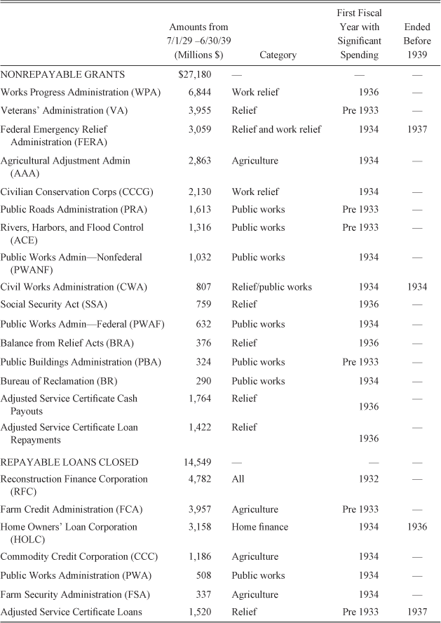
The Roosevelt administration started from this elevated level of spending and proceeded to raise real federal expenditures by 76.5 percent through 1939 (see Figure 1). The deficit in real terms remained roughly constant relative to 1932 because Democrats largely sought to honor the balanced budget pledges Roosevelt made in his 1932 election campaign. Thus, Figure 1 shows that federal revenues rose at roughly the same speed as federal spending. E. Cary Brown (Reference Brown1956) and Larry Peppers (Reference Brown1973) found that the federal deficits during this period fell well short of being Keynesian policies designed to stimulate the economy.Footnote ⁴ Even though these were not Keynesian deficits, the deficits were large enough that the expansions in spending under the Hoover and Roosevelt administration led to an increase in the federal debt as a percentage of Gross Domestic Product (GDP) from 16 percent in 1929 to 44 percent in 1939 (Fishback Reference Brown2010, p. 410). The lion's share of the new outlays came in the form of new programs, as seen by the long list of programs in Table 1 that started in fiscal year 1934, the first year when Roosevelt and the Democratic Congress had full control of the budget.

Table 1

TOTAL AND PER CAPITA FEDERAL FUNDS DISTRIBUTED TO THE STATES FOR MAJOR PROGRAM IN MILLIONS OF CONTEMPORARY DOLLARS FOR THE PERIOD 1 JULY 1932 THROUGH 30 JUNE 1939

Source:

Data compiled from OGR (1939).

The rapid rise in New Deal spending has not gone unnoticed and economic historians have tried to estimate the impact of New Deal spending on national economic activity. Christina Romer (Reference Brown1992) calculates a fiscal multiplier of only 0.23 in a difference-in-difference estimate that examined the change in federal funds distributed after the Veterans’ Bonus was passed out in 1936. Joshua Hausmann (Reference Cullen and Fishback2013) finds that the Veterans’ Bonus in 1936 (adjusted service certificate payments in Table 1) stimulated income, as well as automobile sales and building permits. In studies focused on local areas, Price Fishback, William Horrace, and Shawn Kantor (Reference Fishback, Horrace and Kantor2005, Reference Fishback, Horrace and Kantor2006) showed a strong positive influence of public works and relief spending on county-level retail sales and net-migration. Tom Garrett and David Wheelock (Reference Garrett and Wheelock2006) found similar positive effects of overall New Deal spending in a cross-sectional analysis of the growth rate in state personal income per capita for the entire period 1933 to 1939 and New Deal spending during that period. However, neither article uses annual information and thus produces no annual multiplier.

In studies of panel data for cities between 1929 and 1940, Fishback, Michael Haines, and Kantor (Reference Fishback, Haines and Kantor2007) and Ryan Johnson, Fishback, and Kantor (Reference Brown2010) show that relief spending contributed to reductions in mortality and crime rates and increases in birth rates. Studies of labor markets using panel data from 1930s have focused on the impact of relief spending on labor markets. Todd Neumann, Fishback, and Kantor (Reference Fishback2010) examine monthly data from 1933 through 1940 for more than 40 cities and find that relief spending raised private employment through 1935 but reduced it afterward. Daniel Benjamin and Kent Mathews (Reference Benjamin and Mathews1992) find small crowding out effects of private employment from relief jobs through 1935 and much larger crowding out effects in the second half of the New Deal. In cross-sectional estimation, Robert Fleck (Reference Fleck1999) and Benjamin and Wallis (Reference Wallis and Benjamin1981) also find no positive effects of relief spending on private employment.

The New Deal studies also show the importance of considering different types of federal funds. For example, AAA grants to pay farmers to take land out of production had slightly negative effects on retail sales growth and net migration (Fishback, Horrace, and Kantor Reference Fishback, Horrace and Kantor2005, Reference Barro2006). Part of the negative effects came from sharp drops in the number of share tenants and share croppers (Depew, Fishback, and Rhode Reference Depew, Fishback and Rhode2013).

THE STATE MULTIPLIER

In studying recent federal spending, Emi Nakamura and Jón Steinsson (Reference Brown2014) develop a regional model in the context of growth models in small open economies. Regional scientists have developed a broad range of theoretical models that lead to multipliers for income coming into a state. The models range from the early Keynesian regional models to input-output models to economic base models to neo-classical models.Footnote ⁵ The empirical work on regional multipliers has produced a broad range of estimates of multipliers of between 0.5 and 2 depending on the technique used.Footnote ⁶ Some relied on simulations that derive multipliers using input-output models and surveys that describe the degree to which different industries rely on local labor and external inputs and capital. Others relied on OLS regression estimates (Mulligan Reference Mulligan1987).

The coefficient on federal spending in a regional model will be determined by a series of factors.Footnote ⁷ Spending has positive effects if it puts to work unemployed resources; if it is more productive than the private spending it replaces; and if it produces social overhead capital (such as roads, sanitation, public health programs) that make the inputs in the state economy more productive. The Keynesian multiplier arises from the logic that each income recipient purchases goods and services from others in the state. They, in turn, spend their receipts on goods and services produced by others in the state. The regional neoclassical multiplier arises from a different logic: labor demand is pushed out along an upward sloping labor supply curve.

The positive benefits of the multiplier are reduced by a variety of “leakages” when the money spent in the process is spent on goods and services outside the state economy. Much of the federal grant spending on work relief programs, like the Federal Emergency Relief Administration (FERA), Works Progress Administration (WPA), and the Civil Works Administration (CWA), had small initial leakages because more than 80 percent was spent on wages for people in the state. Grants from the Public Works Administration (PWA) and Public Roads Administration (PRA) had larger initial leakages because more than 50 percent of the monies were spent on materials and equipment imported from other states. More leakages arise because workers on federal projects spent some of their wages on goods and services produced outside the state.

Federal spending's boost to the economy would be small if it replaced local production of goods and services. An influx of federal spending might have bid up local wages in ways that raised the costs of hiring labor to private producers. It may have also bid up the prices for nonlabor inputs with the same effect. The most obvious crowding out effect came from the AAA payments to farmers to take land out of production. The stated purpose of the act was to reduce output in hopes of raising prices enough to see an increase in income. In other cases, the federal spending may have replaced state and local resources in projects that would have been built even without Washington's support. The impact of the reduction in state and local spending was likely to be small because states were generally required to run balanced budgets.

The 2009 federal stimulus package has led to renewed empirical interest in multipliers mostly on national macroeconomic multipliers. Most empirical estimates imply that a dollar increase in government spending is associated with an increase in income that ranges from about 50 cents to $1.30, or multipliers of 0.5 to 1.3. Some estimates range as high as 1.8. The variation comes in part from differences in strategies for resolving endogeneity problems that arise when policy makers use fiscal policy to try to counteract downturns. The methods range from use of Vector Autoregressive (VAR) models to using changes in military spending and tax policy that might be plausibly considered to be unrelated to the macroeconomy. Recent efforts examine the impact of unexpected differences between announced defense spending and actual spending. The results also vary due to the period studied, as the multiplier is predicted to be larger in times of high unemployment and in periods when interest rates are fixed or near the zero bound.Footnote ⁸ We do not try to estimate a national multiplier during the 1930s because it is hard to argue that federal spending was not rising in response to the downturn, changes in military spending accounted for a small share of the rise in federal spending during the decade and any increases were likely a response to the downturns, and finding an instrument for federal spending in a national regression with 11 observations is difficult.

Several papers on the modern economy study the impact of federal spending on state economies.Footnote ⁹ Nakamura and Steinsson (Reference Nakamura and Steinsson2014) estimate state level multipliers based on variations in military procurement spending during periods of military buildups between 1966 and 2006. To control for endogeneity, they estimate state shares of military spending in a baseline period and construct their instrument as the product of the baseline shares and national military spending in each year. Their results suggest a multiplier of 1.5. Juan Carlos Suarez Serrato and Phillipe Wingender (Reference Almunia, Benetrix, Eichengreen, O'Rourke and Rua2010) develop estimates for the modern era in the United States using changes in the distribution of federal spending across districts driven by updated local population estimates from the decennial Census. Using a first-difference approach on panels at the county, state, and metropolitan statistical area level after 1983, they report an income multiplier estimate of 1.88 and an estimated cost per job created of $30,000 per year.

Daniel Wilson (Reference Wilson2012) estimates jobs multipliers for the federal distribution of funds across states under the American Recovery and Reinvestment Act (ARRA) of 2009. He relied on the exogenous formulas for allocating federal funds as the source of identification and finds that the ARRA saved roughly one job per $125,000 spent and had its strongest impact on construction employment. On the other hand, Lauren Cohen, Joshua Coval, and Christopher Malloy (Reference Cohen, Coval and Malloy2011) use changes in federal spending related to changes in key Congressional committee assignments to show that increases in federal spending are associated with reductions in private investment and employment in the states. In a study of low-income countries Aart Kraay (Reference Kraay2012) finds a multiplier of less than one for World Bank lending using fluctuations in approval of projects as a source of variation in later spending that is uncorrelated with current output.

DATA

The multipliers are estimated using two definitions of state income per capita and multiple definitions of government spending. Many modern studies of multipliers focus on measures of income and government spending that excluded transfers on the grounds they are not related to production. Yet, the New Deal and the Obama stimulus package of 2009 both contained a significant share of transfer payments and there is also a great deal of interest in the impact of transfer payments. Further, the state income measures reported by the Bureau of Economic Analysis (BEA) are personal income measures that include transfers to capture purchasing power output-based measures of income or government spending. Since we have to make additions and subtractions from other sources to come up with a nontransfer measure of income, there is less measurement error in the dependent variable when we include the transfers. We therefore estimate the models in multiple ways: with transfer payments included in income and in government spending, with transfer payments excluded from both, and with transfers included in one but not the other.

We use the state personal income measures reported by Daniel Creamer and Charles Merwin (Reference Creamer and Merwin1942) for the measure including transfers.Footnote ¹⁰ We then construct a state income measure that better fits a “national income” concept that excludes transfers and adds back employee contributions to social insurance and pension programs to obtain a measure of income like the ones used in other multiplier studies.Footnote ¹¹ To examine the impact of federal grants on private employment and durable goods, we use John Wallis’ (Reference Brown1989) broad-based employment index for nonfarm employment built up from Bureau of Labor Statistics employer surveys for 1929 through 1939, and per capita auto registrations (U.S. Public Roads Administration 1947).Footnote ¹²

The New Deal featured a great diversity of programs designed to assist in the economic recovery so that a multiplier estimate for only one definition carries only limited information. Therefore, we estimate multipliers for several definitions of federal spending. The New Deal funding programs were divided into two major classifications: nonrepayable grants and repayable loans.Footnote ¹³ The Office of Government Reports (OGR) (1939) reported the total amount spent by each program in each state in each year from 1 July 1932 through 30 June 1939. To double check the OGR data and extend the series for programs back to 1930 and forward to 1940, we went through reports from various agencies and the Treasury department. In addition, we added information that the OGR did not report on the construction and maintenance spending on Hoover (Boulder) Dam and the Tennessee Valley Authority (TVA).

About 69 percent of the grants were associated with relief programs including the WPA, Civilian Conservation Corps (CCCG), and CWA grants shown in Table 1. Moreover roughly half of the FERA grants were spent on poverty relief projects with work requirements and could be considered federal expenditures because they produced a good or service. Pure transfer payments, which are not included in nontransfer grants, included the other half of the FERA, the Social Security Act Programs (SSA), the Veterans’ Administration (VA) and Soldiers’ and Sailors’ Homes (SOLD) pensions, disability payments, living support to military veterans, and the Veterans’ Bonus associated with World War I Adjusted Service Certificates.

The second major grant category involves public works programs; these accounted for about 19 percent of the grants. The Public Works Administration Federal (PWAF) and Nonfederal (PWANF) programs, the Public Roads Administration (PRA), Public Buildings Administration (PBA), Rivers and Harbors Grant (RH) and other smaller programs listed as public works in the table were not poverty programs. As seen in Table 1, all but the PWAF and PWANF public works programs were long run federal programs established before the New Deal. Unlike the work relief poverty programs, the public works programs actively hired from outside the pool of people eligible for relief and faced fewer restrictions on hours worked. They also paid average hourly wages that were roughly double those on the work relief programs.

Approximately 10 percent of the grants were devoted to agriculture from programs run by the AAA, Soil and Conservation Service (SCS), Farm Security Administration (FSA), and Agricultural Experiment Stations (AES). The AAA was the largest New Deal farm program and was devoted to payments to farmers to take land out of production.

It is not always clear how to treat the federal loans in terms of developing a multiplier. They are not the same as government grants because at the time the loans were made they all required repayment. However, loan distributions are often listed in the budget deficit figures. As one example, the OGR treated the loans for construction of irrigation projects through the Bureau of Reclamation as grants. The loans were interest-free and the repayments were often delayed for a long time period, and in a number of cases the loans were forgiven. Following the OGR practice, we treated the Bureau of Reclamation funds as grants in this analysis.

Nearly all of the rest of the loans were repaid, and thus were treated separately as a loan category.Footnote ¹⁴ There was a grant feature to the loans because Washington's help meant lower interest rates and better lending terms. The Home Owners’ Loan Corporation (HOLC), for example, bought more than 1 million mortgages that were on the verge of foreclosure at close to the full book values of the loans and then refinanced them for the original borrower at interest rates that were below market interest rates on good loans (Fishback, Rose, and Snowden Reference Fishback, Rose and Snowden2013). The Farm Credit Administration (FCA) loans provided good terms for farm mortgages and short-term loans for crops, seed, and tools.Footnote ¹⁵ The subsidies in RFC loans likely varied by type of loan. Given the measurement issues with loans, we include multiplier estimates where we add to the grants 10 percent of the value of the loans as a measure of the interest subsidy. We also run estimates where we add the full value of the loans to the grants.

The adjusted service benefits associated with the Veterans’ Bonus deserve special attention because of the variety of loans, cash payouts, and repayments of loans that occurred in the 1930s.Footnote ¹⁶ In 1924 Congress enacted an adjusted-service certificate program for men and women who served in World War I that offered insurance certificates based on war service that could be redeemed at face value 20 years after receipt. Certificates valued at less than $50 were immediately paid in cash and the cash value of the certificate was paid out to heirs at the time of the veterans’ death. These payments are treated as grants throughout.

Living veterans could also borrow from the Veterans’ Bureau against the certificates by accepting a lien on the value of the certificate. They could pay back the loan and receive the full certificate value in 1945 or not repay and accept the amount left after interest was deducted in 1945. After Congress lowered the maximum interest on the loans to 4.5 percent (and soon after to 3.5) and increased the amount that could be borrowed to one-half of the value of the adjusted service certificate on 27 February 1931, World War I veterans took out 2 million loans valued at $795 million within the next few months. The BEA treated these loans as part of personal income (Cone Reference Cone1940, pp. 3, 10, 13, 39) because they enhanced purchasing power. On the federal funds side we treat them as loans.

In January 1936 the Veterans’ Bonus Bill allowed veterans to convert the adjusted-service certificates to cash at the full face value. If veterans held them for more than one year they could receive the face value plus 3 percent interest per year until maturity on 15 June 1945. The VA received 3.3 million applications with a face value of $3.2 billion for settlement by 30 June 1936. After deducting outstanding liens from loans, the VA paid out $1.7 billion in cash. Since the payment of liens released veterans from making future payments on loans, we treat the entire $3.2 billion as transfer grants (Administrator of Veterans’ Affairs 1931, pp. 10, 42–44; 1936, pp. 1, 22–24). In the analysis that combines loans and grants, however, the $3.2 million in grants was offset by the repayment of $1.5 billion in loans, so the combined value of grants and loans for the adjusted service certificates in 1936 is $1.7 billion.

Figure 2

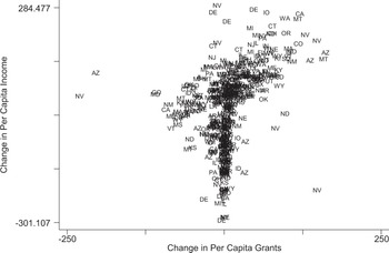
ANNUAL CHANGES IN PER CAPITA NEW DEAL GRANTS PLOTTED AGAINST CHANGES IN PER CAPITA PERSONAL INCOME FOR THE YEARS 1930 THROUGH 1940 BY STATE IN 1967 DOLLARS

Sources: See Data Appendix.

Figure 2 shows the large variation in the annual changes in per capita nontransfer federal grants plotted against per capita nontransfer income across states for the years 1930 through 1940, all measured in 1967 dollars. The changes over time within states after controlling for national shocks in each year are the source of variation used to identify the multipliers.

FEDERAL TAX POLICY IN THE 1930S

In the 1930s federal tax rates were the same across all states for each activity in each year. However, the tax structure during the 1930s was quite different from the post-war economy, in which the vast majority of internal tax revenues come from taxes on income in the form of corporate, personal, and employment (social security and unemployment insurance) taxes. Between 1930 and 1940 the sources of federal revenue shifted dramatically away from income taxes toward excise taxes. Less than 10 percent of households earned enough to pay personal income taxes before 1940. In 1930 personal income taxes accounted for 38 percent of total internal revenue and corporate income taxes composed 42 percent. The Tax Revenue Act of 1932 led to several major changes. Even though income tax rates were increased, the share of revenue from personal income taxes fell markedly to 16 percent in 1934 and 18 percent in 1940, while the share from corporate income taxes fell to 15 percent in 1934 before rising to 21 percent in 1940. The big revenue sources that arose from the 1932 tax changes were an expansion in excise taxes to cover manufactures of autos, tires, gasoline, lubricants and taxes on pipelines, telephones, telegraphs, and electricity. The share of internal revenue from excise taxes rose from 19 percent in 1930 to 28 percent in 1933. In 1933 the Roosevelt administration added in processing taxes on agricultural goods, a capital stock tax and eliminated Prohibition. The excise tax share jumped to 48 percent in 1934. Over the rest of the decade the excise tax share fell back to 35 percent, although the share of the new revenues from alcohol taxes that were collected after Prohibition ended remained steady around 12 percent (Fishback Reference Fishback2010).Footnote ¹⁷

We deal with federal taxation in two ways. Since national tax rates were the same across all states, the simplest way is to incorporate year fixed effects that control for tax rate changes in a model of state per capita income as a function of national government spending per capita in the state. Essentially, the model shows the multiplier of federal spending for income after controlling for the fiscal drag created by the tax rate system. We also estimate the model with a dependent variable of per capita state income as a function of real per capita national government spending minus real per capita national taxes. This is the multiplier for income from federal government spending net of taxes.

ESTIMATION PROCEDURE

Despite the variety of theoretical models that generate income multipliers of government spending, their empirical estimation tends to be similar: reduced form models with a sparse set of correlates. To estimate the multiplier (β ₁), we use panel data methods with a measure of real per capita state income (y_it ) in state i and year t in 1967 dollars as the dependent variable as a function of a measure of real per capita federal spending in state i and year t (g_it ),

To control for exogenous omitted variables that might have influenced federal policy and state income, we include several vectors. A vector of extreme weather (W) variables—days with temperatures over 90, days with temperatures below 0, months of extreme or severe drought, and months of extreme or severe wetness, and precipitation—controls for the influence of these factors on crop production and prices in the farm sector, construction activity, and other activities where weather was a factor.Footnote ¹⁸ A vector of state fixed effects (S) controls for factors like geography, state constitutions, and the basic economic, cultural, and demographic structure of each state that did not change over time but varied across states. When the state fixed effects are added to the model, the variation that identifies the multiplier for federal funding (β ₁) is changes across time within the same state. A vector of year fixed effects (Y) controls for national changes in the economy that affected all states in each year, including monetary policy changes, changes in federal tax rates, the introduction and elimination of the National Recovery Administration, and other changes in national regulation. The addition of the year fixed effects to the state fixed effects specifications means that the multiplier is identified by variations within the same state over time after controlling for national shocks to the economy. The addition of a vector of state specific time trends (S∗t) controls for differences in the trend paths of economic activity in each state, including much of the shift away from state budget deficits in the early 1930s to budget surpluses in the late 1930s.Footnote ¹⁹ Under the complete model specification the identification of the multiplier comes from deviations from trend across time within the states after controlling for nation-wide shocks.

As an alternative way to control for state fixed effects, the model can also be estimated in year-to-year first differences. The year effects in the first difference model still serve the same purpose of controlling for nationwide shocks in each year. In the difference model state time trends are controlled with the addition of state fixed effects. Both methods lead to unbiased and consistent estimates of the multiplier in large samples, but the standard errors are more efficiently estimated by the difference estimation if there is serial correlation (Wooldridge Reference Wooldridge2006, pp. 491–92). Since the sample is relatively small with 48 states for 11 years each, we report both sets of estimates.Footnote ²⁰

There still remains the possibility of biases from simultaneity and endogeneity. Ample literature on the geographic distribution of New Deal spending shows that the Roosevelt Administration tended to distribute more New Deal grants to areas where income was declining (see Wallis Reference Wallis1998; Fleck Reference Fleck2008; Fishback, Kantor, and Wallis Reference Fishback, Kantor and Wallis2002; Neumann, Fishback, and Kantor Reference Johnson, Fishback and Kantor2010). This tendency imparts a negative bias to the multiplier coefficient. To eliminate the biases arising from the issues described above, we follow an instrumental variable strategy. To be effective, the instrument must vary annually both across time and across space and be strongly correlated with the measures of federal government funds but not with the error term in the final-stage equation.

The instrument logic starts with the shift-share logic used by Wallis and Benjamin (Reference Wallis and Benjamin1981), Nakamura and Steinsson (Reference Nakamura and Steinsson2014), and many others. Establish a baseline structure for the types of federal spending from an earlier period in each state. Then use changes in national spending for each type of federal spending multiplied by the earlier state shares to develop an estimate of state spending in each year that is driven purely by national changes.

One key question that arises is whether the national totals in each category are correlated with the error in each specific state after controlling for weather fluctuations and state and year fixed effects. There are two reasons to believe that there is a lack of correlation. First, each state was a small share of the national economy. New York received the largest share of federal grants at 9.6 percent. Second, the federal government since 1789 had treated employment and labor policies and poverty as exclusively a state and local issue. The stated reason for the federal government getting involved with these programs is that the Great Depression was a national problem. The new programs of the 1930s were the federal relief programs, the additional public works programs, and the AAA farm program, and these accounted for the lion's share of federal spending in the 1930s. When reading through the appropriations for these programs, the national totals for appropriations were typically very large round numbers. There is no doubt that the President and members of Congress tried to influence the distribution of the spending across states once the total was set. However, the process of setting the total required majority votes in the House of Representatives and Senate and avoiding Presidential vetoes. This process would have muted the impact of any one state's representatives’ attempts to increase the national total to benefit his state. Such a move would have likely involved extensive horse-trading among enough Congressmen that it is the collection of a large number of states that was determining the national total.

To avoid further correlation of the error in state i and year t with the national total, we took another step with the instrument in which we construct a “moat” around each state that includes the state's own regions and neighboring regions. We then use the national totals from outside that moat for the shift-share calculations of the instrument. The moat is constructed to put substantial distance between the observation state and the area being used for the national total. For New England, for example, the moat includes any states in New England, the Mid-Atlantic, the East North Central, or the states of Virginia, Maryland, Kentucky, and West Virginia. The moat areas are large enough that they could come close to becoming self-contained economies.Footnote ²¹

Another question is whether the state shares for 1925–1928 are correlated with fluctuations in income in the specific state in the 1930s. That seems unlikely even when we do not include state fixed effects in the analysis. We have run regressions on the distributions of state funds across states and time in separate panels for 1923–1929, 1930–1933, and 1934–1939 based on presidential administrations. A number of factors that drove the distribution across states and time in the 1930s did not drive the distribution in the 1920s. Once we include state fixed effects in the analysis for the 1930s, it reduces even further the likelihood that the state shares in the 1920s were correlated with the errors in the final stage regression in the 1930s because it would require the deviation from the state average for a specific year in the 1930s to be correlated with a state share of federal funds in the mid-1920s.

For the instrument to be correlated with the error term in state i in year t, the error would have to be correlated with either the distribution across states in 1928 after controlling for time-invariant features of the state and/or correlated with the total federal spending in other parts of the country that are well outside a large multi-region and roughly self-contained economic area surrounding the state after controlling for national shocks and for weather shocks within the state.

ESTIMATES OF INCOME MULTIPLIERS

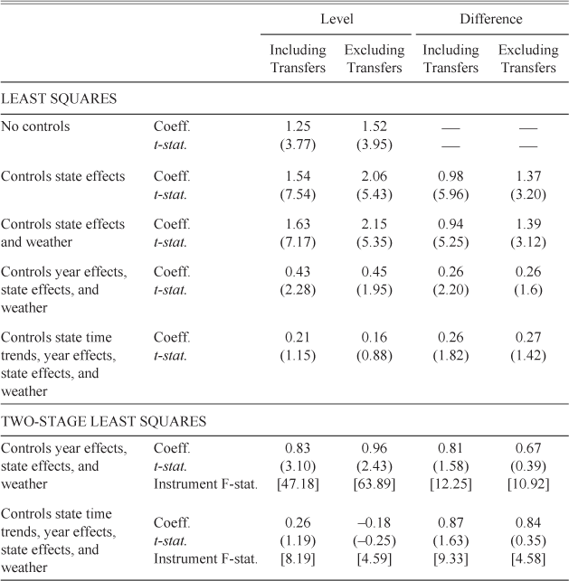
The state personal incomes are reported on a calendar year basis, while the federal spending is reported on a fiscal year basis, covering the period from 1 July in year t – 1 to 30 June in year t. This automatically imparts a one-half year lag into the model.Footnote ²² Table 2 shows coefficients and standard errors from a series of estimations with per capita state personal income in 1967 dollars as a function of per capita estimates of federal government fiscal activity in the state. Estimates using the level and first difference specifications are reported when per capita incomes and grants include transfers (the first two columns) and when they exclude transfers (third and fourth columns). They show the coefficients and standard errors for per capita federal grants in the level specification as correlates are added cumulatively, and the second column shows the results for the differenced model. Each row matches logical equivalents for controls, such that the second row shows the results from a level equation controlling for state fixed effects on the same line as the differenced equation without fixed effects.

Table 2

ESTIMATES OF DOLLAR-FOR-DOLLAR EFFECT OF PER CAPITA GRANTS ON STATE PER CAPITA INCOME, 1930–1940

Notes:

Including transfers means that both income and grants included transfers, excluding transfers means that neither included transfers. This is a balanced panel with information for 48 states for each year from 1930 through 1940. For the calculations of t-statistics, standard errors are based on White corrections using the robust command with standard errors clustered at the state level. The instrument F-statistic is the Kleibergen-Paap rank Wald (KP) F statistic.

Sources:

See Data Appendix.

The least squares estimate of the multiplier without controls is 1.25 when transfers are included in both personal income and government grants and 1.52 without them. Adding controls for time-invariant features of the states increases the multipliers, while adding controls for weather leads to only minor adjustments. The addition of year fixed effects controls for the national shocks related to the major changes in monetary policy during the 1930s as well as changes like the National Recovery Administration and federal policies toward unions that altered the structure of many product and labor markets. Once the year fixed effects control for these factors, the multiplier is cut below 0.5. When we add controls for state time trends, the variation identifying the multiplier is deviations from trend over time within the states after controlling for national shocks, and the multiplier falls below 0.3.

IV Estimates in Levels with Fixed Effects

The estimation procedures that lead to the most positive estimates for the New Deal are the IV estimates when the data is set up in levels and state and year fixed effects are included. The instruments are strong, as the Kleibergen-Paap F-statistics in Tables Table 2 through 4 are generally much larger than 10, the rule-of-thumb value used in most papers (Kleibergen and Paap Reference Kleibergen and Paap2006). When state-specific time trends are incorporated, the F-statistics are much lower, and the estimates likely have more weak instrument bias. As a result, we focus on models with only controls for state and year fixed effects in our discussion.

The multiplier estimate is 0.83 when transfers are included and 0.96 when transfers are excluded and both are statistically significantly different from zero.Footnote ²³ The estimates are substantially below the recent estimate of 1.5 by Nakamura and Steinsson (Reference Nakamura and Steinsson2014) for military spending and somewhat above the estimates for government spending found across countries by Kraay (Reference Kraay2012). One reason may be differences in the type of spending. Nakamura and Steinsson focus on military expenditures while the New Deal spending ranges across a wide range of programs, including the AAA farm program, which has a natural crowding out feature. Meanwhile, Kraay's estimates also cover a wide range of public works spending.

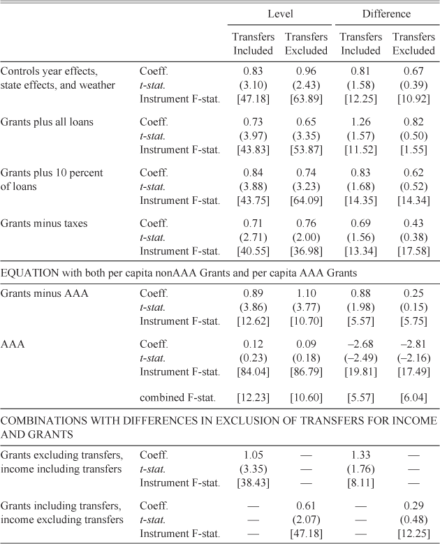
The point estimates of multipliers for different federal funding measures during the 1930s are shown in Table 3. All but the estimate for AAA grants are statistically significantly different from zero. Whether we add in loans, or subtract taxes, or mix and match the exclusion of transfers from income or from the federal funds at the bottom of the table, the multiplier estimates in the level specifications are all between 0.61 and 1.05 and we cannot reject the hypothesis that the multiplier is one.

Table 3

IV ESTIMATES OF DOLLAR-FOR-DOLLAR EFFECT OF PER CAPITA GOVERNMENT FUNDING ON STATE PER CAPITA INCOME, 1930–1940

Notes:

All analyses are from individual regressions except for the nonAAA and AAA results, which are estimated in the same regression. All equations include state and year fixed effects and weather measures. The instrument F-statistic is the Kleibergen-Paap rank Wald (KP) F statistic. When loans are included, missing data leads to the loss of 1940 observations from the panel. In the top two-thirds of the table, including transfers means that both income and government funds include transfers, excluding transfers means both exclude transfers.

Sources:

See Data Appendix.

Given that the AAA farm grants were designed to take land out of production, we expected that the nonAAA grants would have stronger positive effects than all grants and that the AAA potentially had negative effects on income. The multiplier for the nonAAA grants is somewhat larger than for all grants, 0.89 versus 0.83 when transfers are included and 1.10 versus 0.96 when they are excluded. However, the multiplier estimates for AAA grants are both below 0.13 and neither is statistically significant.

The findings of the positive effect of nonAAA grants and weak effects of AAA grants are similar to Fishback, Horrace, and Kantor's (Reference Fishback, Horrace and Kantor2005, Reference Fishback, Horrace and Kantor2006) findings using county level data. Using a different instrument strategy, they find that public works and relief were associated with higher retail sales and net in-migration and that AAA grants were associated with slightly lower retail sales and net out-migration. The payments would have benefited farm owners and those tenants who received a share of the AAA payments. On the other hand, the reduction in the demand for farm labor would have reduced wages and employment for farm workers and sharecroppers.Footnote ²⁴ In fact, Briggs Depew, Fishback, and Paul Rhode (Reference Depew, Fishback and Rhode2013) find that AAA grants led to sharp decline in the number of share tenants and croppers between 1930 and 1935.

Even though the results in Table 3 show variations in the multiplier for different forms of spending, it is important to note that the standard errors of the estimates for total spending and nonAAA spending are large enough that we cannot reject a multiplier of one for nearly every estimate.

IV Estimates with First Differences and Year Fixed Effects

A less positive picture of the multiplier is painted by the estimates when we estimate the model in first differences with year fixed effects. The point estimates in Tables 2 and 3 for the differenced model with year fixed effects are similar to the ones for the levels model with state and year fixed effects. However, the standard errors for the estimates are larger, such that only three of the coefficients from the differenced models are statistically significantly different from zero at the 10 percent level, and one of those is the negative coefficient of income with respect to AAA grants in Table 4.

Table 4

IV ESTIMATES OF ELASTICITY OF VARIABLE WITH RESPECT TO NONTRANSFER GOVERNMENT GRANTS

Notes:

See notes in Tables 2 and 3.

Sources:

See Data Appendix.

There are several potential reasons for why the standard errors using the differenced model would be larger. One possibility is that the instruments are weaker in the differenced model. Even though the Kliebergen-Paap F-statistics in Tables 2 through 4 are smaller for the differenced estimates, we do not believe that this is the primary source of the problem because most still exceed the ten rule-of-thumb value.

Michael Baker, Dwayne Benjamin, and Shuchita Stanger (Reference Baker, Benjamin and Stanger1999) suggest that the first-difference models tend to be more sensitive to specifying the lag structure correctly. When we tried using a model with second-differences, the results were similar to the first-differenced results. We have also explored incorporating lagged spending in the levels model, but the coefficient of lagged spending was very small and not statistically significant.

Another potential reason is problems with measurement error and errors in variables. The measurement error is smaller when transfers are included in the per capita income measure from Creamer and Merwin (Reference Creamer and Merwin1942) than in the measure without transfers because we could only make imperfect adjustments to obtain the nontransfer estimates. As a result, the estimates including transfers tend to have smaller standard errors for the estimates than the estimates without transfers. Zvi Griliches and Jerry Hausman (Reference Griliches and Hausman1986) suggest that the first-differenced models may lead to more problems with errors in variables than the use of level estimates. This seems to fit the pattern here, because the differenced specifications have much larger standard errors than their matching level specifications. Whatever the reason for the difference in the size of the estimated standard errors, we felt it important to follow Jeffrey Wooldridge's (Reference Wooldridge2006, pp. 491–92) suggestion to report estimates from both the level and differenced model when they differ.

THE IMPACT OF FEDERAL GRANTS ON AUTOMOBILE REGISTRATIONS AND EMPLOYMENT

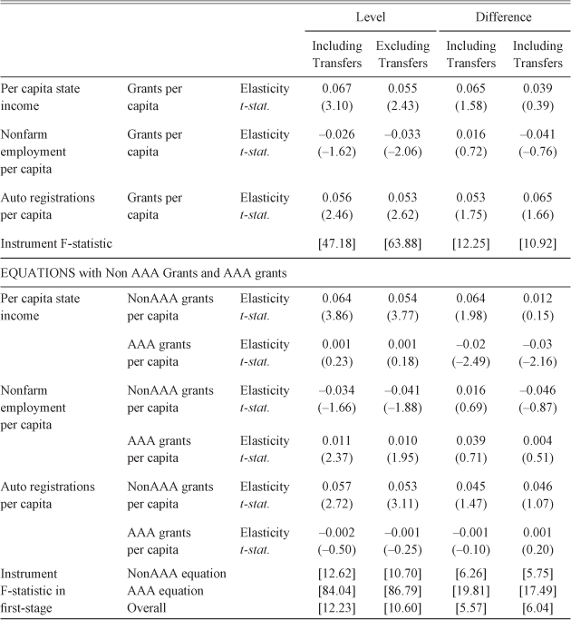
Discussions of federal spending have often focused on consumption and on private employment. We can measure the impact on consumption of a major durable good using data on per capita automobile registrations with the states. We can also measure the impact on private employment per capita using indices of nonfarm employment per capita, which were compiled by the Bureau of Labor Statistics and adjusted for benchmarks by John Wallis (Reference Fishback, Kantor and Wallis1989). These measures are not in dollar terms; therefore, Table 4 shows the elasticities of each measure with respect to federal grants without transfers. For comparisons, Table 4 also shows the elasticities calculated at the sample means for per capita state income. The multiplier estimates ranging from 0.67 to 0.96 in Table 3 translate into elasticities of per capita income with respect to per capita grants that range from 0.039 to 0.067.

The distribution of government funds had strong effects on automobile registrations per capita. The level and difference analyses controlling for state and year fixed effects estimate elasticities of 0.05 and 0.06, which are comparable to the elasticities for per capita income. To gain a rough idea of how the elasticity of per capita auto registrations can be translated into dollars of consumption, value each car at the price of a new Ford in 1934, which was about $500 then and $1,247 when adjusted to the 1967 CPI values used to control for the price level. An additional dollar of federal spending raised the value of car registrations by between 14 and 16 cents.

As was the case for per capita income, the nonAAA grant spending had a much stronger effect on auto registrations than the AAA grants did. The per capita auto registration elasticity for nonAAA grants per capita in the level analyses were statistically significant values near 0.055, while the AAA elasticity was negative and much smaller at around −0.002 or −0.001. In the difference analysis the nonAAA elasticity is around 0.045, while the AAA elasticity ranges between 0.001 and −0.001.

In both the 1930s and the 2000s it was hoped that more federal grants would lead to spillover increases in private employment. The various studies of this issue cited in the literature review find little or no positive effect of relief programs. The results here are similar. The estimates for elasticities of nonfarm employment per capita with respect to all grants are negative in three of the specifications and the small positive estimate of 0.016 is not statistically significant. These all imply some crowding out of private employment, despite the high levels of unemployment.^{25, 26} When the effects of nonAAA and AAA grants are estimate separately, the coefficients for the nonAAA grants are similar to the ones for all grants. On the other hand, the coefficients on the AAA grants are positive and two are statistically significant. This positive effect may have been driven by a surge in labor supply that was caused when the AAA led to the reduction of opportunities for share tenants, croppers, and farm workers (Depew, Fishback, and Rhode Reference Cullen and Fishback2013).

CONCLUSION

If there was any time to expect a large peace-time state multiplier from federal spending in the states, it might well have been during the period from 1930 through 1940. Interest rates were at or near the zero bound for nearly the entire decade and unemployment of labor and capital was rampant throughout the decade. The state multiplier captures the direct gain to a state from increased federal spending in the state. Without using instruments state multiplier estimates controlling for weather shocks, state and year fixed effects, and in some cases state-specific time trend imply that the state personal income multipliers were in the 0.1 to 0.5 range. These estimates are likely biased downward due to endogeneity arising from the Roosevelt administration's attempts to distribute federal funds in response to drops in economic activity.

We estimated a series of per capita income multipliers using different definitions of government spending. The IV income multiplier estimates ranged from 0.4 to 0.96 in level and first-difference analyses that control for state and year fixed effects. We can reject the hypothesis of a zero multiplier in the level analysis with state and year fixed effects. However, the estimated standard errors in the differenced analysis with year fixed effects are large enough in most cases we cannot reject a zero multiplier. Generally, we cannot reject the hypothesis that the state multiplier for federal spending in the 1930s was one. When the grants are split into two major categories—(1) AAA farm grants and (2) public works and relief and other nonAAA grants, the AAA grants had much smaller effect than the remaining grants. The difference likely came about because the AAA grants paid farmers to take land out of production, which led to negative consequences for farm workers, croppers, and tenants, while benefiting farm owners (see also Fishback, Horrace, and Kantor Reference Fishback, Horrace and Kantor2005, Reference Fishback, Horrace and Kantor2006; Depew, Fishback, and Rhode Reference Depew, Fishback and Rhode2013).

In the modern era it is often claimed that tax rebates and stimulus spending may lead to increased net income but not stimulate consumption. In the 1930s at least some of the increased income from federal grant spending translated into higher consumption, as grants and nonAAA grants had strong positive effects on automobile registrations.

On the other hand, nonAAA grants had no positive effect on private employment in the states. This finding is consistent with findings of other studies on the effect of New Deal relief programs on private employment.Footnote ²⁷ All of these studies are consistent with the fact that unemployment rates remained high throughout the 1930s even during periods when real GDP was growing rapidly from its trough. To the extent that findings for the 1930s are relevant to the modern era, the lack of positive effects of public works and relief spending raise some questions about how successful such expanded spending will be at the state level in the modern era. In fact, the literature on the modern employment effects of federal stimulus at the subnational level contains examples of both negative and positive effects of fiscal spending on local employment (Suarez Serrato and Wingender Reference Serrato, Suarez and Wingender2010; Wilson Reference Wilson2012; Cohen, Coval, and Malloy Reference Cohen, Coval and Malloy2011).