1. Introduction
The winds and tides inject kinetic energy into the ocean’s internal wave field (Ferrari & Wunsch Reference Ferrari and Wunsch2009). Part of this kinetic energy can be converted to background potential energy when internal waves break and mix density. This process is thought to play an essential role in resupplying the potential energy lost by the meridional overturning circulation (Wunsch & Ferrari Reference Wunsch and Ferrari2004). Knowledge of why and where internal waves break is thus needed to understand how the ocean’s global energy balance is closed. It is thought that the ocean’s boundaries are especially effective at converting large-scale internal waves into mixing-prone internal waves (for a review, see Garrett & Kunze Reference Garrett and Kunze2007). This fact is explained by the peculiar propagation properties of internal waves.
Internal waves propagate in fluids with stable stratification and/or that rotate. While the restoring force in the latter is quantified by the Coriolis frequency
 $f$
, in the former it is quantified by the Brunt-Väisälä, or buoyancy, frequency
 $N=\sqrt{-(g/{\it\rho}_{0})\partial _{z}\overline{{\it\rho}}}$
, where
 $g$
is the gravitational acceleration,
 ${\it\rho}_{0}$
a constant reference density, and
 $\overline{{\it\rho}}$
the unperturbed density field. The dispersion relation of internal waves in such a fluid is
 ${\it\omega}^{2}=N^{2}\sin ^{2}{\it\beta}+f^{2}\cos ^{2}{\it\beta}$
, where
 ${\it\omega}$
is the wave frequency and
 ${\it\beta}$
is the angle of the group velocity vector with respect to the horizontal plane. Following this dispersion relation, waves radiated from a point source oscillating at a frequency
 ${\it\omega}$
, with
 $|\,f|<{\it\omega}<N$
, in a fluid confined in a vertical plane will propagate in the four directions allowed by the above dispersion relation, forming a symmetric Saint-Andrews-cross pattern (Mowbray & Rarity Reference Mowbray and Rarity1967).
As first noted by Phillips (Reference Phillips1966), the form of the dispersion relation leads to a peculiar wave reflection at a wall inclined with respect to the gravity vector: because
 ${\it\omega}$
is preserved upon reflection, the angle
 ${\it\beta}$
is preserved as well. Three scenarios for such reflections exist: (i) the wall is shallower than
 ${\it\beta}$
, in which case the waves keep their horizontal propagation direction, but reverse their vertical propagation; (ii) the wall is steeper than
 ${\it\beta}$
, in which case the opposite happens; (iii) the wall angle is equal to
 ${\it\beta}$
and the wave energy is focused to a line, which represents a singularity of the linear, inviscid equations of wave propagation. The latter is called ‘critical reflection’ and divides the frequency parameter space into two regimes, (i) and (ii) being most often referred to as ‘sub-’ and ‘super-critical’, respectively, although unfortunately, some authors use the opposite convention. Sub- and super-critical reflections are also less frequently described as ‘forward’ and ‘backward’, respectively (e.g. Javam, Imberger & Armfield Reference Javam, Imberger and Armfield1999). This refers to the continuity or reversal of the wave propagation in the horizontal, respectively, and will be used throughout this article. Critical and near-critical reflections induce wave focusing, which eventually leads to enhanced dissipation.
The properties of internal waves described above form what we will call ‘classical’ reflection. When the horizontal projection of the Earth’s rotation vector cannot be ignored, i.e. the ‘non-traditional’ case, as reviewed by Gerkema et al. (Reference Gerkema, Zimmerman, Maas and van Haren2008), for example in weakly stratified parts of the deep ocean, even horizontal fluid boundaries can host similar effects. The horizontal/vertical symmetry is broken by the tilted rotation vector of the Earth, and pure inertial waves (
 ${\it\omega}=f$
) either can have
 ${\it\beta}=0$
, as in the classical case, or can propagate at an angle with respect to the horizontal. As a consequence, downward-propagating inertial waves can experience critical reflections from flat bottoms (Gerkema & Shrira Reference Gerkema and Shrira2005; Winters, Bouruet-Aubertot & Gerkema Reference Winters, Bouruet-Aubertot and Gerkema2011). More generally, non-traditional effects modify the geographic distribution of critical slopes for near-inertial waves (NIWs), and increase the overall probability of critical reflections occurring (Gerkema & Shrira Reference Gerkema and Shrira2006).
As previously noticed by Whitt & Thomas (Reference Whitt and Thomas2013), a strong analogy can also be drawn between the propagation of NIWs in the non-traditional case and of NIWs in fronts. An ocean front is a sharp feature consisting of a large horizontal density gradient and currents with strong vertical shear. This shear imparts a horizontal component to the absolute vorticity of the fluid, analogous to the non-traditional case, and hence allows similar wave physics. Frontal currents are characterized by Rossby and Richardson numbers that are order one and thus categorize fronts as sub-mesoscale structures, for which the geostrophic balance is less dominant than for the mesoscale eddy field. As a consequence, vertical velocities found in fronts tend to be an order of magnitude larger than those found in mesoscale structures, which makes fronts particularly important for the sequestration of gases and heat in the ocean and for supplying nutrients to fuel the growth of phytoplankton (see e.g. Thomas, Tandon & Mahadevan Reference Thomas, Tandon, Mahadevan, Hecht and Hasumi2008; Klein & Lapeyre Reference Klein and Lapeyre2009). Recent theoretical developments have highlighted the role of internal waves in sub-mesoscale and frontal dynamics (Thomas Reference Thomas2012; Whitt & Thomas Reference Whitt and Thomas2013; Thomas & Taylor Reference Thomas and Taylor2014). This work builds on of previous studies that have found that energy in NIWs accumulates near ocean fronts (e.g. Kunze & Sanford Reference Kunze and Sanford1984; Kunze, Schmitt & Toole Reference Kunze, Schmitt and Toole1995; Marshall et al. Reference Marshall, Andersson, Bates, Dewar, Doney, Edson, Ferrari, Forget, Fratantoni, Gregg, Joyce, Kelly, Lozier, Lumpkin, Maze, Palter, Samelson, Silverthorne, Skyllingstad, Straneo, Talley, Thomas, Toole and Weller2009).
The combination of vertical and lateral density gradients at a front results in sloping isopycnal surfaces, which once again breaks the vertical/horizontal symmetry found in the classical theory. At first glance, the situation might appear analogous to the case where the direction of the gravity vector is tilted at an angle, approximately equal to the background isopycnal angle. For this scenario, the internal wave’s Saint-Andrews-cross pattern would tilt with the same angle, and interestingly, horizontal boundaries like the ocean surface would become equivalent to a sloping wall in the classical case. To be complete however, one has to take into account the additional effect of the horizontal vorticity induced by the thermal wind shear, which further modifies propagation angles. Nonetheless, this simple analogy leads one to expect the existence of frontal equivalents of classical forward and backward reflection, separated by a critical reflection.
In this article, we will demonstrate that this is the case. The linear theoretical basis for this finding is described in § 2. In order to illustrate the theory and go beyond inviscid, linear arguments, we conduct non-hydrostatic, Boussinesq numerical experiments and their configurations are described in § 3. In § 4, we conduct linear numerical simulations which illustrate the basic physics of the phenomenon. Near-critical, nonlinear NIW reflections are then studied numerically in § 5, followed by their critical equivalent for pure inertial waves in § 6. Conclusions and further insights about the implications for more realistic oceanic fronts are then presented in § 7.
2. Reflection of near-inertial waves in a front from a horizontal boundary
2.1. Frontal flow
We consider an idealized ocean front in geostrophic and hydrostatic balance, characterized by a stable vertical density gradient as well as a horizontal density gradient in thermal wind balance. We orient the Cartesian coordinate axes such that
 $z$
is the vertical coordinate,
 $y$
the along-front direction and
 $x$
the (horizontal) across-front direction. We will hereafter neglect all along-front variations (
 $\partial _{y}\equiv 0$
), which is sufficient to capture the basic physics at play. We can then write the density field as
 $$\begin{eqnarray}{\it\rho}(x,z,t)={\it\rho}_{0}+\overline{{\it\rho}}(x,z)+{\it\rho}^{\prime }(x,z,t),\end{eqnarray}$$
where
 ${\it\rho}_{0}$
is a reference density,
 ${\it\rho}_{0}+\overline{{\it\rho}}$
the frontal density field in thermal wind balance, and
 ${\it\rho}^{\prime }$
the density perturbation. Because the ocean is usually characterized by
 $\overline{{\it\rho}}+{\it\rho}^{\prime }\ll {\it\rho}_{0}$
, we use the Boussinesq approximation, under which the density gradients are measured by the quantities
 $(S^{2},N^{2})=-g(\overline{{\it\rho}}_{x},\overline{{\it\rho}}_{z})/{\it\rho}_{0}$
, where lettered subscripts denote partial derivatives. We further assume that
 $S$
and
 $N$
are constant in space and time. Geostrophy implies the existence of a thermal wind
 $\overline{v}(z)$
in the along-front (
 $y$
) direction such that
 $$\begin{eqnarray}\overline{v}_{z}=S^{2}/f\quad \text{(thermal wind balance)}.\end{eqnarray}$$
Because oceanic fronts are typically much narrower than
 $O(100~\text{km})$
, we take
 $f$
to be constant. Finally, we associate the thermal wind shear with a Richardson number
 $\overline{\mathit{Ri}}$
:
 $$\begin{eqnarray}\overline{\mathit{Ri}}=N^{2}/|\overline{v}_{z}|^{2}=f^{2}N^{2}/S^{4}\end{eqnarray}$$
and assume that
 $\overline{\mathit{Ri}}>1$
, so that the flow is stable to symmetric instability (Haine & Marshall Reference Haine and Marshall1998).
The features described so far will hereafter be referred to as the ‘frontal flow’. To put some numbers on the parameters of the frontal flow, we draw our inspiration from the North Wall of the winter-time Gulf Stream, where Thomas et al. (Reference Thomas, Taylor, Ferrari and Joyce2013) report values of
 $S^{2}\approx 5\times 10^{-7}~\text{s}^{-2}$
. The North Wall of the Gulf Stream consists of a mid-latitude (
 $\,f\approx 10^{-4}~\text{s}^{-1}$
), strong front characterized by
 $\overline{\mathit{Ri}}\approx 1$
, which implies
 $N^{2}\approx 2.5\times 10^{-5}~\text{s}^{-2}$
and that the isopycnal slope is
 $S^{2}/N^{2}\approx 2\,\%$
. In this article, we use a similar value (
 $S^{2}/N^{2}\approx 1\,\%$
, cf. § 3.1).
2.2. Internal wave propagation in a front
We now consider perturbations relative to the frontal flow, that are small enough to be well described by the linearized Boussinesq equations. In the present section, we also consider NIWs, namely perturbations of low enough frequency for vertical accelerations to be neglected and for which the hydrostatic approximation can be used:
 $$\begin{eqnarray}\displaystyle & \displaystyle \boldsymbol{u}_{t}^{h}+f\hat{\boldsymbol{z}}\times \boldsymbol{u}+(S^{2}/f)w\hat{\boldsymbol{y}}-b\hat{\boldsymbol{z}}+\boldsymbol{{\rm\nabla}}p=0, & \displaystyle\end{eqnarray}$$
 $$\begin{eqnarray}\displaystyle & \displaystyle b_{t}+S^{2}u+N^{2}w=0, & \displaystyle\end{eqnarray}$$
 $$\begin{eqnarray}\displaystyle & \displaystyle \boldsymbol{{\rm\nabla}}\boldsymbol{\cdot }\boldsymbol{u}=0. & \displaystyle\end{eqnarray}$$
 $\boldsymbol{u}^{h}=(u,v,0)$
is the horizontal velocity perturbations vector and its Cartesian components,
 $\boldsymbol{u}=(u,v,w)$
the full perturbations velocity vector,
 $\hat{\boldsymbol{y}}$
the along-front unit vector (we define
 $\hat{\boldsymbol{x}}$
and
 $\hat{\boldsymbol{z}}$
similarly),
 $b=-g{\it\rho}^{\prime }/{\it\rho}_{0}$
the buoyancy fluctuations and
 $p$
the scaled pressure.
It is possible to reduce the above system of equations to a single equation using the perturbation stream function
 ${\it\psi}$
, defined by
 $(u,w)=(-{\it\psi}_{z},{\it\psi}_{x})$
, yielding the Eliassen–Sawyer equation (cf. e.g. Mooers Reference Mooers1975; Plougonven & Zeitlin Reference Plougonven and Zeitlin2005; Whitt & Thomas Reference Whitt and Thomas2013):
 $$\begin{eqnarray}\left(\,f^{2}+\partial _{tt}\right){\it\psi}_{zz}-2S^{2}{\it\psi}_{xz}+N^{2}{\it\psi}_{xx}=0.\end{eqnarray}$$
Let us now assume a perturbation in the form of a plane wave, namely
 ${\it\psi}$
is proportional to
 $\text{exp}(\text{i}(-{\it\alpha}mx+mz-{\it\omega}t))$
, where
 $\boldsymbol{k}=(-{\it\alpha}m,0,m)$
is the wavevector. Substituting in (2.5) yields the hydrostatic dispersion relation of internal waves in fronts:
 $$\begin{eqnarray}{\it\omega}^{2}({\it\alpha})=f^{2}+{\it\alpha}^{2}N^{2}+2{\it\alpha}S^{2}.\end{eqnarray}$$
The equation above differs from the standard dispersion relation by the term proportional to
 $S^{2}$
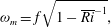
. We summarize here a few implications of this new additional term and refer readers to Mooers (Reference Mooers1975) and Whitt & Thomas (Reference Whitt and Thomas2013) for further details and derivations. One implication is that the minimum wave frequency allowed by the dispersion relation,
 ${\it\omega}_{m}$
, is lower than
 $f$
, namely:
 $$\begin{eqnarray}{\it\omega}_{m}=f\sqrt{1-\overline{\mathit{Ri }}^{-1}},\end{eqnarray}$$
which is obtained when
 ${\it\alpha}=-S^{2}/N^{2}$
, i.e. when the phase lines, whose slopes are equal to
 ${\it\alpha}$
, run parallel to isopycnals and the wavevector points perpendicular to isopycnals. Another consequence is that as
 $|S^{2}|$
increases, the classical Saint-Andrews-cross radiation pattern gives way to an inclined cross and we now have two characteristics with different inclinations
 ${\it\alpha}_{{\it\omega}}^{+}$
and
 ${\it\alpha}_{{\it\omega}}^{-}$
, hereafter referred to as steep and shallow, respectively:
 $$\begin{eqnarray}{\it\alpha}_{{\it\omega}}^{\pm }=-\frac{S^{2}}{N^{2}}\mp \sqrt{\frac{{\it\omega}^{2}-{\it\omega}_{m}^{2}}{N^{2}}}=-\frac{f}{N}\left(\frac{1}{\sqrt{\overline{\mathit{Ri}}}}\pm \sqrt{\frac{1}{\overline{\mathit{Ri}}}+\frac{{\it\omega}^{2}}{f^{2}}-1}\right).\end{eqnarray}$$
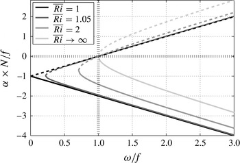
We plot values of
 ${\it\alpha}^{\pm }$
as a function of
 ${\it\omega}/f$
in figure 1 for a few values of
 $\overline{\mathit{Ri}}$
(see also figure 8 of Whitt & Thomas (Reference Whitt and Thomas2013)).
Normalized characteristic slopes
 ${\it\alpha}^{+}$
(solid) and
 ${\it\alpha}^{-}$
(dashed) as functions of frequency, for different values of
 $\overline{\mathit{Ri}}$
. Recall that
 $\overline{\mathit{Ri}}\rightarrow \infty$
corresponds to the classical,
 $S^{2}=0$
case. Hatched lines mark the
 ${\it\alpha}=0$
and
 ${\it\omega}=f$
locations.

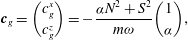
Differentiating equation (2.6) in wavenumber space yields the group velocity:
 $$\begin{eqnarray}\boldsymbol{c}_{g}=\binom{c_{g}^{x}}{c_{g}^{z}}=-\frac{{\it\alpha}N^{2}+S^{2}}{m{\it\omega}}\binom{1}{{\it\alpha}},\end{eqnarray}$$
which shows that wave energy propagates along vectors of slope
 ${\bf\alpha}$
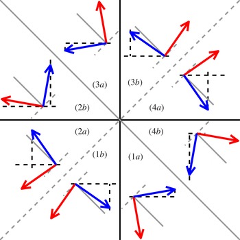
, namely along characteristics. Contrary to the classical case, the radiation diagram of internal waves cannot be split into four quadrants separating upward- and downward-, leftward- and rightward-propagating waves anymore. Nor is it sufficient to simply rotate the four quadrants to align their boundaries along iso- and diapycnal directions, since the presence of the flat ocean surface means that the up–down, left–right symmetry remains relevant to our problem. The radiation diagram is now divided into eight sectors, illustrated in figure 2. As in the classical case,
 $\boldsymbol{k}$
and
 $\boldsymbol{c}_{g}$
are perpendicular. Their respective projections onto the tangent of the background isopycnals, which is parallel to the vector
 $\hat{\boldsymbol{\imath }}=(1,-S^{2}/N^{2})$
, are:
 $$\begin{eqnarray}\boldsymbol{k}\boldsymbol{\cdot }\hat{\boldsymbol{\imath }}=-\!\left({\it\alpha}+\frac{S^{2}}{N^{2}}\right)m\quad \text{and}\quad \boldsymbol{c}_{g}\boldsymbol{\cdot }\hat{\boldsymbol{\imath }}=-\!\left({\it\alpha}+\frac{S^{2}}{N^{2}}\right)\left(1-\frac{{\it\alpha}S^{2}}{N^{2}}\right)\frac{N^{2}}{m{\it\omega}}\end{eqnarray}$$
which, like in the classical case, have the same signs because for NIWs under frontal oceanic conditions,
 $|{\it\alpha}S^{2}/N^{2}|\ll 1$
.
Configurations of group velocities (light grey arrows, red online) and wavevectors (dark grey arrows, blue online) for all possible wave propagation directions, under the hydrostatic approximation. Black lines (solid and dashed) mark the horizontal and vertical directions. Grey solid lines mark the background isopycnal slope
 $-S^{2}/N^{2}$
, while grey dashed lines mark the direction perpendicular to it. The isopycnal slope has been exaggerated for illustrative purposes. Each sector is identified in the inner circle of the figure (e.g. (1a)).

The present study revolves around the particular case where
 ${\it\omega}=f$
, for which (2.6) becomes:
 $$\begin{eqnarray}{\it\alpha}_{f}\left({\it\alpha}_{f}N^{2}+2S^{2}\right)=0.\end{eqnarray}$$
As is obvious from the above equation and noted by Whitt & Thomas (Reference Whitt and Thomas2013), for any given medium with parameters
 $N$
,
 $f$
and
 $S$
, horizontal characteristics (
 ${\it\alpha}_{f}=0$
) are always a solution, like in the classical case. However, in the
 $S=0$
case, the
 ${\it\alpha}_{f}=0$
solution is degenerate, i.e. the two characteristics collapse onto the horizontal. Here,
 ${\it\alpha}_{f}=0$
only corresponds to the shallow characteristic of slope
 ${\it\alpha}_{f}^{-}$
, while the steep characteristic has a slope
 ${\it\alpha}_{f}^{+}=-2S^{2}/N^{2}$
. Because energy propagates along characteristics, waves of frequency
 $f$
can have a finite vertical group velocity along the steep characteristic, or can have no vertical group velocity at all (along the shallow characteristic). While the latter is also the case in the classical,
 $S=0$
case, the former is unique to the frontal case. This has important implications for the reflection of NIWs in a front off the ocean surface.
2.3. Near-inertial wave reflection from the ocean surface
Indeed, imagine that waves oscillating at the frequency
 $f$
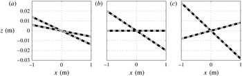
happen to propagate upwards, along steep characteristics. These waves will eventually encounter the ocean surface, which is horizontal and therefore aligns with the shallow characteristic. Their energy will accumulate under the surface in the same manner that energy can accumulate along sloping boundaries in classical critical reflection (Phillips Reference Phillips1966), or along flat surfaces in non-traditional cases (Gerkema & Shrira Reference Gerkema and Shrira2005). By analogy, we will qualify the present reflection as ‘critical’. The critical reflection separates the frequency space into two regions, those of ‘forward’ (
 ${\it\omega}>f$
) and of ‘backward’ (
 ${\it\omega}<f$
) reflections, as illustrated in figure 3. In both cases, when incident waves propagate along steep (shallow) characteristics, the reflection is (de-)focusing, i.e. ray tubes compress (expand). In the present work, we will only consider focusing reflections.
Schematic of forward (a), critical (b) and backward (c) focusing reflections at an ocean front. Grey lines are undisturbed isopycnals, dashed lines are characteristics along with their associated direction of propagation. (a)
 ${\it\omega}>f$
; (b)
 ${\it\omega}=f$
; (c)
 ${\it\omega}<f$
.

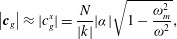
Similar to the classical case, described by e.g. Phillips (Reference Phillips1966) or Thorpe & Haines (Reference Thorpe and Haines1987), incident and reflected waves are bound by two constraints, namely that their frequency and along-boundary wavenumber are the same. Translated to the frontal case, the equivalent constraints are that incident and reflected waves share the same horizontal wavenumber
 $k$
, and that their slopes are symmetric around the isopycnal slope (cf. (2.8)). This implies that the magnitude of the group velocity:
 $$\begin{eqnarray}\left|\boldsymbol{c}_{g}\right|\approx |c_{g}^{x}|=\frac{N}{|k|}|{\it\alpha}|\sqrt{1-\frac{{\it\omega}_{m}^{2}}{{\it\omega}^{2}}},\end{eqnarray}$$
decreases upon focusing reflection since
 $|{\it\alpha}^{-}|<|{\it\alpha}^{+}|$
, which would reinforce the amplification of wave energy by the compression of ray tubes.
3. Set-up
3.1. Domain
We numerically simulate cases of critical, forward and backward reflections. As in the previous section, we assume a two-dimensional flow with no variations in the
 $y$
direction (
 $\partial _{y}\equiv 0$
). The domain has length
 $L=400~\text{m}$
and depth
 $H=50~\text{m}$
or
 $H=100~\text{m}$
, depending on the numerical simulation. We use a Coriolis parameter of
 $f=10^{-4}~\text{s}^{-1}$
, typical of mid-latitudes. The buoyancy gradient of the background flow is spatially uniform. The vertical gradient is the same for all simulations and equal to
 $N^{2}=10^{-4}~\text{s}^{-2}$
. For most of the experiments, a background lateral gradient of
 $S^{2}\approx 9.8\times 10^{-7}~\text{s}^{-2}$
(corresponding to
 $\overline{\mathit{Ri}}=1.05$
or
 $S^{2}/N^{2}\approx 1\,\%$
) is used. However, a couple of experiments with weaker lateral buoyancy gradients, i.e.
 $S^{2}\approx 7.1\times 10^{-7}$
and
 $5\times 10^{-7}~\text{s}^{-2}$
(
 $\overline{\mathit{Ri}}=2$
and 4, respectively) were performed and are described in § 4.1.
The domain is periodic in the
 $x$
direction. The surface of the ocean, located at
 $z=0$
, is modelled as a free-slip, rigid lid:
 $$\begin{eqnarray}\displaystyle & \displaystyle w|_{z=0}\equiv 0, & \displaystyle\end{eqnarray}$$
 $$\begin{eqnarray}\displaystyle & \displaystyle \left.(u_{z},v_{z}+\overline{v}_{z})\right|_{z=0}\equiv (0,0)\quad \Rightarrow \quad v_{z}|_{z=0}\equiv -S^{2}/f. & \displaystyle\end{eqnarray}$$
 $v$
requires a surface stress for the perturbation velocity
 $v$
in order to compensate for what Thomas & Rhines (Reference Thomas and Rhines2002) call the ‘geostrophic stress’, namely the stress induced by the thermal wind shear. We also set the buoyancy fluctuations to zero at the top of the domain, which amounts to setting the buoyancy at
 $z=0$
to a value, constant in time (but increasing with
 $x$
as
 $S^{2}x$
), which for the buoyancy perturbations, amounts to setting
 $$\begin{eqnarray}b|_{z=0}\equiv 0.\end{eqnarray}$$
We want to draw attention to the fact that this boundary condition is imposed by the numerical code, but is somewhat unphysical. Indeed, the condition ‘attaches’ isopycnals to given locations along the boundary. In the ocean, one would expect density perturbations to be advected along the boundary, which cannot happen here. In a companion article (N. Grisouard & L. N. Thomas, personal communication), we are able to analytically test the sensitivity of the flow to a no-flux boundary condition (
 $b_{z}|_{z=0}\equiv 0$
), and the results suggest that the conclusions of the present article will not be affected by the form of the boundary condition. Having said this, implementing a no-flux boundary condition is not necessarily realistic either, since the ocean surface is host to intense air–sea buoyancy fluxes.
We use the same boundary conditions for the bottom of the domain (
 $z=-H$
), although this boundary will play a limited role in the present study.
3.2. Equations solved
We use a modified version of the pseudo-spectral model of Winters, MacKinnon & Mills (Reference Winters, MacKinnon and Mills2004), which solves
 $$\begin{eqnarray}\displaystyle & \displaystyle \boldsymbol{u}_{t}+(\boldsymbol{u}\boldsymbol{\cdot }\boldsymbol{{\rm\nabla}})u+f\hat{\boldsymbol{z}}\times \boldsymbol{u}+(S^{2}/f)w\hat{\boldsymbol{y}}+\boldsymbol{{\rm\nabla}}p-b\hat{\boldsymbol{z}}=\mathscr{D}_{}\boldsymbol{u}+\boldsymbol{F}+G\hat{\boldsymbol{y}}, & \displaystyle\end{eqnarray}$$
 $$\begin{eqnarray}\displaystyle & \displaystyle b_{t}+(\boldsymbol{u}\boldsymbol{\cdot }\boldsymbol{{\rm\nabla}})b+S^{2}u+N^{2}w=\mathscr{D}_{}b+F_{4}, & \displaystyle\end{eqnarray}$$
 $$\begin{eqnarray}\displaystyle & \displaystyle \boldsymbol{{\rm\nabla}}\boldsymbol{\cdot }\boldsymbol{u}=0. & \displaystyle\end{eqnarray}$$
The dissipation operator is
 $\mathscr{D}_{}={\it\nu}^{z}\partial _{z}^{2}-{\it\nu}_{4}^{h}\partial _{x}^{4}$
, with
 ${\it\nu}^{z}$
the vertical viscosity and
 ${\it\nu}_{4}^{h}$
the horizontal biharmonic hyperviscosity. Here,
 ${\it\nu}^{z}$
and
 ${\it\nu}_{4}^{h}$
are the same for both the momentum and buoyancy equations.
 $(\boldsymbol{F},F_{4})=(F_{1},F_{2},F_{3},F_{4})$
, hereafter referred to as ‘the wave maker’, are forcing terms, that set the fluid in motion:
 $$\begin{eqnarray}\displaystyle F_{1}(x,z,t) & = & \displaystyle {\it\Phi}(z,t)\cos (k_{1}x+m_{1}z-{\it\omega}_{1}t),\end{eqnarray}$$
 $$\begin{eqnarray}\displaystyle F_{2}(x,z,t) & = & \displaystyle {\it\Phi}(z,t)\sin (k_{1}x+m_{1}z-{\it\omega}_{1}t)\frac{f}{{\it\omega}_{1}}\left(1-\frac{k_{1}}{m_{1}}\frac{S^{2}}{f^{2}}\right),\end{eqnarray}$$
 $$\begin{eqnarray}\displaystyle F_{3}(x,z,t) & = & \displaystyle {\it\Phi}(z,t)\cos (k_{1}x+m_{1}z-{\it\omega}_{1}t)\biggl(-\frac{k_{1}}{m_{1}}\biggr),\end{eqnarray}$$
 $$\begin{eqnarray}\displaystyle F_{4}(x,z,t) & = & \displaystyle {\it\Phi}(z,t)\sin (k_{1}x+m_{1}z-{\it\omega}_{1}t)\frac{m_{1}S^{2}-k_{1}N^{2}}{m_{1}{\it\omega}_{1}}.\end{eqnarray}$$
 $-k_{1}/m_{1}={\it\alpha}_{{\it\omega}_{1}}^{+}$
, with relative amplitudes and phases for each component that satisfy the polarization relations of inertia–gravity waves. The forcing is modulated in time and in the vertical by the function
 ${\it\Phi}(z,t)=A(1-\text{e}^{-ft}){\it\Phi}_{0}(z)$
in order to (i) minimize the generation of frequencies, other than
 ${\it\omega}_{1}$
, during the initial spin-up and (ii) isolate the wave maker from the boundaries. Here,
 $A$
is adjusted for each experiment so as to ensure that the incident wave has a given amplitude when reaching the surface. We also have
 $k_{1}=-2{\rm\pi}/L$
,
 ${\it\omega}_{1}$
is the forcing frequency and
 ${\it\Phi}_{0}(z)=\exp -((z-z_{0})/h_{0})^{2}$
, where
 $z_{0}=-25~\text{m}$
, and
 $h_{0}=6~\text{m}$
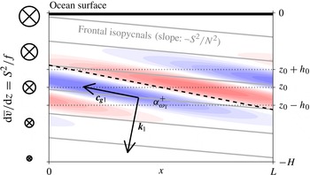
. The forcing is also designed to minimize the generation of potential vorticity, which would modify the mean flow and/or lead to flow instabilities. We systematically check that no negative potential vorticity is generated within the wave maker. The elements of our numerical simulations discussed so far are summarized in figure 4.
Main features of our numerical set-up: frontal isopycnals (grey) and thermal wind
 $\overline{v}$
(left column), domain boundaries and wave maker. The wave maker is centred around
 $z_{0}$
and extends over a distance
 $h_{0}$
around it (dotted horizontal lines). It oscillates in time and space with an intensity proportional to a windowed internal wavefield represented by coloured shades (field and colour axis range arbitrary) of frequency
 ${\it\omega}_{1}$
, wavevector
 $\boldsymbol{k}_{1}$
, group velocity
 $\boldsymbol{c}_{g1}$
, directed along the steep characteristic
 ${\it\alpha}_{{\it\omega}_{1}}^{+}$
(dashed line).

Finally,
 $G(z)\hat{\boldsymbol{y}}$
is a term implemented in order for the upper boundary condition (3.1b
) to be approximately satisfied. Indeed, as explained in Winters et al. (Reference Winters, MacKinnon and Mills2004), our numerical code projects the horizontal momentum equation onto a set of cosine functions, whose vertical derivatives vanish at
 $z=0$
and
 $z=-H$
. In order to satisfy (3.1b
), we follow a procedure inspired by Winters & de la Fuente (Reference Winters and de la Fuente2012), namely to exchange the boundary stress for an interior stress generated by imposing a forcing term in the interior of the fluid that is confined to the vicinity of the boundary over a distance
 ${\it\delta}$
. For the upper boundary, we choose
 $$\begin{eqnarray}G(z)=G_{0}\exp (-(z/{\it\delta})^{2}),\end{eqnarray}$$
with
 ${\it\delta}=3{\rm\Delta}z/4$
.
 $G_{0}$
is determined by constraining
 $\int G\text{d}z$
to match
 ${\it\nu}^{z}\overline{v}_{z}|_{z=0}$
, the desired momentum flux through the upper boundary of the domain:
 $$\begin{eqnarray}\int _{-\infty }^{0}G(z^{\prime })\text{d}z^{\prime }={\it\nu}^{z}\partial _{z}v|_{z=0}={\it\nu}^{z}S^{2}/f,\end{eqnarray}$$
where
 $-\infty$
has been substituted for
 $-H$
, which captures this integral well because
 $H\gg {\it\delta}$
. This yields
 $G_{0}=-2{\it\nu}^{z}S^{2}/(\sqrt{{\rm\pi}}f{\it\delta})$
. A similar boundary condition is implemented at the bottom of the domain.
We use a two-dimensional grid, with
 $n_{x}=256$
points in the horizontal direction, corresponding to a horizontal resolution of
 ${\rm\Delta}x\approx 1.6~\text{m}$
. Unless otherwise stated, we use a vertical resolution
 ${\rm\Delta}z\approx 9.8\times 10^{-2}~\text{m}$
, corresponding to
 $n_{z}=513$
points for
 $H=50~\text{m}$
and
 $n_{z}=1025$
points when
 $H=100~\text{m}$
. The code uses a third-order Adams–Bashforth time-stepping scheme with a time step of
 ${\rm\Delta}t=5~\text{s}$
. All simulations are integrated for 20 forcing periods.
As explained in Winters et al. (Reference Winters, MacKinnon and Mills2004), the code projects all fields onto a discrete set of complex exponentials in the horizontal direction. In the vertical direction, while
 $u$
and
 $v$
are projected onto a set of cosine functions whose vertical derivatives vanish at the top and bottom of the domain,
 $w$
and
 $b$
are projected onto a set of sine functions, which vanish at the top and bottom of the domain. The dynamic pressure
 $p+E$
, where
 $E=|\boldsymbol{u}|^{2}/2$
is the kinetic energy of the perturbations, is computed by taking the divergence of (3.3a
) and inverting the resulting Poisson equation. Since this inversion is straightforward in spectral space, the dynamic pressure is solved algebraically and substituted into the right-hand-side forcing terms of the momentum equations, as explained by Winters et al. (Reference Winters, MacKinnon and Mills2004).
Finally, we neglect the modification of the wave physics by the horizontal component of the Earth’s rotation vector, which we justify in appendix B. By doing so, and like Whitt & Thomas (Reference Whitt and Thomas2013), we follow the recommendations of Colin de Verdière (Reference Colin de Verdière2012), who determined that in a typical oceanic front, effects associated with the thermal wind shear and vertical stratification overwhelm non-traditional effects.
4. Linear numerical simulations
In order to illustrate the basic concepts of critical and near-critical reflections in the context of oceanic fronts, we set all explicit advection operators to zero
 $(\boldsymbol{u}\boldsymbol{\cdot }\boldsymbol{{\rm\nabla}}\equiv ~0)$
, preventing all nonlinear interactions between perturbation modes but retaining their interactions with the stratification and the thermal wind.
4.1. Critical reflection
 $({\it\omega}=f)$

We define a non-dimensional measure of the frequency,
 ${\it\gamma}$
, such that
 $$\begin{eqnarray}{\it\omega}_{1}={\it\omega}_{m}+(\,f-{\it\omega}_{m}){\it\gamma},\end{eqnarray}$$
where
 ${\it\omega}_{1}={\it\omega}_{m}$
when
 ${\it\gamma}=0$
and
 ${\it\omega}=f$
when
 ${\it\gamma}=1$
. We also set
 ${\it\nu}^{z}=2\times 10^{-6}~\text{m}^{2}~\text{s}^{-1}$
,
 ${\it\nu}_{4}^{h}=0.5~\text{m}^{4}~\text{s}^{-1}$
and
 $H=50~\text{m}$
. The amplitude of the forcing,
 $A$
(cf. (3.4) and the definition of
 ${\it\Phi}$
), is set to
 $3.2\times 10^{-8}~\text{m}~\text{s}^{-2}$
, which yields a wave velocity of amplitude
 $U_{1}\approx 1~\text{mm}~\text{s}^{-1}$
, that corresponds to an ‘along-
 $x$
Richardson number’
 $\mathit{Ri}_{1}=(N/mU_{1})^{2}$
of approximately 10.
Throughout the rest of the article, we use complex demodulation (CD) filtering to study the spatial structure of the spectral content at a given frequency of the solution and its decomposition into upward- and downward-propagating signals. The CD filtering is accomplished using the method of Mercier, Garnier & Dauxois (Reference Mercier, Garnier and Dauxois2008) adapted for our application (see appendix C for details). We denote the spectral content of, say,
 $u$
at frequency
 ${\it\omega}$
as
 $U_{{\it\omega}}$
, and its upward- and downward-propagating signals as
 $U_{{\it\omega}}^{u}$
and
 $U_{{\it\omega}}^{d}$
, respectively. Here and throughout the rest of the article, we filter our fields over the last ten forcing periods of the simulations, during which the flow is in a state of forced–dissipative balance and oscillations are steady in amplitude. Note that these CD-filtered fields are complex: for example,
 $\text{Re}[U_{{\it\omega}}]$
, where
 $\text{Re}$
denotes the real part, is the reconstruction of the
 ${\it\omega}$
-oscillating signal at a given phase and its modulus
 $|U_{{\it\omega}}|$
is its amplitude.
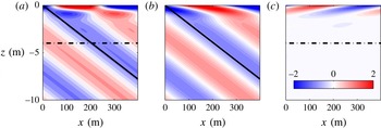
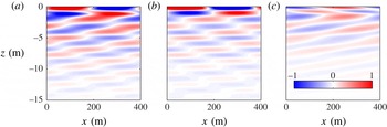
These quantities are shown in figure 5 for the case of critical reflection (
 ${\it\gamma}=1$
,
 ${\it\omega}=f$
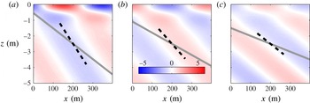
). As expected, no wave propagates back downwards after reflection from the ocean surface, except for a signal in the top 1 to 2 m of the domain and whose scale is set by viscous effects (Grisouard & Thomas, in preparation). Upon reflection, the amplitude of the wave is intensified in a boundary layer near the surface. The strength of this intensification depends on the slope of the isopycnals of the background flow since this slope sets the angle of the steep characteristics of inertial waves (figure 6). Consequently, the stronger the front (as measured by the isopycnal slope and Richardson number of the background flow), the greater the compression of ray tubes during critical reflection, and thus the greater the amplification of the waves.
The velocity in the
 $x$
direction,
 $u$
, in
 $\text{mm}~\text{s}^{-1}$
, CD-filtered to isolate the signal at
 ${\it\omega}=f$
, for a linear simulation and critical reflection (
 ${\it\gamma}=1$
). The full signal at
 ${\it\omega}=f$
,
 $\text{Re}[U_{f}]$
(a), and its upward,
 $\text{Re}[U_{f}^{u}]$
(b) and downward
 $\text{Re}[U_{f}^{d}]$
(c) propagating components. Solid lines indicate the steep characteristic slope, dash-dotted lines the shallow one.

Snapshots of the along-
 $x$
velocity
 $u$
, each normalized by its peak value at
 $z=-2$
m for three linear simulations with
 ${\it\gamma}=1$
(critical reflection) and
 ${\it\nu}^{z}=2\times 10^{-6}~\text{m}^{2}~\text{s}^{-1}$
, for different values of
 $\overline{\mathit{Ri}}$
: 1.05 (a), 2 (b) and 4 (c). The grey lines mark the inclination of undisturbed isopycnals and the dashed lines the inclination of the steep characteristic. The colour scale is the same throughout the panels.

4.2. Forward reflection (
${\it\omega}>f$
)

We now turn to the forward reflection case, and run a simulation, identical to the one described in § 4.1, except
 ${\it\gamma}=2~({\it\omega}_{1}\approx 1.8\times f)$
and
 $A=6.9\times 10^{-8}~\text{m}~\text{s}^{-2}~(\mathit{Ri}_{1}\approx 10)$
. We present the CD-filtered fields for
 $u$
in figure 7.
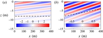
Same as figure 5, but for
 ${\it\gamma}=2$
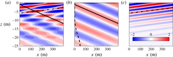
(forward reflection), CD-filtered at the forcing frequency. Note that the vertical axis range is different, and that a dashed line in (b) indicates
 ${\it\Phi}_{0}$
, the position and relative amplitude of the wave maker.

The full filtered signal at
 ${\it\omega}={\it\omega}_{1}$
displayed in figure 7(a) shows an interference pattern, corresponding to a superposition of an upward-propagating wave (figure 7
b), which is radiated from the wave maker, and a downward-propagating wave (figure 7
c), reflected from the surface and with phase lines that align with the predicted angle of the shallow characteristic.
The reflected component decays with depth. This can be understood in terms of viscous damping. Indeed, consider a wavepacket of vertical wavevector
 $\boldsymbol{m}$
whose energy propagates in the direction of its group velocity
 $\boldsymbol{c}_{g}$
. Neglecting horizontal dissipative processes, the amplitude of the wavepacket decays with an e-folding time scale of
 $({\it\nu}^{z}m^{2})^{-1}$
, or with an e-folding vertical length scale of
 $|c_{g}^{z}|({\it\nu}^{z}m^{2})^{-1}$
. In our case, wavepackets originate from the reflection of the incident wave from the surface. Their wavenumber is
 $m_{r}=-k_{1}/{\it\alpha}_{{\it\omega}_{1}}^{-}$
, and
 $|c_{g}^{z}|({\it\nu}^{z}m_{r}^{2})^{-1}\approx 5.0~\text{m}$
. A linear regression of
 $\ln \langle |U_{{\it\omega}_{1}}^{d}|\rangle$
over the top 20 m of the domain, where
 $\langle \cdot \rangle$
denotes the horizontal, along-
 $x$
average, yields the vertical decay length scale of the reflected wave, namely 5.5 m, in good agreement with the predicted value.
4.3. Backward reflection (
${\it\omega}<f$
)

We now run a simulation, similar to the ones described in §§ 4.1 and 4.2, except for
 ${\it\gamma}=0.3$
(
 ${\it\omega}_{1}\approx 0.45\times f$
),
 $A=2.4\times 10^{-8}~\text{m}~\text{s}^{-2}~(\mathit{Ri}_{1}\approx 10)$
,
 $n_{z}=1025$
(
 ${\rm\Delta}z\approx 4.88~\text{cm}$
) and
 ${\it\nu}^{z}=5\times 10^{-7}~\text{m}^{2}~\text{s}^{-1}$
. The increased vertical resolution and decreased vertical viscosity serve two purposes. First, they allow the reflected wave to propagate over a few vertical wavelengths before being completely dissipated. Second, strong viscous effects induce strong distortions in the propagation properties of NIWs, especially for backward-reflected waves. Addressing these distortions is outside the scope of the present article, and is discussed in a companion article (Grisouard & Thomas, in preparation). We present CD-filtered fields for
 $u$
in figure 8.
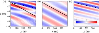
Same as figure 7 but for
 ${\it\gamma}=0.3$
(backward reflection) and
 ${\it\nu}^{z}=5\times 10^{-7}~\text{m}^{2}~\text{s}^{-1}$
.

Similarly to the forward-reflection case, incident and reflected waves propagate along the steep and shallow characteristics, except that now the shallow characteristic corresponds to backward-propagating waves (cf. figure 8). We have
 $|c_{g}^{z}|({\it\nu}^{z}m_{r}^{2})^{-1}\approx 5.1~\text{m}$
for the linearly predicted decay scale, which compares well with our numerical simulation, where we estimate an e-folding decay scale of 5.3 m.
Note that if the viscosity had been kept at the initial value, namely
 ${\it\nu}^{z}=2\times 10^{-6}~\text{m}^{2}~\text{s}^{-1}$
, backward-reflected waves would have propagated less far vertically than their forward-reflected counterparts. As will be described in the next section, nonlinear effects reinforce this tendency of forward reflections to be associated with stronger downward energy propagation.
5. Nonlinear numerical simulations of near-critical reflections
5.1. On the asymmetry between forward and backward nonlinear reflections
In the classical case of waves reflecting off slopes, other authors (Peacock & Tabaei Reference Peacock and Tabaei2005; Tabaei, Akylas & Lamb Reference Tabaei, Akylas and Lamb2005) have observed that the generation of super-harmonics, namely waves of frequencies that are multiples of the forcing frequency, is often observed during forward reflections, but is hardly detectable in the case of backward reflections.
In forward reflections, how the group speeds of these nonlinearly generated higher-frequency waves compare with that of the linearly reflected wave is the result of a competition between (i) their higher wavenumbers (Thorpe & Haines Reference Thorpe and Haines1987; Gostiaux et al. Reference Gostiaux, Dauxois, Didelle, Sommeria and Viboud2006), which slows them down (cf. (2.12)), and (ii) their propagation along steeper characteristics, which increases their vertical group velocity. In our parameter regime, the result of this competition is that higher-frequency energy propagation is vertically faster and further reaching than for the linearly reflected waves.
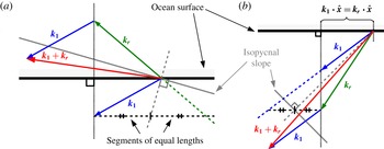
Typical wavevector configurations for forward (a) and backward (b) reflections under the hydrostatic approximation. The main features of linear reflections are highlighted. Firstly, the incident and reflected characteristics (not displayed) have slopes symmetric with respect to the isopycnal slope. The wavevectors of the incident and reflected waves,
 $\boldsymbol{k}_{1}$
and
 $\boldsymbol{k}_{r}$
, respectively, are perpendicular to their characteristics. Secondly, the horizontal components of
 $\boldsymbol{k}_{1}$
and
 $\boldsymbol{k}_{r}$
are equal. In the forward reflection case (a), the forced wavevector
 $\boldsymbol{k}_{1}+\boldsymbol{k}_{r}$
runs more parallel to isopycnals compared to
 $\boldsymbol{k}_{1}$
or
 $\boldsymbol{k}_{r}$
, similar to freely propagating waves of higher frequency. In backward reflections (b),
 $\boldsymbol{k}_{1}+\boldsymbol{k}_{r}$
runs more perpendicular to isopycnals than either
 $\boldsymbol{k}_{1}$
or
 $\boldsymbol{k}_{r}$
, which for a higher-frequency oscillation is not consistent with the dispersion relation.

On the other hand, backward reflections tend to be associated with much weaker super-harmonic generation. Jiang & Marcus (Reference Jiang and Marcus2009) have provided theoretical arguments to explain this asymmetry between backward and forward reflections, which we summarize here. The nonlinear interaction of two plane internal waves characterized by frequencies and wavevectors
 $({\it\omega}^{\prime },\boldsymbol{k}^{\prime })$
and
 $({\it\omega}^{\prime \prime },\boldsymbol{k}^{\prime \prime })$
generates a third oscillation characterized by
 $({\it\omega}^{\prime }+{\it\omega}^{\prime \prime },\boldsymbol{k}^{\prime }+\boldsymbol{k}^{\prime \prime })$
. When
 ${\it\omega}^{\prime }+{\it\omega}^{\prime \prime }$
and
 $\boldsymbol{k}^{\prime }+\boldsymbol{k}^{\prime \prime }$
satisfy the dispersion relation, the triad is resonant and the energy transfer towards the
 $({\it\omega}^{\prime }+{\it\omega}^{\prime \prime })$
-frequency wave is efficient. In general, the closer the third oscillation is to a resonant configuration, the stronger the generation of the super-harmonic wave. In the case of wave reflection on a slope, the two interacting waves are the incident and the reflected waves and
 ${\it\omega}^{\prime }$
and
 ${\it\omega}^{\prime \prime }$
are identical. For a given slope angle, and provided that this slope does not exceed a certain value, two incident wave frequencies satisfy this resonance condition (Thorpe & Haines Reference Thorpe and Haines1987), both of which corresponding to forward reflections. (Note that if instead of a plane wave, the incident wave is in the form of a beam, these considerations about resonance probably do not apply (Tabaei et al.
Reference Tabaei, Akylas and Lamb2005; Rodenborn et al.
Reference Rodenborn, Kiefer, Zhang and Swinney2011).) On the other hand, as shown by Jiang & Marcus (Reference Jiang and Marcus2009), resonance cannot occur in the backward-reflecting range.
The same reasoning can easily be applied to our frontal case and is sketched in figure 9. We recall from § 2.3 that the linear reflection of plane internal waves from a horizontal boundary is constrained by the conservation of the horizontal wavenumber
 $k_{1}$
as well as the dispersion relation of internal waves (2.6). Let us then consider an incident wave propagating along the steep characteristic, and a reflected wave propagating along the shallow characteristic. Their nonlinear interaction will force a third wave whose wavevector is the sum of those of the interacting waves. As illustrated in figure 9, the wavevector of the forced wave in backward reflection runs more perpendicular to isopycnals, which if resonant, would be associated with a wave frequency closer to the minimum frequency (cf. (2.7)) than the frequency of the incident and reflected waves. Hence backward reflections cannot generate freely propagating super-harmonics through triad resonant interactions. For forward reflections, in contrast, the forced wavevector can run more parallel to isopycnals, consistent with a wave of higher frequency, thus making it possible for the creation of super-harmonics through triad resonant interactions.
5.2. Forward reflection (
${\it\omega}_{1}>f$
)

We now run a simulation, similar to the one described in § 4.2, except that it is now fully nonlinear. As before,
 ${\it\gamma}=2~({\it\omega}_{1}\approx 1.8\times f)$
,
 ${\it\nu}^{z}=2\times 10^{-6}~\text{m}^{2}~\text{s}^{-1}$
and
 $\mathit{Ri}_{1}\approx 10$
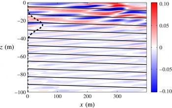
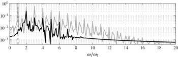
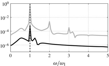
. As expected from the arguments described in § 5.1, a snapshot of the vertical velocity (figure 10) reveals that energy is able to propagate downwards over the whole water column. Moreover, figure 11 shows that while the frequency spectrum above the forcing region exhibits the forcing frequency as the dominant frequency, only higher harmonics are visible below the forcing region. Indeed, once a strong
 $2{\it\omega}_{1}$
-frequency wave is generated, the number of possible interactions grows, i.e.
 ${\it\omega}_{1}$
and
 $2{\it\omega}_{1}$
oscillations can interact to form
 $3{\it\omega}_{1}$
-frequency waves, etc., in a process akin to wave turbulence.
Snapshot of
 $w~(\text{mm}~\text{s}^{-1})$
in a fully nonlinear simulation for
 ${\it\gamma}=2$
(forward reflection),
 ${\it\nu}^{z}=2\times 10^{-6}~\text{m}^{2}~\text{s}^{-1}$
and
 $\mathit{Ri}_{1}\approx 10$
. Isopycnals of the full flow are contoured in black and the dashed line identifies
 ${\it\Phi}_{0}$
.

Frequency spectra of
 $w$
for a nonlinear simulation with
 ${\it\gamma}=2$
(forward reflection),
 ${\it\nu}^{z}=2\times 10^{-6}~\text{m}^{2}~\text{s}^{-1}$
and
 $\mathit{Ri}_{1}\approx 10$
. The spectra are evaluated at depths
 $z=-10~\text{m}$
(grey) and
 $z=-50~\text{m}$
(black), averaged along
 $x$
and normalized by the maximum value at
 $z=-10~\text{m}$
. The dashed vertical line marks
 ${\it\omega}={\it\omega}_{1}$
.

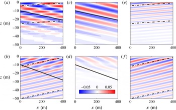
We use CD filtering to isolate the spatial structure of oscillations at the forcing frequency and its harmonics (figure 12). For the former, phase lines and the theoretical predictions for the characteristics align well (cf. figure 12
c,e), similar to the linear simulations. For the signal at
 $2{\it\omega}_{1}$
however, we find a misalignment between phase lines and characteristics in the top 30 m of the domain (cf. figure 12
f). This was to be expected, based on the arguments described in § 5.1, since we have not tuned
 ${\it\omega}_{1}$
to excite a resonance. We can evaluate the degree of resonance by calculating the quantity
 $(m_{1}+m_{r})/m_{2}$
, where
 $m_{1}$
and
 $m_{r}$
are the vertical wavenumbers of the incident and reflected waves and
 $m_{2}$
is the vertical wavenumber of the second harmonic calculated using the dispersion relation (2.6) and assuming
 $k=2k_{1}$
. This parameter is equal to unity at resonance; however for this simulation it is close to 0.5, indicating that the flow is only near resonance. Therefore, the phase lines of the forced waves are not expected to align with the characteristics of freely propagating waves. Below a certain depth however, free downward-propagating harmonics are observed. For example, below
 $z=-30~\text{m}$
in figure 12(f), we can observe a field of
 $2{\it\omega}_{1}$
-frequency waves ‘escaping’ the region where waves are generated.
CD-filtered vertical velocity in a fully nonlinear simulation with
 ${\it\gamma}=2$
(forward reflection),
 $\mathit{Ri}_{1}\approx 10$
and
 ${\it\nu}^{z}=2\times 10^{-6}~\text{m}^{2}~\text{s}^{-1}$
. Panels (a,c,e) and (b,d,f) correspond to
 $W_{{\it\omega}_{1}}$
and
 $W_{2{\it\omega}_{1}}$
, respectively; (a,b) contain both upward and downward components, while (c,d) and (e,f) are the upward and downward components, respectively: (a)
 $\text{Re}[W_{{\it\omega}1}]$
; (b)
 $\text{Re}[W_{2{\it\omega}1}]$
; (c)
 $\text{Re}[W_{{\it\omega}1}^{u}]$
; (d)
 $\text{Re}[W_{2{\it\omega}1}^{u}]$
; (e)
 $\text{Re}[W_{{\it\omega}1}^{d}]$
; ( f)
 $\text{Re}[W_{2{\it\omega}1}^{d}]$
. The colour scale is in
 $\text{mm}~\text{s}^{-1}$
and applies to all panels. Solid lines indicates the steep characteristic slope, dash-dotted lines the shallow one.

5.3. Backward reflection (
${\it\omega}_{1}<f$
)

We now run a simulation, similar to the one described in § 4.3, although fully nonlinear. As before,
 ${\it\gamma}=0.3~({\it\omega}_{1}\approx 0.45\times f)$
,
 ${\it\nu}^{z}=5\times 10^{-7}~\text{m}^{2}~\text{s}^{-1}$
and
 $\mathit{Ri}_{1}\approx 10$
.
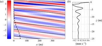
As expected from our conclusions in § 5.1, the reflection does not induce freely propagating higher harmonics, as a revealed by a snapshot of
 $u$
(figure 13
a), as well as frequency spectra above and below the forcing region (figure 14). In the latter figure, the dominant peaks are the forcing frequency, and the higher harmonics visible on figure 11 have virtually disappeared. Note that the peak at the forcing frequency is visible below the forcing region, contrary to the forward reflection shown in figure 11. A careful comparison reveals that the relative amplitude of this peak is actually smaller for the backward reflection (figure 14) than for the forward reflection (figure 11), which is indicative of a nearly complete absence of higher harmonics in the backward reflection rather than a stronger linear reflection.
Snapshots of (a)
 $u~(\text{mm}~\text{s}^{-1})$
and (b) its lateral average,
 $\langle u\rangle ~(\text{mm}~\text{s}^{-1})$
, in a fully nonlinear simulation for
 ${\it\gamma}=0.3$
(backward reflection),
 $\mathit{Ri}_{1}\approx 10$
and
 ${\it\nu}^{z}=5\times 10^{-7}~\text{m}^{2}~\text{s}^{-1}$
. Isopycnals are contoured in black in (a), and the dashed line shows the location of the forcing envelope
 ${\it\Phi}_{0}$
.

Same as figure 11 but for
 ${\it\gamma}=0.3$
(backward reflection), and where the black line is now the spectrum evaluated at
 $z=-45~\text{m}$
.

Nonlinear effects are present however, as revealed by the presence of a non-zero laterally mean flow
 $\langle u\rangle$
(cf. figure 13
b). The horizontal mean flow exhibits a vertical wavelength of 4.2 m, estimated from the average peak-to-peak distance. This flow is approximately stationary in time and, indeed, its vertical wavelength is comparable to the vertical wavelength of a zero-frequency wave generated by a nonlinear interaction of incident and reflected waves in which frequencies are subtracted, i.e.
 $\ell =2{\rm\pi}/|m_{1}-m_{r}|=4.0~\text{m}$
, where
 $m_{1}=-k_{1}/{\it\alpha}_{{\it\omega}_{1}}^{+}$
and
 $m_{r}=-k_{1}/{\it\alpha}_{{\it\omega}_{1}}^{-}$
. This interaction is non-resonant, as are the interactions potentially generating super-harmonics and therefore no propagating wave of higher frequency is generated, and all motion is confined to regions where incident and reflected waves overlap. Note that this mean flow is purely horizontal, and therefore does not appear in the spectra of
 $w$
shown in figure 14.
6. Nonlinear numerical simulation of a critical reflection
$({\it\omega}_{1}=f)$

As we saw in the previous section, forward reflections of super-inertial waves induce deep energy propagation, while backward reflections of sub-inertial waves do not. We now focus on the intermediate case, namely the critical reflection of inertial waves.
6.1. Overall behaviour
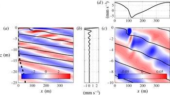
To begin with, we run the fully nonlinear version of the linear experiment described in § 4.1. Snapshots of the velocity field are shown in figure 15. Strikingly, the effect of the reflection is felt over a larger depth than in the linear case presented in § 4.1. Indeed, the incoming wave is perturbed over a depth of around 10 m (to be compared with e.g. the viscous oscillating boundary layer thickness
 $\sqrt{{\it\nu}^{z}/f}\approx 14~\text{cm}$
, or the metre-thick boundary layer observed in the linear case, § 4.1). This simulation also has a horizontally averaged flow
 $\langle u\rangle$
that oscillates in the vertical with a wavelength of approximately 2 m and decays with depth in a quasi-exponential manner (figure 15
b). Similar to the nonlinear simulation of backward reflection presented in § 5.3, this laterally averaged flow is also approximately stationary in time, suggesting that this flow is the result of non-resonant, nonlinear interactions. We will elaborate on this point in the rest of this section.
Snapshots of the fully nonlinear velocity fields for
 ${\it\gamma}=1$
(critical reflection),
 ${\it\nu}^{z}=2\times 10^{-6}~\text{m}^{2}~\text{s}^{-1}$
and
 $\mathit{Ri}_{1}\approx 10$
. (a) Colour:
 $u~(\text{mm}~\text{s}^{-1})$
; solid lines: isopycnals; dashed line:
 ${\it\Phi}_{0}$
. (b) Snapshot of
 $\langle u\rangle ~(\text{mm}~\text{s}^{-1})$
. (c) Colour:
 $w~(\text{mm}~\text{s}^{-1})$
; solid lines: same as for (a). (d)
 $u|_{z=0}~(\text{mm}~\text{s}^{-1})$
.

Note that in the classical case, Thorpe & Haines (Reference Thorpe and Haines1987) predict the existence of a time-mean flow, flowing parallel to the boundary when waves reflect off it (cf. also Grisouard et al. Reference Grisouard, Leclair, Gostiaux and Staquet2013; Zhou & Diamessis Reference Zhou and Diamessis2013). However, this flow appears only in off-critical reflection cases.
Another feature of nonlinear, critical reflections are bores. For example, in the snapshots of
 $w$
and
 $u|_{z=0}$
, shown in figures 15(c) and 15(d), respectively, a bore is located around
 $x=110~\text{m}$
that induces sharp lateral variations in
 $u$
, and extends downwards in the form of alternating vertical velocity perturbations that decay with depth. The bore is approximately 20 m wide, a width that does not seem to depend on the horizontal biharmonic dissipation, as a simulation with
 ${\it\nu}_{4}^{h}=10~\text{m}^{4}~\text{s}^{-1}$
(a twenty-fold increase of
 ${\it\nu}_{4}^{h}$
, not shown) suggests. Bores have been observed in classical critical reflections from an inclined slope by Cacchione & Wunsch (Reference Cacchione and Wunsch1974) and are predicted by theory to be ubiquitous (Dauxois & Young Reference Dauxois and Young1999; Thorpe Reference Thorpe1992, Reference Thorpe1999). To our knowledge, they have never been reported in numerical experiments on critical reflections. Our simulation highlights the peculiar vertical structure of the bore, namely the alternating vertical velocity perturbation, which to our knowledge has not been observed nor predicted in the context of classical reflections.
6.2. Harmonics
Critical reflection induces a flow response that extends deep into the water column, although this flow response is very different from that in forward reflection, because no freely propagating higher-frequency wave is generated, as described below. In this sense, critical reflection is closer to backward reflection.
Frequency spectra calculated anywhere in the top 10 m of the domain consist of a series of well-isolated peaks at frequencies that are multiples of
 ${\it\omega}_{1}=f$
. Figure 16 shows the downward-propagating components of the dominant harmonics, at
 $f$
and
 $2f$
. If these harmonics were freely propagating, their phase lines would align with the shallow characteristics, but that is not the case. The characteristics shown in figure 16 were calculated using the properties of the mean flow at
 $t=0$
. Although these properties change with time, the effect on the slope of characteristics is minimal and cannot explain this misalignment with phase lines. Therefore, we can conclude that these motions are forced locally through nonlinear interactions.
CD-filtered
 $u$
, in
 $\text{mm}~\text{s}^{-1}$
, for a fully nonlinear simulation, for
 ${\it\gamma}=1$
(critical reflection),
 ${\it\nu}^{z}=2\times 10^{-6}~\text{m}^{2}~\text{s}^{-1}$
and
 $\mathit{Ri}_{1}\approx 10$
, highlighting the downward-propagating signals at
 $f$
(a,
 $\text{Re}[U_{f}^{d}]$
) and
 $2f$
(b,
 $\text{Re}[U_{2f}^{d}]$
). In both cases, a downward-propagating wave at the filtering frequency would propagate along the shallow characteristics (dash-dotted lines) if it were freely propagating.

Perhaps more surprising is that in principle, and unlike in the forward reflection presented in § 5.2, there could be
 $2f$
-frequency waves, which could freely propagate down along inclined characteristics, say below the region where nonlinear interactions act to force a
 $2f$
-frequency oscillation. This has been observed in the classical case, for example by Gostiaux et al. (Reference Gostiaux, Dauxois, Didelle, Sommeria and Viboud2006) or Gayen & Sarkar (Reference Gayen and Sarkar2010). In our case however, no such radiation of higher harmonics is observed. This is perhaps due to the presence of turbulence in the aforementioned references, while our simulations are only weakly nonlinear.
Each harmonic’s existence is intricately tied to the existence of the others, as a refined analysis of their dynamics show. As we mentioned earlier, the whole flow can be approximated as a sum of harmonics, which are well isolated in frequency. For example,
 $$\begin{eqnarray}u(x,z,t)\approx \mathop{\sum }_{n=-\infty }^{\infty }U_{nf}(x,z)\exp (\text{i}n\,f\,t),\end{eqnarray}$$
where the condition that
 $u$
is real imposes that the complex conjugate of
 $U_{nf}$
be equal to
 $U_{-nf}$
. One can then replace
 $u$
by the above expression in equation [(3.3a
)
 $\,\boldsymbol{\cdot }\hat{\boldsymbol{x}}$
] and project on the relevant complex exponential (cf. (C 1)) so as to isolate the
 $n$
th complex Fourier coefficient. The nonlinear terms, which force the
 $n$
th harmonic, are then
 $$\begin{eqnarray}\frac{1}{T}\int _{t_{0}}^{t_{0}+T}(uu_{x}+wu_{z})\exp (-\text{i}n\,f\,t)\text{d}t=\mathop{\sum }_{j=-\infty }^{\infty }U_{jf}\partial _{x}U_{(n-j)f}+W_{jf}\partial _{z}U_{(n-j)f}.\end{eqnarray}$$
For our calculations,
 $t_{0}=T=20{\rm\pi}/f$
. The equation above highlights the fact that for a given frequency
 $n\,f$
, the nonlinearly forced motion is the result of an infinite number of triadic interactions between waves whose frequencies add up to
 $n\,f$
. Because all our fields are real, we can re-write (6.2) as
 $$\begin{eqnarray}{\it\Lambda}_{nf}=\mathop{\sum }_{j=0}^{\infty }{\it\Lambda}_{nf}^{(\,j)},\quad \text{where}~{\it\Lambda}_{nf}=\frac{1}{T}\int _{t_{0}}^{t_{0}+T}(uu_{x}+wu_{z})\exp (-\text{i}n\,f\,t)\text{d}t\end{eqnarray}$$
and
 $$\begin{eqnarray}{\it\Lambda}_{nf}^{(\,j)}=2\left[U_{If}\partial _{x}U_{Jf}+W_{If}\partial _{z}U_{Jf}+(1-{\it\delta}_{IJ})(U_{Jf}\partial _{x}U_{If}+W_{Jf}\partial _{z}U_{If})\right]\!,\end{eqnarray}$$
where
 $$\begin{eqnarray}I=\lfloor n/2\rfloor -j\quad \text{and}\quad J=\lceil n/2\rceil +j\quad (\text{note that}~I+J=n),\end{eqnarray}$$
in which
 $\lfloor \cdot \rfloor$
and
 $\lceil \cdot \rceil$
are the floor and ceiling operators, respectively, and where the Kronecker delta
 ${\it\delta}_{IJ}$
avoids double counts (note that the sum in (6.2) starts at
 $-\infty$
, while the one in (6.3) starts at 0). The interpretation of (6.3) is that
 ${\it\Lambda}_{nf}$
is the sum of all terms that force an oscillation in real space at a frequency
 $n\,f$
. As for each individual
 ${\it\Lambda}_{nf}^{(\,j)}$
, it collects all terms corresponding to the interaction between waves of frequencies
 $|If|$
and
 $|Jf|$
.
For low values of
 $n$
, only a few
 ${\it\Lambda}_{nf}^{(\,j)}$
are significant. For example, the nonlinear forcing of the
 $f$
-frequency motion (
 $n=1$
), shown in figure 17(a), is well captured by simply adding
 ${\it\Lambda}_{1f}^{(0)}$
and
 ${\it\Lambda}_{1f}^{(1)}$
. That is, the forced motion shown in figure 16(a) is the result of non-resonant triadic interactions between both zero- and
 $f$
-frequency motions (
 ${\it\Lambda}_{1f}^{(0)}$
,
 $I=0$
,
 $J=1$
, cf. figure 17
b) and
 $f$
- and
 $2f$
-frequency oscillations (
 ${\it\Lambda}_{1f}^{(1)}$
,
 $I=-1$
,
 $J=2$
, cf. figure 17
c).
(a)
 ${\it\Lambda}_{1f}$
, (b)
 ${\it\Lambda}_{1f}^{(0)}$
and (c)
 ${\it\Lambda}_{1f}^{(1)}$
for a fully nonlinear simulation, with
 ${\it\gamma}=1$
(critical reflection),
 $\mathit{Ri}_{1}\approx 10$
and
 ${\it\nu}^{z}=2\times 10^{-6}~\text{m}^{2}~\text{s}^{-1}$
; see (6.3) for notation. Units for all panels are
 $10^{-7}~\text{m}~\text{s}^{-2}$
.

The zero- and
 $2f$
-frequency oscillations, which can force oscillations at
 $f$
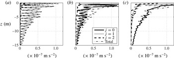
, are themselves the result of non-resonant, triadic interactions. This is illustrated in figure 18, which shows the vertical structure of the lateral average of the magnitude of a few nonlinear forcing terms,
 $\langle |{\it\Lambda}_{nf}|\rangle$
, and of their constituents,
 $\langle |{\it\Lambda}_{nf}^{(\,j)}|\rangle$
. For example, the mean flow is driven almost exclusively by
 ${\it\Lambda}_{0f}^{(1)}~(I=-1,J=1)$
, the interaction between upward- and downward-propagating oscillations at frequency
 $f$
(see figure 18
a). For the second harmonic, figure 18(c) shows that once again, interactions between
 $f$
-frequency oscillations capture the main forcing pattern, since
 ${\it\Lambda}_{2f}^{(0)}~(I=J=1)$
is the dominant term. In contrast, the nonlinear driving term for inertial motions,
 ${\it\Lambda}_{1f}$
, involves interactions between the first harmonic and both the mean flow and second harmonic via
 ${\it\Lambda}_{1f}^{(0)}$
and
 ${\it\Lambda}_{1f}^{(1)}$
(figure 18
b).
Laterally averaged nonlinear forcing terms
 $\langle |{\it\Lambda}_{nf}^{(\,j)}|\rangle$
for the mean flow (
 $n=0$
)
 $\langle |{\it\Lambda}_{0f}^{(\,j)}|\rangle$
(a), inertial motions (
 $n=1$
)
 $\langle |{\it\Lambda}_{1f}^{(\,j)}|\rangle$
(b) and the second harmonic (
 $n=2$
)
 $\langle |{\it\Lambda}_{2f}^{(\,j)}|\rangle$
(c). ‘Total’ refers to
 $\langle |{\it\Lambda}_{nf}|\rangle$
.

Figure 18 highlights how the vertical extent of oscillating motion of critical reflection in this system is the result of the mutual interaction of non-resonantly forced harmonics. In this way, energy can penetrate well into the interior. That is not to say that dissipation is unimportant in this system. Indeed, we will see next that viscosity is the main agent of the decay of the nonlinear flow with depth.
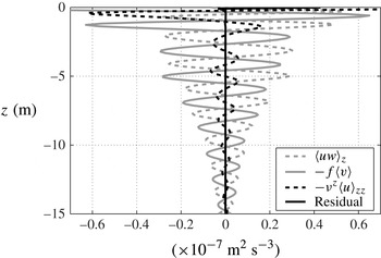
6.3. Horizontally averaged flow
We now use the horizontally averaged flow as a proxy to retrieve more information about the harmonics. Indeed, as we just saw, the harmonics form a network of interacting triads, and are all closely tied to each other. Therefore, studying one harmonic in particular gives some information about the spatial structure of the rest. We choose the zero-frequency component because it has the simplest spatial structure. Indeed, the time-mean flow is mostly the result of interactions between two inertial oscillations whose frequencies cancel, as for the backward reflection in § 5.3. This also implies that the horizontal wavenumber of the former is the difference between the horizontal wavenumbers of the latter, namely zero. Because the laterally averaged flow is also stationary in time, as mentioned in § 6.1, we can conclude that the lateral and time averages are virtually identical. We therefore study the
 $x$
-averaged flow, and in particular the
 $x$
-momentum equation, taking into account the fact that
 $\partial _{t}\langle u\rangle \approx 0$
:
 $$\begin{eqnarray}\left\langle uw\right\rangle _{z}-f\left\langle v\right\rangle -{\it\nu}^{z}\left\langle u\right\rangle _{zz}=0.\end{eqnarray}$$
Figure 19 displays the three terms of (6.6) and shows that each of them plays a non-negligible role in achieving the balance. In other words, the sub-surface flow is achieved by a balance between vertical advection, friction and the Coriolis acceleration.
Terms, constitutive of (6.6), the
 $x$
-averaged, along-
 $x$
momentum equation in a fully nonlinear simulation, with
 ${\it\gamma}=1$
(critical reflection),
 ${\it\nu}^{z}=2\times 10^{-6}~\text{m}^{2}~\text{s}^{-1}$
and
 $\mathit{Ri}_{1}\approx 10$
.

As a consequence, the spatial structure of the zero-frequency harmonic is dependent on
 ${\it\nu}^{z}$
and the forcing amplitude. We check this with additional numerical simulations, with a new set of parameters including
 $\mathit{Ri}_{1}\approx 100$
(up from 10) and
 ${\it\nu}^{z}=4\times 10^{-6}~\text{m}^{2}~\text{s}^{-1}$
(increased from
 $2\times 10^{-6}~\text{m}^{2}~\text{s}^{-1}$
). For each numerical experiment, the profile of
 $\langle u\rangle$
(such as the one presented in figure 15
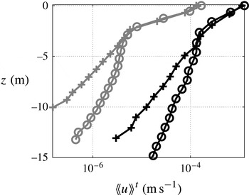
b) is averaged in time over the last ten forcing periods of the simulations, which removes small residual fluctuations in time. The depth and amplitude of each local peak of
 $\langle \!\langle u\rangle \!\rangle ^{t}$
, where
 $\langle \cdot \rangle ^{t}$
is the time average operator, is then measured, from which we retrieve the envelope of the vertical oscillations in
 $\langle \!\langle u\rangle \!\rangle ^{t}$
(see figure 20). A semi-logarithmic scale highlights the spatial range(s) over which the envelope decays exponentially with depth. All numerical experiments exhibit a sharp exponential decay of the envelope with depth immediately under the surface, until approximately
 $z=-2.5~\text{m}$
. The decay is more pronounced for weaker amplitude, but does not seem to depend on the viscosity. Below
 $z=-2.5~\text{m}$
, the decay is more moderate, and the reverse happens: the decay length scale depends on viscosity, but not on the forcing amplitude. Simulations run with different biharmonic viscosities,
 ${\it\nu}_{4}^{h}$
, exhibit essentially the same behaviour, implying that horizontal dissipation plays a negligible role in the dynamics.
Amplitudes of the local maxima as a function of depth of
 $\langle \!\langle u\rangle \!\rangle ^{t}$
in
 $\text{m}~\text{s}^{-1}$
in a fully nonlinear simulation with
 ${\it\gamma}=1$
(critical reflection). Black symbols are for
 $\mathit{Ri}_{1}\approx 10$
and grey symbols are for
 $\mathit{Ri}_{1}\approx 100$
; circles are for
 ${\it\nu}^{z}=2\times 10^{-6}~\text{m}^{2}~\text{s}^{-1}$
, crosses for
 ${\it\nu}^{z}=4\times 10^{-6}~\text{m}^{2}~\text{s}^{-1}$
.

For most of the depth over which the harmonics exist, their decay strongly depends on
 ${\it\nu}^{z}$
. This suggests that if the viscosity were reduced, harmonics could extend deeper into the interior. This goes against the classical notion of critical reflection being associated with the absorption of most of the energy in the immediate vicinity of the boundary, as has been documented in the literature (e.g. Cacchione & Wunsch Reference Cacchione and Wunsch1974; Ivey & Nokes Reference Ivey and Nokes1989; Slinn & Riley Reference Slinn and Riley1996; Gostiaux et al.
Reference Gostiaux, Dauxois, Didelle, Sommeria and Viboud2006; Gayen & Sarkar Reference Gayen and Sarkar2010). Note that some of these references describe the radiation of energy into the interior of the fluid via freely propagating harmonics. These waves, generated in the boundary layer and which then propagate freely into the fluid, are very different from the oscillations found in our cluster of forced triads, which are generated throughout the water column, and which cannot propagate freely.
7. Discussion and conclusions
At a front, inertial waves can travel on two distinct characteristics, one flat and one tilted at twice the slope of isopycnals. When inertial waves propagating upward on the steep characteristic collide with the sea surface, and reflect onto the flat characteristic, they can experience amplification following a process akin to critical reflection of classical internal waves from a sloping wall (Phillips Reference Phillips1966) or of non-traditional NIWs from flat surfaces (Gerkema & Shrira Reference Gerkema and Shrira2005). Fully nonlinear numerical simulations highlight the stark asymmetry between forward reflections (
 ${\it\omega}>f$
), for which incident and reflected waves can interact near-resonantly, trigger a wave–turbulence cascade towards higher frequencies and redistribute energy vertically, and backward reflections (
 ${\it\omega}<f$
), for which nonlinear interactions are too off-resonant to generate freely propagating high-frequency waves. In the case of frontal critical reflection (
 ${\it\omega}=f$
), we find that energy extends far below the surface. In contrast to classical critical reflection (Gostiaux et al.
Reference Gostiaux, Dauxois, Didelle, Sommeria and Viboud2006), this energy is not in a freely propagating wave form, but rather exists as a cluster of non-resonant interacting triads. Friction affects the dynamics of these forced oscillations and our numerical simulations show that as viscosity is reduced they penetrate deeper into the ocean interior.
For critical reflection at a front to occur, inertial waves must be generated on the steep characteristic. In our numerical simulations this was accomplished by the wave maker (3.4). One mechanism that could radiate inertial waves upward is the instability of lee waves generated by geostrophic currents flowing over rough topography (Nikurashin & Ferrari Reference Nikurashin and Ferrari2010a ). Nikurashin & Ferrari (Reference Nikurashin and Ferrari2010b ) and Nikurashin, Vallis & Adcroft (Reference Nikurashin, Vallis and Adcroft2012) notice in their numerical simulations of the Antarctic Circumpolar Current that all such inertial waves are dissipated well below the surface. The observations of Waterman, Naveira Garabato & Polzin (Reference Waterman, Naveira Garabato and Polzin2013) and Waterman et al. (Reference Waterman, Polzin, Naveira Garabato, Sheen and Forryan2014) contradict this result and show that a significant fraction of the wavefield is able to propagate higher than predicted, although its fate is unclear. It is possible to imagine that these waves could reach the front-rich surface of the Antarctic Circumpolar Current, and experience critical reflection there.
In the ocean, inertial oscillations are most often set in motion by variable winds. Winds primarily induce horizontal forces, which unlike our wave maker are not optimal for accelerating the slantwise motions of the inertial waves on the steep characteristic. This suggests that wind-driven inertial oscillations should not be very effective at triggering critical reflections. However, there are other ways that inertial motions can be generated at fronts that do not require external forcing, such as geostrophic adjustment (Ou Reference Ou1984; Blumen Reference Blumen2000; Plougonven & Zeitlin Reference Plougonven and Zeitlin2005) or rapid frontogenesis (Shakespeare & Taylor Reference Shakespeare and Taylor2013, Reference Shakespeare and Taylor2014). These processes are associated with slantwise ageostrophic near-inertial motions that could radiate waves better suited for critical reflection. Having said this, at realistic ocean frontal flows with vertical vorticity (in contrast to the idealized fronts studied here), the frequency criteria for critical reflection is broader, suggesting that additional wave generation mechanisms could come into play.
In a unidirectional frontal flow with vertical vorticity,
 $\overline{{\it\zeta}}$
, the minimum frequency of inertia–gravity waves (2.7) becomes
 ${\it\omega}_{m}=f\sqrt{1+\overline{{\it\zeta}}/f-1/\overline{\mathit{Ri}}}$
; however the expression for the slope of characteristics (2.8) remains unchanged (Whitt & Thomas Reference Whitt and Thomas2013). Consequently, critical reflection off the sea surface occurs at the effective inertial frequency
 $f_{eff}=f\sqrt{1+\overline{{\it\zeta}}/f}$
rather than
 $f$
. In frequency space, the oceanic near-inertial peak also tends to be spectrally broader than say the internal tide, and therefore spans a somewhat wide range of frequencies around
 ${\it\omega}=f$
. But because fronts are associated with a continuous range of vertical vorticity, which includes
 $\overline{{\it\zeta}}=0$
, a significant portion of the near-inertial peak can potentially be absorbed by critical reflections at fronts. Regions with cyclonic vorticity where
 $f_{eff}>f$
tend to be correlated with enhanced horizontal density gradients at fronts, a phenomenon that can be attributed to strain-driven frontogenesis and conservation of potential vorticity (Thomas et al.
Reference Thomas, Tandon, Mahadevan, Hecht and Hasumi2008). These are regions where isopycnals are steepest and hence wave amplification via critical reflection would be strongest. It follows that critical reflection should be most pronounced for waves with frequencies
 ${\it\omega}=f_{eff}>f$
. Such super-inertial waves are a common feature of the internal wave continuum in the ocean and thus are likely to be readily available for critical reflection at fronts.
For example, one can think of the mechanism considered by Winters et al. (Reference Winters, Bouruet-Aubertot and Gerkema2011), with the case of
 $\text{M}_{2}$
(semi-diurnal) internal tides propagating poleward on a non-traditional
 ${\it\beta}$
-plane towards the latitude 74.5 (North or South). At these ‘inertial’ latitudes, the
 $\text{M}_{2}$
tidal frequency matches
 $|\,f|$
and due to prominent non-traditional effects in the weakly stratified abyss, the internal tide experiences a critical reflection from the flat bottom. The inertial latitude is different for each tidal frequency, and it is easy to imagine a similar process occurring at fronts located in their vicinity, where internal tides, which also happen to be near-inertial, can propagate upward on the steep characteristic and critically reflect against the ocean surface. This phenomenon, combined with the broadening of the critical frequency criterion when
 $\overline{{\it\zeta}}\neq 0$
, could mean that internal tides could critically reflect against the ocean surface at fronts located in a broad latitudinal range around their inertial latitude.
Unlike classical or non-traditional critical reflection, frontal critical reflection requires a background flow. In this unique setting, wave–mean flow interactions are possible. Indeed, related studies have shown that NIWs in fronts can be effective at exchanging kinetic energy with mean flows and could play an important role in the energy balance of the ocean circulation (Thomas Reference Thomas2012; Thomas & Taylor Reference Thomas and Taylor2014). These studies highlight the importance of ageostrophic secondary circulations in the combined dynamics of the front and the waves, which could in turn significantly modify the critical reflection phenomenon described here. Moreover, these studies did not explore the influence of horizontal boundaries in the energetics of the interactions. In a follow up article, we will investigate how the reflection of NIWs off the sea surface at fronts affects the transfer of energy between the waves and the frontal flow and trace the energy pathway to dissipation.
Acknowledgements
We warmly thank K. B. Winters for his help with his numerical code and P. Klein for fruitful discussions. Suggestions by three referees greatly improved this article. Support from the National Science Foundation through grants 0961714 and 1260312 is acknowledged.
Appendix A. Non-hydrostatic expressions for wave propagation
If
 $\boldsymbol{u}^{h}$
is replaced by
 $\boldsymbol{u}$
in (2.4), one retrieves the non-hydrostatic Eliassen–Sawyer equation:
 $$\begin{eqnarray}\left(\,f^{2}+\partial _{tt}\right){\it\psi}_{zz}-2S^{2}{\it\psi}_{xz}+(N^{2}+\partial _{tt}){\it\psi}_{xx}=0,\end{eqnarray}$$
from which we deduce, following the steps that lead to (2.6),
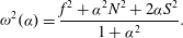 $$\begin{eqnarray}{\it\omega}^{2}({\it\alpha})=\frac{f^{2}+{\it\alpha}^{2}N^{2}+2{\it\alpha}S^{2}}{1+{\it\alpha}^{2}}.\end{eqnarray}$$
For a given medium (
 $\,f,N,S$
), the
 ${\it\alpha}$
minimizing the above equation is
 $$\begin{eqnarray}{\it\alpha}_{m}=\frac{{\it\Omega}_{1}^{2}-{\it\Omega}_{2}^{2}}{2S^{2}},\quad \text{where}~{\it\Omega}_{1}^{2}=N^{2}-f^{2}~\text{and}~{\it\Omega}_{2}^{2}=\sqrt{4S^{4}+{\it\Omega}_{1}^{4}}.\end{eqnarray}$$
Safely assuming
 ${\it\Omega}_{2}\neq 0$
(around which
 ${\it\omega}$
is singular), the minimum frequency is
 $$\begin{eqnarray}{\it\omega}_{m}={\it\omega}({\it\alpha}_{m})=\sqrt{N^{2}+S^{2}/{\it\alpha}_{m}},\end{eqnarray}$$
which is much smaller than
 $N^{2}$
as
 ${\it\alpha}_{m}\ll 1$
. Although (2.7) and (A 4) look very different, their numeric values are equal up to the third significant digit under the parameters used throughout this article. Note also that maximizing equation (A 2) leads to a maximum value for the frequency of
 $\sqrt{N^{2}+2S^{4}/({\it\Omega}_{1}^{2}+{\it\Omega}_{2}^{2})}$
, which is larger than
 $N$
. In any practical case however, the difference is negligible.
The non-hydrostatic expression for the group velocity, equivalent to (2.9), is
 $$\begin{eqnarray}\boldsymbol{c}_{g}=\binom{c_{g}^{\,x}}{c_{g}^{z}}=-\frac{(1-{\it\alpha}^{2})S^{2}+{\it\alpha}(N^{2}-f^{2})}{(1+{\it\alpha}^{2})^{2}m{\it\omega}}\binom{1}{{\it\alpha}}.\end{eqnarray}$$
When
 ${\it\omega}=f$
, (A 2) becomes
 $$\begin{eqnarray}{\it\alpha}_{f}\left[\left(N^{2}-f^{2}\right){\it\alpha}_{f}+2S^{2}\right]=0,\end{eqnarray}$$
which is the equivalent of (2.11). We still have the
 ${\it\alpha}_{f}=0$
solution, while the slope of the steep characteristic becomes
 $$\begin{eqnarray}{\it\alpha}_{f}^{+}=-\frac{2S^{2}}{N^{2}-f^{2}}.\end{eqnarray}$$
When
 ${\it\omega}\neq f$
, solving (A 2) for
 ${\it\alpha}$
yields the counterpart of (2.8):
 $$\begin{eqnarray}{\it\alpha}_{{\it\omega}}^{\pm }=-\frac{S^{2}\mp \sqrt{S^{4}+({\it\omega}^{2}-f^{2})(N^{2}-{\it\omega}^{2})}}{N^{2}-{\it\omega}^{2}}.\end{eqnarray}$$
Appendix B. NIWs at fronts on the non-traditional
$f$
-plane

If non-traditional (NT) terms, namely terms involving the horizontal component of the Earth’s rotation, are retained, then so are the non-hydrostatic terms, without which energy is not conserved.
We now consider waves that propagate purely meridionally, to maximize NT effects. In our two-dimensional configuration, the front is oriented zonally, with denser (lighter) water lying to the North (South). The linearized, inviscid, non-hydrostatic, NT momentum equations now read
 $$\begin{eqnarray}\displaystyle & v_{t}+fu+\left(\tilde{f}+S^{2}/f\right)w=0, & \displaystyle\end{eqnarray}$$
 $$\begin{eqnarray}\displaystyle & w_{t}-b+\tilde{f}v=-p_{z}, & \displaystyle\end{eqnarray}$$
 $\tilde{f}$
is twice the rotation rate of the Earth times the cosine of the latitude. The meridional momentum, continuity and buoyancy equations remain the same. Note that since we have been orienting
 $\hat{\boldsymbol{x}}$
in the direction opposite to the propagation of the waves, the equations above are written in a coordinate system where
 $\hat{\boldsymbol{x}}$
points towards the North and
 $\hat{\boldsymbol{y}}$
points towards the West.
Retracing the steps which led to (2.6) and (A 2), we obtain
 $$\begin{eqnarray}{\it\omega}^{2}=\frac{f^{2}+\left[N^{2}-\left(S^{2}-\tilde{f}f\right)\tilde{f}/f\right]{\it\alpha}^{2}+2\left(S^{2}-\tilde{f}f\right){\it\alpha}}{1+{\it\alpha}^{2}}.\end{eqnarray}$$
If
 $\tilde{f}=0$
, (B 3) is equivalent to (A 2), while if
 $S^{2}=0$
, it is easily deduced from equation (2.8) in Gerkema & Shrira (Reference Gerkema and Shrira2005), with
 $f_{s}=\tilde{f}$
(northward propagation of the waves). In our case, since
 $f$
is approximately equal to the value near the 45° N latitude,
 $\tilde{f}\approx f$
. With the parameters we use, and parameters commonly found in mid-latitude ocean fronts, we have
 $|S|^{2}/N^{2}\approx \tilde{f}f/|S|^{2}\approx 1\,\%$
, and NT (and non-hydrostatic) terms in (A 2) can be neglected. We show this further by illustrating the characteristic slopes with and without NT terms in figure 21, where very little quantitative differences are to be seen between the two cases.
Characteristic slopes
 ${\it\alpha}_{{\it\omega}}^{\pm }$
, for
 ${\it\gamma}=0.3$
(a),
 ${\it\gamma}=1$
(b) and
 ${\it\gamma}=2$
(c), calculated using the frontal parameters used throughout this article (
 $\,f=\tilde{f}=N/100=10^{-4}~\text{s}^{-1}$
,
 $\overline{Ri}=1.05$
). Characteristics calculated with (grey dashed) and without (black) NT effects are virtually identical, indicating that for typical fronts, NT effects do not need to be considered in the physics of critical reflection.

Note that when considering NIWs, the NT terms are comparable with non-hydrostatic terms. Therefore, a study of NIWs in fronts which would include non-hydrostatic effects should also include NT effects, and vice-versa.
Appendix C. Complex demodulation (CD) filtering
Our CD filtering is strongly inspired by the method of Mercier et al. (Reference Mercier, Garnier and Dauxois2008). The filter allows us to both extract the spectral content at a given temporal frequency
 ${\it\omega}$
and then separate the upward- and downward-propagating components (understood in terms of energy propagation) from that signal.
It first extracts the spectral content at the frequency
 ${\it\omega}$
:
 $$\begin{eqnarray}{\it\Xi}_{{\it\omega}}(x,z)=\frac{1}{T}\int _{t_{0}}^{t_{0}+T}{\it\xi}(x,z,t)\exp (-\text{i}{\it\omega}t)\text{d}t,\end{eqnarray}$$
where
 ${\it\Xi}_{{\it\omega}}$
is the component of
 ${\it\xi}$
(namely
 $u$
,
 $v$
,
 $w$
or
 $b$
), oscillating at a frequency
 ${\it\omega}$
,
 $t_{0}$
is a given initial time, and
 $T$
is a duration, which has to be a multiple of
 $2{\rm\pi}/{\it\omega}$
(in practice, ten). In order to retrieve meaningful results, we choose
 $t_{0}$
well after the initial transient phase has ended, which is in practice ten forcing periods. As
 $T$
increases,
 ${\it\Xi}_{{\it\omega}}$
tends towards the value of the temporal Fourier transform of
 ${\it\xi}$
at the frequency
 ${\it\omega}$
.
 ${\it\Xi}_{{\it\omega}}$
is a complex quantity:
 $\text{Re}[{\it\Xi}_{{\it\omega}}\text{e}^{\text{i}{\it\varphi}}]$
, where
 $\text{Re}$
denotes the real part and
 ${\it\varphi}$
a real number, is a reconstruction of the oscillation at a given phase, its modulus
 $|{\it\Xi}_{{\it\omega}}|$
is the amplitude of the oscillation and its argument is the phase of the oscillation. In practice,
 ${\it\xi}$
stands for
 $u$
or
 $w$
and
 ${\it\Xi}$
stands for the corresponding
 $U$
or
 $W$
.
The second step of the CD filter separates the signal into its upward and downward components. First, we numerically compute the spatial discrete Fourier transform (DFT) of
 ${\it\Xi}_{{\it\omega}}$
, which yields
 $\widehat{{\it\Xi}}_{{\it\omega}}(k,m)$
. In the procedure described by Mercier et al. (Reference Mercier, Garnier and Dauxois2008), which is valid for classical internal waves, masks applied on
 $\widehat{{\it\Xi}}_{{\it\omega}}$
isolate upward- and downward-propagating waves, cancelling either positive or negative wavenumbers depending on which quadrant(s) one wants to isolate. Upward and downward spectra will be hereafter referred to as
 $\widehat{{\it\Xi}}_{{\it\omega}}^{u}$
and
 $\widehat{{\it\Xi}}_{{\it\omega}}^{d}$
, respectively, and we have
 $\widehat{{\it\Xi}}_{{\it\omega}}^{u}+\widehat{{\it\Xi}}_{{\it\omega}}^{d}=\widehat{{\it\Xi}}_{{\it\omega}}$
.
For frontal internal waves however, such a procedure is not completely adapted to discriminate incident (upward-propagating) and reflected (downward-propagating) waves, because now the radiation pattern is divided into the eight sectors shown in figure 2. For our simulations, the waves forced by the wave maker are located in sector (3a) of figure 2. If the reflection is forward, the reflected waves are in sector (2a), namely down- and leftward-propagating, such that
 $k<0$
. Similarly to the classical case, incident and reflected vertical wavenumbers have opposite signs and the standard procedure of Mercier et al. (Reference Mercier, Garnier and Dauxois2008) would efficiently separate upward and downward waves. However, if the reflection is backward, the reflected (downward-propagating) waves are located in sector (4b), and the signs of the vertical wavenumber of the incident and backward-reflected waves are identical and thus cannot be discriminated based on the criteria of Mercier et al. (Reference Mercier, Garnier and Dauxois2008). In this specific case of backward-reflected waves, we therefore use the isopycnal slope to isolate the two signals, i.e. our mask cancels either the wavevectors for which
 $k>S^{2}m/N^{2}$
or for which
 $k<S^{2}m/N^{2}$
, which yields
 $\widehat{{\it\Xi}}_{{\it\omega}}^{u}$
and
 $\widehat{{\it\Xi}}_{{\it\omega}}^{d}$
, respectively.
At each step of the CD filtering algorithm, we use the crudest masks and windows, for example the first time integral (C 1) amounts to computing a Fourier transform with a rectangular window, which is ten forcing periods wide. Because the signal is mostly periodic, significant distortion of the signal is not to be expected. The direct and inverse DFTs are computed without taking into account that the signal is not periodic in the vertical; however this does not qualitatively affect the results. Likewise, the masks applied to
 $\widehat{{\it\Xi}}_{{\it\omega}}$
do not include any windowing and yet do not induce distortions strong enough to affect our conclusions.