

I. INTRODUCTION
Irving Fisher’s achievements as one of America’s most accomplished economists are generally well known.Footnote 1 Yet there is much that is not widely recognized about his contributions to index number theory: the focus of the present paper. But before we look at his contributions to this subject, it will be useful to list the areas of research that Fisher himself thought were of some importance near the end of his life.
In 1946, Fisher gave an address on the founding of the Irving Fisher Foundation, a foundation he set up to continue research in areas that he pursued over his productive life. This address was later published as Fisher Reference Fisher, Barber, Dimand and Foster(1997), and we will review the research that Fisher flagged as important areas where he had contributed and that he hoped the foundation would continue to explore.
Fisher (1997, pp. 23–36) listed the following seven research areas:
• the basic principles of economic science;
• monetary stabilization;
• the consumption tax;
• general economics;
• world peace;
• health habitsFootnote 2; and
• eugenics.
The last three topics can best be left to others to discuss in more detail but a few sentences about the first four topics follow below.
Fisher summarized his work on the first topic as follows:
One of my chief objects has been to help make economics into a genuine science through careful and sound analysis, usually carried out with the help of mathematical methods and statistical verification. My chief books written with this object in view are: The thesis just mentioned, 1892; The Nature of Capital and Income, 1906; The Purchasing Power of Money, 1911; The Theory of Interest, 1930; Booms and Depressions, 1932. (Fisher Reference Fisher, Barber, Dimand and Foster1997, p. 23)
Fisher’s doctoral thesis at Yale had the title Mathematical Investigations in the Theory of Value and Prices and it was an early study in the mathematics of general equilibrium theory.Footnote 3 There is no doubt that Fisher’s contributions to the development of a modern theory of the interest rate in a general equilibrium context were seminal and are still used in introductory economics courses today. His work on operationalizing the quantity theory of money is still relevant today, and it was this work that led him to attempt to measure general inflation, and this, in turn, led him into index number theory.
Fisher’s second listed area of interest was monetary stabilization. He had a keen sense of the injustices that resulted from unanticipated inflation in the context of debt contracts:
In all mathematical sciences, the first essential is a unit for measurement. The lack of such a unit for measuring the value of money in the sense of its purchasing power soon impressed me. Several times within my life the dollar has more than doubled or been more than halved in value. Yet throughout all these vicissitudes, only a handful of people had the slightest idea of what was happening. (Fisher Reference Fisher, Barber, Dimand and Foster1997, p. 23)
Fisher’s solution to the injustices generated by unanticipated rates of inflation was to index interest rates to the rate of inflation, and so the measurement of general inflation became an important practical problem.Footnote 4 Fisher felt strongly about this problem, and wrote six books and hundreds of articles on the problem of monetary stabilization and indexation.Footnote 5
Fisher’s third listed area was the consumption tax, which Fisher (1997, p. 28) called the spending tax. He felt that savings should not be taxed, partly because he felt this led to double taxation (if there were consumption taxes in addition to savings taxes) and partly because of the adverse efficiency and growth effects of taxing interest:
In several books (especially The Nature of Capital and Income, 1906, and Constructive Income Taxation, 1942) as well as in many articles, I have endeavored to show that, whenever part of an income is saved and thus becomes capital, a tax on that part, followed by a like tax on the subsequent income from that capital, amounts to double taxation.... I have shown that, had our present income tax been in existence at the beginning of the century, industrial progress could not have been as rapid as it was ... for the resulting tax on savings (from which we now suffer) would have substantially reduced corporate savings—and a reduction of corporate savings is a reduction of expansion. (Fisher Reference Fisher, Barber, Dimand and Foster1997, p. 28)
Thus, Fisher was a strong advocate of a consumption tax as opposed to an income tax.
Fisher’s fourth listed area was general economics. What Fisher had in mind here was the study of economic efficiency and its trade-off with possible inequalities in income and wealth:
In our efforts to improve distribution we must not impair production—must, in fact, improve it. As my first teacher in economics, Professor William Graham Sumner, often said, we can accomplish more by levelling up than by levelling down, meaning that most efforts ‘to soak the rich’ do not help but rather harm the poor by reducing production. (Fisher Reference Fisher, Barber, Dimand and Foster1997, p. 30)
But Fisher was concerned that the non-taxation of savings might lead to large disparities in wealth over time, and suggested some solutions to this problem:
In line with this thought I have stressed two measures: (1) exempt all savings from income taxes, for savings in general mean added capital equipment and this means greater production.... (2) tax the savings only when they pass out of the hands of the accumulator, that is (chiefly) on his death; ... (3) during life, tax all progressively on excessive spending, that is on their disaccumulations. (Fisher Reference Fisher, Barber, Dimand and Foster1997, p. 30)
Thus, to compensate for the lack of taxation on savings, Fisher advocated a progressive consumption tax along with an inheritance tax.Footnote 6
The above material gives us some indication of why Fisher became interested in index number theory: it was a consequence of his interest in using economics (and statistics) to improve society.
In order to evaluate Fisher’s lasting contributions to index number theory, it will be useful to give the reader a review of the current state of index number theory. There are four main approaches to index number theory that are widely used todayFootnote 7:
• the fixed basket approach;
• the stochastic approach;
• the test approach; and
• the economic approach.
Thus, in sections III–VI below, we review each of these approaches (and note Fisher’s contributions to these approaches). However, before discussing these approaches, in section II we present a preliminary discussion on the levels approach to index number theory versus the value ratio decomposition approach (with the latter approach being the one that Fisher followed).
In section VII, we discuss why Fisher was opposed to the stochastic and economic approaches to index number theory. In section VIII, we will discuss Fisher’s contributions to multilateral index number theory. The issue of whether to use fixed base or chained index numbers arises in this context, so, in section VIII, we also discuss Fisher’s thoughts on this issue. Section IX concludes.
II. THE LEVELS AND VALUE RATIO APPROACHES TO INDEX NUMBER THEORY
It will be useful to follow the example of Fisher (1922, p. 8) and set the stage for the subsequent discussion of alternative approaches by more precisely defining the index number problem.
We specify two accounting periods,Footnote 8t = 0,1, for which we have micro price and quantity data for N commodities pertaining to transactions by a consumer or producer (or a well-defined group of consumers or producers). Denote the price and quantity of commodity n in period t by  $p_n^t$ and
 $q_n^t$, respectively, for n = 1, 2, …, N and t = 0,1. Before proceeding further, we need to discuss the exact meaning of the microeconomic prices and quantities if there are multiple transactions for, say, commodity n within period t. In this case, it is natural to interpret
 $q_n^t$ as the total amount of commodity n transacted within period t. In order to conserve the value of transactions, it is necessary that
 $p_n^t$ be defined as a unit value Footnote 9; i.e.,
 $p_n^t$ must be equal to the value of transactions for commodity n during period t divided by the total quantity transacted,
 $q_n^t$. For t = 0,1, define the value of transactions in period t as:
 $$V^t \equiv \sum\nolimits_{n = 1}^N {p_n^t q_n^t \equiv p^t \cdot q^t }$$
where 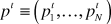 $p^t \equiv \left( {p_1^2 , \ldots ,p_N^t } \right)$ is the period t price vector,
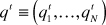 $q^t \equiv \left( {q_1^t , \ldots ,q_N^t } \right)$ is the period t quantity vector, and p t⋅q t denotes the inner product of these two vectors.
Using the above notation, we can now state the following levels version of the index number problem using the test or axiomatic approach: for t = 0,1, find scalar numbers P t and Q t such that
 $$V^t = P^t Q^t .$$
The number P t is interpreted as an aggregate period t price level while the number Q t is interpreted as an aggregate period t quantity level. The aggregate price level P t is allowed to be a function of the period t price vector, p t while the aggregate period t quantity level Q t is allowed to be a function of the period t quantity vector, q t; i.e., we have
 $$P^t = c\left( {p^t } \right)\;{\rm{and}}\;Q^t = f\left( {q^t } \right)\;;\;t = 0,1.$$
However, from the viewpoint of the test approach to index number theory, the levels approach to finding aggregate quantities and prices comes to an abrupt halt: Eichhorn (1978, p. 144) showed that if the number of commodities N in the aggregate is equal to or greater than 2, and we restrict c(p t) and f(q t) to be positive if the micro prices and quantities  $p_n^t$ and
 $q_n^t$ are positive, then there do not exist any functions c and f such that c(p t)f(q t) = p t⋅q t for all p t >> 0N and q t >> 0N.Footnote 10
This negative result can be reversed if we take the economic approach to index number theory. In this approach, we assume that the economic agent has a linearly homogeneous utility function, f(q), and, when facing the prices p t chooses q t to solve the following cost-minimization problem:
 $$\min _q \left\{ {p^t \cdot q\;:\;p^t \cdot q = Y^t \;;\;q \ge 0_N } \right\}\;;\;t = 0,1$$
where period t “income” Y t is defined as p t⋅q t. In this setup, it turns out that c(p) is the unit cost function that is dualFootnote 11 to the linearly homogeneous utility function f(q), and we can define P t and Q t as in (3) with P tQ t = c(p t)f(q t) = p t⋅q t for t = 0,1. Why does the economic approach work in the levels version of the index number problem, whereas the test approach does not? In the test approach, both p t and q t are regarded as completely independent variables, whereas in the economic approach, p t can vary independently but q t cannot vary independently; it is a solution to the period t cost-minimization problem (4).
Even though the economic approach to the index number problem as formulated above “works,” it is not a practical solution that statistical agencies can implement and provide suitable aggregates to the public. In order to implement this solution, the statistical agency would have to hire hundreds of econometricians in order to estimate cost functions for all relevant macroeconomic aggregates, and it is simply not feasible to do this. Thus, we turn to our second formulation of the index number problem, and it is this formulation that was initiated by Fisher (Reference Fisher1911, Reference Fisher1922) in his two books on index number theory.
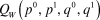
In the second approach to index number theory, instead of trying to decompose the value of the aggregate into price and quantity components for a single period, we instead attempt to decompose a value ratio for the two periods under consideration into a price change component P times a quantity change component Q.Footnote 12 Thus, we now look for two functions of 4N variables, P(p 0, p 1, q 0, q 1) and Q(p 0, p 1, q 0, q 1) such thatFootnote 13:
 $${{p^1 \cdot q^1 } \mathord{\left/ {\vphantom {{p^1 \cdot q^1 } {p^0 \, \cdot {\kern 1pt} q^0 }}} \right. \kern-\nulldelimiterspace} {p^0 \, \cdot {\kern 1pt} q^0 }} = P\left( {p^0 ,{\kern 1pt} p^1 ,{\kern 1pt} q^0 ,{\kern 1pt} q^1 } \right)Q\left( {p^0 ,{\kern 1pt} p^1 ,{\kern 1pt} q^0 ,{\kern 1pt} q^1 } \right).$$
If we take the test approach, then we want equation (5) to hold for all positive price and quantity vectors pertaining to the two periods under consideration, p 0, p 1, q 0, q 1. If we take the economic approach, then only the price vectors p 0 and p 1 are regarded as independent variables, while the quantity vectors, q 0 and q 1, are regarded as dependent variables.
In this second approach to index number theory, the price index P(p 0, p 1, q 0, q 1) and the quantity index Q(p 0, p 1, q 0, q 1) cannot be determined independently; i.e., if either one of these two functions is determined, then the remaining function is implicitly determined using equation (5). Historically, the focus has been on the determination of the price index but Fisher (1911, p. 388) was the first to realize that once the price index was determined, then equation (5) could be used to determine the companion quantity index.Footnote 14 Fisher (1911, p. 401) also realized that one could assume that Q had certain properties or satisfied certain tests and that these quantity tests would imply that the companion price index defined via (5) would then satisfy some interesting properties or tests that were not immediately evident. Thus, it can already be seen that Fisher made some fundamental contributions to index number theory.Footnote 15
This value ratio decomposition approach to index number theory is called bilateral index number theory and its focus is the determination of “reasonable” functional forms for P and Q. Fisher’s Reference Fisher1911 and Reference Fisher1922 books address this functional form issue using the test approach.
We turn now to a discussion of the various approaches that have been used to determine the functional form for the bilateral price index, P(p 0, p 1, q 0, q 1).
III. FIXED BASKET APPROACHES TO INDEX NUMBER THEORY
A very simple approach to the determination of a price index over a group of commodities is the fixed basket approach. In this approach, we are given a basket of commodities that is represented by the positive quantity vector q. Given the price vectors for periods 0 and 1, p 0 and p 1, respectively, we can calculate the cost of purchasing this same basket in the two periods, p 0⋅q and p 1⋅q. Then the ratio of these costs is a very reasonable indicator of pure price change over the two periods under consideration, provided that the basket vector q is “representative.” Thus, define the Lowe price index, P Lo, as follows:
 $$P_{Lo} \left( {p^0 ,p^1 ,q} \right) \equiv {{p^1 \cdot q} \mathord{\left/ {\vphantom {{p^1 \cdot q} {p^0 \cdot q}}} \right. \kern-\nulldelimiterspace} {p^0 \cdot q}}.$$
Although Lowe (Reference Lowe1823) was not the first to suggest this form of price index,Footnote 16 he considered the problems associated with its construction and the uses that it could be put to in much more detail than his precursors:
Of this, some idea may be formed from a table in the Appendix comprising a list of articles of general consumption, corn, butcher-meat, manufactures, tropical products, &c. and containing the probable amount of money expended on each by the public. This table is followed by explanatory remarks, of which the object is to show that contracts for a series of years ought to be made with a reference to the power of money in purchasing the necessaries and comforts of life; that after fixing a given sum, say 100l. as the amount of an annual salary, the payment in subsequent years should be not necessarily 100l., but either 95l., 100l., or 105l., according to the varying power of money in making purchases…. For the details of the table, and the calculations connected with it, we refer to the Appendix: at present we shall, for the sake of illustration, suppose it in operation, and bestow a few paragraphs on the effects that the adoption of such a measure would have on the interests of the country. In what, it may be asked, would the benefits of it consist? In ascertaining on grounds that would admit of no doubt or dispute, the power in purchase of any given sum in one year, compared to its power of purchase in another. And what would be the practical application of this knowledge? The correction of a long list of anomalies in regard to rents, salaries, wages, &c., arising out of unforeseen fluctuations in our currency. (Lowe Reference Lowe1823, pp. 333–335)
It can be seen that Lowe laid out a fairly modern theory for the construction of a Consumer Price Index.Footnote 17 In order that the basket vector be “representative,” Lowe (1823, Appendix p. 95) suggested that the commodity basket vector q should be updated every five years. Lowe was also concerned with the problem of the unfairness of unforeseen changes in the price level on fixed interest contracts that concerned Fisher, and, in fact, Fisher (1911, p. 248) refers to Lowe’s path-breaking book.Footnote 18
As time passed, economists and price statisticians demanded a bit more precision with respect to the specification of the basket vector q. There are two natural choices for the reference basket: the period 0 commodity vector q 0 or the period 1 commodity vector q 1. These two choices lead to the Laspeyres (Reference Laspeyres1871) price index P L defined by (7) and the Paasche (Reference Paasche1874) price index P P defined by (8)Footnote 19:
 $$P_L \left( {p^0 ,p^1 ,q^0 ,q^1 } \right) \equiv {{p^1 \cdot q^0 } \mathord{\left/ {\vphantom {{p^1 \cdot q^0 } {p^0 \cdot q^0 }}} \right. \kern-\nulldelimiterspace} {p^0 \cdot q^0 }} = \sum\nolimits_{n = 1}^N {s_n^0 \left( {{{p_n^1 } \mathord{\left/ {\vphantom {{p_n^1 } {p_n^0 }}} \right. \kern-\nulldelimiterspace} {p_n^0 }}} \right)} ;$$
 $$P_P \left( {p^0 ,p^1 ,q^0 ,q^1 } \right) \equiv {{p^1 \cdot q^1 } \mathord{\left/ {\vphantom {{p^1 \cdot q^1 } {p^0 \cdot q^1 }}} \right. \kern-\nulldelimiterspace} {p^0 \cdot q^1 }} = \left[ {\sum\nolimits_{n = 1}^N {s_n^1 \left( {{{p_n^1 } \mathord{\left/ {\vphantom {{p_n^1 } {p_n^0 }}} \right. \kern-\nulldelimiterspace} {p_n^0 }}} \right)^{ - 1} } } \right]^{ - 1} $$
where the period t expenditure share on commodity n,  $s_n^t$, is defined as
 ${{p_n^t q_n^t } \mathord{\left/ {\vphantom {{p_n^t q_n^t } {p^t \cdot q^t }}} \right. \kern-\nulldelimiterspace} {p^t \cdot q^t }}$ for n = 1,…,N and t = 0,1. Thus, the Laspeyres price index P L can be written as a base period expenditure share weighted average of the N price ratios (or price relatives),
 ${{p_n^1 } \mathord{\left/ {\vphantom {{p_n^1 } {p_n^0 }}} \right. \kern-\nulldelimiterspace} {p_n^0 }}$.Footnote 20 The last equation in (8) shows that the Paasche price index P P can be written as a period 1 (or current period) expenditure share weighted harmonic average of the N price ratios.Footnote 21
One problem with these index number formulae is that they are equally plausible but, in general, they will give different answers. This suggests that if we require a single estimate for the price change between the two periods, then we should take some sort of evenly weighted average of the two indexes as our final estimate of price change between periods 0 and 1. Examples of such symmetric averages are the arithmetic mean, which leads to the Drobisch (Reference Drobisch1871) Sidgwick (1883, p. 68) Bowley (1901, p. 227)Footnote 22 index, (1/2)P L + (1/2)P P, and the geometric mean, which leads to the Fisher Footnote 23 (1922) ideal index, P F, defined as
 $$P_F \left( {p^0 ,p^1 ,q^0 ,q^1 } \right) \equiv \left[ {P_L \left( {p^0 ,p^1 ,q^0 ,q^1 } \right)P_P \left( {p^0 ,p^1 ,q^0 ,q^1 } \right)} \right]^{{1 \mathord{\left/ {\vphantom {1 2}} \right. \kern-\nulldelimiterspace} 2}} .$$
At this point, the fixed basket approach to index number theory has to draw on the test approach to index number theory; i.e., in order to determine which of these fixed basket indexes or which averages of them might be “best,” we need criteria or tests or properties that we would like our indexes to satisfy.
Let a and b be two positive numbers. A mean or an average of the two numbers a and b is a function m(a, b) that has certain properties, the most important of which is the property m(a, a) = a; i.e., if the two numbers are the same, then the mean function is equal to this common number. Diewert (1993b, p. 361) defined a symmetric homogeneous mean of a and b as a function m(a, b) that has the following properties: m(a, a) = a for all a> 0; m(a, b) is a continuous and increasing function of a and b; m(a, b) = m(b, a) for all a and b and m(λa, λb) = λm(a, b) for all positive a, b, and λ.
What is the “best” symmetric average of P L and P P to use as a point estimate for the theoretical cost of living index? It is very desirable for a price index formula that depends on the price and quantity vectors pertaining to the two periods under consideration to satisfy the time reversal test.Footnote 24 We say that the index number formula P(p 0, p 1, q 0, q 1) satisfies this test if
 $$P\left( {p^1 ,p^0 ,q^1 ,q^0 } \right) = {1 \mathord{\left/ {\vphantom {1 {P\left( {p^0 ,p^1 ,q^0 ,q^1 } \right)}}} \right. \kern-\nulldelimiterspace} {P\left( {p^0 ,p^1 ,q^0 ,q^1 } \right)}};$$
i.e., if we interchange the period 0 and period 1 price and quantity data and evaluate the index, then this new index P(p 1, p 0, q 1, q 0) is equal to the reciprocal of the original index P(p 0, p 1, q 0, q 1).
Diewert (1997, p. 138) showed that the Fisher ideal price index defined by (9) above is the only index that is a homogeneous symmetric mean of the Laspeyres and Paasche price indexes, P L and P P, and satisfies the time reversal test (10) above. Thus, our first symmetric basket approach to bilateral index number theory leads to the Fisher index (9) as being “best” from the perspective of this approach.Footnote 25
Instead of looking for a “best” average of the two fixed basket indexes that correspond to the baskets chosen in either of the two periods being compared, we could instead look for a “best” average basket of the two baskets represented by the vectors q 0 and q 1 and then use this average basket to compare the price levels of periods 0 and 1.Footnote 26 Thus, we ask that the nth quantity weight, q n, be an average or mean of the base period quantity  $q_n^0 $ and the period 1 quantity for commodity n
 $q_n^1$, say
 $m\left( {q_n^0 ,q_n^1 } \right)$, for n = 1,2,…,N.Footnote 27 Price statisticians refer to this type of index as a pure price index and it corresponds to Knibbs’ (1924, p. 43) unequivocal price index. Under these assumptions, the pure price index can be defined as a member of the following class of index numbers:
 $$P_K \left( {p^0 ,p^1 ,q^0 ,q^1 } \right) \equiv {{\sum\nolimits_{n = 1}^N {{\rm{p}}_n^1 m\left( {q_n^0 ,q_n^1 } \right)} } \mathord{\left/ {\vphantom {{\sum\nolimits_{n = 1}^N {{\rm{p}}_n^1 m\left( {q_n^0 ,q_n^1 } \right)} } {\sum\nolimits_{j = 1}^N {p_j^0 m\left( {q_j^0 ,q_j^1 } \right)} }}} \right. \kern-\nulldelimiterspace} {\sum\nolimits_{j = 1}^N {p_j^0 m\left( {q_j^0 ,q_j^1 } \right)} }}.$$
In order to determine the functional form for the mean function m, it is necessary to impose some tests or axioms on the pure price index defined by (11). Again we ask that P K satisfy the time reversal test, (10), above. Under this hypothesis, it can be shown that m must be a symmetric mean; i.e., m must satisfy the following property: m(a, b) = m(b, a) for all a > 0 and b > 0.
The assumption that m must be a symmetric mean still does not pin down the functional form for the pure price index defined by (13) above. For example, the function m(a, b) could be the arithmetic mean, (1/2)a + (1/2)b, in which case (11) reduces to the Marshall (1887) Edgeworth (1925) price index P ME, which was the pure price index preferred by Knibbs (1924, p. 56):
 $$P_{ME} \left( {p^0 ,p^1 ,q^0 ,q^1 } \right) \equiv {{\sum\nolimits_{n = 1}^N {p_n^1 \left( {{1 \mathord{\left/ {\vphantom {1 2}} \right. \kern-\nulldelimiterspace} 2}} \right)\left( {q_n^0 + q_n^1 } \right)} } \mathord{\left/ {\vphantom {{\sum\nolimits_{n = 1}^N {p_n^1 \left( {{1 \mathord{\left/ {\vphantom {1 2}} \right. \kern-\nulldelimiterspace} 2}} \right)\left( {q_n^0 + q_n^1 } \right)} } {\sum\nolimits_{j = 1}^N {p_j^0 \left( {{1 \mathord{\left/ {\vphantom {1 2}} \right. \kern-\nulldelimiterspace} 2}} \right)\left( {q_j^0 + q_j^1 } \right)} .}}} \right. \kern-\nulldelimiterspace} {\sum\nolimits_{j = 1}^N {p_j^0 \left( {{1 \mathord{\left/ {\vphantom {1 2}} \right. \kern-\nulldelimiterspace} 2}} \right)\left( {q_j^0 + q_j^1 } \right)} .}}$$
On the other hand, the function m(a,b) could be the geometric mean, (ab)1/2, in which case (11) becomes the Walsh (1901, p. 398; 1921a, p. 97) price index, P WFootnote 28:
 $$P_W \left( {p^0 ,p^1 ,q^0 ,q^1 } \right) \equiv {{\sum\nolimits_{n = 1}^N {p_n^1 \left( {q_n^0 q_n^1 } \right)^{{1 \mathord{\left/ {\vphantom {1 2}} \right. \kern-\nulldelimiterspace} 2}} } } \mathord{\left/ {\vphantom {{\sum\nolimits_{n = 1}^N {p_n^1 \left( {q_n^0 q_n^1 } \right)^{{1 \mathord{\left/ {\vphantom {1 2}} \right. \kern-\nulldelimiterspace} 2}} } } {\sum\nolimits_{j = 1}^N {p_j^0 \left( {q_j^0 q_j^1 } \right)^{{1 \mathord{\left/ {\vphantom {1 2}} \right. \kern-\nulldelimiterspace} 2}} } }}} \right. \kern-\nulldelimiterspace} {\sum\nolimits_{j = 1}^N {p_j^0 \left( {q_j^0 q_j^1 } \right)^{{1 \mathord{\left/ {\vphantom {1 2}} \right. \kern-\nulldelimiterspace} 2}} } }}.$$
However, there are many other possibilities for the mean function m, including the mean of order r, [(1/2)a r + (1/2)b r ]1/r for r ≠ 0. Obviously, in order to completely determine the functional form for the pure price index P K, we need to impose at least one additional test or axiom on P K(p 0, p 1, q 0, q 1).
In order to obtain an additional axiom, we note that there is a problem with the use of the Marshall Edgeworth price index (12) in the context of using the formula to make international comparisons of prices. If the prices of a very large country are compared to the prices of a small country, using formula (12), then the quantity vector of the large country may totally overwhelm the influence of the quantity vector corresponding to the small country. In technical terms, the Marshall Edgeworth formula is not homogeneous of degree 0 in the components of both q 0 and q 1. As one way of preventing this problem from occurring, we could ask that P K defined by (11) satisfy the following invariance to proportional changes in current quantities test:
 $$P\left( {p^0 ,p^1 ,q^0 ,\lambda q^1 } \right) = P\left( {p^0 ,p^1 ,q^0 ,q^1 } \right)\;{\rm{for}}\;{\rm{all}}\;\lambda > 0.$$
It can be shown that these two tests, the time reversal test (10) and the invariance test (14), enable us to determine the precise functional form for the pure price index P K defined by (11) above where m is a symmetric homogeneous mean: the pure price index P K must be the Walsh index P W defined by (13).Footnote 29
Thus, the fixed basket approach to bilateral index number theory starts out with the Laspeyres and Paasche price indexes. Some form of averaging of these two indexes is called for, since both indexes are equally plausible. Averaging these two indexes directly leads to the Fisher ideal index P F defined by (9) as being “best,” while a direct averaging of the two quantity baskets q 0 and q 1 leads to the Walsh price index P W defined by (13) as being “best.”
We turn now to another early approach to the index number problem.
IV. STOCHASTIC AND DESCRIPTIVE STATISTICS APPROACHES TO INDEX NUMBER THEORY
The (unweighted) stochastic approach to the determination of the price index can be traced back to the work of Jevons (Reference Jevons1865, Reference Jevons1884) and Edgeworth (Reference Edgeworth1888, Reference Edgeworth1896, Reference Edgeworth1901) over a hundred years ago.Footnote 30
The basic idea behind the stochastic approach is that each price relative,  ${{p_n^1 } \mathord{\left/ {\vphantom {{p_n^1 } {p_n^0 }}} \right. \kern-\nulldelimiterspace} {p_n^0 }}$ for n = 1, 2, …, N, can be regarded as an estimate of a common inflation rate α between periods 0 and 1; i.e., Jevons and Edgeworth essentially assumed that
 $${{p_n^1 } \mathord{\left/ {\vphantom {{p_n^1 } {p_n^0 = \alpha + \varepsilon _n \;;\;n = 1,2, \ldots ,N}}} \right. \kern-\nulldelimiterspace} {p_n^0 = \alpha + \varepsilon _n \;;\;n = 1,2, \ldots ,N}}$$
where α is the common inflation rate and the ε n are random variables with mean 0 and variance σ 2. The least squares estimator for α is the Carli (1804) price index P C defined as
 $$P_C \left( {p^0 ,p^1 } \right) \equiv \sum\nolimits_{n = 1}^N {\left( {{1 \mathord{\left/ {\vphantom {1 N}} \right. \kern-\nulldelimiterspace} N}} \right)\left( {{{p_n^1 } \mathord{\left/ {\vphantom {{p_n^1 } {p_n^0 }}} \right. \kern-\nulldelimiterspace} {p_n^0 }}} \right)} .$$
Unfortunately, P C does not satisfy the time reversal test; i.e., P C(p 1, p 0) ≠ 1/P C(p 0, p 1)Footnote 31.
Now assume that the logarithm of each price relative,  $ln\left( {{{p_n^1 } \mathord{\left/ {\vphantom {{p_n^1 } {p_n^0 }}} \right. \kern-\nulldelimiterspace} {p_n^0 }}} \right)$, is an independent unbiased estimate of the logarithm of the inflation rate between periods 0 and 1, β, say. Thus, we have:
 $$ln\left( {{{p_n^1 } \mathord{\left/ {\vphantom {{p_n^1 } {p_n^0 }}} \right. \kern-\nulldelimiterspace} {p_n^0 }}} \right) = \beta + \varepsilon _n \;;\;n = 1,2, \ldots N$$
where β ≡ lnα and the ε n are independently distributed random variables with mean 0 and variance σ 2. The least squares or maximum likelihood estimator for β is the logarithm of the geometric mean of the price relatives. Hence, the corresponding estimate for the common inflation rate α is the Jevons (1865) price index P J defined as:
 $$P_J \left( {p^0 ,p^1 } \right) \equiv \prod\nolimits_{n = 1}^N {\left( {{{p_n^1 } \mathord{\left/ {\vphantom {{p_n^1 } {p_n^0 }}} \right. \kern-\nulldelimiterspace} {p_n^0 }}} \right)^{{1 \mathord{\left/ {\vphantom {1 N}} \right. \kern-\nulldelimiterspace} N}} } .$$
The Jevons price index P J does satisfy the time reversal test and, hence, is much more satisfactory than the Carli index P C. However, both the Jevons and Carli price indexes suffer from a fatal flaw: each price relative  ${{p_n^1 } \mathord{\left/ {\vphantom {{p_n^1 } {p_n^0 }}} \right. \kern-\nulldelimiterspace} {p_n^0 }}$ is regarded as being equally important and is given an equal weight in the index number formulae (16) and (18).Footnote 32 Keynes (1930, pp. 76–81) also criticized the unweighted stochastic approach to index number theory on two other grounds: (i) price relatives are not distributed independently, and (ii) there is no single inflation rate that can be applied to all parts of an economy; e.g., Keynes demonstrated empirically that wage rates, wholesale prices, and final consumption prices all had different rates of inflation. In order to overcome the Keynesian criticisms of the unweighted stochastic approach to index numbers, it is necessary to:
• have a definite domain of definition for the index number; and
• weight the price relatives by their economic importance.
Theil (1967, pp. 136–137) proposed a solution to the lack of weighting in (17). He argued as follows. Suppose we draw price relatives at random in such a way that each dollar of expenditure in the base period has an equal chance of being selected. Then the probability that we will draw the nth price relative is equal to  $s_n^0 \equiv {{p_n^0 q_n^0 } \mathord{\left/ {\vphantom {{p_n^0 q_n^0 } {p^0 \cdot q^0 }}} \right. \kern-\nulldelimiterspace} {p^0 \cdot q^0 }}$, the period 0 expenditure share for commodity n. Then the overall mean (period 0 weighted) logarithmic price change is
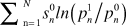 $\sum\nolimits_{{\rm{n}} = 1}^N {s_n^0 ln\left( {{{p_n^1 } \mathord{\left/ {\vphantom {{p_n^1 } {p_n^0 }}} \right. \kern-\nulldelimiterspace} {p_n^0 }}} \right)} $. Now repeat the above mental experiment and draw price relatives at random in such a way that each dollar of expenditure in period 1 has an equal probability of being selected. This leads to the overall mean (period 1 weighted) logarithmic price change of
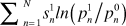 $\sum\nolimits_{n = 1}^N {s_n^1 ln\left( {{{p_n^1 } \mathord{\left/ {\vphantom {{p_n^1 } {p_n^0 }}} \right. \kern-\nulldelimiterspace} {p_n^0 }}} \right)} $. Each of these measures of overall logarithmic price change seems equally valid so we could argue for taking a symmetric average of the two measures in order to obtain a final single measure of overall logarithmic price change. Theil (1967, p. 137) argued that a nice symmetric index number formula can be obtained if we make the probability of selection for the nth price relative equal to the arithmetic average of the period 0 and 1 expenditure shares for commodity n. Using these probabilities of selection, Theil’s final measure of overall logarithmic price change is
 $$lnP_T \left( {p^0 ,p^1 ,q^0 ,q^1 } \right) \equiv \sum\nolimits_{n = 1}^N {\left( {{1 \mathord{\left/ {\vphantom {1 2}} \right. \kern-\nulldelimiterspace} 2}} \right)\left( {s_n^0 + s_n^1 } \right)ln\left( {{{p_n^1 } \mathord{\left/ {\vphantom {{p_n^1 } {p_n^0 }}} \right. \kern-\nulldelimiterspace} {p_n^0 }}} \right)} .$$
It is possible to give a descriptive statistics interpretation of the right-hand side of (19). Define the nth logarithmic price ratio r n by:
 $$r_n \equiv ln\left( {{{p_n^1 } \mathord{\left/ {\vphantom {{p_n^1 } {p_n^0 }}} \right. \kern-\nulldelimiterspace} {p_n^0 }}} \right)\quad {\rm{ for}}\;n = 1, \ldots ,N.$$
Now define the discrete random variable, R, say, as the random variable that can take on the values r n with probabilities  $\rho _n \equiv \left( {{1 \mathord{\left/ {\vphantom {1 2}} \right. \kern-\nulldelimiterspace} 2}} \right)\left( {s_n^0 + s_n^1 } \right)$ for n = 1, …, N. Note that since each set of expenditure shares,
 $s_n^0 $ and
 $s_n^1 $, sums to one, the probabilities ρ n will also sum to one. It can be seen that the expected value of the discrete random variable R is lnP T(p 0, p 1, q 0, q 1) as defined by the right-hand side of (19). Thus, the logarithm of the index P T can be interpreted as the expected value of the distribution of the logarithmic price ratios in the domain of definition under consideration, where the N discrete price ratios in this domain of definition are weighted according to Theil’s probability weights, ρ n.
Taking antilogs of both sides of (19), we obtain the Theil price index, P T.Footnote 33 This index number formula has a number of good properties. In particular, P T satisfies the time reversal test (10) and the linear homogeneity test (14).Footnote 34
It is possible to consider a descriptive statistics approach to index number theory where we look at the distribution of price ratios, ${{p_n^1 } \mathord{\left/ {\vphantom {{p_n^1 } {p_n^0 }}} \right. \kern-\nulldelimiterspace} {p_n^0 }}$, rather than the distribution of the logarithmic price ratios,
 $ln\left( {{{p_n^1 } \mathord{\left/ {\vphantom {{p_n^1 } {p_n^0 }}} \right. \kern-\nulldelimiterspace} {p_n^0 }}} \right)$. Thus, following in the footsteps of Theil leads to price indexes of the form
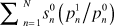 $\sum\nolimits_{n = 1}^N {s_n^0 \left( {{{p_n^1 } \mathord{\left/ {\vphantom {{p_n^1 } {p_n^0 }}} \right. \kern-\nulldelimiterspace} {p_n^0 }}} \right)} $,
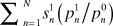 $\sum\nolimits_{n = 1}^N {s_n^1 \left( {{{p_n^1 } \mathord{\left/ {\vphantom {{p_n^1 } {p_n^0 }}} \right. \kern-\nulldelimiterspace} {p_n^0 }}} \right)} $ and more generally of the form:
 $$P_m \left( {p^0 ,p^1 ,q^0 ,q^1 } \right) \equiv \sum\nolimits_{n = 1}^N {m\left( {s_n^0 ,s_n^1 } \right)\left( {{{p_n^1 } \mathord{\left/ {\vphantom {{p_n^1 } {p_n^0 }}} \right. \kern-\nulldelimiterspace} {p_n^0 }}} \right)} $$
where  $m\left( {s_n^0 ,s_n^1 } \right)$ is a homogeneous symmetric mean of the period 0 and 1 expenditure shares,
 $s_n^0 $ and
 $s_n^1 $. In order to interpret the right-hand side of (21) as an expected value of the price ratios
 ${{p_n^1 } \mathord{\left/ {\vphantom {{p_n^1 } {p_n^0 }}} \right. \kern-\nulldelimiterspace} {p_n^0 }}$, it is necessary that
 $$\sum\nolimits_{n = 1}^N {m\left( {s_n^0 ,s_n^1 } \right)} = 1.$$
However, in order to satisfy (22), m cannot be a symmetric geometric or harmonic mean or any of the commonly used homogeneous symmetric means. In fact, the only simple homogeneous symmetric mean that satisfies (22) is the arithmetic mean. With this choice of m, (21) becomes the following (unnamed) index number formula, P u:
 $$P_u \left( {p^0 ,p^1 ,q^0 ,q^1 } \right) \equiv \sum\nolimits_{n = 1}^N {\left( {{1 \mathord{\left/ {\vphantom {1 2}} \right. \kern-\nulldelimiterspace} 2}} \right)\left( {s_n^0 ,s_n^1 } \right)\left( {{{p_n^1 } \mathord{\left/ {\vphantom {{p_n^1 } {p_n^0 }}} \right. \kern-\nulldelimiterspace} {p_n^0 }}} \right)} .$$
Unfortunately, the unnamed index P u does not satisfy the time reversal test. Thus, it can be seen that Theil’s stochastic approach to index numbers leads to an index number formula, (19) above, that has more satisfactory properties than competing stochastic approaches.
Additional material on stochastic approaches to index number theory and references to the literature can be found in Selvanathan and Rao Reference Selvanathan and Prasada Rao(1994); Diewert (Reference Diewert1995); Wynne (Reference Wynne1997); Clements, Izan, and Selvanathan (Reference Clements, Izan and Selvanathan2006); and Balk (2008, pp. 32–36).
V. TEST APPROACHES TO INDEX NUMBER THEORY
Fisher wrote two books that contributed substantially to the test approach to index number theory. In the first book (1911), his interest in index number theory was more or less incidental to the main purpose of the book, which was to lay out the quantity theory of money in some detail. It was in this book that Fisher laid out the value ratio decomposition approach to index number theory; i.e., he looked for price and quantity index functions, P(p 0, p 1, q 0, q 1) and Q(p 0, p 1, q 0, q 1), that had good axiomatic properties and that satisfied equation (5); namely, that the value ratio p 1⋅q 1/p 0⋅q 0 be equal to P(p 0, p 1, q 0, q 1)Q(p 0, p 1, q 0, q 1). In his second book (1922), he was much more systematic and comprehensive. In this section, we will list Fisher’s tests that he proposed in these two books.Footnote 35
We begin by listing Fisher’s (1911, pp. 410–429) eight tests. His first two tests were the proportionality of prices test (24)Footnote 36 and the proportionality of quantities test (25) below:
 $$P\left( {p^0 ,p^1 ,q^0 ,q^1 } \right) = \lambda \;{\rm{if}}\;p^1 = \lambda p^0 \;{\rm{ for}}\;{\rm{all}}\;p^0 > 0_N ,q^0 > 0_N ,q^1 > 0_N \;{\rm{and}}\;\lambda > 0;$$
 $$Q\left( {p^0 ,p^1 ,q^0 ,q^1 } \right) = \lambda \;{\rm{if}}\;q^1 = \lambda q^0 \;{\rm{for}}\;{\rm{all}}\;q^0 > 0_N ,p^0 > 0_N ,p^1 > 0_N \;{\rm{and}}\;\lambda > 0$$
where Q(p 0, p 1, q 0, q 1) is always defined as the quantity index that matches up with the price index P using equation (5); i.e., Q(p 0, p 1, q 0, q 1) ≡ [p 1⋅q 1/p 0⋅q 0]/P(p 0, p 1, q 0, q 1). These tests are very reasonable: if all price ratios  ${{p_n^1 } \mathord{\left/ {\vphantom {{p_n^1 } {p_n^0 }}} \right. \kern-\nulldelimiterspace} {p_n^0 }}$ are equal to a common ratio λ, then the overall price index should also equal λ (and an analogous property holds for the companion quantity index).
Fisher’s next two tests were new, and he called them determinateness tests: if an individual price or quantity in the vectors p 0, p 1, q 0, q 1 became zero, then P(p 0, p 1, q 0, q 1) and Q(p 0, p 1, q 0, q 1) should not become zero or infinite or become indeterminate.Footnote 37
Fisher’s (Reference Fisher1911) tests 5 and 6 have fallen out of favor, and, in fact, he dropped these tests in his 1922 book on index number theory. His Test 5 was described as followsFootnote 38: a price index should be unaffected by the withdrawal or entry of a price ratio agreeing with the index. His Test 6 applied the same test to the companion or “correlative” quantity index: the correlative trade (or quantity) index should be unaffected by the withdrawal or entry of a quantity ratio agreeing with the index.
Fisher’s (1911, p. 411) seventh test was the base period invariance test: the ratio of two price indexes should remain unchanged if the base period is changed. Let period 0 and 1 be two possible base periods and let s and t be two other arbitrary periods. Then this test requires that
 $${{P\left( {p^0 ,p^{\rm{t}} ,q^0 ,q^{\rm{t}} } \right)} \mathord{\left/ {\vphantom {{P\left( {p^0 ,p^{\rm{t}} ,q^0 ,q^{\rm{t}} } \right)} {P\left( {p^0 ,p^{\rm{s}} ,q^0 ,q^{\rm{s}} } \right)}}} \right. \kern-\nulldelimiterspace} {P\left( {p^0 ,p^{\rm{s}} ,q^0 ,q^{\rm{s}} } \right)}} = {{P\left( {p^1 ,p^{\rm{t}} ,q^1 ,q^{\rm{t}} } \right)} \mathord{\left/ {\vphantom {{P\left( {p^1 ,p^{\rm{t}} ,q^1 ,q^{\rm{t}} } \right)} {P\left( {p^1 ,p^{\rm{s}} ,q^1 ,q^{\rm{s}} } \right)}}} \right. \kern-\nulldelimiterspace} {P\left( {p^1 ,p^{\rm{s}} ,q^1 ,q^{\rm{s}} } \right)}}.$$
This is a useful test but it was not new: Jevons (1884, p. 152) and Edgeworth (1896, p. 137) gave a clear statement of this test many years before Fisher.
Fisher’s final eighth test in his 1911 book was the invariance to changes in units of measurement test:
 $$\eqalign{ & P\left( {p_1^0 ,...,p_N^0 ;p_1^1 ,...,p_N^1 ;q_1^0 ,...,q_N^0 ;q_1^1 ,...,q_N^1 } \right){\rm{ }} \cr & = {\rm{ }}P\left( {\alpha _1 p_1^0 ,...,\alpha _N p_N^0 ;\alpha _1 p_1^1 ,...,\alpha _N p_N^1 ;{{q_1^0 } \mathord{\left/ {\vphantom {{q_1^0 } {\alpha _1 }}} \right. \kern-\nulldelimiterspace} {\alpha _1 }},...,{{q_N^0 } \mathord{\left/ {\vphantom {{q_N^0 } {\alpha _N }}} \right. \kern-\nulldelimiterspace} {\alpha _N }};{{q_1^1 } \mathord{\left/ {\vphantom {{q_1^1 } {\alpha _1 }}} \right. \kern-\nulldelimiterspace} {\alpha _1 }},...,{{q_N^1 } \mathord{\left/ {\vphantom {{q_N^1 } {\alpha _N }}} \right. \kern-\nulldelimiterspace} {\alpha _N }}} \right) \cr} $$
where α 1,...,α N are positive numbers. Note that the change in units of measurement of the prices must be offset by a corresponding opposite change in the units of measurement of the quantities. The concept of this test was due to Jevons (1884, p. 231) and the Dutch economist Pierson (1896, p. 131). Fisher (1922, p. 420) later called it the commensurability test.
It can be seen that most of Fisher’s tests in the 1911 book did not originate with him. But he was more systematic than his predecessors and he did introduce the very useful idea of the correlative or companion quantity index that matches up with the price index using equation (5).
We turn now to Fisher’s tests that he used in his 1922 book. Fisher (1922, pp. 62–63) proposed three tests of “fairness” or symmetryFootnote 39 for bilateral index number formulae that he regarded as fundamental: the commodity reversal test (28), the time reversal test (10) above, and the factor reversal test (29) below.
The commodity reversal test may be stated as follows. Denote p 0, p 1, q 0 and q 1 as the price and quantity vectors in their original ordering, and denote p 0*, p 1*, q 0* and q 1* as new price and quantity vectors, where the ordering of the commodities has been permuted (the same permutation is applied to each of the original vectors). Then the test is:
 $$P\left( {p^{0 * } ,p^{1 * } ,q^{0 * } ,q^{1 * } } \right) = P\left( {p^0 ,p^1 ,q^0 ,q^1 } \right);$$
i.e., the price index remains invariant if the ordering of the commodities is changed.Footnote 40
Fisher’s factor reversal test can be stated as follows: let P be given and let Q be defined implicitly by (5). Then Q is also equal to
 $$Q\left( {p^0 ,p^1 ,q^0 ,q^1 } \right) = P\left( {q^0 ,q^1 ,p^0 ,p^1 } \right);$$
i.e., the functional form for the price index can be used as a quantity index if the role of prices and quantities is interchanged and the resulting quantity index will also satisfy the product test (5). A justification for this test is the following one: if P(p 0, p 1, q 0, q 1) is a good functional form for the price index, then if we reverse the roles of prices and quantities, P(q 0, q 1, p 0, p 1) ought to be a good functional form for a quantity index (which is a valid argument) and, thus, the product of the price index P(p 0, p 1, q 0, q 1) and the quantity index Q(p 0, p 1, q 0, q 1) defined as P(q 0, q 1, p 0, p 1) ought to equal the value ratio, p 1⋅q 1/p 0⋅q 0. The second part of this argument is not compelling and thus many researchers over the years have objected to the factor reversal test.Footnote 41
As noted earlier, Fisher (1922, p. 82) was not the originator of the time reversal test but he was the originator of the commodityFootnote 42 and factor reversal tests.
Fisher (1921, p. 536) provided a preview of his 1922 book, and he placed great importance on index number formulae that satisfied the above three tests. He noted in this paper that only a few formulae satisfied these tests and that the simplest of these formulae and “the best by other tests” was the Fisher ideal price index defined earlier by (9).Footnote 43 However, Walsh, who was a discussant of Fisher’s (Reference Fisher1921) paper, begged to differ on the uniqueness of the Fisher index’s being the only formula that satisfied the three reversal tests when he made the following comments on the importance of the factor reversal test:
Professor Fisher seems to think it a very important test. In his abstract, he seemed to use it almost as the crucial test. He there wrote that as far as he knew the ‘ideal’ index number which he recommends is the only one which fulfills this test. That sounded like an argument for this index number; and I wrote a criticism demolishing it. But yesterday, Professor Fisher told me he was aware that there are other index numbers that fulfill this test. What I wrote therefore, can no longer serve as a criticism. Still, Professor Fisher may not be aware of the great number of index numbers that fulfill this test—a fact which considerably diminishes its importance; and therefore I will read what I wrote, which presents him with at least twenty such index numbers. Not that I intend to describe all these index numbers to you. I will show you only the method of obtaining them. (Walsh Reference Walsh1921b, p. 541)
Walsh (1921b, p. 542) and Fisher (1922, p. 125) defined the factor antithesis P* to a given bilateral price index P as follows:
 $$P*\left( {p^0 ,p^1 ,q^0 ,q^1 } \right) \equiv p^1 \cdot {{q^1 } \mathord{\left/ {\vphantom {{q^1 } {\left[ {p^0 \cdot q^0 P\left( {q^0 ,q^1 ,p^0 ,p^1 } \right)} \right]}}} \right. \kern-\nulldelimiterspace} {\left[ {p^0 \cdot q^0 P\left( {q^0 ,q^1 ,p^0 ,p^1 } \right)} \right]}}.$$
Then, Walsh (1921b, p. 542) and, later, Fisher (1922 pp. 396–397) showed that the geometric mean of P and P* will always satisfy the factor reversal test. Thus, Walsh (Reference Walsh1921b), in his discussion of Fisher (Reference Fisher1921), was quite right: the Fisher ideal index was not the only index number formula that satisfied the factor reversal test, and moreover, Walsh showed Fisher how starting from an arbitrary bilateral price index function P(p 0, p 1, q 0, q 1), the “rectified”Footnote 44 formula P**(p 0, p 1, q 0, q 1) ≡ [P(p 0, p 1, q 0, q 1)P*(p 0, p 1, q 0, q 1)]1/2 would always satisfy the factor reversal test.Footnote 45
Fisher went on to apply a similar rectification procedure to obtain index number formulae that would automatically satisfy the time reversal test. Thus, given a bilateral price index P, Fisher (1922; p. 119) defined the time antithesis Po for P as follows:
 $$P^o \left( {p^0 ,p^1 ,q^0 ,q^1 } \right) \equiv {1 \mathord{\left/ {\vphantom {1 {P\left( {p^1 ,p^0 ,q^1 ,q^0 } \right)}}} \right. \kern-\nulldelimiterspace} {P\left( {p^1 ,p^0 ,q^1 ,q^0 } \right)}}.$$
Thus, Po is equal to the reciprocal of the price index that has reversed the role of time, P(p 1, p 0, q 1, q 0). Fisher (1922, p. 140) then showed that the geometric mean of P and Po satisfies the time reversal test, (10).
In addition to the three reversal tests mentioned above, Fisher mentioned in passing several other desirable properties (or tests), which are discussed below. He used these additional properties to reject certain index number formulae that might not be rejected by a narrow application of his three main reversal tests.
Fisher (1922, p. 42) asked that P not be haphazard; i.e., it should satisfy the commensurability test (27), which was noted earlier in his 1911 book.Footnote 46
Fisher (1922, p. 43) also stressed the importance of the fairness property; i.e., that price relatives be weighted according to their expenditure importance. This property enabled Fisher to reject all equally weighted index number formulae.Footnote 47
Fisher also asked that an index number not be freakish: “When an index number is highly erratic we have called it freakish” (Fisher Reference Fisher1922, p. 116).
This property might be translated into more modern terminology as a requirement that P(p 0, p 1, q 0, q 1) be continuous in its independent variables, p 0, p 1, q 0, q 1.
Fisher (1922, p. 210) also condemned index number formulae (like the median or mode of the N price ratios,  ${{p_n^1 } \mathord{\left/ {\vphantom {{p_n^1 } {p_n^0 }}} \right. \kern-\nulldelimiterspace} {p_n^0 }}$) that were insensitive or unresponsive; i.e., Fisher thought that if a single price changed, then the overall index should also change. This property could be interpreted as a monotonicity property; i.e., P(p 0, p 1, q 0, q 1) should be an increasing function in the components of the period 1 price vector p 1 and a decreasing function in the components of the period 0 price vector p 0.Footnote 48
All the above tests are reasonable, and the Fisher ideal index P F defined by (9) does satisfy the tests discussed in Fisher (Reference Fisher1922). The next test that Fisher (1922, p. 270) discussed was the following circularity test Footnote 49:
 $$P\left( {p^0 ,p^2 ,q^0 ,q^2 } \right) = P\left( {p^0 ,p^1 ,q^0 ,q^1 } \right)P\left( {p^1 ,p^2 ,q^1 ,q^2 } \right).$$
The price index on the left-hand side of (32) directly compares the prices and quantities of period 2 with the prices in period 0, whereas the price change on the right-hand side of (32) is decomposed into the product of the index comparing period 0 to 1, P(p 0, p 1, q 0, q 1), times the index comparing period 1 to 2, P(p 1, p 2, q 1, q 2). This is also a very desirable property for an index formula to satisfy, but, for once, the Fisher ideal index does not satisfy this test.
Note that the index on the left-hand side of (32) compares the prices of period 2 directly with the prices of period 0, whereas on the right-hand side of (32), the overall change in prices going from period 0 to 2 is calculated as the product of the price change from 0 to 1 times the price change from 1 to 2. Indexes that compare the prices of period 2 (or any subsequent period) directly with the prices of a base period 0 are called fixed base index numbers, and indexes that calculate the overall price change as a product of period to period changes are called chained index numbers.Footnote 50 In his 1911 book, Fisher favored the chain system for making intertemporal comparisons:
It may be said that the cardinal virtue of the successive base or chain system is the facility it affords for the introduction of new commodities, the dropping out of obsolete commodities, and the continued readjustment of the system of weighting to new commodities. A fixed base system soon gets behind the times in every sense of the word. (Fisher Reference Fisher1911, p. 204)
However, in his 1922 book, Fisher condemned the circular test and the use of chained comparisons:
But the analogy of the circular test with the time reversal test, while plausible, is misleading. I aim to show that the circular test is theoretically a mistaken one, that a necessary irreducible minimum of divergence from such fulfillment is entirely right and proper, and, therefore, that a perfect fulfillment of this so-called circular test should really be taken as proof that the formula which fulfills it is erroneous. (Fisher Reference Fisher1922, p. 271)
Fisher (1922, p. 274) justified his condemnation of the circularity test by asserting that the only formulae that conform perfectly to the circular test are index numbers that have constant weights. Fisher (1922, pp. 413–416) gave two examples of these constant weight indexes that satisfied the circularity test: Lowe-type indexes that had the form p 1⋅q/p 0⋅q where q is a vector of positive constants, and weighted Jevons indexes of the following form:
 $$P_{KB} \equiv \prod\nolimits_{n = 1}^N {\left( {{{p_n^1 } \mathord{\left/ {\vphantom {{p_n^1 } {p_n^1 }}} \right. \kern-\nulldelimiterspace} {p_n^1 }}} \right)^{a\left( n \right)} } $$
where the a(n) are positive constants summing to unity. We have labeled this index as P KB, since this particular functional form for a price index is due to Konüs and Byushgens.Footnote 51
Fisher objected to constant weights on the following grounds:
But, clearly, constant weighting is not theoretically correct. If we compare 1913 with 1914, we need one set of weights; if we compare 1913 with 1915 we need, theoretically at least, another set of weights.... We cannot justify using the same weights for comparing the price level of 1913, not only with 1914 and 1915, but with 1860, 1776, 1492 and the times of Diocletian, Rameses II and the Stone Age! (Fisher Reference Fisher1922, p. 275)
Fisher did not provide a formal proof of his assertion that circularity implies constant weights but his intuition was more or less correct. Frisch (Reference Frisch1930), using differential equation techniques, was the first to provide some formal characterizations for the functional form for a bilateral index number when it satisfied circularity (along with some other properties). Additional results on the implications of circularity using functional equation techniques are due to Eichhorn and Voeller (1976, pp. 29–58), Eichhorn (1978, pp. 164–172), and Balk (Reference Balk1995). We will state some results on this topic due to Diewert (Reference Diewert2011) that draw heavily on the results of Eichhorn. However, it will first be necessary to state a few more tests.
Let P(p 0, p 1, q 0, q 1) be a function of 4N variables that is defined for all strictly positive price and quantity vectors p 0, p 1, q 0, q 1 pertaining to the two periods under consideration. The positivity Footnote 52 and continuity Footnote 53tests simply require that P(p 0, p 1, q 0, q 1) be a positive and continuous function over its domain of definition. Define the identity,Footnote 54proportionality, Footnote 55 and monotonicity tests in period 1 prices Footnote 56 for P as (34), (35), and (36), respectively:
 $$P\left( {p,p,q^0 ,q^1 } \right) = 1\;{\rm{for}}\;{\rm{all}}\;{\rm{strictly}}\;{\rm{positive}}\;{\rm{vectors}}\;p,q^0 ,q^1 ;$$
 $$P\left( {p^0 ,\lambda p^1 ,q^0 ,q^1 } \right) = \lambda P\left( {p^0 ,p^1 ,q^0 ,q^1 } \right)\;{\rm{for}}\;\lambda > 0\;{\rm{and}}\;{\rm{all}}\;{\rm{strictly}}\;{\rm{positive}}\;p^0 ,p^1 ,q^0 ,q^1 ;$$
 $$P\left( {p^0 ,p^1 ,q^0 ,q^1 } \right) < P\left( {p^0 ,p^2 ,q^0 ,q^1 } \right)\;{\rm{where}}\;p^2 \;{\rm{is}}\;{\rm{equal}}\;{\rm{to}}\;{\rm{or}}\;{\rm{greater}}\;{\rm{than}}\;p^1 \;{\rm{but}}\;p^1 \ne p^2 .$$
Diewert (Reference Diewert2011) showed that if P(p 0, p 1, q 0, q 1) satisfied the positivity, continuity, identity, proportionality, monotonicity in period 1 prices, commensurability, and circularity tests, then P must equal P KB defined by (33), which is a partial vindication of Fisher’s assertion. It is also possible to show that if we drop the commensurability test from the above list of tests that P must satisfy, then P must have the following functional form:
 $$P\left( {p^0 ,p^1 ,q^0 ,q^1 } \right) = {{g\left( {p^1 } \right)} \mathord{\left/ {\vphantom {{g\left( {p^1 } \right)} {g\left( {p^0 } \right)}}} \right. \kern-\nulldelimiterspace} {g\left( {p^0 } \right)}}$$
where g(p) is a positive, continuous, non-decreasing, and linearly homogeneous function of p. It can be seen that the class of index number formulae defined by (37) includes the Lowe index as a special case, which provides another partial vindication of Fisher’s conjecture on the implications of the circularity test.
Fisher (1922, pp. 83–84) also had some interesting material on the bias of index number formulae. His method for evaluating the bias in an index number formula was based on the time reversal test, which can be written in the form:
 $$P\left( {p^0 ,p^1 ,q^0 ,q^1 } \right)P\left( {p^1 ,p^0 ,q^1 ,q^0 } \right) = 1.$$
Fisher (1922, p. 84) took twenty-eight of the most popular price index number formulae and calculated the left-hand side of (38), using each formula for consecutive periods in his data set.Footnote 57 He then subtracted 1 from the left-hand side of (38) and tabled the resulting “biases” for each pair of consecutive years for each of the twenty-eight index number formulae. Obviously, if the formula satisfied the time reversal test, the bias would always be zero. This is a very useful method for evaluating the bias in an index and is still in use today. Unfortunately, Fisher failed to acknowledge that his method for calculating the bias in a bilateral formula was actually a special case of a method suggested by Walsh (1901, p. 389; 1921b, p. 540; 1924, p. 506). His multiperiod identity test is the following testFootnote 58:
 $$P\left( {p^0 ,p^1 ,q^0 ,q^1 } \right)P\left( {p^1 ,p^2 ,q^1 ,q^2 } \right)P\left( {p^2 ,p^0 ,q^2 ,q^0 } \right) = 1.$$
Thus, we calculate price change over consecutive periods but we introduce an artificial final period where the prices and quantities revert back to the prices and quantities in the very first period. The Walsh test asks that the product of all these price changes should equal unity.
Fisher (1922, p. 277) found that for his data set, the Fisher ideal index satisfied circularity to a reasonably high degree of approximation. We return to this somewhat surprising result in section VIII below.
Fisher’s second book on index number theory was certainly a landmark in the history of index number theory. Fisher (1922, pp. 466–487) listed explicitly some 180 bilateral price index formulae.Footnote 59 Fisher (1922, pp. 489–518) also numerically evaluated some 134 of these formulae using his data set for thirty-six commodities over six years. Fisher (1922, pp. 244–247) then graded these 134 formulae according to how far away numerically they were from his ideal index. He classified the formulae into seven groups: worthless, poor, fair, good, very good, excellent, and superlative.Footnote 60
Fisher did not develop a full axiomatic characterization for his ideal index or the consistency of the various tests that he proposed. The consistency task was left to later researchers, led by the work of Frisch (Reference Frisch1930), Eichhorn and Voeller (Reference Eichhorn and Voeller1976), and Eichhorn (Reference Eichhorn1978). Diewert (Reference Diewert1992) showed that the Fisher ideal index satisfies some twenty-one “reasonable” tests, and that these tests imply that the functional form for the price index must be P F. Other axiomatic characterizations of the Fisher ideal price index have been obtained by Funke and Voeller (1978, p. 180), and Balk (1985; 1995; 2008, pp. 91–97).
Although there is not complete consensus among index number theorists, the Fisher ideal index is probably the “best” index from the perspective of the test approach to index number theory.
VI. THE ECONOMIC APPROACH TO INDEX NUMBER THEORY
In this section, we will outline the theory of the cost of living index for a single consumer (or household) that was first developed by the Russian economist, A. A. Konüs Reference Konüs(1924). This theory relies on the assumption of optimizing behavior on the part of the consumer. Thus, given a vector of commodity or input prices p t that the consumer faces in a given time period t, it is assumed that the corresponding observed quantity vector q t is the solution to a cost-minimization problem that involves the consumer’s preference or utility function f.
The economic approach assumes that “the” consumer has well-defined preferences over different combinations of the N consumer commodities or items. The consumer’s preferences over alternative possible consumption vectors q are assumed to be representable by a nonnegative, continuous, increasing, and quasiconcave utility function f, which is defined over the nonnegative orthant. It is further assumed that the consumer minimizes the cost of achieving the period t utility level u t ≡ f(q t) for periods t = 0,1. Thus, the observed period t consumption vector q t solves the following period t cost-minimization problem Footnote 61:
 $$C\left( {u^t ,p^t } \right) \equiv \min _q \left\{ {p^t {\kern 1pt} \cdot {\kern 1pt} q\;:\;f\left( q \right) = u^t } \right\} = p^t {\kern 1pt} \cdot {\kern 1pt} q^t \;;\;t = 0,1.$$
The period t price vector for the N commodities under consideration that the consumer faces is p t. The Konüs (Reference Konüs1939) family of true cost of living indexes P K(p 0, p 1, q) between periods 0 and 1 is defined as the ratio of the minimum costs of achieving the same utility level u ≡ f(q) where q is a positive reference quantity vector:
 $$P_K \left( {p^0 ,{\kern 1pt} p^1 ,{\kern 1pt} q} \right) \equiv {{C\left[ {f\left( q \right),{\kern 1pt} p^1 } \right]} \mathord{\left/ {\vphantom {{C\left[ {f\left( q \right),{\kern 1pt} p^1 } \right]} {C\left[ {f\left( q \right),{\kern 1pt} p^0 } \right]}}} \right. \kern-\nulldelimiterspace} {C\left[ {f\left( q \right),{\kern 1pt} p^0 } \right]}}.$$
We say that definition (41) defines a family of price indexes because there is one such index for each reference quantity vector q chosen. However, if we place an additional restriction on the utility function f, then it turns out that the Konüs price index, P K(p 0, p 1, q), will no longer depend on the reference q.
The extra assumption on f is that f be (positively) linearly homogeneous so that f(λq) = λf(q) for all λ > 0 and all q ≥ 0N. In the economics literature, this extra assumption is known as the assumption of homothetic preferences.Footnote 62 Under this assumption, the consumer’s cost function, C(u, p), decomposes into uc(p) where c(p) is the consumer’s unit cost function, c(p) ≡ C(1,p), which corresponds to f. Under the assumption of cost-minimizing behavior in both periods, it can be shown that the homotheticity assumption implies that equations (40) simplify to the following equations:
 $$p^t \, \cdot {\kern 1pt} q^t = c\left( {p^t } \right){\kern 1pt} f{\kern 1pt} \left( {q^t } \right)\;;\;t = 0,1.$$
Thus, under the linear homogeneity assumption on the utility function f, observed period t expenditure on the n commodities is equal to the period t unit cost c(p t) of achieving one unit of utility times the period t utility level, f(q t). Obviously, we can identify the period t unit cost, c(p t), as the period t price level P t and the period t level of utility, f(q t), as the period t quantity level Q t (as in section II above).
The linear homogeneity assumption on the consumer’s preference function f leads to a simplification for the family of Konüs true cost of living indexes, P K(p 0, p 1, q), defined by (41) above. Using this definition for an arbitrary reference quantity vector q and the decomposition C(f(q), p t) = c(p t)f(q) for t = 0,1, we have:
 $$P_K {\kern 1pt} \left( {p^0 ,{\kern 1pt} p^1 ,{\kern 1pt} q} \right) \equiv C{{\left[ {f{\kern 1pt} \left( q \right),{\kern 1pt} p^1 } \right]} \mathord{\left/ {\vphantom {{\left[ {f{\kern 1pt} \left( q \right),{\kern 1pt} p^1 } \right]} {C\left[ {f{\kern 1pt} \left( q \right),{\kern 1pt} p^0 } \right] = c\left( {p^1 } \right){{f{\kern 1pt} \left( q \right)} \mathord{\left/ {\vphantom {{f{\kern 1pt} \left( q \right)} {c{\kern 1pt} \left( {p^0 } \right)}}} \right. \kern-\nulldelimiterspace} {c{\kern 1pt} \left( {p^0 } \right)}}{\kern 1pt} f{\kern 1pt} \left( q \right) = {{c{\kern 1pt} \left( {p^1 } \right)} \mathord{\left/ {\vphantom {{c{\kern 1pt} \left( {p^1 } \right)} {c{\kern 1pt} \left( {p^0 } \right)}}} \right. \kern-\nulldelimiterspace} {c{\kern 1pt} \left( {p^0 } \right)}}}}} \right. \kern-\nulldelimiterspace} {C\left[ {f{\kern 1pt} \left( q \right),{\kern 1pt} p^0 } \right] = c\left( {p^1 } \right){{f{\kern 1pt} \left( q \right)} \mathord{\left/ {\vphantom {{f{\kern 1pt} \left( q \right)} {c{\kern 1pt} \left( {p^0 } \right)}}} \right. \kern-\nulldelimiterspace} {c{\kern 1pt} \left( {p^0 } \right)}}{\kern 1pt} f{\kern 1pt} \left( q \right) = {{c{\kern 1pt} \left( {p^1 } \right)} \mathord{\left/ {\vphantom {{c{\kern 1pt} \left( {p^1 } \right)} {c{\kern 1pt} \left( {p^0 } \right)}}} \right. \kern-\nulldelimiterspace} {c{\kern 1pt} \left( {p^0 } \right)}}}}.$$
Thus, under the homothetic preferences assumption, the entire family of Konüs true cost of living indexes collapses to a single index, c(p 1)/c(p 0), which is the ratio of the minimum costs of achieving a unit utility level when the consumer faces period 1 and 0 prices, respectively.
If we use the Konüs true cost of living index defined by the right-hand side of (43) as our price index concept, then the corresponding implicit quantity index can be defined as the value ratio divided by the Konüs price index:
 $$Q{\kern 1pt} \left( {p^0 ,{\kern 1pt} p^1 ,{\kern 1pt} q^0 ,{\kern 1pt} q^1 ,{\kern 1pt} q} \right) \equiv {{p^1 \, \cdot {\kern 1pt} q^1 } \mathord{\left/ {\vphantom {{p^1 \, \cdot {\kern 1pt} q^1 } {\left[ {p^0 \, \cdot {\kern 1pt} q^0 \,P_K {\kern 1pt} \left( {p^0 ,{\kern 1pt} p^1 ,{\kern 1pt} q} \right)} \right]}}} \right. \kern-\nulldelimiterspace} {\left[ {p^0 \, \cdot {\kern 1pt} q^0 \,P_K {\kern 1pt} \left( {p^0 ,{\kern 1pt} p^1 ,{\kern 1pt} q} \right)} \right]}} = {{f{\kern 1pt} \left( {q^1 } \right)} \mathord{\left/ {\vphantom {{f{\kern 1pt} \left( {q^1 } \right)} {f{\kern 1pt} \left( {q^0 } \right)}}} \right. \kern-\nulldelimiterspace} {f{\kern 1pt} \left( {q^0 } \right)}}.$$
Thus, under the homothetic preferences assumption, the implicit quantity index that corresponds to the true cost of living price index c(p 1)/c(p 0) is the utility ratio f(q 1)/f(q 0). Since the utility function is assumed to be homogeneous of degree one, this is the natural definition for a quantity index.Footnote 63
Recall that the Fisher price index, P F(p 0, p 1, q 0, q 1), was defined by (13). The companion Fisher quantity index, Q F(p 0, p 1, q 0, q 1), can be defined using (5). Now suppose that the consumer’s preferences can be represented by the homothetic utility function f defined as
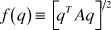 $$f{\kern 1pt} \left( q \right) \equiv \left[ {q^T Aq} \right]^{{1 \mathord{\left/ {\vphantom {1 2}} \right. \kern-\nulldelimiterspace} 2}} $$
where A ≡ [a ij] is an N by N symmetric matrix that has one positive eigenvalue (that has a strictly positive eigenvector) and the remaining N−1 eigenvalues are zero or negative. Under these conditions, there will be a region of regularity where the function f is positive, concave, and increasing, and, hence, f can provide a valid representation of preferences over this region. Using these preferences and the assumption of cost-minimizing behavior in periods 0 and 1, it can be shown that
 $$Q_F {\kern 1pt} \left( {p^0 ,{\kern 1pt} p^1 ,{\kern 1pt} q^0 ,{\kern 1pt} q^1 } \right) = {{f{\kern 1pt} \left( {q^1 } \right)} \mathord{\left/ {\vphantom {{f{\kern 1pt} \left( {q^1 } \right)} {f{\kern 1pt} \left( {q^0 } \right)}}} \right. \kern-\nulldelimiterspace} {f{\kern 1pt} \left( {q^0 } \right)}}.$$
Thus, under the assumption that the consumer engages in cost-minimizing behavior during periods 0 and 1 and has preferences over the N commodities that correspond to the utility function f defined by (45), the Fisher ideal quantity index Q F is exactly equal to the true quantity index, f(q 1)/f(q 0).Footnote 64
Let c(p) be the unit cost function that corresponds to the homogeneous quadratic utility function f defined by (45). Then, using (5), (42), and (46), it can be shown that
 $$P_F {\kern 1pt} \left( {p^0 ,{\kern 1pt} p^1 ,{\kern 1pt} q^0 ,{\kern 1pt} q^1 } \right) = {{c{\kern 1pt} \left( {p^1 } \right)} \mathord{\left/ {\vphantom {{c{\kern 1pt} \left( {p^1 } \right)} {c{\kern 1pt} \left( {p^0 } \right)}}} \right. \kern-\nulldelimiterspace} {c{\kern 1pt} \left( {p^0 } \right)}}.$$
Thus, under the assumption that the consumer engages in cost-minimizing behavior during periods 0 and 1 and has preferences over the N commodities that correspond to the utility function f(q) = (q TAq)1/2, the Fisher ideal price index P F is exactly equal to the true price index, c(p 1)/c(p 0). The significance of (46) and (47) is that we can calculate the consumer’s true rate of utility growth and his or her true rate of price inflation without having to undertake any econometric estimation; i.e., the left-hand sides of (46) and (47) can be calculated exactly using observable price and quantity data for the consumer for the two periods under consideration. Thus, the present economic approach to index number theory using a ratio approach leads to practical solutions to the index number problem, whereas the earlier levels approach explained in section II did not lead to practical solutions.
A twice continuously differentiable function f(q) of N variables q can provide a second order approximation to another such function f *(q) around the point q* if the level and all of the first and second order partial derivatives of the two functions coincide at q*. It can be shownFootnote 65 that the homogeneous quadratic function f can provide a second order approximation to an arbitrary f* around any point q* in the class of twice continuously differentiable linearly homogeneous functions. Thus, the homogeneous quadratic functional form defined by (45) is a flexible functional form.Footnote 66 Diewert (1976, pp. 117) termed an index number formula Q F(p 0, p 1, q 0, q 1) that was exactly equal to the true quantity index f(q 1)/f(q 0) (where f is a flexible functional form) a superlative index number formula.Footnote 67Equation (46) and the fact that the homogeneous quadratic function f defined by (45) is a flexible functional form shows that the Fisher ideal quantity index Q F is a superlative index number formula. Since the Fisher ideal price index P F also satisfies (47) where c(p) is the dual unit cost function that is generated by the homogeneous quadratic utility function, P F is also a superlative index number formula.
It is possible to show that the Fisher ideal price index is a superlative index number formula by a different route. Instead of starting with the assumption that the consumer’s utility function is the homogeneous quadratic function defined by (45), we could start with the assumption that the consumer’s unit cost function is a homogeneous quadratic. Thus, suppose that the consumer has the following unit cost function:
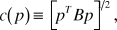 $$c{\kern 1pt} \left( p \right) \equiv \left[ {p^T Bp} \right]^{{1 \mathord{\left/ {\vphantom {1 2}} \right. \kern-\nulldelimiterspace} 2}} ,$$
where B ≡ [b ij] is an N by N symmetric matrix that has one positive eigenvalue (with a strictly positive eigenvector) and the remaining N−1 eigenvalues are zero or negative. It can be shown that again (47) holds. Thus, under the assumption that the consumer engages in cost-minimizing behavior during periods 0 and 1 and has preferences over the N commodities that correspond to the unit cost function defined by (48), the Fisher ideal price index P F is exactly equal to the true price index, c(p 1)/c(p 0).Footnote 68
Since the homogeneous quadratic unit cost function c(p) defined by (48) is also a flexible functional form, the fact that the Fisher ideal price index P F exactly equals the true price index c(p 1)/c(p 0) means that P F is a superlative index number formula.
It turns out that there are many other superlative index number formulae; i.e., there exist many quantity indexes Q(p 0, p 1, q 0, q 1) that are exactly equal to f(q 1)/f(q 0) and many price indexes P(p 0, p 1, q 0, q 1) that are exactly equal to c(p 1)/c(p 0) where the aggregator function f or the unit cost function c is a flexible functional form. We will define a family of superlative indexes below.
Suppose that the consumer has the following quadratic mean of order r utility function Footnote 69:
 $$f^r {\kern 1pt} \left( {q_1 , \ldots ,q_N } \right) \equiv \left[ {\sum\nolimits_{i = 1}^N {\sum\nolimits_{k = 1}^N {a_{ik} \,q_i^{r2} \,q_k^{{r \mathord{\left/ {\vphantom {r 2}} \right. \kern-\nulldelimiterspace} 2}} } } } \right]^{{1 \mathord{\left/ {\vphantom {1 r}} \right. \kern-\nulldelimiterspace} r}} $$
where the parameters a ik satisfy the symmetry conditions a ik = a ki for all i and k, and the parameter r satisfies the restriction r ≠ 0. Diewert (1976, pp. 130) showed that the utility function f r defined by (49) is a flexible functional form; i.e., it can approximate an arbitrary twice continuously differentiable linearly homogeneous functional form to the second order.Footnote 70 Note that when r = 2, f r equals the homogeneous quadratic function defined by (45) above.
Define the quadratic mean of order r quantity index Q r by:
 $$Q^r {\kern 1pt} \left( {p^0 ,{\kern 1pt} p^1 ,{\kern 1pt} q^0 ,{\kern 1pt} q^1 } \right) \equiv \left\{ {\sum\nolimits_{i = 1}^N {s_i^0 \left( {{{q_i^1 } \mathord{\left/ {\vphantom {{q_i^1 } {q_i^0 }}} \right. \kern-\nulldelimiterspace} {q_i^0 }}} \right)^{{r \mathord{\left/ {\vphantom {r 2}} \right. \kern-\nulldelimiterspace} 2}} } } \right\}^{{1 \mathord{\left/ {\vphantom {1 r}} \right. \kern-\nulldelimiterspace} r}} \left\{ {\sum\nolimits_{i = 1}^N {s_i^1 \left( {{{q_i^1 } \mathord{\left/ {\vphantom {{q_i^1 } {q_i^0 }}} \right. \kern-\nulldelimiterspace} {q_i^0 }}} \right)^{{{ - r} \mathord{\left/ {\vphantom {{ - r} 2}} \right. \kern-\nulldelimiterspace} 2}} } } \right\}^{{{ - 1} \mathord{\left/ {\vphantom {{ - 1} r}} \right. \kern-\nulldelimiterspace} r}} $$
where  $s_i^t \equiv {{p_i^t q_i^t } \mathord{\left/ {\vphantom {{p_i^t q_i^t } {\sum\nolimits_{k = 1}^N {p_k^t q_k^t } }}} \right. \kern-\nulldelimiterspace} {\sum\nolimits_{k = 1}^N {p_k^t q_k^t } }}$ is the period t expenditure share for commodity i. It can be verified that when r = 2, Q r simplifies to Q F, the Fisher ideal quantity index. It can be shown that Q r is exact for the aggregator function f r defined by (49); i.e., we have
 $$Q^r {\kern 1pt} \left( {p^0 ,{\kern 1pt} p^1 ,{\kern 1pt} q^0 ,{\kern 1pt} q^1 } \right) = {{f^r {\kern 1pt} \left( {q^1 } \right)} \mathord{\left/ {\vphantom {{f^r {\kern 1pt} \left( {q^1 } \right)} {f{\kern 1pt} \left( {q^0 } \right)}}} \right. \kern-\nulldelimiterspace} {f{\kern 1pt} \left( {q^0 } \right)}}.$$
Thus, under the assumption that the consumer engages in cost-minimizing behavior during periods 0 and 1 and has preferences over the N commodities that correspond to the utility function defined by (49), the quadratic mean of order r quantity index Q F is exactly equal to the true quantity index, f r(q 1)/f r(q 0).Footnote 71
Since Q r is exact for f r and f r is a flexible functional form, we see that the quadratic mean of order r quantity index Q r is a superlative index for each r ≠ 0. Thus, there are an infinite number of superlative quantity indexes.
For each quantity index Q r, we can use (5) in order to define the corresponding implicit quadratic mean of order r price index P r:
 $$P^r {\kern 1pt} \left( {p^0 ,{\kern 1pt} p^1 ,{\kern 1pt} q^0 ,{\kern 1pt} q^1 } \right) \equiv {{p^1 \, \cdot {\kern 1pt} q^1 } \mathord{\left/ {\vphantom {{p^1 \, \cdot {\kern 1pt} q^1 } {\left[ {p^0 \, \cdot {\kern 1pt} q^0 Q^r {\kern 1pt} \left( {p^0 ,{\kern 1pt} p^1 ,{\kern 1pt} q^0 ,{\kern 1pt} q^1 } \right)} \right]}}} \right. \kern-\nulldelimiterspace} {\left[ {p^0 \, \cdot {\kern 1pt} q^0 Q^r {\kern 1pt} \left( {p^0 ,{\kern 1pt} p^1 ,{\kern 1pt} q^0 ,{\kern 1pt} q^1 } \right)} \right]}} = {{c^r {\kern 1pt} \left( {p^1 } \right)} \mathord{\left/ {\vphantom {{c^r {\kern 1pt} \left( {p^1 } \right)} {c^r {\kern 1pt} \left( {p^0 } \right)}}} \right. \kern-\nulldelimiterspace} {c^r {\kern 1pt} \left( {p^0 } \right)}}$$
where c r is the unit cost function that is dual to the aggregator function f r defined by (49) above. For each r ≠ 0, the implicit quadratic mean of order r price index P r is also a superlative index.
When r = 2, Q r defined by (50) simplifies to Q F, the Fisher ideal quantity index and P r defined by (52) simplifies to P F, the Fisher ideal price index. When r = 1, Q r defined by (50) simplifies to
 $$Q^1 {\kern 1pt} \left( {p^0 ,{\kern 1pt} p^1 ,{\kern 1pt} q^0 ,{\kern 1pt} q^1 } \right) = {{\left[ {{{p^1 \, \cdot {\kern 1pt} q^1 } \mathord{\left/ {\vphantom {{p^1 \, \cdot {\kern 1pt} q^1 } {p^0 \, \cdot {\kern 1pt} q^0 }}} \right. \kern-\nulldelimiterspace} {p^0 \, \cdot {\kern 1pt} q^0 }}} \right]} \mathord{\left/ {\vphantom {{\left[ {{{p^1 \, \cdot {\kern 1pt} q^1 } \mathord{\left/ {\vphantom {{p^1 \, \cdot {\kern 1pt} q^1 } {p^0 \, \cdot {\kern 1pt} q^0 }}} \right. \kern-\nulldelimiterspace} {p^0 \, \cdot {\kern 1pt} q^0 }}} \right]} {P_W {\kern 1pt} \left( {p^0 ,{\kern 1pt} p^1 ,{\kern 1pt} q^0 ,{\kern 1pt} q^1 } \right)}}} \right. \kern-\nulldelimiterspace} {P_W {\kern 1pt} \left( {p^0 ,{\kern 1pt} p^1 ,{\kern 1pt} q^0 ,{\kern 1pt} q^1 } \right)}}\,$$
where P W is the Walsh (1901, p. 398; 1921a, p. 97) price index defined earlier by (13). Thus, the Walsh price index is also a superlative price index.
The above results provide reasonably strong justifications for the Fisher and Walsh price indexes from the viewpoint of the economic approach. An even stronger justificationFootnote 72 can be provided for the Törnqvist Theil index P T defined by (19), as we will show below.
Suppose that the consumer’s cost function, C(u, p), has the following translog functional form Footnote 73:
 $$\displaylines{ lnC{\kern 1pt} \left( {u,p} \right) \equiv a_0 + \sum\nolimits_{i = 1}^N {a_i \,lnp_i + \left( {{1 \mathord{\left/ {\vphantom {1 2}} \right. \kern-\nulldelimiterspace} 2}} \right)} \cr \sum\nolimits_{i = 1}^N {\sum\nolimits_{k = 1}^N {a_{ik} \,lnp_i \,lnp_k + b_0 \,lnu + \sum\nolimits_{i = 1}^N {b_i \,lnp_i \,lnu + \left( {{1 \mathord{\left/ {\vphantom {1 2}} \right. \kern-\nulldelimiterspace} 2}} \right)\;b_{00} \left[ {lnu} \right]^2 } } } \cr} $$
where ln is the natural logarithm function and the parameters a i, a ik, and b i satisfy the following restrictions: (i) a ik = a ki for i, k = 1,…, N; (ii)  $\sum\nolimits_{i = 1}^N {a_i = 1}$; (iii)
 $\sum\nolimits_{i = 1}^N {b_i = 0}$; and (iv)
 $\sum\nolimits_{k = 1}^N {a_{ik} = 0}$ for i = 1,…,N. These restrictions ensure that C(u,p) defined by (54) is linearly homogeneous in p. It can be shown that this translog cost function can provide a second order Taylor series approximation to an arbitrary cost function.Footnote 74
We assume that the consumer engages in cost-minimizing behavior during periods 0 and 1 and has the preferences that are dual to the translog cost function defined by (54). Define the geometric average of the period 0 and 1 utility levels as u* ≡ [u 0u 1]1/2. Then it can be shown that the log of P T defined by (19) is exactly equal to the log of the Konüs true cost of living index that corresponds to the reference indifference surface that is indexed by the intermediate utility level u *; i.e., we have the following exact identityFootnote 75:
 $${{C\left( {u^ * ,{\kern 1pt} p^1 } \right)} \mathord{\left/ {\vphantom {{C\left( {u^ * ,{\kern 1pt} p^1 } \right)} {C\left( {u^ * ,{\kern 1pt} p^0 } \right)}}} \right. \kern-\nulldelimiterspace} {C\left( {u^ * ,{\kern 1pt} p^0 } \right)}} = P_T {\kern 1pt} \left( {p^0 ,{\kern 1pt} p^1 ,{\kern 1pt} q^0 ,{\kern 1pt} q^1 } \right).$$
Since the translog cost function is a flexible functional form, the Törnqvist-Theil price index P T is also a superlative index.Footnote 76 The importance of (55) as compared to the earlier exact index number results is that it is no longer necessary to assume that preferences are homothetic. However, it is necessary to choose a particular utility level on the left-hand side of (55) to be the geometric mean of u 0 and u 1 in order to obtain the new exact index number result.Footnote 77
It is somewhat mysterious how a ratio of unobservable cost functions of the form appearing on the left-hand side of the above equation can be exactly estimated by an observable index number formula, but the key to this mystery is the assumption of cost-minimizing behavior and the quadratic nature of the underlying preferences. In fact, all the exact index number results derived in this section can be derived using transformations of a quadratic identity.Footnote 78
The important message to take home from this section is that the Fisher, Walsh, and Theil indexes, P F, P W,and P T, can all be given strong justifications from the viewpoint of the economic approach to index number theory. Note that these same formulae also emerged as being “best” from the viewpoints of the basket, stochastic, and test approaches to index number theory. Thus, the four major approaches to bilateral index number theory lead to the same three formulae as being best. Which formula should then be used by a statistical agency as their target index? It turns out that for “typical” time series data, it will not matter much, since the three indexes numerically approximate each other very closely.Footnote 79
The fact that four rather different approaches to index number theory lead to the same small number of index number formulae as being “best” and the fact that these formulae closely approximate each other for annual time series data has been a positive development. Twenty years ago, measurement economists and price statisticians from North America tended to favor the economic approach to index number theory, whereas their counterparts in Europe tended to favor the testFootnote 80 or stochastic approaches. This difference in views led to a great deal of counterproductive discussion on the relative merits of the various approaches to index number theory at international meetings on price measurement. Since, for all practical purposes, the various approaches lead to the same small number of index number formulae as being “best,” recent international meetings have been far more productive, with participants focused on how to improve price measurement rather than fighting methodological wars.
VII. FISHER ON THE STOCHASTIC AND ECONOMIC APPROACHES TO INDEX NUMBER THEORY
As we have seen above, Fisher made significant contributions to the test approach to index number theory but he did not contribute to the stochastic and economic approaches to index number theory because he was opposed to them.
Fisher (1922, p. 43) followed Walsh (1901; 1921a, pp. 82–83) in objecting to Edgeworth’s (Reference Edgeworth1888, Reference Edgeworth1896, Reference Edgeworth1901) unweighted stochastic approach explained in section IV above due to the lack of weighting in the Carli and Jevons indexes defined earlier by (16) and (18). Edgeworth also advocated taking the median of the price ratios  $\left( {{{p_n^1 } \mathord{\left/ {\vphantom {{p_n^1 } {p_n^0 }}} \right. \kern-\nulldelimiterspace} {p_n^0 }}} \right)$ as an easy-to-calculate index that would fit in well with his approach.Footnote 81 Fisher (1922, pp. 249–250) classified the median formula and the Jevons index as poor and the Carli index as worthless; i.e., for his data set, they gave numerical results that were rather far from the results generated by his ideal index P F.
Fisher was well aware of consumer theory but he rejected the economic approach to index number theory on the grounds that it was not practicalFootnote 82:
In this connection it may be well to call attention to another standard of purchasing power of money which has sometimes been suggested for adjusting contracts. This is the utility standard. According to this, each person would be expected to receive or pay back a marginal utility equivalent to what he had lent or borrowed. But the marginal utility of the same goods is different for different persons and different for the same person at different periods of his life. Hence, no such standard could be practically applied. (Fisher Reference Fisher1911, p. 220)
The development of the economic approach to price and quantity indexes had to wait until the path-breaking 1924 article of Konüs Reference Konüs(1924) was translated into English in Econometrica in 1939.Footnote 83
Thus, Fisher rejected the economic and stochastic approaches to index number theory (but he indirectly contributed to the stochastic approach by pointing out the upward bias in the Carli formula).
VIII. FISHER ON MULTILATERAL INDEXES AND FIXED BASE VERSUS CHAINED INDEX NUMBERS
As was noted in section VI above, Fisher (1911, p. 204) favored the use of chained index numbers but in Fisher (Reference Fisher1922), he favored direct comparisons between any two periods or, more generally, between any two spatial comparisons: “Similarly, turning from time to space, an index number for comparing the United States and England requires one set of weights, and an index number for comparing the United States and France requires, theoretically at least, another” (Fisher Reference Fisher1922, p. 275).
Thus, Fisher broadened the scope of index number theory to include spatial comparisons between countries or regions as well as the usual time series comparisons that were considered up to that time. The second point to note about Fisher’s Reference Fisher1922 position on index number comparisons is that when index number comparisons are made between N price and quantity situations, instead of computing N−1 indexes between the N points, we would have to compute N(N−1)/2 indexes; i.e., a matrix of bilateral comparisons would be required:
It follows that, to secure the theoretically most perfect result, for the sake of finding the very best for each pair of years, we should, for a given series of years and with a given formula, work out every possible index number connecting every possible pair of years among all the years considered. (Fisher Reference Fisher1922, p. 297)
Fisher (1922, p. 298) went on to note that we could compute a sequence of indexes where each time period or country would be the base, so for N price quantity situations, we could calculate N separate sequences of index number comparisons. In Fisher’s case, he had six observations and so six separate series could be generated using each year as the base. But there will be a demand for a single series of index number comparisons rather than six separate comparisons, so what should be done? Fisher had a very modern answer: “Doubtless the very best as to accuracy, were it practicable, is the blend or average of all six. This blend constitutes Formula 7053” (Fisher Reference Fisher1922, p. 305).
Thus, each of Fisher’s six series using each year as the base in turn was normalized to equal 1 in the first period, and then his best blend was the simple arithmetic average of these six normalized series. Fisher’s blended method is almost equal to Gini’s (Reference Gini1931) method except that Gini took the geometric mean of the six series rather than the arithmetic mean. Gini’s method is still widely used in making international comparisons.Footnote 84 Thus, Fisher was a pioneer in this area.
On the narrower issue of using fixed base versus chained indexes in the context of making time series comparisons, the modern literature has suggested that countries (or time periods) that have the most similar structure of prices and quantities should be linked, because with similar structures, the functional form for the bilateral index number formula will not matter too much: all “reasonable” indexes will generate much the same answer. A practical problem with this similarity linking approach is: exactly how should the measure of price or quantity similarity be measured?Footnote 85 For annual time series data, it turns out that for various “reasonable” similarity measures, chained indexes are generally consistent with the similarity approach to linking observations.
Fisher (1922, p. 309) found that for his data set, the six sets of index numbers that used each year as the base in turn were so close to the chained index numbers that the seven sets of price index comparisons could not be graphically distinguished. Thus, for his data set, the Fisher ideal index satisfied the circularity test to a high degree of approximation. Moreover, the time series generated by the Theil and Walsh indexes, P T and P W, were also very close to the fixed base and chained Fisher indexes. It is possible to give a theoretical explanation for these empirical results. Alterman, Diewert, and Feenstra (1999, p. 61) showed that if the logarithmic price ratios  $ln{\kern 1pt} \left( {{{p_n^t } \mathord{\left/ {\vphantom {{p_n^t } {p_n^{t - 1} }}} \right. \kern-\nulldelimiterspace} {p_n^{t - 1} }}} \right)$ trend linearly with time t and the expenditure shares
 $s_n^t$ also trend linearly with time, then the Törnqvist Theil index P T will satisfy the circularity test exactly.Footnote 86 Since many economic time series on prices and quantities satisfy these assumptions approximately, then the Törnqvist Theil index P T will satisfy the circularity test approximately. But Diewert (1978, p. 888) showed that P T, P F, and P W numerically approximate each other to the second order around an equal price and quantity point, and so these indexes will generally be very close to each other using annual time series data. Hence, since P T will generally satisfy the circularity test to some degree of approximation, P F will also satisfy circularity approximately in the time series context. Thus, for many economic time series, P F, P T, and P W will all satisfy the circularity test to a high enough degree of approximation so that it will not matter whether we use the fixed base or chain principle.
However, the situation changes if we are comparing countries or using sub annual time series data. In these cases, price and quantity vectors may be very different across observations, and so the smooth trend assumptions that justified the exact satisfaction of the circularity test for P T will not be satisfied. Under these conditions, chained indexes can give very unsatisfactory results; i.e., Walsh’s multiperiod identity test will be far from being satisfied. Under these conditions, fixed base indexes or multilateral methods will have to be used.Footnote 87
IX. CONCLUSION
It can be seen from the above material that Fisher contributed substantially to all the main approaches to bilateral index number theory that are in use today, except that he did not contribute to the economic approach. Fisher and Walsh are the early fathers of the test approach to index number theory. In addition, Fisher made substantial contributions to the modern theory of multilateral indexes. Fisher’s ideal index turns out to be a “best” formula from the viewpoint of the fixed basket, test, and economic approaches to index number theory. Finally, the Fisher ideal quantity index is being used as a target index when constructing estimates of real GDP by national statistical agencies such as the US Bureau of Economic Analysis. Fisher has left a lasting legacy to index number theory.