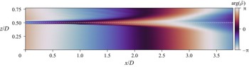
1. Introduction
Supersonic jets are complex flows exhibiting a variety of interactions between strong shock waves, small- and large-scale turbulent structures, internal modes and externally propagating acoustic waves. A particular example is found in under-expanded supersonic jets where such complex interactions can generate an aero-acoustic feedback mechanism known as screech (Powell Reference Powell1953), locking the jet dynamics into different possible modes or limit cycles. The complexity of the mechanisms involved has prevented the development of accurate prediction tools and experimental studies are still needed to better understand the main 3-D dynamics of these jets.
However, this complex environment poses metrological challenges. One promising way to address the problem is to consider seedless optical techniques for probing the jet density field. Among the different approaches that have been proposed in the literature, one of the optically simplest technique is tomographic background oriented schlieren (BOS) (Atcheson et al. Reference Atcheson, Ihrke, Heidrich, Tevs, Bradley, Magnor and Seidel2008; Nicolas et al. Reference Nicolas, Todoroff, Plyer, Le Besnerais, Donjat, Micheli, Champagnat, Cornic and Le Sant2016), which has been successfully applied to the study of supersonic jets by Nicolas et al. (Reference Nicolas, Donjat, Léon, Besnerais, Champagnat and Micheli2017) using a multi-camera set-up. Tomographic BOS can nevertheless be limited in terms of spatial resolution because the cameras are focused on the background and not on the flow of interest, but also because of spatial filtering induced by image correlation algorithms. Another optical technique used by Panda & Seasholtz (Reference Panda and Seasholtz1999) to provide density measurements in under-expanded jets is Rayleigh scattering. This technique offers fine spatial measurement resolution with significant accuracy. However, the measurement is pointwise, which is not ideal for the analysis of 3-D coherent structures, and the results can be particularly sensitive to Mie scattering.
The present work investigates the use of synchronised multi-axis digital holographic interferometry (DHI) for the study of the average and dynamical state of an under-expanded screeching supersonic jet in helical mode. This approach provides multiple dense observations of the flow at different angles as in tomographic BOS, but with a finer spatial resolution. It is then demonstrated how these flow projections can be leveraged to expose and analyse the main 3-D coherent structures associated with the observed helical instability.
1.1. Multi-view DHI
Applied to transparent media, holographic interferometry (HI) provides a means of evaluating the phase variations of an optical wavefront passing through a field of non-homogeneous refractive index in comparison with a reference state (Schnars et al. Reference Schnars, Falldorf, Watson and Jüptner2014; Picart, Gross & Marquet Reference Picart, Gross and Marquet2015). HI is then a line-of-sight technique that provides integral projections of a flow field and satisfactory estimation of an instantaneous 3-D density field thus requires simultaneous multi-directional acquisitions.
In the context of non-homogeneous 3-D flows, this idea was first followed some 50 years ago, with early works described by Matulka & Collins (Reference Matulka and Collins1971) and Sweeney & Vest (Reference Sweeney and Vest1974). These authors demonstrated that several interferograms obtained from different viewing angles using holographic plates could be successfully processed to estimate asymmetric density fields by solving a set of equations involving fringe number functions. At the time, recording devices were mainly analogue and the evaluation of the fringe number functions yielded by the interfering holograms could only be performed visually, ultimately providing measurements with a reduced spatial resolution.
The rise of digital recording devices has naturally led to significant improvements in this technique. Early applications to flow visualisation were reported by Watt & Vest (Reference Watt and Vest1987) who used a digital camera to record the interferometric pattern obtained by illuminating a double-exposed holographic plate. Post-processing of the fringe pattern could then be performed numerically, thus providing accurate and well-resolved instantaneous maps of interferometric phase delays. Relying on this approach, Snyder & Hesselink (Reference Snyder and Hesselink1988) and Watt & Vest (Reference Watt and Vest1990) later performed tomographic reconstructions of instantaneous density fields induced by a helium jet using several viewing angles. Snyder & Hesselink (Reference Snyder and Hesselink1988) used 18 instantaneous interferograms distributed around the jet axis whereas Watt & Vest (Reference Watt and Vest1990) relied on two orthogonal holographic plates from which multi-angular views of the holographic interferograms could be retrieved a posteriori with different camera orientations. At the time, this approach was already termed digital HI for the interferograms were digitised. It is noted however that, nowadays, DHI rather refers to the direct acquisition of digital holograms by a camera, with no need for a holographic plate (Schnars et al. Reference Schnars, Falldorf, Watson and Jüptner2014). Consequently, in this work, DHI will refer only to this recent definition, whereas the older approach will be referred to as ‘digitised HI’.
Tomographic digitised HI was further considered by Timmerman & Watt (Reference Timmerman and Watt1995) and Timmerman, Watt & Bryanston-Cross (Reference Timmerman, Watt and Bryanston-Cross1999) to study supersonic jets, relying on the initial single-view optical set-up proposed by Lanen, Bakker & Bryanston-Cross (Reference Lanen, Bakker and Bryanston-Cross1992). A digitised tomographic holographic interferometer was designed to simultaneously record on a single holographic plate six to nine different holograms of the flow of interest using a pulsed laser. A phase-stepping approach was used to unambiguously determine phase maps associated with the digitised interferograms and tomographic reconstruction was performed relying on an algebraic reconstruction method.
Interestingly, at about the same time, another tomographic interferometric technique was considered by Söller et al. (Reference Söller, Wenskus, Middendorf, Meier and Obermeier1994) and Dillmann, Wetzel & Soeller (Reference Dillmann, Wetzel and Soeller1998) to study supersonic jets. These authors relied on a single-view Mach–Zehnder interferometer set to an infinite fringe mode (Smits Reference Smits2012) to estimate phase variations from the interferograms. No holographic plate was required because the interferograms could be directly imaged on the camera sensor. Only one viewing angle was considered with this set-up and tomographic reconstructions were performed on mean flows, assuming flow axisymmetry.
This digital interferometric approach shares strong similarities with the holographic interferometric technique previously discussed because they both yield an interferometric pattern containing information about phase variations across the flow field. Yet, the holographic approach can be considered less stringent on the constraints applying to the optical path of the reference beam (Smits Reference Smits2012). Indeed, the double exposure technique in the holographic method ensures that the phase variations observed are exactly the ones induced by the flow itself, whereas in the case of interferometry the optical path of the reference beam is of prime importance. Nevertheless, this technical difference vanishes if one considers a Mach–Zehnder interferometer used in a finite fringe mode and if fringe patterns are made to interfere with a reference state acquired without flow. This exactly corresponds to DHI, where holograms are acquired by cameras (Schnars et al. Reference Schnars, Falldorf, Watson and Jüptner2014). This approach was recently followed and detailed by Sugawara et al. (Reference Sugawara, Nakao, Miyazato, Ishino and Miki2020) who also studied the mean structure of supersonic under-expanded jets. In the latter work, a single view was considered and tomographic reconstructions were again obtained assuming axisymmetry, relying on the inverse Abel transform. Single-view DHI with Abel transform has also been recently applied by Rodrigues et al. (Reference Rodrigues, Brown, Meyer and Lucht2022) to study under-expanded supersonic jets, but using high-speed cameras in an attempt to resolve temporal fluctuations in optical phase. Finally, Doleček et al. (Reference Doleček, Psota, Lédl, Vít, Václavík and Kopecký2013) and Doleček et al. (Reference Doleček, Psota, Lédl and Vít2016) studied heated synthetic jets using a single-axis DHI set-up and relied on a phase-averaging technique to acquire holograms of the periodic flow at different viewing angles. Tomographic reconstructions were then obtained by these authors relying on a classical inverse Radon transform.
This fully digital approach to holographic interferometry is nowadays possible due to the increased resolution of imaging sensors and the reduction in pixel size. The holograms are then directly acquired by high-definition camera sensors and the final interference phase maps can be retrieved by simple spectral post-processing. These technical refinements therefore now offer the opportunity to revisit multi-view holographic interferometry, in a way that shares similarities with the recently developed tomographic BOS technique, and to benefit from significant improvements made in tomographic reconstruction. Based on this idea, the first objective of this work is to detail in §§ 2 and 3 the development of a multi-axis DHI configuration adapted to the study of unsteady complex 3-D jet flows with large density gradients in a limited field of view.
1.2. Under-expanded screeching supersonic jets
The flow considered in this work is a round supersonic under-expanded jet issuing from a choked nozzle. Such a jet is obtained when a gas is exhausted through a contoured converging nozzle in an non-ideally expanded manner, i.e. when the flow static pressure at the exit,  $p_0$, is higher than the ambient pressure,
 $p_a$. The operating condition can then be defined by the nozzle pressure ratio
 $\text {NPR}= p_{t0}/p_a$ where
 $p_{t0}$ is the stagnation (or total) pressure at the nozzle exit. Equivalently, the ideally expanded Mach number
 $M_{j}$ can be used and is defined as
 \begin{equation} M_{j} = \left( \frac{2}{\gamma-1}\left[\text{NPR}^{{(\gamma-1)}/{\gamma}}-1\right] \right)^{{1}/{2}}, \end{equation}
where  $\gamma$ is the heat capacity ratio taken equal to
 $1.4$ for dry air.
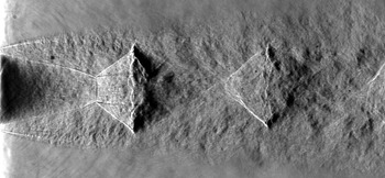
A detailed description of the average structure of under-expanded jets can be found in the review provided by Franquet et al. (Reference Franquet, Perrier, Gibout and Bruel2015). As illustrated by the schlieren visualisation shown in figure 1 for a jet at  $\text {NPR}{}=5$, under-expanded jets feature quasi-periodic shock-cell structures generated by successive expansion and compression waves trapped in the jet plume. For such a value of
 $\text {NPR}{}$, the Mach disc induced by a Mach reflection on the centreline is particularly visible in the first cell. The average structure of this type of jet has been extensively studied in the literature using such schlieren photographs, giving easy access to geometric parameters such as the average spacing of the shock cells and the diameter of the Mach disc.
Spark schlieren visualisation of an under-expanded supersonic jet at  $\text {NPR}{}=5$ and a total temperature of 293 K.

One particular aspect of under-expanded jets is the possible generation of an aeroacoustic feedback loop, inducing an extremely tonal screech noise (Raman Reference Raman1999; Edgington-Mitchell Reference Edgington-Mitchell2019). The basic understanding of this phenomenon is that the natural instability waves of the jet outer shear layer interact with the shock cells to produce upstream-travelling free-stream acoustic or internally guided waves that excite the jet shear layer at the nozzle lip (Edgington-Mitchell et al. Reference Edgington-Mitchell, Jaunet, Jordan, Towne, Soria and Honnery2018; Gojon, Bogey & Mihaescu Reference Gojon, Bogey and Mihaescu2018; Nogueira et al. Reference Nogueira, Jaunet, Mancinelli, Jordan and Edgington-Mitchell2022), which is a high-receptivity region of the jet. This resonant closed-loop mechanism then amplifies the most unstable waves, providing a highly frequency-selective mechanism that may be understood as a global instability (Edgington-Mitchell et al. Reference Edgington-Mitchell, Wang, Nogueira, Schmidt, Jaunet, Duke, Jordan and Towne2021; Nogueira et al. Reference Nogueira, Jordan, Jaunet, Cavalieri, Towne and Edgington-Mitchell2021). Interestingly, different frequencies are selected when varying the  $\text {NPR}{}$ and sharp frequency jumps are usually observed, permitting the identification of different screech modes. Following the terminology proposed by Powell (Reference Powell1953), the four main modes are labeled A, B, C and D. Each mode was reported by Powell, Umeda & Ishii (Reference Powell, Umeda and Ishii1992) to present different azimuthal structures, that were deduced to be mainly axisymmetric, flapping, helicoidal and flapping with rotation, respectively. A variety of measurement techniques have been used to study these modes, with schlieren visualisations and acoustic measurements being the most common (see, for example, André, Castelain & Bailly Reference André, Castelain and Bailly2011). Density fields, however, are more rarely studied: among the few references, Panda & Seasholtz (Reference Panda and Seasholtz1999) relied on Rayleigh scattering to obtain pointwise measurements whereas Nicolas et al. (Reference Nicolas, Donjat, Léon, Besnerais, Champagnat and Micheli2017) and Lanzillotta et al. (Reference Lanzillotta, Léon, Donjat and Le Besnerais2019) used tomographic BOS to evidence the average spatial structure of two screech modes.
Overall, field measurements providing detailed quantitative descriptions of under- expanded screeching jets are relatively scarce in the literature, particularly when it comes to the structure of the jet over the first few nozzle diameters and the flow dynamics in the vicinity of the Mach disc. Notable work on this point was performed by Edgington-Mitchell, Honnery & Soria (Reference Edgington-Mitchell, Honnery and Soria2014a) who conducted a planar PIV experiment to describe the velocity field of an under-expanded jet in helical screech mode C, at  $\text {NPR}{}=4.2$, with a particular emphasis on the embedded annular shear layer present behind the first Mach disc. This work highlighted the influence of azimuthal large-scale structures developing in the external jet shear layer on the reflected shock, which was then hypothesised to force the internal annular jet shear layer in a coherent but out-of-phase manner. This dynamical link between the structures found in the outer and inner jet shear layers, and more generally between the main screech instability and inner jet motions, has not been experimentally reexamined to the knowledge of the present authors. Using the capability of the developed multi-view DHI set-up to access the azimuthal content of a density field, the second objective of the present work pursued in § 4 is to provide another quantitative look at the dynamical features occurring in screeching under-expanded jets in helical mode.
2. DHI and 3-D density field estimation
DHI being a line-of-sight technique, it naturally requires an appropriate inversion methodology to reconstruct 3-D density fields. Furthermore, the raw measurements provided by DHI are interferometric patterns that need to be converted to relative optical thicknesses or phase variations before tomographic processing. This section thus discusses the different physical notions required to understand the methodology followed to develop the present multi-view DHI set-up.
2.1. DHI for transparent media
Considering a 3-D flow field of refractive index  $n_\lambda (\boldsymbol {x})$ at a wavelength
 $\lambda$, a coherent wavefront passing through will be distorted, inducing variations in optical path lengths (OPLs, denoted
 $\varLambda$) compared with a reference situation without flow. The OPL of a monochromatic light ray following a path
 $C$ is defined as
 \begin{equation} \varLambda = \int_C n_\lambda(s) \,\mathrm{d}{s} , \end{equation}
where  $s$ is a curvilinear abscissa. The field of refractive index being related to the flow density field
 $\rho (\boldsymbol {x})$ by the Gladstone–Dale relation, this equation can be written as
 \begin{equation} \varLambda = \int_C \left( \mathcal{K}_\lambda \rho(s) + 1 \right) \,\mathrm{d}{s}, \end{equation}
where  $\mathcal {K}_\lambda$ refers to the Gladstone–Dale constant of the fluid at the considered wavelength
 $\lambda$. The variation of OPL
 $\delta \varLambda$ with respect to a reference flow situation with uniform density
 $\rho _0$ then writes
 \begin{equation} \delta\varLambda = \mathcal{K}_\lambda \int_C \left(\rho(s)-\rho_0\right) \,\mathrm{d}{s} . \end{equation}
The OPL variations may be related to phase variations  $\delta \phi$ in the initial wavefront using the dispersion relation, yielding
 \begin{equation} \delta\phi=2{\rm \pi} \frac{\delta\varLambda}{\lambda} . \end{equation}
DHI provides a way to measure these integrated phase variations  $\delta \phi$ by evaluating the phase difference of two digital holograms obtained for the two different flow states. This phase difference is equivalent to the interference phase obtained using an analogue holographic approach where these holograms are made to interfere by re-illumination. Details about the formation of holograms and their processing may be found in references such as Schnars et al. (Reference Schnars, Falldorf, Watson and Jüptner2014) or Picart et al. (Reference Picart, Gross and Marquet2015), and only the basics are reminded here. A hologram is the result of the interference of two light waves in an observation plane: a reference wave traversing a transparent medium that does not change over time and a second wave that passes through the unsteady transparent medium of interest. It can be noted that holographic techniques are most commonly used with opaque or translucent objects, but the physical principles remain the same. Assuming the use of a monochromatic light, the complex amplitude of the reference wavefront in the observation plane
 $(\eta, \xi )$ can be expressed as
 \begin{equation} E_{r}(\eta, \xi) = a_{r}(\eta, \xi)\,\exp\left[\mathrm{i} \phi_{r}(\eta, \xi)\right], \end{equation}
where  $a_{r}$ refers to the real amplitude,
 $\phi _{r}$ to the phase of the reference wave and
 $\mathrm {i}$ is the imaginary unit. Similarly, the measurement wavefront reaching the observation plane after traversing the transparent media (the object) and thus integrating the associated phase changes is written as
 \begin{equation} E_{o}(\eta, \xi) = a_{o}(\eta, \xi)\exp\left[\mathrm{i} \phi_{o}(\eta, \xi)\right], \end{equation}
where  $a_{o}$ and
 $\phi _{o}$ refer to the real amplitude and the phase of the measurement wave. These two waves interfere in the observation plane and the resulting light intensity captured by the camera sensor is given by
 \begin{align} I(\eta, \xi) & = |E_{r} + E_{o}|^{2} \end{align}
 \begin{align} & = \underbrace{|E_{r}|^{2} + |E_{o}|^{2}}_{0 \text{ order}} + \underbrace{E_{r}^{*}E_{o}}_{{+}1\text{ order}} + \underbrace{E_{r}E_{o}^{*}}_{{-}1\text{ order}}, \end{align}
where the superscript  ${\cdot }^{*}$ refers to the complex conjugate. Three diffraction order terms can be identified in this equation, terms that will be further discussed and illustrated in § 2.3. This expression can also be written as
 \begin{equation} I(\eta, \xi) = a_{r}^{2} + a_{o}^{2} + 2a_{r}a_{o}\cos(\phi_{o}-\phi_{r}) , \end{equation}
showing that the digital hologram is made of a background (the zero-order term), determined by the intensity of the two wavefronts, and an interference term varying with the phase difference  $\phi _{o}-\phi _{r}$. The interference pattern obtained depends on the direction of propagation of the two waves: in an ‘off-axis’ DHI set-up, i.e. when the two waves are made to propagate in slightly different directions, a spatial carrier wave is formed permitting efficient isolation of the phase difference term from the zero-order term as presented in § 2.3.
Post-processing the interferograms then allows the estimation of phase difference maps  $\Delta \phi (\eta, \xi )=\phi _{o}-\phi _{r}$ in the observation plane for one flow state. As a consequence, the phase difference
 $\delta \phi$ between two flow states, required to evaluate the OPL variations
 $\delta \varLambda$ using (2.4), can be simply estimated by the difference
 \begin{equation} \delta\phi(\eta, \xi) = \Delta \phi_{n} - \Delta \phi_{0}. \end{equation}
Here,  $\Delta \phi _{n}$ refers to the holographic phase of the flow of interest acquired at an instant
 $t_{n}$ and
 $\Delta \phi _{0}$ to a reference holographic phase, typically obtained without flow. As mentioned in the introduction, a clear advantage of this approach over traditional interferometric methods is that the estimated phase variation
 $\delta \phi$ does not depend on
 $\phi _{r}$, the phase of the reference wave, because it is cancelled in the subtraction process.
2.2. Mach–Zehnder interferometric set-up for DHI
Different optical set-ups may be considered to perform off-axis DHI with transparent media. As emphasised by Desse & Olchewsky (Reference Desse and Olchewsky2017), when studying flows with large density gradients one particularly needs to account for the sensitivity of the apparatus and possible shadow effects arising from light refraction. Indeed, the presence of shock waves in the flow was shown to cast shadows in the holograms, with a detrimental effect on phase estimation. This was particularly observed using a Michelson interferometer which relies on a double-pass of the measurement wave through the flow of interest. In contrast, with a Mach–Zehnder interferometer, the measurement wave only traverses the flow once. As a result, the sensitivity is halved, but shadow effects can be greatly reduced by properly focusing the imaging system on the flow. Based on this experimental result, a similar optical set-up is considered in the present work.
A classical set-up for off-axis DHI relying on a Mach–Zehnder interferometer is schematically illustrated in figure 2. The laser beam is split in two by a beamsplitter cube. The reference beam is spatially filtered ( $SF_2$), expanded and directed to a recombination cube (
 $L_4$,
 $M_2$). This reference wave traverses a quiescent atmosphere with uniform density and its path towards the recombination cube is controlled using a flat mirror (
 $M_2$). The angle
 $\theta$ of this mirror controls the direction of propagation of the reference wave relative to the measurement wave after recombination and its fine-tuning is necessary to generate a spatial carrier wave as discussed in § 2.1. The measurement wave is also filtered (
 $SF_1$) and expanded to traverse the measurement volume in parallel rays (
 $M_1$,
 $L_1$) before being reduced using an afocal optical set-up (
 $L_2$,
 $L_3$) and reaching the recombination cube. Both waves then illuminate the camera sensor to create a digital hologram, with the fringe spacing and orientation of the spatial carrier being controlled by
 $\theta$.
Schematic of a single-camera Mach–Zehnder interferometer used to perform off-axis DHI. Here  $M_{i}$ refers to flat mirrors,
 $L_{i}$ to spherical lenses and
 $SF_i$ to spatial filters.

A practical implementation of this Mach–Zehnder interferometer for the analysis of a supersonic jet will be presented in § 3. At this stage, some important constraints associated with this optical set-up can be emphasised. First, the size of the volume of interest is limited by the size of the spherical lenses  $L_1$ and
 $L_2$, usually limiting the technique to flows a few centimeters wide. Second, the laser source needs to produce a light with sufficient coherence length to ensure proper formation of an interferometric pattern on the camera sensor during exposure time. For high-speed flows such as that investigated in this work and for which short-time illumination is required to obtained instantaneous snapshot holograms of the flow, specific pulsed lasers with long coherence length are then needed. Finally, vibrations in the optical system can be particularly detrimental to the measurement and care must be taken to reduce them as much as possible. For example, it is necessary to ensure a certain level of steadiness in the density field traversed by the reference wave as well as an absence of temporal drifts that may be induced by such vibrations.
2.3. Interferograms processing
Once the digital holograms are acquired, phase maps need to be estimated. Two steps are required with the present approach: phase evaluation and phase map unwrapping.
2.3.1. Phase map evaluation
Two main approaches are usually considered to recover the phase distribution  $\Delta \phi$ from the interferometric image associated with (2.7): temporal phase-stepping (or phase-shifting) and spectral filtering (Picart et al. Reference Picart, Gross and Marquet2015). The latter method is considered in the present work since a reference state (without flow) can be easily acquired, permitting phase estimation with a single acquisition and enabling the analysis of instantaneous density distributions in high-speed flows with an optical set-up of reduced complexity.
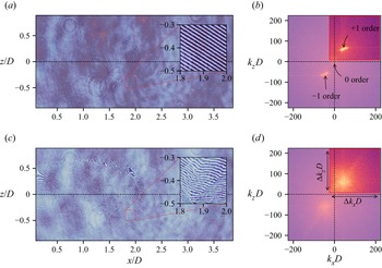
The main idea of this technique is to isolate the  $+1$ diffraction order from (2.8) and to evaluate its phase. This is possible in off-axis DHI because of the use of a spatial carrier frequency yielding a clear separation of the different diffraction orders in Fourier space. For example, figure 3(a) displays an interferogram acquired in a reference state, i.e. without flow, with the apparatus later described in § 3. In this figure, the
 $(x,z)$ coordinate system used is deduced from that of the observation plane
 $(\eta,\xi )$ by application of the optical magnification factor of the apparatus, with an origin located at the centre of the jet exit plane. An inset highlights the fringe pattern induced by the off-axis modulation and its chosen orientation which is approximately at
 $45^{\circ }$. The amplitude of the 2-D Fourier transform of this image is represented in figure 3(b), using a logarithmic scale. The different diffraction orders are easily identified and can thus be individually filtered, as originally proposed by Takeda, Ina & Kobayashi (Reference Takeda, Ina and Kobayashi1982) in a different context.
Examples of (a,c) digital holograms in the aerodynamic plane  $(x,z)$ and (b,d) associated 2-D spectra obtained respectively without flow (reference state) and with an under-expanded supersonic jet (
 $\text {NPR}=5$) in the measurement beam using the experimental set-up described in § 3. In (a,c), the insets provide local magnifications on the fringe patterns. In (b,d), a logarithmic scale on the spectrum amplitude was used and the parts of the spectra that are filtered out are coloured using lighter tones. Here
 $k_i$ refers to a wavenumber in the
 $i$th direction and
 $D$ is the diameter of the jet nozzle exit.

Different spectral filter shapes and functions may be considered. In this work, the pupil of the optical set-up was verified to produce an Airy pattern smaller than the pixel size of the camera, thus such that no selection limitation in the Fourier spectrum appears. A classical rectangular filter was then chosen since it provided consistent results for all the cases considered. After application of this filter and inverse Fourier transform, a filtered hologram  $I_{F}$ isolating the
 $+1$ diffraction order is obtained, writing
 \begin{equation} I_{F}(\eta,\xi) = \mathcal{F}^{{-}1}\left(W(k_{\eta}, k_{\xi})\, \mathcal{F}(I)\right) , \end{equation}
where  $\mathcal {F}$ refers to Fourier transform and
 $W(k_{\eta }, k_{\xi })$ is the filtering window in the wavenumber plane. An example of such a filtering is given in figure 3(b), where the red rectangle indicates the bounds of the chosen filter. The zero order is concentrated at the origin and the selected window discards this region while retaining about a quarter of the 2-D spectrum. This window was furthermore chosen to isolate the
 $+1$ diffraction order for the cases where the flow of interest was in the measurement beam. An example of interferometric pattern captured in this situation is shown in figure 3(c), highlighting the large changes in fringe orientation induced by the inhomogeneous density field. The associated 2-D spectrum is displayed in figure 3(d), where the previous filtering window is also shown. Compared with the reference state, the variations in the fringe pattern induce a spread of the spectral support of the
 $+1$ order, but the selected window still captures most of the associated content.
The holographic phase  $\Delta \phi$ is then deduced (modulo
 $2{\rm \pi} )$ from the filtered hologram
 $I_F$ by evaluating its argument, thus writing
 \begin{equation} \Delta \phi(\eta,\xi) = \arg(I_{F}(\eta,\xi)) . \end{equation}
Consequently, the phase difference in (2.10) can be estimated by applying this methodology to the reference hologram and to a hologram acquired with a given flow state. This phase difference, however, is only given modulo  $2{\rm \pi}$ because of (2.12), providing phase difference distributions
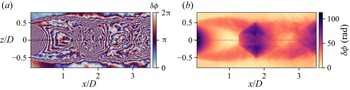
 $\delta \phi$ as illustrated in figure 4(a) which was obtained following this procedure for the two holograms shown in figure 3. In order to correctly estimate OPL variations for tomographic reconstruction, a phase-unwrapping procedure is required to restore continuous 2-D phase distributions.
(a) Folded phase difference map deduced from the digital holograms shown in figure 3 and (b) the corresponding map of unwrapped phase difference obtained using the algorithm proposed by Herraez et al. (Reference Herraez, Burton, Lalor and Gdeisat2002).

2.3.2. Phase unwrapping
Phase map unwrapping aims at restoring a folded phase distribution to its original continuous form, free of  $2{\rm \pi}$ jumps. This task can be relatively complex when dealing with noisy data such as holographic phase measurements. In the present case, an additional difficulty is brought by the presence of shock waves in the flow of interest, which naturally induce large phase jumps in some regions of the flow. Various strategies have been proposed in the literature to handle such difficulties (Ghiglia & Pritt Reference Ghiglia and Pritt1998). Among the different algorithms available, that proposed by Herraez et al. (Reference Herraez, Burton, Lalor and Gdeisat2002) was found to be particularly robust for unwrapping the present phase maps, generally correctly handling the large phase jumps associated with shocks and the phase measurement noise.
An example of application of this unfolding algorithm is shown in figure 4(b), where no obvious unwrapping aberrations can be observed and where phase values around shock waves present sharp transitions. It can be emphasised at this stage that the phase maps obtained provide differential values and that the external region of the flow is considered as the reference region. Consequently, phase maps are automatically adjusted by an additive constant to provide zero phase values on average in this region.
Finally, it should be highlighted that the overall measurement uncertainty of the phase difference  $\delta \phi$ obtained after demodulation, filtering and unwrapping is not straightforward to estimate. Future work will have to address this point which requires a dedicated study in itself and which is thus deliberately left aside. It can nonetheless be noted that phase measurement noise should be equal to or greater than the noise observed in the reference holograms, i.e. without flow. With the set-up detailed in § 3, it has been estimated to be approximately 0.15 rad.
2.4. Resolution
The Mach–Zehnder interferometric set-up presented in figure 2 ensures that the measurement wavefront is planar in the test section. The holographic image then spatially resolves the flow to the sensor resolution of the camera in the observation plane. However, the spectral filtering process previously discussed degrades the spatial resolution of this phase measurement (Picart et al. Reference Picart, Gross and Marquet2015). Indeed, (2.11) may be written as
 \begin{equation} I_F(\eta, \xi) = I(\eta,\xi) * w(\eta, \xi), \end{equation}
where  $*$ refers to the convolution operator and
 $w$ is the impulse response of the rectangular filter
 $W$ applied in the Fourier domain. This impulse response can be expressed in the following form in the observation plane,
 \begin{equation} w(\eta, \xi) = \Delta k_\eta \Delta k_\xi \text{sinc}(\Delta k_\eta \eta) \text{sinc}(\Delta k_\xi \xi) E, \end{equation}
where  $\text {sinc}$ refers to the normalised sinc function,
 $\Delta k_\eta$ and
 $\Delta k_\xi$ are the dimensions of the rectangular window
 $W$ in the wavenumber plane and
 $E= \exp ({\mathrm {i} (k_{\eta,0}\eta + k_{\xi,0}\xi )})$ with
 $(k_{\eta,0}, k_{\xi,0})$ the centre of the rectangular window. The sinc functions appearing in this kernel will thus spatially smooth the hologram whose resolution will then depend on
 $\Delta k_\eta$ and
 $\Delta k_\xi$. In the present work, the filter size generally covers a quarter of the 2-D spectrum as shown in figure 3 and the order of magnitude of the phase measurement spatial resolution in the observation plane is then approximately two pixels.
With the DHI optical set-up presented in § 3, given a magnification factor of  $0.12$, this leads to an estimated spatial resolution for phase measurements of approximately
 $100\,\mathrm {\mu }{\rm m}$. It is instructive to compare this value with those reported in studies relying on tomographic BOS to study similar flows: Nicolas et al. (Reference Nicolas, Donjat, Léon, Besnerais, Champagnat and Micheli2017) reported a measurement resolution in the displacement fields of approximately 2.5 mm and Lanzillotta et al. (Reference Lanzillotta, Léon, Donjat and Le Besnerais2019) improved the BOS optical set-up to achieve a spatial resolution of approximately 0.9 mm. The effect of such differences on the description of the flow was particularly discussed by Champagnat et al. (Reference Champagnat, Nicolas, Olchewsky, Donjat, Essaïdi and Desse2018). Although some improvements on these values can certainly be obtained, this discussion emphasises that DHI more naturally gives a high-resolution description of an object, which is particularly beneficial for the analysis of flows presenting large density variations as in the work of Sugawara et al. (Reference Sugawara, Nakao, Miyazato, Ishino and Miki2020). Clearly, this comes at a price of a more complex set-up that can only be used for flows of limited spatial extents.
2.5. Tomographic reconstruction
With the obtained maps of unwrapped phase difference  $\delta \phi$, the variations of OPL can be deduced using (2.4). It then remains to solve the inverse problem of estimating the density field
 $\rho (\boldsymbol {x})$ from a set of line integrals (2.3), obtained simultaneously at different projection angles. An important aspect of DHI is that the light rays probing the volume of interest are parallel, thus permitting the treatment of this tomographic reconstruction problem slice by slice along the jet axis, as in X-ray computed tomography. The projection operator to be considered thus corresponds to the well-known 2-D Radon transform. This is in contrast to BOS tomography (Nicolas et al. Reference Nicolas, Todoroff, Plyer, Le Besnerais, Donjat, Micheli, Champagnat, Cornic and Le Sant2016; Grauer et al. Reference Grauer, Unterberger, Rittler, Daun, Kempf and Mohri2018), where the entire volume must be considered in the inverse problem which involves 3-D light ray deviations, making the inference process more computationally challenging. (It can nonetheless be noted that when considering mean axisymmetric flows, dedicated approaches (Xiong, Kaufmann & Noiray Reference Xiong, Kaufmann and Noiray2020) such as the inverse Abel transform and its generalisation accounting for non-parallel light rays (Sipkens et al. Reference Sipkens, Grauer, Steinberg, Rogak and Kirchen2021) can be considered for BOS tomography at a reduced numerical cost.)
Considering a slice of the probed volume, a solution to this inverse problem is sought by discretising it on a cartesian grid with  $M\times M$ square elements of constant density. The discretised measurement model (2.3) in matrix form can then be expressed as
 \begin{equation} \boldsymbol{\mathsf{T}}_\theta \boldsymbol{\chi} = \boldsymbol{b}_\theta, \end{equation}
where matrix  $\boldsymbol{\mathsf{T}}_\theta \in \mathbb {R}^{M\times M^2}$ refers to the discrete projection operator performing integration along the paths followed by the light rays at the projection angle
 $\theta$,
 $\boldsymbol {\chi }= (\boldsymbol {\rho }-\rho _{0})\in \mathbb {R}^{M^2}$ is the 2-D field of density difference in the considered slice rearranged in a (uni-column) vector and
 $\boldsymbol {b}_\theta \in \mathbb {R}^{M}$ is the vector gathering the observed variations in optical phase at the observation angle
 $\theta$. Considering now
 $N_{\theta }$ projection angles
 $\{\theta _{i}\}_{[1..N_{\theta }]}$, the global linear inverse problem in matrix form may be written as
 \begin{equation} \boldsymbol{\mathsf{T}} \boldsymbol{\chi} = \boldsymbol{b} \end{equation}
with  $\boldsymbol{\mathsf{T}}\in \mathbb {R}^{MN_{\theta }\times M^2}$ and
 $\boldsymbol {b}\in \mathbb {R}^{MN_{\theta }}$, where the
 $N_{\theta }$ observed projections are stacked in a single vector. This vector
 $\boldsymbol {b}$ can be viewed as a flatten sinogram.
One major difficulty hindering a direct resolution of this problem is that  $\boldsymbol{\mathsf{T}}$ is ill-conditioned because of the sparsity of the projections (the lower the number of projections, the larger the condition number of
 $\boldsymbol{\mathsf{T}}$) and the smoothing action of the measurement process given by (2.3) implying that measurement noise naturally present in the projections can significantly corrupt the solution. Various strategies have been proposed in the literature to handle these problems. The two main families of reconstruction methods are the analytical (Fourier methods, filtered back-projection, etc.) and the regularised approaches. The latter are of interest in the context of this work for two main reasons: first, they provide a way to distill prior knowledge about the solution and, second, efficient solving methods have been proposed in the literature.
In a Bayesian framework, regularised methods provide maximum a posteriori (MAP) solutions in which a measurement noise model is naturally taken into account and where  $\boldsymbol {\chi }$ is considered as a random process. Formally, the problem amounts to solving
 \begin{equation} \underset{\boldsymbol{\chi}}{\text{argmin}}\left\{\mathcal{F}(\boldsymbol{\mathsf{T}} \boldsymbol{\chi}-\boldsymbol{b}) + \mu\, \mathcal{G}(\boldsymbol{\chi})\right\} \end{equation}
using an optimisation procedure. The first term of this compound criterion provides a measure of data fidelity assuming a measurement noise model while the second one is a regularisation term driving the solution under a priori physically-plausible constraints. Here,  $\mu$ is the regularisation parameter and
 $\mathcal {G}(\,\cdot\,)$ is a regularisation function. In the following, a least-squares data model is considered, such that
 $\mathcal {F}(\,\cdot \,)=\frac {1}{2}\|\cdot \|_2^2$. This corresponds to the assumption of a normally distributed measurement noise. This hypothesis has been validated based on the analysis of a series of unfolded reference interferograms and should be approximately valid for averaged phase measurements in the presence of flow. Indeed, unlike DHI applied to opaque surfaces, no speckle noise is present in the holograms. Regarding the regularisation term, various functions have been proposed in the literature depending on the type of problem to be solved. To enforce the smoothness of the solution, a Tikhonov (or
 $\ell _{2}$) regularisation approach (Tikhonov & Arsenin Reference Tikhonov and Arsenin1977) can be used, as chosen by Nicolas et al. (Reference Nicolas, Todoroff, Plyer, Le Besnerais, Donjat, Micheli, Champagnat, Cornic and Le Sant2016) for example for BOS tomography on hot jets and plumes. In the present study, however, a supersonic flow featuring shock waves and thus sharp density gradients is considered. As a consequence, an approach relying on (isotropic) total variation (TV) was selected instead to best capture discontinuities in the estimated solution, such that
 $\mathcal {G}(\,\cdot \,)=\text {TV}(\,\cdot \,)$.
As TV regularisation introduces a non-differentiable function, a different framework than the classical gradient descent approach in the optimisation procedure is required and can be found in proximal splitting methods (Chambolle & Pock Reference Chambolle and Pock2016). In the present work, this optimisation problem is solved relying on the fast iterative shrinkage-thresholding algorithm (FISTA) (Beck & Teboulle Reference Beck and Teboulle2009) with a primal–dual TV algorithm (Chambolle & Pock Reference Chambolle and Pock2010) for the regularisation problem. Such an approach can be easily followed using open-source codes such as ASTRA-Toolbox (van Aarle et al. Reference van Aarle, Palenstijn, Beenhouwer, Altantzis, Bals, Batenburg and Sijbers2015) and ToMoBAR (Kazantsev Reference Kazantsev2019).
The choice of the regularisation parameter  $\mu$ is performed using an L-curve method (Idier Reference Idier2010), where the regularisation term is plotted as a function of the data-fidelity term in log–log scales for various values of
 $\mu$. As discussed by Hansen (Reference Hansen2001) for
 $\ell _{2}$ regularisation problems, a satisfactory compromise may be expected for values of
 $\mu$ where a change of slope is observed in this graph, or equivalently, when the graph curvature
 $\kappa$ is maximum. While acknowledging that this simple heuristic approach may be limited in certain cases of study, it has been observed in the present work (where TV regularisation is used) that it provides satisfactory estimates of
 $\mu$ with a slight tendency to give under-regularised solutions. This heuristic approach has been used because the exact level of measurement noise is unknown, precluding the use of estimation methods based on the discrepancy principle for example (Hansen Reference Hansen1998). It can furthermore be underlined that the regularisation parameter
 $\mu$ will depend on the choice of regularisation function but also significantly on the amount of measurement noise.
Finally, this tomographic reconstruction process is probably the main source of uncertainty in the estimated density fields. The subject of uncertainty estimation in tomographic reconstruction is, however, very complex and not settled, requiring a dedicated study out of the scope of the present work. Therefore, no definite confidence intervals can be proposed. Nevertheless, given the results discussed in § 4.1.2, it is reasonable to expect that in the present work the uncertainty in the density estimates could be better than  ${\pm }5\,\%$ overall. This level of uncertainty is relatively arbitrary, however, and further work is needed to provide objective values.
3. Experimental set-up for multi-view DHI on a screeching supersonic jet
3.1. Under-expanded jet set-up
The jet facility used is similar to that described by Nicolas et al. (Reference Nicolas, Donjat, Léon, Besnerais, Champagnat and Micheli2017) and Lanzillotta et al. (Reference Lanzillotta, Léon, Donjat and Le Besnerais2019). As illustrated in figure 5, it comprises a contoured, converging nozzle with an inner diameter  $D=22\,{\rm mm}$. This nozzle shape ensures a choked condition at the exit. This flush-mounted nozzle is placed in the middle of a
 $400\,{\rm mm} \times 400\,{\rm mm}$ metallic panel, providing an extremely thick lip nozzle configuration. The exhausted air is regulated in mass-flow rate and total temperature, with the former maintained at
 $T_{t0} = 293\,{\rm K}$ throughout the experiments. The
 $\text {NPR}$ was monitored using a total pressure probe located
 $32-D$ upstream of the convergent nozzle. In the present work, only one aerodynamic condition given by
 $\text {NPR}{}=5$ is discussed. This value corresponds to an ideally expanded Mach number
 $M_{j}=1.71$ and provides a jet sustaining a helical screech mode C as reported by Lanzillotta et al. (Reference Lanzillotta, Léon, Donjat and Le Besnerais2019) with the present jet facility. Finally, the Reynolds number of the jet based on ideally expanded values is
 ${\textit {Re}}_{j}= U_{j}\rho _{j}D_{j}/\mu _{j}\approx 1.8\times 10^{6}$ with
 $\rho _{j}\approx 1.89\,{\rm kg}\,{\rm m}^{-3}$.
Schematic of the nozzle geometry issuing an under-expanded supersonic jet. The field of view observed by DHI is represented using a blue dashed circle that has an approximate diameter of  $4.5D$ where
 $D$ is the nozzle exit diameter.

3.2. Synchronised multi-view DHI set-up
The Mach–Zehnder interferometer presented in § 2.2 was designed taking into account the size of the flow of interest. As illustrated in figure 5, the measurement area extends over a few jet diameters. Given the available volume around the jet and the size and cost of the required optics, an optical set-up based on concave mirrors instead of spherical lenses was chosen. A schematic of this Mach–Zehnder interferometer is provided in figure 6, illustrating the paths of the reference and measurement waves. In this optical set-up, the concave mirrors have a diameter of 100 mm and a focal length of 1 m. A compact arrangement is obtained by folding the optical path of the measurement wave using flat mirrors between the beamsplitters and the concave mirrors. These concave mirrors are combined with spherical lenses to form two afocal systems. The one in front of the camera has a lens of 120 mm focal length, giving an imaging magnification factor of  $0.12$. This set-up was used to obtain the 2-D results previously presented in § 2.
Schematic of one DHI line used to study an under-expanded supersonic jet. In this Mach–Zehnder interferometer, the reference wave is depicted in red and the measurement beam is shown in blue. BS, beamsplitter; PH, pinhole; FM, flat mirror; CM, concave mirror.

A multi-view DHI set-up was then obtained by repeating this optical layout by rotational symmetry around the jet axis. As mentioned in § 2.5, the number of projections and their angular distribution are important for the accuracy of the tomographic reconstruction process. Studies on the effects induced by these parameters for tomographic BOS have been reported by Nicolas et al. (Reference Nicolas, Todoroff, Plyer, Le Besnerais, Donjat, Micheli, Champagnat, Cornic and Le Sant2016) and Lang et al. (Reference Lang, Oberleithner, Paschereit and Sieber2017). The conclusions drawn in these studies are expected to be relevant for the present work since closely related tomographic tools are used. The latter authors particularly highlighted the performance of reconstruction of an axisymmetric density field with cameras evenly distributed on a half-circle or on a full circle, for an even or odd number of projections. Of interest for the present work, it was shown that for such a simplified density field and for a reduced number of cameras (lower than eight), the best results were obtained with an odd number of cameras distributed on a full circle or with cameras distributed on a half-circle. Furthermore, as expected, the larger the number of projections, the more accurate the reconstructions, with a minimum number of projections around eight before reaching marginal improvements with a half-circle distribution.
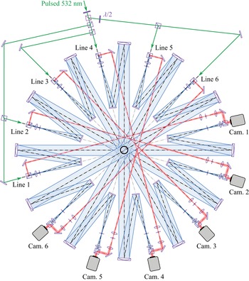
In the present work, the guidelines provided by these studies could not be followed because of the bulk of each Mach–Zehnder interferometer. Only six lines could be fitted around the jet on a half-circle, every  $30^{\circ }$, as depicted in figure 7. Such a number of projections is relatively small and artifacts limiting the accuracy of the reconstructed density fields are then generally to be expected with direct reconstructions, i.e. without providing additional prior knowledge about the flow topology. This is illustrated for example by Olchewsky et al. (Reference Olchewsky, Essaidi, Desse and Champagnat2018) with non-axisymmetric helium jets and
 $\ell _{2}$ regularisation. Nonetheless, this optical layout is perfectly suited to investigate the azimuthal structure of a flow mainly characterised by a reduced azimuthal wavenumber content because it offers a direct means to perform azimuthal Fourier decomposition of the observed projections. This approach is particularly leveraged in § 4 to study the main dynamical structure of the present under-expanded jet.
Schematic of the complete optical set-up used for multi-view DHI. This set-up is composed of six Mach–Zehnder interferometers similar to that displayed in figure 6, centred on the nozzle exit and arranged every  $30^{\circ }$.

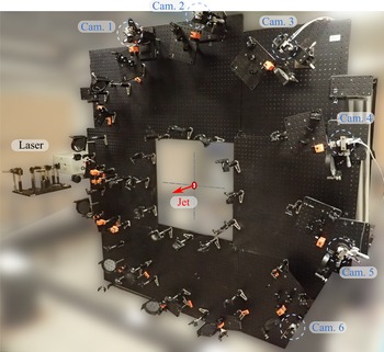
The practical realisation of this multi-view DHI set-up is shown in figure 8. Once built horizontally on optical boards, it was re-assembled vertically around the jet nozzle exit on four pneumatic isolators to reduce system vibration. The laser source used was a pulsed Nd:YAG laser (Quanta-Ray Lab-170-10, Spectra Physics) lasing at  $\lambda =532\,{\rm nm}$ and equipped with an injection seeder, providing a coherence length of approximately 3 m and enhanced output energy stability. It was triggered using a pulsed generator also synchronising the cameras at a frequency of 10 Hz. In order to balance the amount of energy distributed in each holographic line, the laser beam was successively divided using polarised splitter cubes as shown in figure 7. It can be noted here that this azimuthally distributed optical layout resembles that designed by Ishino et al. (Reference Ishino, Hayashi, Razak, Kato, Kurimoto and Saiki2015) to quantitatively study the 3-D structure of premixed turbulent flames using 20 synchronised projections. However, these authors relied on schlieren visualisation lines that are simpler to set-up than DHI lines but that also arguably provide less-accurate quantitative measurements.
Photograph of the multi-view DHI set-up vertically installed around the panel issuing the under-expanded jet.

3.3. Holograms recording
The digital holograms were recorded using a set of six digital cameras (Basler ace U) equipped with a  $1920\,{\rm px} \times 1200\,{\rm px}$ CMOS sensor with pixel size of
 $5.86\,\mathrm {\mu }{\rm m}$. Before performing acquisition at the selected
 $\text {NPR}{}$, a series of reference holograms was recorded without flow. Then, three series of
 $300$ digital holograms of the jet were acquired by each camera synchronised on the laser trigger signal at 10 Hz, with continuous operation of the jet facility. Therefore, a total of
 $900$ holograms were obtained for each DHI line.
4. Results and analysis
The optical phase measurements obtained by the multi-view DHI set-up on an under-expanded jet at  $\text {NPR}{}=5$ are analysed in the following sections. First, the average optical phase and density fields are presented in § 4.1. Then, the main coherent structures associated with the measured optical phase variations are extracted by azimuthal Fourier decomposition and snapshot proper orthogonal decomposition (POD) in § 4.2.
4.1. Mean density reconstruction
4.1.1. Mean optical phase map
The jet flow being axisymmetric, the map of mean optical phase  $\overline {\delta \phi }$ is evaluated by ensemble and azimuthal averaging of 854 instantaneous maps acquired with the six holographic lines. This operation thus provides the mean zeroth-order azimuthal Fourier mode. The number of instantaneous optical phase maps considered is slightly reduced compared with the total number of acquired snapshots since some outliers for which the optical phase maps were not correctly unwrapped were discarded.
The resulting map is displayed in figure 9(a). In this figure, three particular axial locations are highlighted. First, the Mach disc is estimated to be located around  $x=1.34D$. This value is in agreement with estimates reported by Addy (Reference Addy1981) and Nicolas et al. (Reference Nicolas, Donjat, Léon, Besnerais, Champagnat and Micheli2017) for a contoured converging nozzle. Similarly, a matching estimate of
 $0.35D$ for the Mach disc diameter is obtained. Second, the axial locations of the tips of the first two shock cells are evaluated to be around
 $1.83-D$ and
 $3.63-D$, providing a shock-cell spacing of approximately
 $1.8D$. Again, this estimate is consistent with the value generally obtained with choked jets at such a pressure ratio (Davies & Oldfield Reference Davies and Oldfield1962; Powell Reference Powell2010). The mean structure of the present choked under-expanded jet thus appears to be consistent with results reported in the literature.
(a) Map of mean unwrapped optical phase  $\overline {\delta \phi }$ measured on a choked under-expanded jet at
 $\text {NPR}{}=5$ using the multi-view DHI set-up and (b) the mean density ratio
 $\bar {\rho }/\rho _{a}$ deduced by axisymmetric tomographic reconstruction, with
 $\rho _{a}$ the density of the quiescent atmosphere.

4.1.2. Mean density field
By construction, the mean optical phase map in figure 9(a) displays perfect reflection symmetry across the horizontal axis. As shown in figure 9(b), tomographic reconstruction of the associated density field using the methodology outlined in § 2.5 was then performed accordingly, assuming exact axisymmetry. This is achieved by considering slices of mean optical phase  $\overline {\delta \phi }$ at all axial locations
 $x/D$ as input data for the tomographic process where it was chosen to use 64 repeated projections evenly distributed on half a circle. It can be noted that a more conventional approach relying on the inverse Abel transform could have been used for this task, as performed by Sugawara et al. (Reference Sugawara, Nakao, Miyazato, Ishino and Miki2020) for example. However, as emphasised subsequently, the purpose here is to provide validation results for the present tomographic methodology and to discuss the advantages of relying on a regularised tomographic approach.
A suitable value for the regularisation parameter  $\mu$ in (2.17) is required for satisfactory density field reconstructions. The L-curve plots and the corresponding (log–log) graph curvature plots
 $\kappa (\mu )$ obtained for three different slices are displayed in figures 10(a) and 10(b), respectively. These L-curves give clear graph curvature maxima that are obtained for similar values of
 $\mu$. As a consequence, a single value
 $\mu =5\times 10^{-5}$ was considered for final reconstruction of the mean density field.
(a) L-curves  $\log (\|\boldsymbol {\chi }\|_\text {TV})=f(\log (\|\boldsymbol{\mathsf{T}}\boldsymbol {\chi }-\boldsymbol {b}\|_{2}))$ obtained at three axial locations
 $x/D\in \{1,2,3\}$ for a logarithmically varying regularisation parameter
 $\mu$ in the reconstruction process of the mean density field
 $\bar {\rho }$. (b) The corresponding (log–log) graph curvature curves
 $\kappa (\mu )$ with
 $\kappa = f^{\prime \prime }/(1+f^{\prime 2})^{3/2}$.

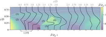
A longitudinal cross-section of the reconstructed density field ratio  $\bar {\rho }/\rho _a$ is shown in figure 9(b) and mean relative density profiles
 $(\bar {\rho }-\rho _{a})/\rho _{a}$ in this
 $(xz)$-plane are given in figure 11. The mean density field being axisymmetric, its 3-D structure can be easily pictured, particularly up to the first shock cell which appears to be very stable in time. Following the discussion provided by Panda & Seasholtz (Reference Panda and Seasholtz1999) for similar jets, different flow regions have been highlighted in figure 11 using dashed grey lines. The first line labeled (1) indicates approximately the curved boundary of the jet above which one finds the outer mixing layer. Line (2) indicates the presence of a weak shock generated by the coalescence of compression waves. This weak shock delimits the expansion region in the jet core and is known as the barrel shock or the intercepting shock. This expansion ends with a normal shock wave, before which the density falls well below the ambient one, forming the Mach disc identified by (4). From the point of intersection of the Mach disc and the barrel shock (known as the triple point) emanates a reflected shock labeled (3) and an embedded shear layer (5) which delimits a subsonic region downstream of the Mach disc and a supersonic flow region downstream of the reflected shock wave (3). As expected, a density larger than the ambient density (and than
 $\rho _{j}$) is found between this slip stream (5) and the reflected shock (3). The reflected shock (3) then intersects the external shear layer, giving rise to an expansion fan (6) which closes the first shock cell. Further downstream, a second expansion thus appears leading to a second, more diffuse shock cell. The structure of this density field and the density levels found appear to be in satisfactory agreement with the measurements obtained by Panda & Seasholtz (Reference Panda and Seasholtz1999) using Rayleigh scattering for jets at slightly lower and higher Mach numbers, i.e.
 $M_{j}=1.6$ and
 $1.8$, respectively.
Solid line: Radial profiles of mean relative density ratio  $\bar {\rho }/\rho _{a}-1$ obtained by axisymmetric tomographic reconstruction at various axial locations
 $x/D$ overlayed on the map of mean density ratio shown in figure 9(b). Here
 $\rho _{a}$ refers to the ambient density. Each density profile has its origin horizontally shifted to coincide with the axial location of the slice in the mean density map displayed in the background. The scale of these profiles is given by the double-headed arrow along the
 $x$-axis. For conversion purpose,
 $\rho _{j}/\rho _{a}\approx 1.55$. The white dotted lines provide iso-contours of
 $\bar {\rho }/\rho _{a}-1$ at a level of
 $0.05$.

As displayed in figure 11, the density profiles are slightly staggered, which is a direct consequence of the use of TV regularisation because it promotes solutions for which  $\boldsymbol {\nabla } \boldsymbol {\rho }$ is sparse. Although it can then be expected that the resulting density levels are not perfectly accurate, this drawback is compensated by a satisfactory capture of density jumps across the shock waves present in the flow. In particular, it can be highlighted that a sharp density jump across the reflected shock (3) is captured (see figure 11,
 $x/D=1.5$). It is interesting to note that, for comparison, Sugawara et al. (Reference Sugawara, Nakao, Miyazato, Ishino and Miki2020) did not retrieve such a feature in their case of study, probably because of their reconstruction process based on inverse Abel transform. Similarly, sharper density jumps across the embedded annular shear layer are obtained with a progressive thickening in the streamwise direction. As observed in figures 9(b) and 11, a second advantage over other tomographic reconstruction approaches is the absence of numerical artifacts in regions of uniform density such as the external region of the jet or within its core.
Finally, a quantitative comparison of the mean density ratio  $\bar {\rho }/\rho _{j}$ estimated along the jet axis with other measurements reported in the literature is provided in figure 12. The present DHI results are displayed with a
 $\pm 5\,\%$ band to quantitatively illustrate the data dispersion associated with such an arbitrary but plausible uncertainty level. First, compared with tomographic BOS results obtained by Nicolas et al. (Reference Nicolas, Donjat, Léon, Besnerais, Champagnat and Micheli2017), similar density levels are observed but with a better capture of the density profile across the Mach disc. Indeed, tomographic BOS results probably suffer from a larger spatial resolution associated with the BOS optical set-up and a more complex tomographic reconstruction process relying on a
 $\ell _{2}$ regularisation which probably oversmooths the gradients. Second, compared with the density profile obtained by Panda & Seasholtz (Reference Panda and Seasholtz1999) at a higher Mach number
 $M_{j}=1.8$ (
 $\text {NPR}{}\approx 5.75$), a very similar shape is obtained, supporting the relevance of the reconstructed field. In the present case, the location of the Mach disc is closer to the jet exit plane and larger density levels (close to
 $\rho _{j}$) in the shock-cell regions are measured. This is expected because the higher the Mach number, the greater the excessive heating due to non-isentropic compression associated with the normal shock wave and thus the lower the density in these regions. Finally, it can be highlighted that the density profile measured after the first Mach disc is relatively flat, showing a plateau value over an extent in the streamwise direction corresponding to the internal subsonic region delimited by the embedded axisymmetric shear layer (from
 $x/D\approx 1.34$ to
 $x/D\approx 2$). A slightly different behaviour is observed in the second shock cell, with a progressive increase in density (
 $x/D\approx 3.5$), in agreement with the measurements reported by Panda & Seasholtz (Reference Panda and Seasholtz1999).
Mean density ratio  $\bar {\rho }/\rho _{j}$ along the jet axis at
 $\text {NPR}{}=5$ (
 $M_{j}=1.71$) obtained with the present experimental apparatus (DHI) and with tomographic BOS (Nicolas et al. Reference Nicolas, Donjat, Léon, Besnerais, Champagnat and Micheli2017), with
 $\rho _{j}$ the fully expanded isentropic jet density. The axial profile measured by Panda & Seasholtz (Reference Panda and Seasholtz1999) using Rayleigh scattering at
 $M_{j}=1.8$ is also given for qualitative comparison purpose. The isentropic value at the nozzle exit is given by a red circle.

4.2. Identification of the main coherent structures
Whereas the previous mean-field analysis mainly focused on axisymmetric results for which only a single holographic line could have been used, a methodology exploiting the simultaneity of the acquisitions obtained with the six holographic lines is now discussed, with the objective of identifying the main coherent azimuthal structure of the fluctuating density field.
4.2.1. Phase fluctuation map
An instantaneous optical phase distribution obtained with one holographic line can be decomposed into a mean component  $\overline {\delta \phi }$, discussed in the previous § 4.1, and a fluctuating component
 $\widetilde {\delta \phi }$, such that
 \begin{equation} \delta\phi(t, \eta, \xi, \theta_{k}) = \overline{\delta\phi}(\eta, \xi, \theta_{k}) + \widetilde{\delta\phi}(t, \eta, \xi, \theta_{k}) , \end{equation}
where  $t$ refers to a discrete time,
 $(\eta, \xi )$ to the coordinates in the observation space and
 $\theta _{k}$ to the
 $k$th projection angle. Similarly, an instantaneous 3-D density field
 $\rho$ is decomposed into a mean field
 $\bar {\rho }$ and a fluctuating field
 $\tilde {\rho }$, writing
 \begin{equation} \rho(t, x, y, z) = \bar{\rho}(x, y, z) + \tilde{\rho}(t, x, y, z) , \end{equation}
where  $(x, y, z)$ are the coordinates in physical space. By linearity of the operators in (2.3) and (2.4), the two optical phase terms
 $\overline {\delta \phi }$ and
 $\widetilde {\delta \phi }$ are the projected results at an angle
 $\theta _k$ of
 $\bar {\rho }$ and
 $\tilde {\rho }$, respectively. Analysing the statistical properties of
 $\widetilde {\delta \phi }$ thus provides information on the structure of
 $\tilde {\rho }$.
The azimuthally averaged field of root mean square (r.m.s.) values of  $\widetilde {\delta \phi }$, referred to as
 $\delta \phi ^{\prime }$, is shown in figure 13 and highlights the projected regions of the flow with intense density variations. The reflected shock wave in the first shock cell appears to sustain some local but intense fluctuations, particularly at the junction with the external shear layer. Downstream, significant fluctuations in the jet shear layer and in the second shock cell can also be observed, as well as in the embedded shear layers to a lesser extent. Finally, this figure shows the well-known presence of a spatially stationary wave envelope outside the jet shear layer, which is the interfering result of downstream and upstream propagating waves that are building blocks in the screech feedback mechanism (Panda & Seasholtz Reference Panda and Seasholtz1999; Edgington-Mitchell Reference Edgington-Mitchell2019). The resulting wave is generally referred to as the jet near-field ‘standing wave’.
Map of root mean square values of temporal optical phase fluctuations  $\delta \phi ^{\prime }= \text {r.m.s.}(\widetilde {\delta \phi })$.

4.2.2. Azimuthal structure of the observed projections
As emphasised previously, the six-view DHI set-up was designed to provide instantaneous optical phase maps with observation lines regularly distributed in the jet azimuthal direction, for projection angles  $\theta _k\in \{0^{\circ }, 30^{\circ },\ldots, 150^{\circ }\}$. As the observed optical phases result from integration through the entire flow field, an augmented observation state for the optical phase fluctuations can be constructed by rotational symmetry around the jet axis, such that
 \begin{gather} \widetilde{\delta\phi}^a(t, \eta, \xi, \theta_k) = \widetilde{\delta\phi}(t, \eta, \xi, \theta_k), \end{gather}
 \begin{gather}\widetilde{\delta\phi}^a(t, \eta, \xi, \theta_k + 180^{{\circ}}) = \widetilde{\delta\phi}(t, \eta, -\xi, \theta_k) . \end{gather}
This augmented observation state is then defined for projection angles homogeneously distributed all around the jet, every  $30^{\circ }$, and can be decomposed into azimuthal Fourier modes
 $\hat {\delta \phi }^a_{m}$ with azimuthal wavenumbers
 $m\in \{-N_{\theta },\ldots, N_{\theta }-1\}$, writing
 \begin{equation} \widetilde{\delta\phi}^a(t, \eta, \xi, \theta_k) = \frac{1}{2N_\theta} \sum_{m={-}N_{\theta}}^{N_{\theta}-1}\hat{\delta\phi}^a_{m}(t, \eta, \xi) \mathrm{e}^{\mathrm{i}m\theta_k} , \end{equation}
where  $N_\theta =6$ in the present study. The instantaneous and average azimuthal structure of optical phase fluctuations can then be obtained, providing insights into the azimuthal structure of the flow density field.
The azimuthal mean energy distribution of the optical phase fluctuations is assessed by considering mean square values of the azimuthal Fourier modes amplitudes  $|\hat {\delta \phi }^{a}_{m}|$. Indeed, time-averaging Parseval's relation allows to define a mean distribution of azimuthal optical phase fluctuation energy
 $\bar {E}_{\theta }(\eta, \xi )$ such that
 \begin{equation} \bar{E}_{\theta} = \sum_{k=0}^{2N_{\theta}-1} \text{var}(\widetilde{\delta\phi}^{a}(t, \theta_{k})) = \frac{1}{2N_{\theta}} \sum_{m={-}N_{\theta}}^{N_{\theta}-1}\langle|\hat{\delta\phi}^{a}_{m}(t)|^{2}\rangle , \end{equation}
where  $\langle\,\cdot \,\rangle$ refers to the ensemble mean,
 $\text {var}(\,\cdot \,)$ to the variance operator along the time dimension and where the coordinates in the observation space have been omitted for clarity. The maps of normalised values of
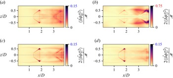
 $\langle |\hat {\delta \phi }^{a}_{m}(t)|^{2}\rangle$ are displayed in figures 14(a)–14(d) for four azimuthal wavenumbers, the remaining modes having low energy content. Relying on (4.6), the normalisation term used is
 $\mathcal {M}=\max (2N_{\theta }\bar {E}_{\theta })$, permitting the identification of regions in the azimuthal Fourier modes contributing the most to the observed optical phase fluctuations. It is emphasised that in these figures, the contributions of positive and negative azimuthal wavenumbers
 ${\pm }m$ are summed, resulting in a factor of two on the maps of non-axisymmetric modes (
 $m>0$) because
 $\hat {\delta \phi }^{a}_{\pm m}$ are complex conjugates. Figure 14(b) highlights that most of the optical phase fluctuations are associated with the
 $m=\pm 1$ helical modes, with local values reaching up to 75 % of the observed maximum mean optical phase fluctuation energy. These large fluctuations are identified in the region of the flow where the second shock cell interacts with the external jet shear layer. Significant fluctuations are also present upstream, in the outer shear layer found between the two shock cells and in the reflected shock of the first cell. As displayed in figures 14(a), 14(c) and 14(d), the other azimuthal modes have approximately five times smaller maximum fluctuation energy amplitudes. Interestingly, all of these azimuthal modes capture significant fluctuations in the oblique shock of the first shock cell, particularly in the region where it intersects the external shear layer. This suggests that shock oscillation in the first shock cell cannot be explained primarily by the dynamics of a single pair of azimuthal modes, in contrast to the second shock cell whose motion appears to be largely driven by the first helical modes
 $m=\pm 1$.
Maps of relative energy distribution in the first four azimuthal Fourier modes of observed optical phase fluctuations: (a)  $m = 0$, (b)
 $m = {\pm }1$, (c)
 $m = {\pm }2$ and (d)
 $m = {\pm }3$. For clarity only, the aerodynamic frame is used instead of the observation one. The normalisation term is
 $\mathcal {M}=\max (2N_\theta \bar {E}_\theta )$, see (4.6). As emphasised using coloured labels, (b) displays maximum values five times larger compared with (a), (c) and (d).

The dominance of the first pair of helical modes is made more evident in figure 15 which provides a measure of the relative magnitudes of the total energy contained in the maps  $\langle |\hat {\delta \phi }^{a}_{m}|^{2}\rangle$ using the Frobenius norm denoted by
 $\|\,\cdot \,\|_{F}$. Although the first pair of helical modes at
 $m=\pm 1$ provides approximately 58 % of the total energy, the other azimuthal modes all have contributions of less than 10 %.
Relative magnitudes of phase fluctuation energy contained in the 2-D maps of mean square azimuthal Fourier modes amplitudes  $\langle |\hat {\delta \phi }^{a}_{m}|^{2}\rangle$ as a function of the azimuthal wavenumber
 $m$, with summed contributions for complex conjugate pairs.

Finally, the map of r.m.s. values of optical phase fluctuations  $\delta \phi ^{\prime }$ previously shown in figure 13 is decomposed in figures 16(a) and 16(b) by isolating and discarding the contributions of the first pair of helical modes, respectively. As observed in figure 16(a), the dominant pair of azimuthal modes at
 $m=\pm 1$ captures the footprint of the standing wave present in the external near-field of the jet, this feature being almost totally absent from the map associated with the remaining modes in figure 16(b). As previously stated, this standing wave can be associated with the screech feedback loop. This observation, along with the large optical phase fluctuations observed, suggest that the salient features of screech mode C characterised by a helical instability wave are captured by the present azimuthally filtered measurements.
Maps of r.m.s. values of temporal optical phase fluctuations  $\delta \phi ^{\prime }$ obtained (a) by isolating the contributions of the first pair of complex-conjugate azimuthal modes (
 $m=\pm 1$) and (b) by considering the contributions of all the other azimuthal modes (
 $m\neq \pm 1$).

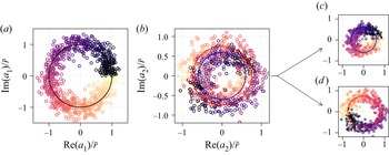
4.2.3. POD of the dominant helical Fourier mode
The previous azimuthal Fourier decomposition provided insights into the time-average azimuthal energy distribution of the observed optical phase fluctuations, highlighting that screech-related dynamical structures were embedded in the isolated complex-conjugate modes at  $m=\pm 1$. Yet, because of the unsteady nature of the system, which is furthermore only observed at discrete and distant time intervals, exposing an average 3-D density picture of these structures is not straightforward.
In this work, it is proposed to rely on POD (Holmes et al. Reference Holmes, Lumley, Berkooz and Rowley2012) to efficiently isolate these coherent structures and to provide a simple modelling framework for their dynamics. POD aims at decomposing an ensemble of space–time-varying fields  $\{f(t_{j}, \boldsymbol {x})\}_{j=1..P}$ into a linear combination of spatial orthogonal modes
 $\varPsi _{i}^{(f)}(\boldsymbol {x})$ optimally capturing its temporal variance or energy. Here,
 $\boldsymbol {x}\in \mathbb {R}^{3}$ refers to spatial coordinates in the frame of interest, which can be in the physical or in the observation space. It is emphasised that
 $f$ is considered in this work as a zero-mean complex-valued function and that, consequently, the spatial modes are also complex. The decomposition writes
 \begin{equation} f(t_{j}, \boldsymbol{x}) = \sum_{i=1}^{P}a_{i}(t_{j})\varPsi_{i}^{(f)}(\boldsymbol{x}) , \end{equation}
with  $a_{i}(t_{j})$ the discrete temporal complex coefficients animating the spatial modes. In discrete form, data functions and spatial modes are replaced by
 $N_{xyz}$-vectors, with
 $N_{xyz}$ the number of spatial points considered, such that (4.7) may be written as
 \begin{equation} \boldsymbol{f}_{j} = \sum_{i=1}^{P}a_{i,j}\boldsymbol{\varPsi}_{i}^{(f)} . \end{equation}
Following Sirovich (Reference Sirovich1987), when the observations  $\{\boldsymbol {f}_{j}\}$ are independent, this decomposition can be retrieved by considering the eigenvalue problem associated with the
 $P\times P$ temporal covariance matrix
 $\boldsymbol{\mathsf{C}}^{(f)}$ defined by elements
 $c^{(f)}_{m,n}=\boldsymbol {f}_{n}^{\operatorname {H}} \boldsymbol {f}_{m}/P$ where
 ${\cdot }^{\operatorname {H}}$ refers to the conjugate transpose operator. The eigenvectors of
 $\boldsymbol{\mathsf{C}}^{(f)}$ provide the temporal coefficients
 $a_{i,j}$ and the spatial modes are obtained by linear combination, such that
 \begin{equation} \boldsymbol{\varPsi}_{i}^{(f)} = \sum_{j=1}^{P} a_{i,j} \boldsymbol{f}_{j} . \end{equation}
Furthermore,  $\boldsymbol{\mathsf{C}}^{(f)}$ being Hermitian, its eigenvalues
 $\lambda _{i}$ are real and give the energy associated with the spatial modes
 $\boldsymbol {\varPsi }_{i}^{(f)}$. This approach is computationally interesting when
 $P\ll N_{xyz}$ and is commonly referred to as the method of snapshots.
In this work, the  $P$ augmented snapshots of optical phase
 $\widetilde {\delta \phi }^{a}$ are arranged as
 $QN_{\theta }^{a}$-dimensional vectors and stacked in a matrix
 $\boldsymbol {\varPhi }\in \mathbb {R}^{QN_{\theta }^{a}\times P}$, with
 $Q=MN_{x}$ the number of data points in one phase map and
 $N^{a}_{\theta }=2N_{\theta }$ the number of augmented projections. Snapshot POD is then applied to the deduced
 $P$ maps of helical Fourier modes at
 $m=1$ arranged as
 $Q$-dimensional vectors and stacked to form the snapshot matrix of Fourier modes
 $\hat {\boldsymbol {\varPhi }}_{m=1}\in \mathbb {C}^{Q\times P}$. The temporal covariance matrix can then be written
 $\boldsymbol{\mathsf{C}}^{(\phi )}=\hat {\boldsymbol {\varPhi }}_{m}^{\operatorname {H}}\hat {\boldsymbol {\varPhi }}_{m}/P$. Solving the associated eigenproblem provides the real eigenvalues
 $\lambda _{i}$ and the associated POD modes
 $\hat {\boldsymbol {\varPsi }}_{i}^{(\phi )}\in \mathbb {C}^{Q}$ for
 $i\in [1..P]$, which can be rearranged to form complex spatial maps of size
 $M\times N_{x}$. Selecting a limited number of main modes, an inverse discrete azimuthal Fourier transform may then be applied to obtain an arbitrary number
 $N^{\prime }_{\theta }>N_{\theta }$ of projections in the observation space of optical phase fluctuations, thus allowing an accurate reconstruction of the associated density fields to be performed relying on the tomographic reconstruction approach described in § 2.5.
This way of proceeding to estimate the density field of screech-related spatio-temporal modes is summarised in the flowchart shown in figure 17 using solid black arrows, where azimuthal Fourier transform and snapshot POD are directly performed on the entire set of observations. Other paths may however be imagined and it is important to clarify whether the present process yields main modes similar to those that would be obtained with azimuthal Fourier transform and POD directly applied to snapshots of density fields. Indeed, such an approach may be considered more physically relevant because the decomposition would then be performed in physical space and not in observation space. This way of proceeding is also illustrated in the flowchart shown in figure 17, but using dashed grey arrows. First, the inverse tomographic problem for the ensemble of acquired projections would have to be solved, providing the matrix  $\boldsymbol{\mathsf{X}}\in \mathbb {R}^{N_{xyz}\times P}$ gathering the
 $P$ temporal snapshots of 3-D fields of
 $\tilde {\rho }$ obtained on a Cartesian grid of size
 $N_{xyz}=N_x M^{2}$. An azimuthal Fourier transform would then directly provide the azimuthal Fourier modes
 $\widehat {\boldsymbol{\mathsf{X}}}_{m}$ and the deduced covariance matrix would be
 $\boldsymbol{\mathsf{C}}^{(\rho )}=\widehat {\boldsymbol{\mathsf{X}}}_{m}^{\operatorname {H}}\widehat {\boldsymbol{\mathsf{X}}}_{m}/P$. Applying an inverse Fourier transform to the selected main POD modes would finally provide the main 3-D structures of density fluctuations associated with screech. Clearly, the major drawback with this approach lies in its first step, because it requires tomographic inversion of the entire set of projections. In practice, this represents a non-negligible computational burden and it cannot yield satisfactory results in the present work because of the limited number of available projection angles. Nonetheless, arguments can be provided to support the approximate equivalence of the two paths.
Flowchart illustrating possible approaches to evaluate the main screech-related coherent structures in the observed instantaneous density fields using snapshot POD. The dashed grey path indicates an idealised direct approach where azimuthal Fourier transform (FT) and POD would be performed on the reconstructed 3-D density fields snapshots. The solid black path describes the method that was followed in this work. The blue node highlights the starting point, the available observations, which are the sinograms gathering the variations of optical phase for each observation angle. The magenta dashed line indicates the possibility of applying a Radon transform between azimuthal modes.

First, it is highlighted that Radon and azimuthal Fourier transforms can be intertwined. Indeed, as demonstrated in Appendix A, this is the consequence of conservation of azimuthal symmetries by the Radon transform and of its linearity. The azimuthal Fourier modes in the observation space can thus be alternatively obtained writing  $\hat {\boldsymbol {\varPhi }}_{m}=\boldsymbol{\mathsf{T}}_{m}\widehat {\boldsymbol{\mathsf{X}}}_{m}$ where
 $\boldsymbol{\mathsf{T}}_{m}$ refers to the Radon transform of an azimuthal Fourier mode. This relation is displayed in figure 17 using a magenta arrow. Given this result, the question then actually amounts to knowing if the temporal covariance matrices
 $\boldsymbol{\mathsf{C}}^{(\rho )}$ and
 $\boldsymbol{\mathsf{C}}^{(\phi )}$ provide similar eigenfunctions for the dominant modes. Noting that
 $\boldsymbol{\mathsf{C}}^{(\phi )}=\widehat {\boldsymbol{\mathsf{X}}}_{m}^{\operatorname {H}}(\boldsymbol{\mathsf{T}}_{m}^{\operatorname {H}}\boldsymbol{\mathsf{T}}_{m})\widehat {\boldsymbol{\mathsf{X}}}_{m}/P$, the two covariance matrices would be similar if the projection operator
 $\boldsymbol{\mathsf{T}}_{m}$ was orthogonal. This is not the case for the Radon transform and the projection–backprojection pair is known to produce blurred, spectrally filtered images (Epstein Reference Epstein2008; Paleo Reference Paleo2017). This spectral feature appears for example in the filtered-backprojection approach where a frequency filter is used to obtain a practical inversion algorithm. Here
 $\boldsymbol{\mathsf{T}}_{m}^{\operatorname {H}}\boldsymbol{\mathsf{T}}_{m}$ acts as a low-pass frequency filter in the image domain and thus promotes large-scale density variations in the covariance matrix
 $\boldsymbol{\mathsf{C}}^{(\phi )}$. Although a detailed quantitative analysis of this filtering process is out of the scope of the present work, these observations suggest that the main eigenfunctions obtained from
 $\boldsymbol{\mathsf{C}}^{(\phi )}$ and
 $\boldsymbol{\mathsf{C}}^{(\rho )}$ are likely to be similar and the two paths shown in figure 17 should yield comparable modes, thus allowing the main coherent large-scale density structures to be isolated.
4.2.4. A reduced dynamical model
Snapshot POD described in the previous section was applied to the  $P=854$ instantaneous Fourier modes of optical phase fluctuations at the main azimuthal wavenumber
 $m=1$. The normalised eigenvalues of
 $\boldsymbol{\mathsf{C}}^{(\phi )}$ are shown in figure 18 in descending order and in logarithmic scale for only a few modes, together with the associated cumulative sum in linear scale. Two POD modes concentrate approximately 83 % of the optical phase fluctuation energy for this azimuthal mode, with the eigenvalues
 $\lambda _{1}$ and
 $\lambda _{2}$ being an order of magnitude larger than the others.
Normalised eigenvalues (vertical grey bars) in logarithmic scale of the temporal covariance matrix  $\boldsymbol{\mathsf{C}}^{(\phi )}$ deduced from the snapshots of azimuthal Fourier modes at an azimuthal wavenumber
 $m=1$, and their cumulative sum (blue cross markers) in linear scale for a reduced number of POD modes.

To study the phase relationship that may exist between these two main POD modes, scatter plots of the real and imaginary parts of the complex POD mode coefficients  $a_{1}(t_{j})$ and
 $a_{2}(t_{j})$ are displayed in figure 19. First, in figure 19(a),
 $\operatorname {Im}(a_{1}(t_{j}))$ is plotted as a function of
 $\operatorname {Re}(a_{1}(t_{j}))$ using a normalisation amplitude
 $\bar {r}$. The resulting distribution can be described by a circular orbit with radial dispersion, suggesting that the temporal coefficients of the first POD mode embed relatively coherent temporal dynamics subject to amplitude fluctuations. Without considering the observed dispersion, the evolution of amplitude and phase of the first POD mode can then be approximated by a reduced dynamical model
 $\widehat {\mathcal {M}}_{1}$ taking the form of a simple harmonic oscillator written as
 \begin{equation} \widehat{\mathcal{M}}_{1}(t_{j}, \boldsymbol{x}) = \bar{r} \, \widehat{\varPsi}_{1}^{(\phi)}(\boldsymbol{x})\operatorname{e}^{\mathrm{i} \varOmega(t_{j})}, \end{equation}
where  $\widehat {\varPsi }_{1}$ is the first spatial POD mode,
 $\boldsymbol {x}=(\eta, \xi )$ refers to the spatial coordinates in the observation space and
 $\varOmega (t_{j})$ is a real-valued function providing the instantaneous phase of the mode. For example, assuming stationary cyclic dynamics for screech, it could be modelled as
 $\varOmega (t_{j})=\pm \omega _{s}t_{j}$ with
 $\omega _{s}$ the screech angular frequency, such that the black orbit shown in figure 19(a) would be followed at constant angular velocity in one direction of rotation or the other.
Normalised scatter plots obtained from the collection of the first two complex POD modes coefficients  $\{a_i(t_j)\}_{i=1..2}$. Data points are colour-coded to highlight phase links across the plots. (a) Scatter plot of
 $\operatorname {Re}(a_1(t_{j}))/\bar {r}$ and
 $\operatorname {Im}(a_1(t_{j}))/\bar {r}$ with
 $\bar {r}$ a normalising constant; the marker colours encode the phase of
 $a_1(t_j)$, denoted as
 $\varphi _{1}(t_{j})$; the large black circle represents a model orbit or phase portrait in the POD phase space. (b) Scatter plot of
 $\operatorname {Re}(a_2(t_{j}))/\bar {r}$ and
 $\operatorname {Im}(a_2(t_{j}))/\bar {r}$; marker colours are still a function of
 $\varphi _{1}(t_{j})$; two different phase portraits are identified and modelled by blue and red circular orbits. (c,d) Separated scatter plots deduced from (b) highlighting the two different superposed distributions and the associated modelled orbits.

The second scatter plot shown in figure 19(b) displays  $\operatorname {Im}(a_{2}(t_{j}))$ as a function of
 $\operatorname {Re}(a_{2}(t_{j}))$, normalised by the same scalar
 $\bar {r}$ as for the first POD mode coefficient. This graph is more complex to describe and, to facilitate its reading, each data point has been coloured according to the instantaneous phase of the first POD mode coefficient, i.e.
 $\varphi _{1}(t_{j})=\arg (a_{1}(t_{j}))$. This colour-coding can be observed in figure 19(a). It serves to highlight the phase relationships that exist between the two POD modes and allows for a simple cluster analysis to be performed visually. Two different distributions can be identified in figure 19(b), with more explicit cluster partitions separately drawn in figures 19(c) and 19(d). The first distribution highlighted in figure 19(c) shows a collection of points scattered around an approximate circular orbit (displayed in blue), with an average radius around
 $0.6\bar {r}$ and with markers colours indicating an approximate phase-match with the first POD mode coefficients. The second isolated distribution of points shown in figure 19(d) also describes an approximate circular orbit (drawn in red), but with a larger average radius around
 $0.75\bar {r}$ and an approximate antiphase relationship with the first POD mode coefficients. Consequently, for one state of the dynamical system described by the first POD mode, two different orbits may be exclusively followed in the phase space of the second POD mode. As shown thereafter, this behaviour captures the two possible azimuthal directions of rotation of the helical instability here observed. The probabilities of following either orbit in the phase space of the second POD mode are almost equal (
 $50\,\%\pm 0.5\,\%$), because a similar number of snapshots were found in the scatter plots figure 19(c,d). It is concluded that the helical structure subsequently presented has no preferred azimuthal direction of rotation about the jet axis. Finally, this state decomposition indicates that the studied jet can only support one of the two identified structures over a period of time. More particularly, it is evaluated that the transition probability from one state to the other over the time interval separating two snapshots, i.e. 0.1 s corresponding to approximately
 $460$ screech cycles, is approximately 7 % for the considered NPR.
This switching in the direction of rotation observed during continuous operation appears to be facility-dependent. For example, Powell et al. (Reference Powell, Umeda and Ishii1992) reported that in their experiments ‘the sense of rotation remained the same during continuous operation of the jet, but was liable to be different when the jet has been turned off and then on again’. In the present case, the observed intermittency suggests that the feedback loop has been stochastically perturbed during operation, allowing the dynamical system to switch between the two observed limit cycles. At least two possible mechanisms can be imagined. First, stochastic variations in upstream flow conditions (pressure variations, flow turbulence, $\ldots$) could have acted as forcing terms in the jet receptivity process. Second, the present experiment has a significantly larger nozzle lip thickness compared with Powell et al. (Reference Powell, Umeda and Ishii1992). This difference in boundary conditions may be of importance because the nozzle lip geometry plays a major role in receptivity and has been shown to have a significant effect on the feedback loop (Raman Reference Raman1999; Edgington-Mitchell Reference Edgington-Mitchell2019). Although a thicker nozzle lip is known to increase the strength of the screech noise and thus the feedback loop, an increase in the energy of the present stochastic dynamical system could also promote intermittent escapes from the two potential wells in which the two observed limit cycles evolve. Notably, a more stable helical mode has been observed by the present authors with the same jet facility but with part of the nozzle lip covered with acoustic dampening foam. The nature of this intermittency therefore needs to be clarified by complementary experimental studies of these two hypotheses.
The exact phase relationships between the two POD modes for the two possible orbits evidenced in figure 19(b) are made more explicit in figure 20, where the phase of the second POD mode, noted  $\varphi _{2}$ is plotted as a function of
 $\varphi _{1}$. Linear relationships provide satisfactory models for the two observed trends with a phase difference of
 ${\rm \pi}$. As a consequence, extending the reduced model for the first POD mode given by (4.10), a simple linear model describing the main jet dynamics captured by these two POD modes in the azimuthal Fourier domain of the observation space can be proposed using two phase-coupled harmonic oscillators, writing
 \begin{equation} \widehat{\mathcal{M}}^{{\pm}}(t_{j}, \boldsymbol{x}) = \bar{r}\left(\widehat{\varPsi}_{1}(\boldsymbol{x}) + c_{2}^{{\pm}}\widehat{\varPsi}_{2}(\boldsymbol{x})\operatorname{e}^{\mathrm{i} p_{2}^{{\pm}}}\right)\operatorname{e}^{\mathrm{i}\varOmega(t_{j})}, \end{equation}
where  $c_{2}^{\pm }$ and
 $p_{2}^{\pm }$ are parameters accounting for the reduced radii and the phase shifts associated with the two circular orbits identified in the phase space of the second POD mode. Note that the exponent
 ${\cdot}^{(\phi )}$ was omitted for clarity. Relying on figures 19 and 20, the two orbits are more explicitly described by
 $c_{2}^{+}\approx 0.6$ and
 $p_{2}^{+}\approx {\rm \pi}/10$ for the orbit almost in phase with the first POD mode (blue in figures 19b and 19c), and
 $c_{2}^{-}\approx 0.75$ and
 $p_{2}^{-}\approx 11{\rm \pi} /10$ for the second one associated with antiphase dynamics (red in figures 19b and 19d). In the context of dynamical systems theory, this model (4.11) is expected to approximate the attractor of the system whose limit cycle is here described by periodic orbits in POD phase space.
Scatter plot of  $\varphi _{1}(t_{j})$ and
 $\varphi _{2}(t_{j})$, which are the phases of the complex POD modes coefficients
 $a_{1}(t_j)$ and
 $a_{2}(t_j)$ respectively. The markers are colour-coded by
 $\varphi _{1}$ as in figure 19. The blue and red solid lines represent linear phase relationships modelling the phase links observed in figure 19(b) for the two orbits displayed with the same two colours.

It is highlighted that the observed difference in orbit radii in the phase space of the second POD mode has not found a definite explanation. It has been verified that this result does not depend on the number of snapshots considered and that could have led to covariance convergence issues, nor apparently on the optical set-up because halving the number of projections gave similar results. It is conjectured that this difference in the mode amplitudes between the two observed states has a physical origin and actually captures slightly different density fluctuations between the two possible azimuthal directions of rotation of the observed helical instability wave. This could be induced by some subtle non-axisymmetric experimental conditions (jet swirl, nozzle geometry, jet surrounding, etc.) that could slightly favour the growth of the instability in one azimuthal direction, without significantly favoring the probability of rotation in one of the two directions.
4.2.5. POD spatial modes and projection in the observation space
The reduced model proposed in (4.11) is composed of two complex spatial modes  $\widehat {\varPsi }_{1}$ and
 $\widehat {\varPsi }_{2}$ in the azimuthal Fourier domain of the observation space. Their spatial structure in terms of amplitude and phase are displayed in figure 21. Focusing first on the amplitudes shown in figures 21(a) and 21(c), it can be observed that both modes capture coherent optical phase fluctuations in different regions of the jet. For example,
 $\widehat {\varPsi }_{1}$ captures greater variance downstream and slightly upstream of the second shock cell, whereas
 $\widehat {\varPsi }_{2}$ displays maximum variations in the external shear layer just upstream of the second shock-cell and in the reflected shock of the first shock cell. It may also be noted that both modes embed the footprint of the external stationary wave, but that it is more pronounced in
 $\widehat {\varPsi }_{1}$. Focusing now on the phase of the two complex modes displayed in figures 21(b) and 21(d), well-defined patches of approximately constant phase can be observed, providing indications about the spatial coherence of the isolated fluctuations. For both modes, antiphase distributions are obtained with respect to the jet axis, which is expected because the helical mode at
 $m=1$ is studied. The first mode exhibits patches of constant phase around
 $-{\rm \pi} /2$ and
 ${\rm \pi} /2$, while the second mode displays patch values around
 $0$ and
 $-{\rm \pi}$, indicating that both modes are in azimuthal phase quadrature. These observations can be interpreted as follows: taken individually, the two modes
 $\widehat {\varPsi }_{1}$ and
 $\widehat {\varPsi }_{2}$ describe purely azimuthal fluctuations at
 $m=1$ and are not able to render features such as axial convection or helicity. These can only be rendered in the observed space by streamwise and azimuthal quadrature between two modes, which is a known feature of POD applied to convective instabilities (see, for example, Oberleithner et al. (Reference Oberleithner, Sieber, Nayeri, Paschereit, Petz, Hege, Noack and Wygnanski2011), Schmid, Violato & Scarano (Reference Schmid, Violato and Scarano2012) and Edgington-Mitchell et al. (Reference Edgington-Mitchell, Oberleithner, Honnery and Soria2014b) among others). As shown in the following section, summation of the two modes does indeed recover convective structures in the observation space and rotating helical density structures in the physical space.
(a,c) Amplitude and (b,d) phase maps of the two main complex POD modes  $\widehat {\varPsi }_1(\boldsymbol {x})$ and
 $\widehat {\varPsi }_2(\boldsymbol {x})$ identified in the first azimuthal Fourier mode (
 $m=1$) of observed instantaneous optical phase fluctuations
 $\widetilde {\delta \phi }^a$.

The reduced model (4.11) is expressed in the azimuthal Fourier domain of the observation space. For the purpose of reconstructing the associated density field, an inverse azimuthal Fourier transform is applied to obtain complex and real-valued model projections in the observation space, referred to as  $\mathcal {M}^{\pm }(t_j, \boldsymbol {x},\theta _k^\prime )$ and
 $\mathcal {P}^{\pm }(t_j, \boldsymbol {x},\theta _k^\prime )$ respectively. Here, owing to the known azimuthal symmetry of the model,
 $\{\theta _k^\prime \}_{k=1..N^\prime _{\theta }}$ can be arbitrary projection angles, particularly such that
 $N^{\prime }_{\theta }>N_{\theta }=6$, the actual number of holographic lines. This operation may be written as
 \begin{equation} \mathcal{P}^{{\pm}}(t_j, \boldsymbol{x},\theta_k^{\prime})=\underbrace{\frac{1}{2N_{\theta}}\widehat{\mathcal{M}}^\pm(t_j, \boldsymbol{x})\operatorname{e}^{\mathrm{i}\theta_k^\prime}}_{\mathcal{M}^{{\pm}}} + {\rm c.c.} \end{equation}
and equally spaced model projections on a half-circle were obtained with  $\theta ^\prime _{k}=k{\rm \pi} /N^\prime _{\theta }$. Similarly to tomographic reconstruction of the mean density field in § 4.1,
 $N^{\prime }_{\theta }=64$ was observed to provide well-resolved density reconstructions.
4.2.6. Density reconstruction of the helical structure
The 3-D tomographic reconstructions obtained for  $\mathcal {P}^{+}$ and
 $\mathcal {P}^{-}$ with two arbitrary values of
 $\varOmega$ are illustrated using 3-D contour plots in figures 22(a) and 22(b), respectively. Two laterally translated median longitudinal cross-sections extracted at
 $y=0$ and
 $z=0$ (grey scales) and an axially translated transverse cross-section at
 $x/D=3.85$ (at the edge of the reconstructed domain, coloured scales) are also displayed in each figure to further illustrate the internal density distribution of these large-scale structures. An animation is provided as additional material for better 3-D visualisation.
Illustrations of the 3-D density fields obtained by tomographic reconstruction (denoted  $T^{-1}$) of the reduced dynamical models for two arbitrary values of model phase
 $\varOmega$: (a)
 $T^{-1}(\mathcal{P}^+)$ and (b)
 $T^{-1}(\mathcal{P}^-)$.

As indicated previously, the projected reduced models  $\mathcal {P}^{\pm }$ clearly describe a helical structure, particularly visible in the external shear layer between the two shock cells, with two possible azimuthal directions of rotation. In the longitudinal cross-sectional planes, this dynamical model yields apparent convection and growth of density fluctuations as would be expected from an azimuthal instability wave. A particular feature of this result is that the density fluctuations associated with this reconstructed helical structure extend into the interior of the jet. Large density fluctuations can be observed in the embedded shear layer of the first and second shock cells. As seen in the transverse cross-sections showing coloured contour plots, these internal fluctuations are out-of-phase with the fluctuations observed in the external jet mixing layer. Similar observations have been reported by Edgington-Mitchell et al. (Reference Edgington-Mitchell, Honnery and Soria2014a) who performed planar PIV measurements in an under-expanded jet at a NPR of
 $4.2$ characterised by helical dynamics associated with a screech mode C. These authors suggested that the helical instability observed in the external jet shear layer was driving large velocity fluctuations in the jet embedded shear layers. Based on qualitative observations, they furthermore hypothesised that the motion of the reflected shocks may play an important role in the development of these inner shear layer fluctuations.
4.2.7. Analysis of the reconstructed density fluctuations
To investigate this point further, a more quantitative description of the density fluctuations captured by the present reduced model is provided in figure 23. The complex-valued version of the model  $\mathcal {M}^{\pm }$ is considered instead of its real part
 $\mathcal {P}^{\pm }$ because the former intrinsically contains information about the spatial correlations of the density fluctuations. The amplitudes of the fluctuations normalised by
 $\rho _{j}$ in a longitudinal plane of the jet are first displayed in figure 23(a). These amplitudes are furthermore scaled by
 $2/\sqrt {2}$ to account for the contribution of the complex conjugate term in (4.12) to the overall density fluctuations and to provide r.m.s. estimates. With this scaling, this reduced model is shown to capture maximum r.m.s. density fluctuations of approximately
 $0.1\rho _{j}$ in the second shock cell, an order of magnitude that is in agreement with values reported by Panda & Seasholtz (Reference Panda and Seasholtz1999) using Rayleigh scattering measurements with phase-averaging on the screech noise. In this figure, the growth of the helical instability in the outer jet shear layer can be observed with a streamwise increase of the density fluctuations in the profiles located between the two shock cells. Significant fluctuations are also found in the vicinity of the oblique reflected shock of the first shock cell. As discussed by Panda (Reference Panda1998) and André et al. (Reference André, Castelain and Bailly2011), these fluctuations are the footprint of oblique shock oscillations that have been proposed to be induced either by upstream acoustic waves associated with the screech feedback loop or by instability waves growing in the outer mixing layer. The present quantitative results, and particularly the visualisations shown in figure 22, provide support for the presence of azimuthal shock oscillations for screech mode C, as suggested by Panda (Reference Panda1998). Similarly, the density fluctuations observed around the reflected shock of the second shock cell are also to be related to azimuthal shock oscillations, but with greater spatial dispersion due to larger cell motions.
(a) Amplitude and (b) phase maps of the density fluctuations captured by tomographic reconstruction of the reduced complex model  $\mathcal {M}^{+}$ in the longitudinal plane of the jet. In (a), the black solid lines (black solid line) provide the profiles of fluctuation amplitude for
 $\mathcal {M}^{+}$ and the dark-grey dashed lines (grey dashed line) give the profiles for
 $\mathcal {M}^{-}$. In (b), the core region of the jet over the first two nozzle diameters is hashed because the phase estimates in this region are extremely uncertain.

Figure 23(a) further highlights the presence of intense density fluctuations in the embedded shear layers of both shock cells. In the first, the fluctuations in the internal layer appear to grow moderately in the streamwise direction, up to the end of the shock cell around  $x=2-D$. This is in agreement with visualisations by Yip et al. (Reference Yip, Lyons, Long, Mungal, Barlow and Dibble1989), obtained using Rayleigh scattering imaging, who observed that the reduced growth in the streamwise direction could be explained by the large convective Mach numbers in this region and a dampening of internal Kelvin–Helmholtz (KH) instabilities due to compressibility effects. From there, the internal mixing layer interacts with the expansion fan generated by the intersection of the first reflected shock with the outer mixing layer, yielding a significant radial diffusion of density fluctuations toward the jet axis. The embedded shear layer of the second shock cell also displays intense but more diffuse density variations in the radial direction. Of particular interest, the amplitudes of density fluctuations appear to be very similar for
 $\mathcal {M}^{+}$ and
 $\mathcal {M}^{-}$, with only moderate differences in maximum amplitudes appearing downstream, for
 $x>3.5D$, with
 $\mathcal {M}^{-}$ being slightly more intense. The different radii of the two circular orbits identified in the two POD modes phase space in figure 19 thus have a limited effect and do not significantly change the structure of the two isolated helical modes.
Valuable insights are finally given by the phase map shown in figure 23(b) that allows to identify phase links in the field of density fluctuations captured by  $\mathcal {M}^{\pm }$. It is noted that the upstream core region of the jet is hashed because no reliable phase estimates could be obtained in this part of the flow where almost no density fluctuations were captured (see figure 23a). To begin with, the phase pattern of the standing wave previously identified in figure 13 in the external near-field of the jet can be clearly identified, with an axial wavelength of approximately
 $2.5D$. A smooth phase-coupling between this standing wave and the perturbations developing in the outer mixing layer is observed upstream and downstream of the first shock cell, for
 $x>1.0D$. Furthermore, the oblique shock oscillations in the two shock cells are directly in phase with the density fluctuations captured in the region of interaction with the outer shear layer. This again indicates a strong coupling between shock oscillations and the helical KH instability wave developing in this outer mixing layer, in agreement with the main mechanism proposed in the literature (Panda Reference Panda1998; André et al. Reference André, Castelain and Bailly2011). The interior region of the jet, however, displays fluctuations that are generally out-of-phase with those found in the outer mixing layer and the oblique shock oscillations. First, the helical density fluctuations in the expansion fan of the first shock cell are in approximate quadrature phase-shift relative to the shock oscillations. Second, considering any of the two shock cells displayed, the density fluctuations associated with the oblique shock motions are in approximate antiphase relative to the upstream and downstream density fluctuations. Of particular interest is a continuous large-scale variation of phase inside the jet, in the streamwise direction and across the shock waves. This large-scale internal phase distribution exhibits a phase jump across the outer shear layer but shows uniform variations in the embedded shear layers.
Based on these observations, it is proposed to interpret this out-of-phase link between fluctuations found in the embedded shear-layers and in the outer mixing layer (discarding the near-field standing wave pattern) as the consequence of a phase-shift between large-scale waves developing inside the jet and in the outer mixing layer. In these two regions of the jet, a similar approximate large-scale axial wavelength of approximately  $3.5D$ is estimated. This value corresponds to approximately two shock-cell spacings and is identified as the footprint of the outer-layer KH instability wave having support in the entire jet (Edgington-Mitchell et al. Reference Edgington-Mitchell, Wang, Nogueira, Schmidt, Jaunet, Duke, Jordan and Towne2021). This suggests that the phase differences observed between the two regions can be related to the classical phase jump across shear layers observed for KH instability waves, a feature commonly found in axial velocity fluctuations of KH modes (see Nogueira et al. (Reference Nogueira, Jordan, Jaunet, Cavalieri, Towne and Edgington-Mitchell2021) for example), but which also appears in fields of density fluctuations. As an example, figure 24 displays the phase map of density fluctuations captured by parabolised stability equations (PSE) (Herbert Reference Herbert1997; Sinha et al. Reference Sinha, Rodrıguez, Brès and Colonius2014) applied to an analytic model of a perfectly expanded supersonic jet (which is thus free of shock cells and screech) at a similar Mach number
 $M_j=1.71$, for an azimuthal wavenumber
 $m=1$ and for a Strouhal number equivalent to that deduced from screech noise measurements obtained for the present under-expanded jet. The spatial distribution of phase values in the mixing layer and in the jet core is qualitatively in agreement with the large-scale variations identified in figure 23(b), displaying a similar phase decrease radially toward the jet axis and providing support for the proposition. More significant differences in phase pattern in the outer jet region can be observed and are associated with the absence of the screech-related standing wave in this simple example, which serves only to highlight the internal structure of the KH instability wave. From this perspective, the helical density fluctuations found in the embedded shear layers in figure 23 are interpreted as being directly driven by the outer KH instability wave, suggesting that reflected shocks oscillations only play a minor or indirect role in the associated dynamics. It is emphasised, however, that this conclusion is based on spatio-temporal correlations rendered by a reduced model and that further experimental or numerical work should thus be considered to clarify its validity.
Phase map of density fluctuations evaluated using PSE in the longitudinal plane of a perfectly expanded supersonic jet at  $M_j=1.7$, for a Strouhal number
 ${St}_j=0.23$ and an azimuthal wavenumber
 $m=1$.

Finally, figure 23(b) suggests that a near-perfect phase match exists across the outer shear layer in the nozzle-lip region between the outer standing wave and the inner-jet large-scale fluctuations. Although a phase-match condition between KH modes and upstream-traveling waves is to be expected in the receptivity region of the mixing layer for the resonant mechanism at work to be closed, it is interesting to observe that this appears to be accompanied by a phase match of density fluctuations in the two regions surrounding the initial shear layer.
5. Conclusion
The multi-view DHI set-up detailed in this work has provided original insights into the structure of an under-expanded screeching supersonic jet in helical mode. More generally, this optical set-up can be expected to be of interest for a broader class of aerothermal or compressible open flows characterised by dynamical coherent structures presenting azimuthal symmetries. The main advantages of the presented technique are its fine optical phase measurement resolution (of the order of  $100\,\mathrm {\mu }{\rm m}$ for the present set-up) providing sharp instantaneous images of shock waves and direct access to the azimuthal content of the flow projections using azimuthal Fourier transforms. However, some challenges should be highlighted. First, the optical layout can be relatively complex to implement and sensitive to vibrations. Second, the technique provides indirect access to the probed density fields because phase unwrapping and tomographic reconstruction are necessary post-processing steps. In particular, the limited number of interferometric lines used prevents any reliable density field reconstruction without taking advantage of azimuthal symmetries in the flow. Furthermore, the quality of the reconstructed density fields depends significantly on the tomographic reconstruction process. This study considered a regularised tomographic approach relying on TV regularisation to account for the presence of shock waves. Although providing satisfactory results, improvements in the quality of the reconstructed density fields could be expected in future work by using higher-order regularisation techniques such as total generalised variation (TGV) regularisation (Bredies, Kunisch & Pock Reference Bredies, Kunisch and Pock2010), or newly developed learned regularisation strategies (Gilton, Ongie & Willett Reference Gilton, Ongie and Willett2020) increasing the level of a priori knowledge used in the reconstruction process. A final challenging topic that has yet to be addressed in depth and that is related to the choice of tomographic reconstruction approach concerns uncertainty quantification in the reconstructed density fields.
The use of POD applied to the main azimuthal Fourier mode of the flow projections revealed fine details about the main 3-D dynamics of the jet. First, evidence of intermittency in the direction of rotation of the observed helical screech mode C is reported. This unexpected feature has not been observed previously to the best of the authors’ knowledge and is likely to depend on the jet facility (e.g. upstream flow conditions) or the nozzle geometry (e.g. lip thickness). This result is particularly interesting because the screech mode C is commonly thought to be stable and steady, as reported by Powell et al. (Reference Powell, Umeda and Ishii1992) for instance. The present results therefore suggest that a more thorough investigation of the receptivity mechanisms at work in these jets should be conducted. It is important for such studies to emphasise that the present observation of switching in the direction of rotation using flow state projections can only be unambiguously obtained by using multiple observation lines. Relying on a single flow projection (as obtained with single-line BOS, schlieren imaging or DHI for example) would have obscured this result. In particular, applying POD to the snapshots obtained with a single DHI line yields only a single pair of real modes, in contrast to the results shown in figures 18 and 19 where two complex pairs have been identified.
Second, a forcing mechanism of the inner jet shear layer and reflected shocks by the main helical KH instability wave developing in the outer jet shear layer has been evidenced. This work complements the observations reported by Edgington-Mitchell et al. (Reference Edgington-Mitchell, Honnery and Soria2014a) and offers a physically plausible explanation for the out-of-phase motions of the helical coherent structures observed in the two regions. Interestingly, Edgington-Mitchell et al. (Reference Edgington-Mitchell, Honnery and Soria2014a) additionally reported the presence of weak axisymmetric structures in the inner annular shear layer. Although not explicitly shown here, minor or suboptimal azimuthal POD modes (found for  $m\neq 1$ in the azimuthal decomposition given in figure 15) have also been observed with the present measurements, but in both the outer and inner shear layers. In particular, weak axisymmetric modes in the inner shear layer have been found to be mainly accompanied by dominant outer-layer modes. Overall, the present study therefore suggests that the coherent dynamics of a screeching jet is driven primarily by the outer-layer instability waves, for both the preferred azimuthal mode and for the suboptimal modes. Investigations at various NPRs and for different screech modes should be considered to validate and explore the universality of this conclusion which could help to better understand the internal dynamics of these jets.
Supplementary movie
A supplementary movie is available at https://doi.org/10.1017/jfm.2022.659.
Funding
This study was performed within the framework of the internal research project MEROVEE3-D at ONERA. It also received support from the French National Agency for Research (ANR; grant agreement ANR-14-ASTR-0005-01).
Declaration of interests
The authors report no conflict of interest.
Appendix A. Intertwining Radon and azimuthal Fourier transforms
The following theorem supporting the discussion of § 4.2.3 may already exist in the literature, but it has not been found by the authors. For the necessary prior definitions of the Radon transform and its natural domain, the reader is referred to Epstein (Reference Epstein2008) for example. Here,  $\mathcal {R}f(r, \theta )$ refers to the Radon transform of
 $f$ on a line
 $L$ whose distance to the origin is
 $|r|$ with
 $r\in \mathbb {R}$ and whose angle in the plane is
 $\theta \in [0, 2{\rm \pi} [$.
Theorem A.1 Let  $f$ be an absolutely integrable function of the plane in the natural domain of
 $\mathcal {R}$. Let
 $f$ be defined in polar coordinates on
 $\mathbb {R}\times [0, 2{\rm \pi} [$ with a decomposition in Fourier series that writes
 \begin{equation} f(\rho, \varphi) = \sum_{m\in\mathbb{Z}}\tilde{f}_{m}(\rho, \varphi) \end{equation}
with  $\tilde {f}_{m}(\rho, \varphi ) = \hat {f}_{m}(\rho )\mathrm {e}^{\mathrm {i} m\varphi }$. Then,
 \begin{equation} \mathcal{R}\tilde{f}_{m}(r, 0) = \frac{1}{2{\rm \pi}} \int_{0}^{2{\rm \pi}}\mathcal{R}f(r, \theta)\mathrm{e}^{-\mathrm{i} m \theta}\,\mathrm{d}\theta . \end{equation}
In other words, the Radon transform applied to an azimuthal Fourier mode of an object defined in physical space corresponds to the azimuthal Fourier mode of Radon projections of the object in the observation space. The Radon transform thus preserves azimuthal symmetries and can then be viewed as an equivariant map under azimuthal Fourier transforms.
Proof. Using the Fourier series of  $f$ and the linearity of the Radon transform,
 \begin{equation} \mathcal{R}f(r, \theta) = \sum_{m^{\prime}\in\mathbb{Z}}\mathcal{R}\tilde{f}_{m^{\prime}}(r, \theta) . \end{equation}
Using proposition 6.1.4 from Epstein (Reference Epstein2008) that considers the effect of rigid rotations on the Radon transform of a function in the plane, one can write
 \begin{equation} \mathcal{R}\tilde{f}_{m^{\prime}}(r, \theta) = \mathcal{R}\tilde{f}_{m^{\prime},\theta}(r, 0) \end{equation}
with  $\tilde {f}_{m^{\prime },\theta }$ denoting rotation of
 $\tilde {f}_{m^{\prime }}(\rho,\varphi )$ by an angle
 $\theta$, thus such that
 \begin{equation} \tilde{f}_{m^{\prime},\theta}(\rho, \varphi) = \hat{f}_{m^{\prime}}(\rho)\exp({\mathrm{i} m^{\prime} (\varphi + \theta)}) = \tilde{f}_{m^{\prime}}(\rho,\varphi)\mathrm{e}^{\mathrm{i} m^{\prime} \theta} . \end{equation}
Consequently,
 \begin{equation} \mathcal{R}f(r,\theta)\mathrm{e}^{-\mathrm{i} m \theta} = \sum_{m^{\prime}\in\mathbb{Z}}\left(\mathcal{R}\tilde{f}_{m^{\prime}}(r, 0)\exp({\mathrm{i} (m^{\prime}-m) \theta})\right) \end{equation}
and, finally,
 \begin{align} \frac{1}{2{\rm \pi}} \int_{0}^{2{\rm \pi}}\mathcal{R}f(r,\theta)\mathrm{e}^{-\mathrm{i} m \theta}\,\mathrm{d}\theta = \sum_{m^{\prime}\in\mathbb{Z}}\frac{\mathcal{R}\tilde{f}_{m^{\prime}}(r, 0)}{2{\rm \pi}} \int_{0}^{2{\rm \pi}}\exp({\mathrm{i}(m^{\prime}-m)\theta})\,\mathrm{d}\theta = \mathcal{R}\tilde{f}_{m}(r, 0), \end{align}
where in the last step the orthogonality of the Fourier basis yields only one non-zero term for  $m=m^{\prime }$.