


1. Introduction
Wave energy converter (WEC) arrays present a promising technological solution for large-scale ocean wave energy harvesting. The scattered and radiated waves among the devices in an array can favourably interact to significantly increase the extracted energy over what the same number of devices would extract in isolation. This array gain,  $q$, is particularly pronounced in regularly spaced arrays in monochromatic seas where
 $q\gtrsim 3$ can readily be achieved for optimal lattice spacing (Falnes & Budal Reference Falnes and Budal1982; Tokić & Yue Reference Tokić and Yue2019b). The regular arrays, however, suffer from small extraction rates at particular wavenumbers, which diminishes the overall performance in irregular seas.
Introducing randomization or variations in the locations of wave scatterers/absorbers is known to lead to increased energy extraction performance. For example, chirped arrays, i.e. arrays with slowly modulated inter-body spacing, have sparked recent interest for their ability to increase the absorption bandwidth by ‘trapping’ waves of different frequencies at different sections of the array (Bennetts, Peter & Montiel Reference Bennetts, Peter and Montiel2017; Bennetts, Peter & Craster Reference Bennetts, Peter and Craster2018, Reference Bennetts, Peter and Craster2019; Archer et al. Reference Archer, Wolgamot, Orszaghova, Bennetts, Peter and Craster2020). The enhancement of elastic wave energy extraction by a chirped array of solid rods was experimentally shown in De Ponti et al. (Reference De Ponti, Colombi, Riva, Ardito, Braghin, Corigliano and Craster2020). In solid-state physics, it is well-known that randomizing the surface of a solar cell leads to large gains in energy absorption (Yablonovitch Reference Yablonovitch1982).
Compared with uniformly spaced arrays, much less is known about the hydrodynamic performance of non-uniform or random arrays. Due to high computational cost and limited theoretical models, existing studies are generally limited in the number of bodies  $N$ and/or variations of array configurations. Duclos & Clément (Reference Duclos and Clément2004) showed that introducing random position perturbations to a 16-body regular array of bottom-mounted cylinders (a non-WEC array) reduces the peak diffraction forces occurring at a wavenumber associated with near-trapped waves. Similarly, Wolgamot, Meylan & Reid (Reference Wolgamot, Meylan and Reid2017) showed using a time-domain calculation that introducing position perturbations in a 9-body array of heaving truncated cylinders results in reduced response peaks at near-trapped wave frequencies. Using a point-absorber approximation, i.e. assuming that bodies do not scatter waves and the interaction occurs due to radiated waves only, Göteman et al. (Reference Göteman, Engström, Eriksson and Isberg2015) studied a single 1000-body random WEC array and showed that the variance of its time-dependent extracted power is reduced over that of the uniform arrays of the same size, while the extracted power is the same. Employing an approximate wave interaction model in which devices interact with the two immediate neighbours only, Sarkar et al. (Reference Sarkar, Contal, Vayatis and Dias2016) consider 40-body non-uniform WEC arrays of oscillating surge converters whose spatial configuration is optimized subject to non-uniform bathymetry constraint. These studies do not, however, offer insight into how a random array behaves with a change of configuration or in varying wavefields. Theoretical bounds to extraction in large randomly spaced WEC arrays with multiple rows were studied by Benzaouia et al. (Reference Benzaouia, Tokić, Miller, Yue and Johnson2019). Employing the radiative transfer equation and the diffusion assumption, they obtained theoretical expressions for the average gain from the isolated body performance and average spatial parameters of the array. This approach, however, is generally only applicable for random arrays with multiple rows in the direction of wave propagation.
In this work, we focus on large ( $N=O(100)$ bodies) non-uniform arrays,
 $\mathcal {R}$, obtained by introducing random perturbations to the horizontal body positions of uniformly spaced line arrays,
 $\mathcal {U}$. The mean spacing
 $d$ and the randomness parameter
 $\varepsilon$, which characterizes the size of random perturbations, define
 $\mathcal {R}$ and allow us to investigate classes of such arrays.
In § 3, we study  $\mathcal {R}$ over a broad range of
 $d$ and
 $\varepsilon$ values and compare the array gains for monochromatic and irregular incident waves to those of
 $\mathcal {U}$ arrays with the same
 $d$. Since large uniform arrays generally exhibit significant variations in the gain with varying spacing and incident wavenumber (Tokić & Yue Reference Tokić and Yue2019b), comparisons between
 $\mathcal {R}$ and
 $\mathcal {U}$ arrays are particularly informative as these elucidate the importance of (in)coherent scattering within the array. In § 4, we compare optimal
 $\mathcal {U}$ and
 $\mathcal {R}$ arrays (optimal spacing that maximizes gain in each case) for a given incident wave spectrum within a wide range of spectrum parameters (bandwidth and peak frequency). This answers the question of whether there exist configuration parameters of
 $\mathcal {R}$ that would lead to better energy extraction than that of the optimal
 $\mathcal {U}$ for some given incident spectrum. This question is of particular interest for irregular seas, as one can expect that for a monochromatic incident wave, the optimally spaced
 $\mathcal {U}$ array that harnesses array resonances should outperform any
 $\mathcal {R}$ array. We answer these questions by extensive direct computations of
 $\mathcal {U}$ and
 $\mathcal {R}$ arrays using a fast multiple-scattering method, which, in principle, provides an exact solution to the linear wave-multiple-body interaction problem without introducing any additional assumptions (Tokić & Yue Reference Tokić and Yue2019b). Finally, we discuss our results in § 5.
2. Problem definition
We study the three-dimensional multiple-scattering problem between incident waves (wavenumber  $k$, frequency
 $\omega$) and arrays of heaving bodies in water of uniform depth
 $h$ (
 $\omega ^2 = kh\tanh kh$), all in the context of linearized wave theory.
We start with a uniform WEC line array  $\mathcal {U}$ consisting of a large number
 $N= O(100)$ of identical axisymmetric bodies of radius
 $a$, placed in the
 $y$-direction with constant spacing
 $d$. We consider randomized arrays
 $\mathcal {R}$ obtained by adding random perturbations to the (horizontal) position of each body in
 $\mathcal {U}$, so that the position of body
 $\mathcal {B}_j$ is given by
 $x_j = X_j(\varepsilon )$,
 $y_j = (j-1)d + Y_j(\varepsilon )$,
 $j=1,2,\ldots ,N$. The random position perturbations
 $X_j(\varepsilon )$,
 $Y_j(\varepsilon )$ are sampled from a zero-mean distribution
 $\mathcal {D}(\varepsilon )$ with a characteristic width
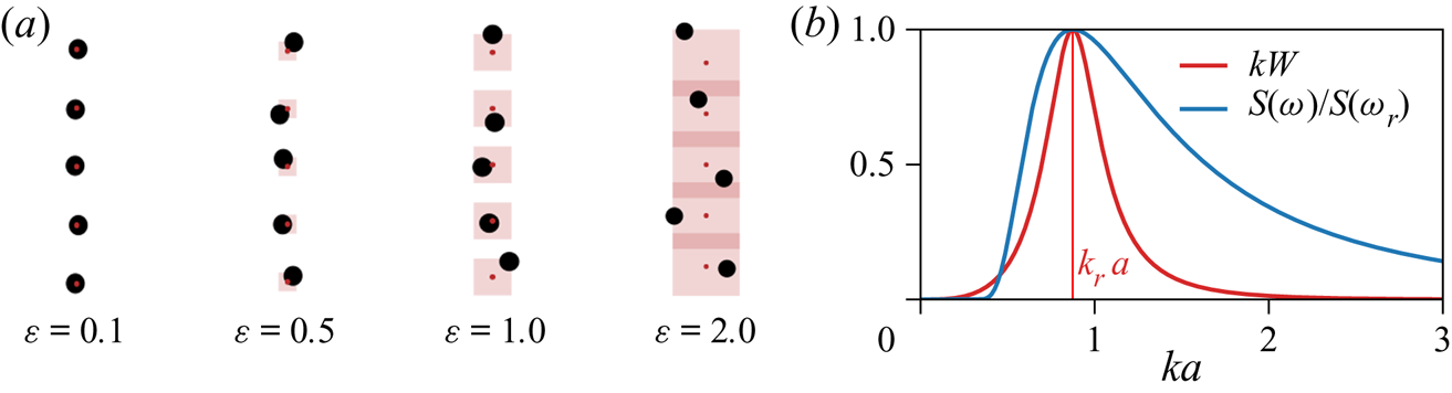
 $(d-2a)\varepsilon$, see figure 1(a). In general, we impose no further constraints on
 $\mathcal {D}(\varepsilon )$. Hereafter, we refer to the non-dimensional parameter
 $\varepsilon$ as ‘randomness’. For a given average spacing
 $d$ and randomness
 $\varepsilon$, the spatial configuration
 $\mathcal {C}(d,\varepsilon ) = \{x_1,y_1,\ldots ,x_N,y_N\}^T$ of
 $\mathcal {R}$ is a
 $2N$-dimensional random vector. Only physically feasible realizations of
 $\mathcal {C}(d,\varepsilon )$, where the bodies in
 $\mathcal {R}$ do not intersect, are considered.
(a) Realizations of  $\mathcal {R}$ arrays of mean spacing
 $d/2a = 2.9$ for increasing randomness
 $\varepsilon$, for uniformly distributed position perturbations
 $\in [-\varepsilon /2,\varepsilon /2]$. The red dots mark the body centres of the underlying
 $\mathcal {U}$ array. The shaded box represents the possible positions of bodies in
 $\mathcal {R}$. (b) Non-dimensional capture width
 $kW$ for an isolated truncated vertical cylinder WEC (
 $a/h = 0.3$,
 $H/h = 0.2$) as a function of wavenumber
 $ka$. The body-resonant wavenumber
 $k_{r} a$ is shown for reference. A Bretschneider spectrum
 $S(\omega )$ with peak wavenumber
 $k_{p}=k_{r}$ is plotted for comparison.

For simplicity, we consider WEC devices that extract power only in heave through a linear power take-off (PTO). We set the PTO damping rate  $b_{PTO}=b(\omega _{r})$, where
 $b(\omega _{r})$ is the radiation damping coefficient at the heave resonant frequency
 $\omega _{r}$ (corresponding wavenumber
 $k_{r}$) of the body. For an isolated WEC tuned to resonate with frequency
 $\omega =\omega _{r}$,
 $b_{PTO}=b(\omega _{r})$ maximizes power extraction at
 $k_{r}$ to theoretical maximum of
 $kW=1$, where
 $W$ is the capture width (Mei, Stiassnie & Yue Reference Mei, Stiassnie and Yue2005), see figure 1(b).
In monochromatic incident waves of frequency  $\omega$ and incident angle
 $\theta _{I}$, the total power
 $P$ extracted by an array of size
 $N$ and spatial configuration
 $\mathcal {C}$ is
 $P= \sum _{{j} = 1}^{N}P_j$, where
 $P_j(k,\theta _{I};\mathcal {C})=\frac 12b_{PTO}|V_j(k,\theta _{I})|^2$ is the power extracted by
 $\mathcal {B}_j$ oscillating in heave with complex velocity amplitude
 $V_j$. The power efficacy of the array is defined by the array gain
 $q(k,\theta _{I};\mathcal {C}) = P/(N P_0)$, where
 $P_0(k)$ is the power extracted by an isolated WEC device.
For unidirectional irregular seas, the total power the WEC array extracts is  $P^{S}(\theta _{I};\mathcal {C}) = \int _{\omega }S(\omega )P \,\textrm {d}\omega$, where
 $S(\omega )$ is the incident wave (frequency) spectrum. Analogous to the monochromatic case, we define the spectral array gain
 $q_{S}(\theta _{I};\mathcal {C}) = P^{S}/N P_0^{S}$, where
 $P_0^{S}$ is the power extracted by an isolated WEC in this irregular sea. The array gains
 $q$ and
 $q_{S}$ are the primary quantities of interest in this work, where
 $q$,
 $q_{S}>1$ indicates that the
 $N$-body WEC array extracts more power than
 $N$ isolated bodies due to favourable wave interactions within the array.
To obtain useful statistics, we consider random samples of  $M$ realizations of
 $\mathcal {C}(d,\varepsilon )$ to evaluate the ensemble means
 $\left \langle q \right \rangle$,
 $\left \langle q _{S}\right \rangle$ and the corresponding standard deviations
 $\sigma _q$,
 $\sigma _{q_{S}}$, where
 $\left \langle \cdot \right \rangle$ denotes ensemble mean. To evaluate the performance of a given array, we use a multiple-scattering method for fast calculation of linear wave-body interactions in arrays of bodies of arbitrary shapes and motion constraints without introducing any additional assumptions. The method is based on the approach introduced by Kagemoto & Yue (Reference Kagemoto and Yue1986) and extended by Tokić & Yue (Reference Tokić and Yue2019b) for periodic arrays. We express the incident, scattered and radiated wave fields (propagating and evanescent) in terms of partial wave expansions (Linton & McIver Reference Linton and McIver2001), and close the linear system for the unknown amplitudes of partial waves by enforcing the boundary conditions on each body. While the formulation is, in principle, exact, the resulting linear system is infinitely large, so we truncate the number of partial waves in the expansion to facilitate numerical calculation. The hydrodynamic forces, body dynamics, and the amplitudes of scattered and radiated waves for a body in the array are all functions of the partial wave amplitudes of the total incident wave potential at that body and are obtained through transfer matrices. The transfer matrices are independent of the array configuration and can be calculated for a body in isolation. The details of the method are provided in Tokić & Yue (Reference Tokić and Yue2019b).
3. Performance of randomly perturbed line arrays
We first perform systematic computations of 50-body  $\mathcal {R}$ arrays for a range of average spacing
 $d$ and randomness parameter
 $\varepsilon$ to elucidate the effect of introducing random perturbations on energy extracting performance. Hereafter, for specificity, we consider a truncated vertical cylinder WEC geometry of radius
 $a/h = 0.3$ and draft
 $H/h = 0.2$, in water depth
 $h$. Furthermore, without loss of generality, we focus on uniformly distributed position perturbations
 $X_j, Y_j \in \varepsilon (d-2a)[-1/2,1/2]$. We compute
 $M=50$ random realizations of each spatial configuration
 $\mathcal {C}(d,\varepsilon )$, which is a sufficient number to achieve convergence to within 1 % for the quantities of interest.
3.1. Performance in monochromatic waves
A defining feature of large  $\mathcal {U}$ arrays (
 $N\to \infty$) is that they exhibit Rayleigh resonances, at which the extracted power vanishes (Tokić & Yue Reference Tokić and Yue2019b). These occur at the Rayleigh wavenumbers
 $(kd)_{m}^{{cr}} = 2{\rm \pi} m/(\pm 1-\sin \theta _{I})$, regardless of the WEC body geometry.
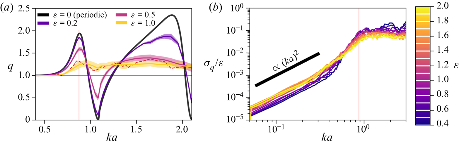
Introducing random perturbations to body positions acts to smooth out the extremes in gain  $q$ for
 $\mathcal {R}$ arrays, see figure 2(a). At
 $(kd)_{m}^{{cr}}$,
 $q$ increases with the increase in
 $\varepsilon$, and away from them
 $q$ is decreased. This is caused by the absence of coherent scattering due to the introduced random perturbations. Overall, increasing randomness
 $\varepsilon$ results in a more constant
 $\left \langle q \right \rangle$ as a function of wavenumber
 $ka$, but increases the standard deviation of gain
 $\sigma _q$. Note that
 $\left \langle q \right \rangle$ is not realized by any specific
 $\mathcal {R}$ in general.
Performance of 50-body  $\mathcal {R}$ with average spacing
 $d/2a = 2.9$ for different values of randomness
 $\varepsilon$ as a function of wavenumber
 $k$, for normal incidence. (a) Array gain
 $q$. The results show the mean
 $\left \langle q \right \rangle$ (thick solid line)
 ${\pm }1$ standard deviation
 $\sigma _q$ (band of matching colour). A single realization for
 $\varepsilon =1$ is shown in dashed red line. Performance of a periodic array with the periodicity
 $d$ is shown for comparison. (b) Standard deviation
 $\sigma _q$ of gain
 $q$. The thick black line represents
 $(ka)^2$ slope. In both plots, the red vertical line denotes the body-resonant wavenumber
 $k_{r}$.

The character of  $\sigma _q$ is markedly different depending on whether the wavenumber
 $k$ is above or below the body-resonant wavenumber
 $k_{r}$, see figure 2(b). Above
 $k_{r}$,
 $\sigma _q/\varepsilon$ is roughly constant. Below
 $k_{r}$, i.e. in the low-scattering regime
 $(ka \ll 1)$,
 $\sigma _q/\varepsilon$ scales as
 $(ka)^2$ with increasing
 $ka$.
The  $\sigma _q/\varepsilon \sim (ka)^2$ scaling can be explained using the Delta method (Oehlert Reference Oehlert1992) for the estimation of the function variance. The variance of gain can be approximated as
 $\textrm {Var} q(k,\theta _{I};\mathcal {C}) = (\boldsymbol {\nabla }_\mathcal {C} q)^T\boldsymbol {\varSigma }\boldsymbol {\nabla }_\mathcal {C} q$, where
 $\boldsymbol {\nabla }_\mathcal {C} q$ is the gradient of
 $q$ with respect to
 $\mathcal {C}$ at
 ${\mathcal {C}(d,\varepsilon =0)}$ and
 $\boldsymbol {\varSigma }$ is the covariance matrix. As the body position perturbations are independent and identically distributed random variables,
 $\boldsymbol {\varSigma }\propto \varepsilon ^2 \boldsymbol{\mathsf{I}}$, where
 $\boldsymbol{\mathsf{I}}$ is a
 $2N\times 2N$ identity matrix, leading to
 $\sigma _q/\varepsilon = \sqrt {\textrm {Var} q}/\varepsilon = \|\boldsymbol {\nabla }_\mathcal {C} q\|$. For
 $ka \ll 1$, the velocity of
 $\mathcal {B}_i$ is
 $V_{i,}\approx \omega \eta _i$, where
 $\eta _i$ is the complex free surface amplitude at
 $\mathcal {B}_i$, and
 $\boldsymbol {\nabla }_\mathcal {C} q \propto \sum _{{i} = 1}^{N} \boldsymbol {\nabla }_\mathcal {C} |\eta _i|^2$. As the scattering is weak, we can consider that only a single scattering event occurs, so the scattered wave amplitude at
 $\mathcal {B}_i$ from
 $\mathcal {B}_j$ are proportional to
 $(ka)^2(-\mathrm {i}/2{H}_0(kR_{ij})-\gamma {H}_1(k R_{ij})) = (ka)^2{h}(kR_{ij})$, where
 ${H}_n(x)\equiv {H}_n^{(1)}(x)$ is the Hankel function,
 $\gamma$ a real coefficient, and
 ${h}(x)$ a complex function. Using the complex identity
 $\boldsymbol {\nabla }_\mathcal {C} |\eta _i|^2 = 2\mathrm {Re}[\eta _i^*\boldsymbol {\nabla }_\mathcal {C}\eta _i]$ (
 $^*$ denotes complex conjugate) and the asymptotic behaviour
 $\mathrm {Re}[{h}'(x)]\sim 1/x -{\rm \pi} \gamma /2+O(x)$ for
 $x\ll 1$, the resulting scaling is
 $\sigma _q/\varepsilon \sim \mathrm {Re}[(1+(ka)^2 {h}^*)(ka)^3 {h}']\sim (ka)^2 + O((ka)^3)$.
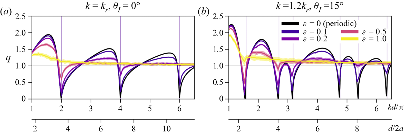
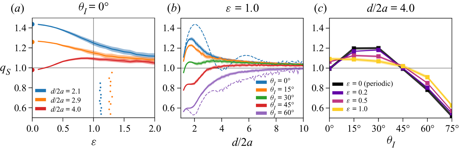
For a given wavenumber  $k$, increasing the inter-body spacing
 $d$ leads to isolated body performance (
 $q\to 1$) as, in general, the scattered and radiated wave interactions become weaker, see figure 3. This is less pronounced in
 $\mathcal {U}$ arrays as the effects from coherent scattering accumulate. Introducing random perturbations, however, results in an increased decoherence, so
 $q$ of
 $\mathcal {R}$ arrays converges to 1 with the increase in
 $d$ more rapidly than for
 $\mathcal {U}$ arrays. As a result, sufficiently perturbed
 $\mathcal {R}$ arrays will perform as isolated bodies for smaller
 $d$ than their corresponding
 $\mathcal {U}$. The rate of convergence of
 $\left \langle q \right \rangle$ to 1 increases with the increase in
 $\varepsilon$. The standard deviation
 $\sigma _q$ is not affected by variation in
 $d$.
Array gain  $q$ for 50-body
 $\mathcal {R}$ as a function of spacing
 $d$ for different randomness
 $\varepsilon$, for two wavenumbers
 $k$ and incident angles
 $\theta _{I}$. In all cases, the thickness of the banded line represents
 $\left \langle q _{S}\right \rangle \pm \sigma _{q_{S}}$. Vertical lines mark the Rayleigh wavenumbers
 $(kd)_{m}^{{cr}}$.

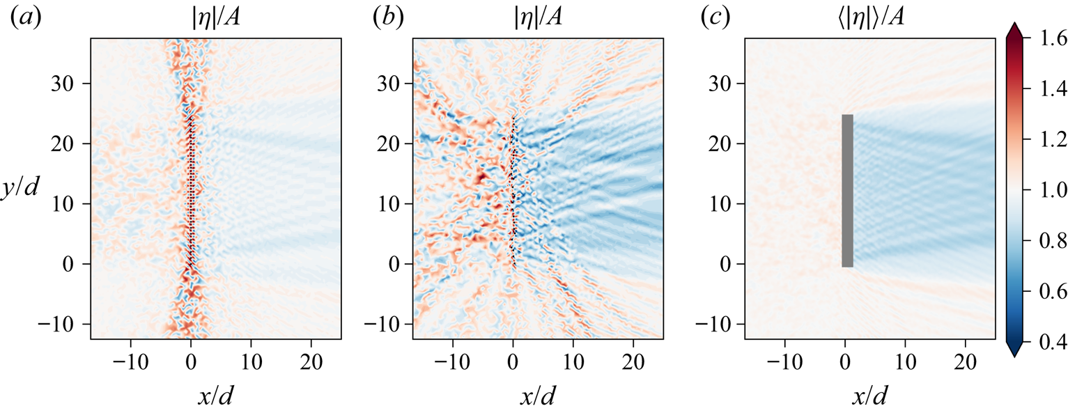
The effect of random perturbations on the free surface amplitude  $|\eta |$ around 25-body arrays of spacing
 $d/2a=3.6$ in normal incidence for
 $k=k_{r}$ is shown in figure 4. The
 $\mathcal {U}$ array for that
 $kd$ is close to a Rayleigh resonance (
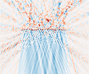
 $kd\approx 2{\rm \pi}$), associated with low power extraction. The free surface amplitude reveals that a lot of energy is scattered in the spanwise (
 $y$-) direction as a result of an emerging far-field scattering mode, rather than being extracted, see figure 4(a). By introducing random deviation to body positions, the creation of the new mode that carries energy in the spanwise direction along the array is disrupted, and
 $|\eta |$ behind
 $\mathcal {R}$ is reduced, indicating substantial extraction of energy, see figure 4(b). Rays of more pronounced
 $|\eta |$ variation are visible, but their orientation depends on the particular realization of the random configuration. The mean free surface amplitude
 $\left \langle |\eta |\right \rangle$ over all realizations reveals that, on average, almost no energy is reflected away from the array (
 $\left \langle |\eta |\right \rangle /A\approx 1$), except behind the arrays where
 $\left \langle |\eta |\right \rangle$ is significantly decreased.
Free surface amplitude  $|\eta |/A$ around 25-body WEC line arrays with
 $d/2a = 3.6$, for a monochromatic incident wave of amplitude
 $A$ and
 $k=k_{r}$ (
 $kd=2{\rm \pi}$) and
 $\theta _{I}=0^\circ$. (a)
 $\mathcal {U}$ array. (b) A sample realization of an
 $\mathcal {R}$ array with
 $\varepsilon =1$. (c) Ensemble average
 $\left \langle |\eta |\right \rangle$ of 50
 $\mathcal {R}$ arrays with
 $\varepsilon =1$. The grey region represents the extents of the area that these
 $\mathcal {R}$ arrays occupy.

Overall, these findings hold for a wide range of incident angles  $\theta _{I}$, not just
 $\theta _{I} = 0^\circ ,15^\circ$ presented here.
3.2. Performance in irregular seas
We consider the performance of  $\mathcal {R}$ arrays in irregular seas described by an incident spectrum
 $S(\omega )$, with peak wavenumber
 $k_{p}$ equal to the body-resonant wavenumber
 $k_{r}$.
Figure 5 shows the results for  $\mathcal {R}$ and
 $\mathcal {U}$ arrays in an incident wave spectrum. For specificity, a Bretschneider spectrum with
 $k_{p}=k_{r}$ is used, although the qualitative conclusions hold for general realistic wave spectra. Depending on the average spacing
 $d$, introducing
 $\varepsilon >0$ can increase or decrease the spectral gain
 $q_{S}$ of
 $\mathcal {R}$ compared with the underlying
 $\mathcal {U}$. Increasing
 $\varepsilon$ above some critical value
 $\varepsilon _{c}$, however, decreases
 $q_{S}$ for all
 $d$. For
 $\mathcal {D}(\varepsilon )$ and
 $S(\omega )$ studied here,
 $\varepsilon _{c}\approx 1$. The mean spectral gain
 $\left \langle q _{S}\right \rangle$ fluctuates less with change in
 $d$ than
 $q_{S}$ of
 $\mathcal {U}$, see figure 5(b). For the Bretschneider spectrum with
 $k_{p}=k_{r}$, the maximum achievable
 $q_{S}$ of
 $\mathcal {R}$ is lower than that of
 $\mathcal {U}$. For normal incidence and
 $\varepsilon =1$, maximum gain
 $\left \langle q _{S}\right \rangle _\text {max} = 1.3$ is achieved by
 $\mathcal {R}$ with average spacing
 $d/2a = 1.8$, while for
 $\mathcal {U}$ arrays
 ${q_{S}}_\text {max} = 1.44$ for
 $d/2a = 2.0$. There exist ranges of
 $d/2a$ and
 $\theta _{I}$, however, where
 $q_{S}$ of
 $\mathcal {R}$ is greater than that for the underlying
 $\mathcal {U}$ array. For example,
 $\mathcal {R}$ with
 $d/2a \approx 4$ outperform their underlying
 $\mathcal {U}$ for normal incidence.
Spectral array gain  $q_{S}$ of 50-body line arrays in Bretschneider-described irregular seas. (a)
 $\mathcal {R}$ arrays with three mean spacings
 $d/2a$ in normal incidence as a function of
 $\varepsilon$. Sections of two
 $\mathcal {R}$ arrays for
 $\varepsilon =1$ are shown for reference (the body colour matches the line colour for corresponding
 $d/2a$). (b)
 $\mathcal {R}$ with
 $\varepsilon =1$ as a function of
 $d/2a$. The dashed lines mark
 $q_{S}$ for
 $\mathcal {U}$ (
 $\varepsilon =0$). (c)
 $\mathcal {R}$ with different values of
 $\varepsilon$ as a function of incidence angle
 $\theta _{I}$. In all plots, the banded lines represents
 $\left \langle q _{S}\right \rangle \pm \sigma _{q_{S}}$.

For incidence angles up to  $\theta _{I}\approx 45^\circ$, the spectral gain
 $q_{S}$ of
 $\mathcal {R}$ is generally larger than 1, see figure 5(c). For large incidence angles (
 $\theta _{I}\gtrsim 45^\circ$),
 $\mathcal {R}$ perform consistently better than
 $\mathcal {U}$, and increasingly so with increase in
 $\varepsilon$. This is due to
 $q_{S}<1$ in this
 $\theta _{I}$-range for
 $\mathcal {U}$ arrays, so introducing random position perturbations leads to a more isolated-body-like performance (cf. figure 3), thus bringing
 $q_{S}$ closer to one. The standard deviation
 $\sigma _{q_{S}}$ is roughly constant for all incident angles.
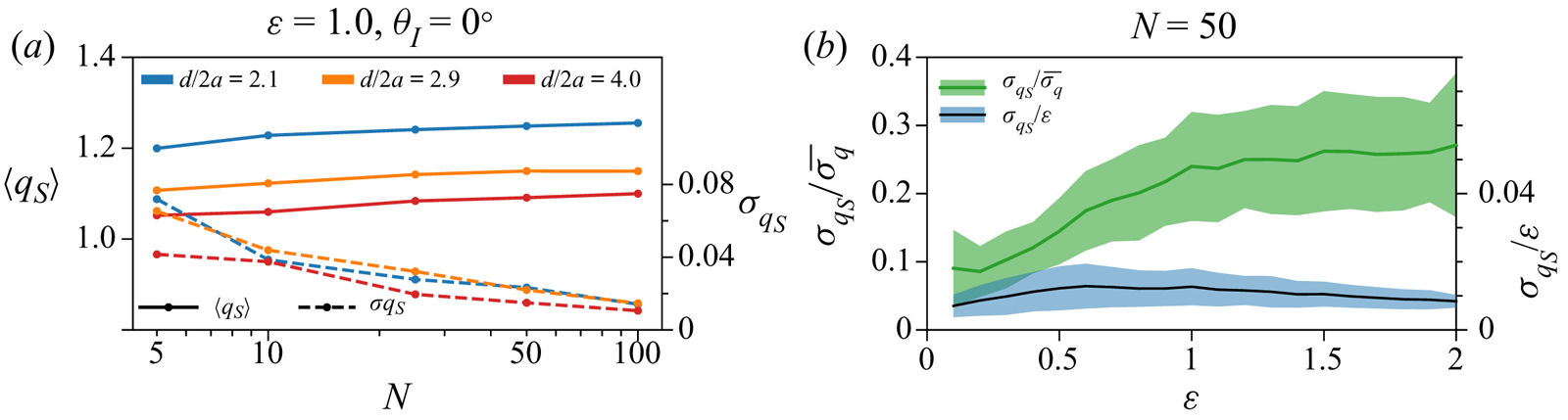
The increase of array size  $N$ increases
 $\left \langle q _{S}\right \rangle$, albeit slowly above
 $N=50$, see figure 6(a). (The same is valid for
 $\left \langle q \right \rangle$.) The standard deviation
 $\sigma _{q_{S}}$ decreases significantly with
 $N$, and for
 $N \gtrsim 50$ the deviation
 $\sigma _{q_{S}}/\left \langle q _{S}\right \rangle \lesssim 2\,\%$. It is considerably smaller than the mean ‘converged’ standard deviation
 $\overline {\sigma _q}$ (defined as mean
 $\sigma _q$ for wavenumbers larger than
 $k_{r}$), see figure 6(b). The ratio
 $\sigma _{q_{S}}/\overline {\sigma _q}$ increases with
 $\varepsilon$ for small
 $\varepsilon$ and is roughly constant (
 $\sigma _{q_{S}}/\overline {\sigma _q}\approx 0.3$) for
 $\varepsilon \gtrsim 1$. The relative deviation
 $\sigma _{q_{S}}/\varepsilon$, however, does not show an appreciable scaling with
 $\varepsilon$, so
 $\sigma _{q_{S}}/\left \langle q _{S}\right \rangle$ remains
 $O(1\,\%)$ for
 $\varepsilon$ considered here. As a result,
 $\left \langle q _{S}\right \rangle$ is a very close estimate of
 $q_{S}$ for any large (
 $N=O(100)$)
 $\mathcal {R}$ array drawn from
 $\mathcal {C}(d,\varepsilon )$.
(a) The dependence of  $\left \langle q _{S}\right \rangle$ and
 $\sigma _{q_{S}}$ on the array size
 $N$, for
 $\mathcal {R}$ arrays of three mean spacings
 $d$ and randomness
 $\varepsilon =1$. (b) The mean
 $\pm 1$ standard deviation of
 $\sigma _{q_{S}}/\overline {\sigma _q}$ (green; left axis) and of
 $\sigma _{q_{S}}/\varepsilon$ (blue; right axis) as a function of
 $\varepsilon$ for 50-body
 $\mathcal {R}$ arrays (statistics over a range of
 $d$ and
 $\theta _{I}$).

4. Comparison of optimal random and uniform WEC arrays in irregular seas
While in § 3 we elucidated how  $\mathcal {R}$ arrays perform as a function of increasing randomness and compared their performance to that of
 $\mathcal {U}$ of equal
 $d$, this does not answer what type of array is optimal for a given incident condition. In this section, we answer this question by focusing on
 $\mathcal {R}$ and
 $\mathcal {U}$ arrays of optimal spatial configuration (i.e.
 $d/2a$ optimized for maximum
 $q_{S}$) for a given incident wave spectrum and compare their performance. We limit ourselves to arrays optimized with respect to
 $d$ only since introducing additional spatial parameters results in a strongly multi-modal objective function where we cannot guarantee a global optimum. Focusing on
 $d$-optimal arrays only ensures the global optimum is easier to find, which then provides a better basis for comparison. We vary the incident spectrum parameters (bandwidth and peak frequency) to investigate whether there exist wave conditions for which
 $\mathcal {R}$ arrays are preferable over
 $\mathcal {U}$ arrays. We first perform a systematic computational analysis and then offer a heuristic argument for the results.
4.1. Comparison between optimal  $\mathcal {U}$ and $\mathcal {R}$ arrays


For a given incident wave spectrum  $S(\omega )$, the optimal uniform array
 $\mathcal {U}^*$ is the
 $\mathcal {U}$ array of spacing
 $d_{U}^*=\arg \max _d P^{S}(d,\varepsilon =0)$, extracting the maximum power
 $P_{U}^* = \max _d {P^{S}(d,\varepsilon =0)}$. Similarly, optimal randomized array
 $\mathcal {R}^*$ for a given randomness
 $\varepsilon$ is defined by the optimal mean spacing
 $d_{R}^*=\arg \max _d \left \langle P ^{S}(d,\varepsilon )\right \rangle$, and it extracts maximum power
 $P_{R}^* = \max _d \left \langle P ^{S}(d,\varepsilon )\right \rangle$. Here,
 $P_{R}^*$ is determined from the sample of
 $M=50$ realizations for every configuration
 $\mathcal {C}(d,\varepsilon )$. Using the ensemble mean to determine
 $P_{R}^*$ is a good estimate of the true maximum of
 $P^{S}(d,\varepsilon )$ over all configurations
 $\mathcal {C}(d,\varepsilon )$ because the relative standard deviation of
 $P^{S}$ (i.e.
 $\sigma _{q_{S}}/\left \langle q _{S}\right \rangle$) is small in large
 $\mathcal {R}$ arrays, see figure 6(a).
Depending on the spectrum shape, primarily its bandwidth and peak frequency relative to body-resonant frequency, the class of arrays that performs better for the incident wavefield might change. For example, while  $\mathcal {U}^*$ arrays outperform
 $\mathcal {R}^*$ in monochromatic waves as they harness the array resonances, one might consider that
 $\mathcal {R}^*$ arrays could outperform
 $\mathcal {U}^*$ arrays for some broadbanded spectra. To study the effect of the spectrum peak and width, we consider here a simple top-hat spectrum
 $S_{TH}(k;k_{p},\Delta k) = 1$ for
 $k \in [k_{p} - \Delta k/2,k_{p} + \Delta k/2]$ and 0 otherwise. This is a two-parameter
 $(k_{p},\Delta k)$ spectrum that could indicate the range of parameters for which
 $\mathcal {R}^*$ arrays outperform
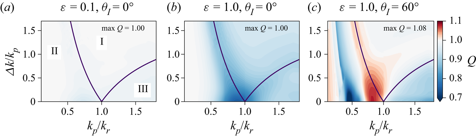
 $\mathcal {U}^*$ arrays. Three main regions can be recognized in the
 $k_{p}$–
 $\Delta k$ space, see figure 7 –
 $(k_{p}, \Delta k)$ values for which top-hat spectra contain the body-resonant wavenumber
 $k_{r}$ (region I), those for which the entire spectrum is below
 $k_{r}$ (region II), and those for which the spectrum is above
 $k_{r}$ (region III). Region I is the most interesting here because it contains the wavenumber
 $k_{r}$ for which an isolated WEC device operates optimally. Small values of
 $\Delta k/k_{p}$ (ordinate axis) represent narrow-banded spectra. To compare the maximum extracted power by the optimal
 $\mathcal {R}^*$ and
 $\mathcal {U}^*$ arrays, we define the comparison measure
 $Q(k_{p}, \Delta k)\equiv P_{R}^*/P_{U}^*$. Values of
 $Q>1$ indicate the incident wave conditions in which the random array with optimal mean spacing would outperform any uniform array.
Comparison metrics  $Q$ between the optimal
 $\mathcal {U}^*$ and
 $\mathcal {R}^*$ arrays as a function of the peak wavenumber
 $k_{p}$ and the relative bandwidth
 $\Delta k/k_{p}$ of the incident top-hat spectrum. The magenta lines separate regions I, II and III.

For a range of  $k_{p}$,
 $\Delta k$ and
 $\varepsilon$ values considered here,
 $\mathcal {U}^*$ arrays generally outperform
 $\mathcal {R}^*$ arrays for incidence angles
 $\theta _{I}\lesssim 45^\circ$, particularly for spectra in region I, indicated by
 $Q\lesssim 1$, see figure 7. In general, increasing
 $\varepsilon$ decreases
 $Q$. For long-wave top-hat spectra (region II),
 $\mathcal {R}^*$ perform as well as
 $\mathcal {U}^*$. This is the result of weak scattering for
 $ka \ll k_{r} a$, so the effect of spatial configuration on the wave interference patterns is small as well. For large incidence angles (e.g.
 $\theta _{I}=60^\circ$, figure 7c),
 $\mathcal {R}^*$ can outperform
 $\mathcal {U}^*$ for a large range of spectra in regions I and II, including the narrow-banded ones. Similar behaviour is observed for random arrays in the Bretschneider-described seas (cf. figure 5c). The optimal spacings
 $d_{U}^*$ and
 $d_{R}^*$ are of very similar values, except for
 $k_{p} \ll k_{r}$, where the scattering is low and spacing plays little role. The optimal spacing
 $d_{R}^*$ is generally such that
 $k_{p} d_{R}^* < (kd)_{1}^{{cr}}$, i.e. before where the first Rayleigh resonance would occur for the peak-wavenumber wave (cf. figure 3).
4.2. A heuristic argument for $\mathcal {U}^*$ arrays outperforming $\mathcal {R}^*$ arrays


We offer here a heuristic argument for why  $\mathcal {U}^*$ arrays outperform
 $\mathcal {R}^*$ arrays even in (broadbanded) irregular seas. Consider a line array consisting of
 $J$ large
 $\mathcal {U}$-subarrays stacked next to each other, each containing
 $\mathcal {N}_{j}$ bodies
 $({\sum }_{j}\mathcal {N}_{j} = N)$ spaced
 $d_{j}$ apart. The subarray size
 $\mathcal {N}_{j}$, the inter-body spacing
 $d_{j}$ and the subarray ordering can be arbitrary. If
 $\mathcal {N}_{j} \gg 1$, the energy extraction performance of the array can be approximated as a weighted sum of the subarray performance. In irregular seas, the extracted power
 $P^{S}(\theta _{I})$ by such an array is then approximated as
 $P^{S}(\theta _{I})\approx \tilde {P}^{S}(\theta _{I})=N\sum _{j=1}^{J}w_j P^{S}_{\infty }(\theta _{I};d_{j})$, where
 $P^{S}_{\infty }$ is the power extracted by a single body in a periodic array (or a very large
 $\mathcal {U}$ array) of spacing
 $d_{j}$, and
 $w_j = \mathcal {N}_{j} /N$ is the weight quantifying the relative size of subarray
 $j$ with respect to the whole array (
 ${\sum }_j w_j = 1$). Since
 $P^{S}_{\infty }(\theta _{I};d_{j}) \le P^{S}_{\infty }(\theta _{I};d_{U}^*)$ and
 $w_j\le 1$, the power
 $P_{U}^*\approx NP^{S}_{\infty }(\theta _{I};d_{U}^*)$ extracted by
 $\mathcal {U}^*$, which has optimal spacing
 $d_{U}^*$, is the upper bound of
 $\tilde {P}^{S}$. The
 $\mathcal {R}$ arrays we consider here are not an ordered stacking of randomly selected
 $\mathcal {U}$ subarrays, but we can reach the same conclusion. Considering a large sample of
 $\mathcal {R}$ arrays of configuration
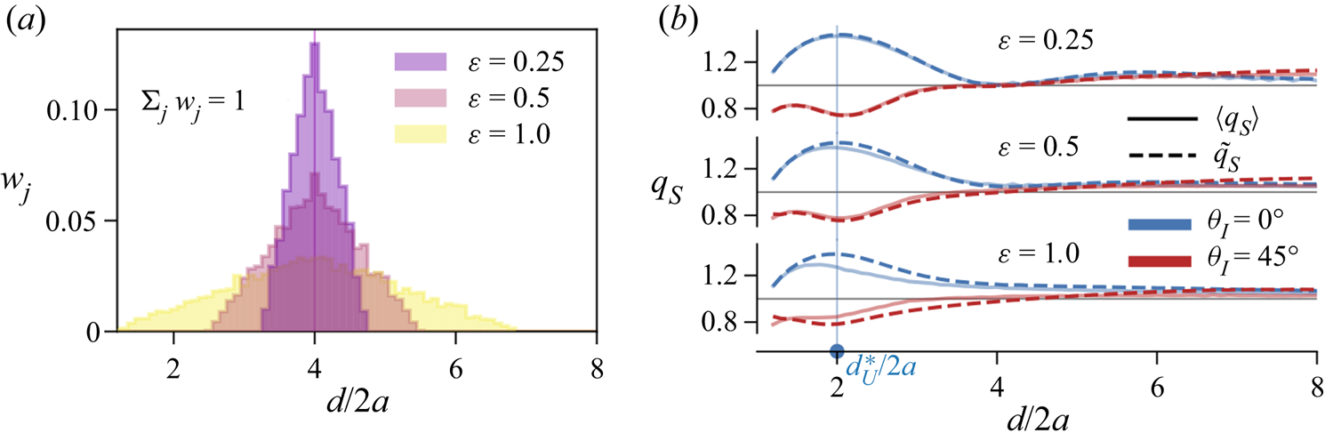
 $\mathcal {C}(d,\varepsilon )$, we can create a histogram
 $\mathcal {H}(d,\varepsilon )$ of spacings between immediate neighbours, arranged into
 $J$ bins, each centred around
 $d_{j}$,
 $j=1\ldots J$, see figure 8(a). The spread of the histogram depends on the randomness
 $\varepsilon$, but it is centred around the average spacing
 $d$. The best-case scenario for these
 $\mathcal {R}$ arrays would be if the observed inter-body distances are the result of
 $J$
 $\mathcal {U}$-subarrays of spacing
 $d_{j}$ stacked together, as discussed before. Thus,
 $P_{U}^*$ is the upper bound of
 $P^{S}$ for any configuration
 $\mathcal {C}(d,\varepsilon )$, including
 $P_{R}^*$, resulting in
 $Q \le 1$. Thus, in the absence of randomization-caused enhancements, we can consider that only
 $100\,\%\times w_{\hat {\jmath }}$ portion of
 $\mathcal {R}$ is performing optimally (
 $\hat {\jmath }$ is the index of the
 $d_{j}[\hat {\jmath }]=d_{U}^*$ bin), while the rest of the array is performing suboptimally, resulting in diminished gain.
A heuristic model for the behaviour of spectral gain  $q_{S}$. (a) Histogram
 $\mathcal {H}(d,\varepsilon )$ of observed distances in bins
 $d_{j}$ (corresponding weights
 $w_j$) in
 $\mathcal {R}$ arrays with the average spacing
 $d/2a = 4$ and varying randomness
 $\varepsilon$. (b) The comparison of ensemble mean
 $\left \langle q _{S}\right \rangle$ (solid lines) and the heuristic estimate
 $\tilde {q}_{S}$ (dashed lines) for Bretschneider spectrum for increasing level of
 $\varepsilon$; colours correspond to the incident angle
 $\theta _{I}$. The vertical line represents the optimal spacing
 $d_{U}^*$ (maximum extraction
 $\mathcal {U}^*$ array).

The heuristic estimate  $\tilde {q}_{S}(\theta _{I},d) = \tilde {P}^{S}/N P_0^{S}$ closely matches the observed mean spectral gain
 $\left \langle q _{S}\right \rangle$ of
 $\mathcal {R}$ arrays for a wide range of randomness
 $\varepsilon$ and incident angles
 $\theta _{I}$, see figure 8(b). For small values of
 $\varepsilon$,
 $\tilde {q}_{S}$ closely matches
 $\left \langle q _{S}\right \rangle$, as expected. Despite being a crude estimate,
 $\tilde {q}_{S}$ approximates
 $\left \langle q _{S}\right \rangle$ well even for large values of
 $\varepsilon$. In normal incidence,
 $\left \langle q _{S}\right \rangle <\tilde {q}_{S}$ for all
 $d$; hence
 $Q < 1$, as previously argued. For large incidence angles (e.g.
 $\theta _{I}=45^\circ$ in figure 8b),
 $\tilde {q}_{S}$ still approximates
 $\left \langle q _{S}\right \rangle$ well, but it is no longer an upper bound to it. This results from the consistent underperformance of
 $\mathcal {U}$ arrays as compared with
 $\mathcal {R}$ arrays for large
 $\theta _{I}$.
5. Discussion
From a computational aspect, the results presented here form the largest systematic analysis of randomly perturbed WEC arrays to date, consisting of  ${\sim }5\times 10^4$ simulations that take into account full wave-body interactions and multiple scattering in large arrays. We conducted the computations predominantly on arrays consisting of
 $N=50$ bodies, and we show that further increase in array size does not alter the quantitative results by more than
 $O(1\,\%)$. While the quantitative values reported here would vary for different body geometry or perturbation distribution
 $\mathcal {D}(\varepsilon )$, the overall conclusions presented here are still expected to hold.
For a given uniform array  $\mathcal {U}$ with spacing
 $d$, introducing position perturbations to obtain randomized arrays
 $\mathcal {R}$ acts to smooth out the uneven performance of
 $\mathcal {U}$ in monochromatic waves, resulting in an improved performance of
 $\mathcal {R}$ over
 $\mathcal {U}$ in some cases. For some ranges of average spacing
 $d/2a$, randomization also leads to higher spectral gains
 $\left \langle q _{S}\right \rangle$ in irregular seas. For certain
 $\mathcal {R}$ configurations,
 $\left \langle q _{S}\right \rangle (\varepsilon )$ has a maximum at
 $\varepsilon =\varepsilon _{c}>0$. For the uniformly distributed position perturbations we consider here, this value is
 $\varepsilon _{c}\approx 1$ (figure 5). Generally, increasing
 $\varepsilon$ above
 $\varepsilon _{c}$ diminishes the performance for any
 $\mathcal {R}$ as it tends to resemble the performance of a collection of isolated WECs (
 $q_{S}\to 1$).
The large gains from wave interactions in  $\mathcal {R}$ arrays occur for relatively closely spaced configurations, see figures 3 and 5(b). In
 $\mathcal {U}$ arrays, although gain converges to 1 in the supremum limit, relatively large gains can even occur for large spacing
 $d/2a$ as a result of fluctuations in energy extraction caused by coherent scattering and the associated resonant effects. In
 $\mathcal {R}$ arrays this does not occur, and the gain monotonically approaches the isolated body limit of 1 for large
 $d/2a$ in both monochromatic and irregular waves. For
 $\varepsilon \approx 1$, appreciable changes occur for mean
 $d/2a \lesssim 4$. For
 $\varepsilon =1$, for example, relatively large gain of
 $\left \langle q \right \rangle \approx 1.4$ is achieved by
 $\mathcal {R}$ with
 $d/2a = 2.2$ in monochromatic waves of body-resonant wavenumber
 $k=k_{r}$; and
 $\left \langle q _{S}\right \rangle \approx 1.3$ for
 $\mathcal {R}$ with
 $d/2a = 1.8$ in unidirectional irregular seas described by a Bretschneider spectrum.
For a given incidence spectrum, we compare uniform arrays  $\mathcal {U}^*$ optimized with respect to
 $d$, with random arrays
 $\mathcal {R}^*$ optimized with respect to mean
 $d$ and given values of
 $\varepsilon$. By considering a wide range of incident wave spectra in terms of their bandwidth and peak frequency, we find that, in general,
 $\mathcal {U}^*$ outperforms
 $\mathcal {R}^*$ for incidence angles
 $\theta _{I}\lesssim 45^\circ$. In monochromatic waves and narrow-banded spectra, this is expected due to the favourable coherent scattering and associated resonant phenomena. For broadbanded incident spectra, one might expect
 $\mathcal {R}$ to outperform
 $\mathcal {U}$ due to elimination, as a result of randomization, of regions in wavenumber space associated with low extraction and destructive interference. This turns out not to be the case, and we provide a heuristic argument for the upper bound of spectral gain (valid for
 $\mathcal {R}$ for
 $\theta _{I}\lesssim 45^\circ$) to support this finding (§ 4.2). The same heuristic argument should also hold for the gain of chirped WEC arrays, where the increased free surface amplitude due to the trapping of incident waves occurs only in a relatively small portion of the array, while it is diminished in the rest of the array (Archer et al. Reference Archer, Wolgamot, Orszaghova, Bennetts, Peter and Craster2020).
It should be noted that  $\mathcal {U}^*$ arrays do not represent optimal line arrays of general inter-body spacing, let alone those of a general spatial configuration. Optimizing for general spatial configuration can further increase energy extraction (Tokić & Yue Reference Tokić and Yue2019a), so
 $\mathcal {U}^*$ represent the lower bound of energy extraction of optimal arrays.
This work considers linear wave-body and wave-wave interactions only, i.e. assuming that the wave steepness and body motion amplitude relative to wave amplitude are small. In certain periodic arrays (and weakly perturbed randomized arrays), the local wave and body oscillation amplitudes can be very large for incident wave frequencies related to array resonances, especially for those related to trapped waves (Tokić & Yue Reference Tokić and Yue2019b). In such cases, the linear assumption is no longer valid, and a nonlinear interaction theory should be employed. Studies on weakly nonlinear interactions in arrays of surge-type devices (Michele, Renzi & Sammarco Reference Michele, Renzi and Sammarco2019; Michele & Renzi Reference Michele and Renzi2019) show that nonlinear resonance effects can be substantial. With the increase of randomness, however, the resonance effects and the associated large amplitudes are significantly diminished, so the linear theory should be even more generally valid.
Funding
This research is financially supported by the Office of Naval Research.
Declaration of interests
The authors report no conflict of interest.