2 Problem definition

In the high-order simulation of nonlinear waves using the Euler equations in Zakharov form, a key step is to obtain an expansion for the surface vertical velocity $\unicode[STIX]{x1D719}_{z}$ given the surface elevation $\unicode[STIX]{x1D702}(x,t)$ and the surface potential $\unicode[STIX]{x1D719}^{s}(x,t)\equiv \unicode[STIX]{x1D719}(x,z=\unicode[STIX]{x1D702}(x),t)$ . We briefly review the procedure for this expansion, starting from the Euler equations. While the formulation is first established for a one-dimensional surface, we generalize our main results to two-dimensional surfaces in § 5. Hereafter, gravitational acceleration and fluid density are unity upon proper choice of time and mass units:

(2.1) $$\begin{eqnarray}\displaystyle & \unicode[STIX]{x1D702}_{t}+\unicode[STIX]{x1D719}_{x}^{s}\unicode[STIX]{x1D702}_{x}-(1+\unicode[STIX]{x1D702}_{x}^{2})\unicode[STIX]{x1D719}_{z}=0, & \displaystyle\end{eqnarray}$$

(2.2) $$\begin{eqnarray}\displaystyle & \unicode[STIX]{x1D719}_{t}^{s}+\unicode[STIX]{x1D702}+{\textstyle \frac{1}{2}}\unicode[STIX]{x1D719}_{x}^{s}\unicode[STIX]{x1D719}_{x}^{s}-{\textstyle \frac{1}{2}}(1+\unicode[STIX]{x1D702}_{x}^{2})\unicode[STIX]{x1D719}_{z}^{2}=0. & \displaystyle\end{eqnarray}$$

To close (2.1) and (2.2), we need to express the surface vertical velocity $\unicode[STIX]{x1D719}_{z}\equiv \unicode[STIX]{x2202}\unicode[STIX]{x1D719}/\unicode[STIX]{x2202}z|_{z=\unicode[STIX]{x1D702}}$ in terms of $\unicode[STIX]{x1D719}^{s}$ and $\unicode[STIX]{x1D702}$ . This requires the solution of $\unicode[STIX]{x1D719}(x,z)$ from a boundary value problem (for simplicity, we neglect the $t$ dependence and also assume deep water):

(2.3) $$\begin{eqnarray}\frac{\unicode[STIX]{x2202}^{2}\unicode[STIX]{x1D719}}{\unicode[STIX]{x2202}x^{2}}+\frac{\unicode[STIX]{x2202}^{2}\unicode[STIX]{x1D719}}{\unicode[STIX]{x2202}z^{2}}=0,\quad \text{for}~z\leqslant \unicode[STIX]{x1D702}(x),\end{eqnarray}$$

subject to

(2.4) $$\begin{eqnarray}\displaystyle & \unicode[STIX]{x1D719}=\unicode[STIX]{x1D719}^{s},\quad \text{on}~z=\unicode[STIX]{x1D702}(x), & \displaystyle\end{eqnarray}$$

(2.5) $$\begin{eqnarray}\displaystyle & \unicode[STIX]{x1D735}\unicode[STIX]{x1D719}\rightarrow 0,\quad \text{on}~z\rightarrow -\infty , & \displaystyle\end{eqnarray}$$

and, say, horizontally periodic boundary condition. Since only $\unicode[STIX]{x1D719}_{z}$ is needed, the solution of the boundary value problem (BVP) can be cast into a Dirichlet–Neumann operation (DNO) $\hat{D}$ , which solves the vertical derivatives $\hat{D}\unicode[STIX]{x1D719}^{s}=\unicode[STIX]{x1D719}_{z}$ from boundary values $\unicode[STIX]{x1D719}^{s}$ .

We assume that $\unicode[STIX]{x1D702}(x)$ and $\unicode[STIX]{x1D719}^{s}(x)$ are small quantities, and consider a perturbation expansion of $\unicode[STIX]{x1D6F7}(x)\equiv \unicode[STIX]{x1D719}(x,z=0)=\sum _{m=1}^{\infty }\unicode[STIX]{x1D6F7}^{(m)}(x)$ . Expressing the surface potential $\unicode[STIX]{x1D719}^{s}$ as a Taylor-series expansion around $z=0$ and solving the inversion problem at each order, we obtain

(2.6a,b ) $$\begin{eqnarray}\unicode[STIX]{x1D6F7}^{(1)}=\unicode[STIX]{x1D719}^{s},\quad \text{and}\quad \unicode[STIX]{x1D6F7}^{(m)}=-\mathop{\sum }_{n=1}^{m-1}\frac{\unicode[STIX]{x1D702}^{n}}{n!}\unicode[STIX]{x1D705}^{n}\unicode[STIX]{x1D6F7}^{(m-n)},\quad m>1.\end{eqnarray}$$

In (2.6) we have introduced an operator $\unicode[STIX]{x1D705}$ , where $\unicode[STIX]{x1D705}\unicode[STIX]{x1D6F7}$ multiplies each Fourier coefficient of $\unicode[STIX]{x1D6F7}$ by its corresponding wavenumber magnitude $|k|$ . This definition of $\unicode[STIX]{x1D705}$ is due to the BVP (2.3)–(2.5), which renders the potential field representable by eigenfunctions $\exp (\text{i}kx+|k|z)$ . As a result, $\unicode[STIX]{x2202}\unicode[STIX]{x1D719}/\unicode[STIX]{x2202}z|_{z=0}$ is equivalent to $\unicode[STIX]{x1D705}\unicode[STIX]{x1D6F7}$ .

We construct $\unicode[STIX]{x1D719}_{z}^{(m)}$ at each order, by a Taylor-series expansion

(2.7) $$\begin{eqnarray}\unicode[STIX]{x1D719}_{z}^{(m)}=\mathop{\sum }_{n=0}^{m-1}\frac{\unicode[STIX]{x1D702}^{n}}{n!}\unicode[STIX]{x1D705}^{n+1}\unicode[STIX]{x1D6F7}^{(m-n)}.\end{eqnarray}$$

With $\unicode[STIX]{x1D6F7}$ expressed by (2.6), the final expression of $\unicode[STIX]{x1D719}_{z}^{(m)}$ can be obtained in terms of $\unicode[STIX]{x1D719}^{s}$ and $\unicode[STIX]{x1D702}$ . Using an operator expansion of the DNO, $\hat{D}\unicode[STIX]{x1D719}^{s}=\sum _{m=1}^{\infty }\hat{D}_{m}\unicode[STIX]{x1D719}^{s}$ , where $\hat{D}_{m}\unicode[STIX]{x1D719}^{s}\equiv \unicode[STIX]{x1D719}_{z}^{(m)}$ , the solution is obtained for the first three orders:

(2.8a ) $$\begin{eqnarray}\left.\begin{array}{@{}c@{}}\unicode[STIX]{x1D719}_{z}^{(1)}\equiv \hat{D}_{1}\unicode[STIX]{x1D719}^{s}=\unicode[STIX]{x1D705}\unicode[STIX]{x1D719}^{s},\\ \unicode[STIX]{x1D719}_{z}^{(2)}\equiv \hat{D}_{2}\unicode[STIX]{x1D719}^{s}=[-\unicode[STIX]{x1D705}\unicode[STIX]{x1D702}\unicode[STIX]{x1D705}+\unicode[STIX]{x1D702}\unicode[STIX]{x1D705}^{2}]\unicode[STIX]{x1D719}^{s},\\ \unicode[STIX]{x1D719}_{z}^{(3)}\equiv \hat{D}_{3}\unicode[STIX]{x1D719}^{s}=\left[\unicode[STIX]{x1D705}\unicode[STIX]{x1D702}\unicode[STIX]{x1D705}\unicode[STIX]{x1D702}\unicode[STIX]{x1D705}-\unicode[STIX]{x1D702}\unicode[STIX]{x1D705}^{2}\unicode[STIX]{x1D702}\unicode[STIX]{x1D705}+{\textstyle \frac{1}{2}}(\unicode[STIX]{x1D702}^{2}\unicode[STIX]{x1D705}^{3}-\unicode[STIX]{x1D705}\unicode[STIX]{x1D702}^{2}\unicode[STIX]{x1D705}^{2})\right]\unicode[STIX]{x1D719}^{s},\end{array}\right\}\end{eqnarray}$$

and in a general form (Milder Reference Milder1990):

(2.8b ) $$\begin{eqnarray}\hat{D}_{m}=\frac{1}{m-1}\mathop{\sum }_{j=1}^{m-1}[\unicode[STIX]{x1D702},\hat{D}_{j}]\hat{D}_{m-j},\quad m>1,\end{eqnarray}$$

where $[\unicode[STIX]{x1D702},\hat{D}_{j}]\equiv \unicode[STIX]{x1D702}\hat{D}_{j}-\hat{D}_{j}\unicode[STIX]{x1D702}$ is a commutator.

To illustrate the computational difficulty associated with (2.8) in describing long–short wave interaction, we consider two modes with wavenumber and amplitude of respectively $k_{S}$ , $a_{S}$ and $k_{L}$ , $a_{L}$ , for which $\unicode[STIX]{x1D6FE}\equiv k_{S}/k_{L}\gg 1$ and $k_{S}a_{S}\sim k_{L}a_{L}\sim O(\unicode[STIX]{x1D716})$ . In this situation, $k_{S}a_{L}\sim \unicode[STIX]{x1D6FE}\unicode[STIX]{x1D716}$ is a large number which increases with $\unicode[STIX]{x1D6FE}$ . The presence of large terms involving $k_{S}a_{L}$ in $\unicode[STIX]{x1D719}_{z}^{(m)}$ (for $m>1$ ) can be illustrated, as an example, by substituting these two modes in the first term of $\unicode[STIX]{x1D719}_{z}^{(2)}$ in (2.8a ): $\unicode[STIX]{x1D705}\unicode[STIX]{x1D702}\unicode[STIX]{x1D705}\unicode[STIX]{x1D719}^{s}\sim \unicode[STIX]{x1D705}(\unicode[STIX]{x1D702}_{L}+\unicode[STIX]{x1D702}_{S})\unicode[STIX]{x1D705}(\unicode[STIX]{x1D719}_{L}^{s}+\unicode[STIX]{x1D719}_{S}^{s})$ , and the cross-term involves a large quantity $O(k_{S}a_{L})$ associated with the term $\unicode[STIX]{x1D705}\unicode[STIX]{x1D702}_{L}\unicode[STIX]{x1D705}\unicode[STIX]{x1D719}_{S}^{s}\sim O(k_{S}^{2}a_{S}a_{L})\sim O(\unicode[STIX]{x1D6FE}\unicode[STIX]{x1D716}^{2})$ . Applying this substitution to higher orders of $\unicode[STIX]{x1D719}_{z}$ , we can generally conclude that terms of $O((k_{S}a_{L})^{m-1}\unicode[STIX]{x1D716})=O(\unicode[STIX]{x1D6FE}^{m-1}\unicode[STIX]{x1D716}^{m})$ are always present in $\unicode[STIX]{x1D719}_{z}^{(m)}$ . For $m\gg 1$ (and $\unicode[STIX]{x1D6FE}\gg 1$ ), these terms become divergent. This has called into question the validity and efficacy of the expansion (2.8) for long–short wave interactions to high order. In the following, we evaluate the effect of these terms and the convergence property of (2.8) using both numerical and theoretical analyses.

3 Numerical illustration

We consider the numerical implementation of (2.8), facilitated by fast Fourier transform (FFT) as in HOS. In particular, we construct a BVP (2.3)–(2.5), with prescribed $\unicode[STIX]{x1D702}(x)$ and $\unicode[STIX]{x1D719}^{s}(x)$ containing long and short wave components,

(3.1) $$\begin{eqnarray}\displaystyle & \unicode[STIX]{x1D702}(x)=a_{S}\cos (k_{S}x)+a_{L}\cos (k_{L}x), & \displaystyle\end{eqnarray}$$

(3.2) $$\begin{eqnarray}\displaystyle & \unicode[STIX]{x1D719}^{s}(x)=a_{S}\sin (k_{S}x)\exp (k_{S}\unicode[STIX]{x1D702}(x))+a_{L}\sin (k_{L}x)\exp (k_{L}\unicode[STIX]{x1D702}(x)), & \displaystyle\end{eqnarray}$$

for which an analytical solution of $\unicode[STIX]{x1D719}_{z}$ exists:

(3.3) $$\begin{eqnarray}\unicode[STIX]{x1D719}_{z}^{e}(x)=a_{S}k_{S}\sin (k_{S}x)\exp (k_{S}\unicode[STIX]{x1D702}(x))+a_{L}k_{L}\sin (k_{L}x)\exp (k_{L}\unicode[STIX]{x1D702}(x)).\end{eqnarray}$$

This BVP, with closed-form solution, provides a model problem whereby the convergence property of (2.8) can be examined in the presence of long and short wave modes, although (3.2) and (3.3) do not exactly correspond to physical long–short wave interactions. Specifically for the examination, we fix $k_{L}=1$ , $a_{L}k_{L}=a_{S}k_{S}=0.2$ and consider two values of $k_{S}=10$ and $100$ , i.e. wavelength ratios $\unicode[STIX]{x1D6FE}=10$ and $100$ . We calculate $\unicode[STIX]{x1D719}_{z}$ by the series (2.8) on a grid of $N_{x}=4096$ (over the wavelength of the long wave).

For a truncated numerical solution up to order $m=M$ , we define a relative error for $\unicode[STIX]{x1D719}_{z}^{[M]}\equiv \sum _{m=1}^{M}\unicode[STIX]{x1D719}_{z}^{(m)}$ as

(3.4) $$\begin{eqnarray}\text{err}(M)=\Vert \unicode[STIX]{x1D719}_{z}^{e}(x)-\unicode[STIX]{x1D719}_{z}^{[M]}(x)\Vert _{2}/\Vert \unicode[STIX]{x1D719}_{z}^{e}(x)\Vert _{2},\end{eqnarray}$$

and plot in figure 1 the error $\text{err}(M)$ with increasing $M$ using different (relative) machine precisions $\unicode[STIX]{x1D707}$ . We see that for given $\unicode[STIX]{x1D6FE}$ and $\unicode[STIX]{x1D707}$ , the HOS exponential convergence of $\unicode[STIX]{x1D719}_{z}^{[M]}$ with $M$ is lost after some value of $M=M_{d}$ , above which the solution diverges. Specifically, for $\unicode[STIX]{x1D6FE}=10$ , $M_{d}=4$ , 11 and ${>}20$ ; and for $\unicode[STIX]{x1D6FE}=100$ , $M_{d}=4$ , 9 and 18, for single, double and quadruple precision, corresponding to $\unicode[STIX]{x1D707}=O(10^{-7})$ , $O(10^{-16})$ and $O(10^{-34})$ respectively.

Figure 1.

Relative error $\text{err}(M)$ with increase of nonlinearity order $M$ , using respectively single (

), double (

) and quadruple (

) precision, for (a) $\unicode[STIX]{x1D6FE}=10$ and (b) $\unicode[STIX]{x1D6FE}=100$ .

For $M<M_{d}$ , the exponential convergence provides numerical evidence of cancellation of divergent terms of $O(k_{S}a_{L})$ at each order $m$ . However, as $M$ increases, the numerics become ill-conditioned in the calculation of the small term $\unicode[STIX]{x1D719}_{z}^{(m)}=O(\unicode[STIX]{x1D716}^{m})$ from the difference of large terms $G^{(m)}\sim (k_{S}a_{L})^{m-1}\unicode[STIX]{x1D716}\sim \unicode[STIX]{x1D6FE}^{m-1}\unicode[STIX]{x1D716}^{m}$ . Comparing figures 1(a) and 1(b), it is clear that the numerical ill-conditioning is more severe for greater values of $\unicode[STIX]{x1D6FE}$ (hence $G^{(m)}$ ).

To characterize the numerical ill-conditioning in the calculation of (2.8), we define a condition number

(3.5) $$\begin{eqnarray}\unicode[STIX]{x1D70E}(m)=\Vert G^{(m)}(k)\Vert _{\infty }/\Vert \unicode[STIX]{x1D719}_{z}^{(m)}(k)\Vert _{\infty },\end{eqnarray}$$

where $G^{(m)}(k)$ is the largest term involved in the calculation of (2.8), and $\unicode[STIX]{x1D719}_{z}^{(m)}(k)$ is the (correct) modal amplitude of the vertical velocity, both as functions of order $m$ and mode $k$ . In (3.5), we use the infinite norm to emphasize the maximum values of the modal amplitudes $G^{(m)}(k)$ and $\unicode[STIX]{x1D719}_{z}^{(m)}(k)$ , with the former representing the level of the largest number involved in the calculation, and the latter the level of the dominant magnitude of the solution. As $\unicode[STIX]{x1D70E}(m)$ increases, the error due to the large terms increases, which results in numerical ill-conditioning beyond some threshold value of $m$ . This can be combined with the machine precision $\unicode[STIX]{x1D707}$ to establish a criterion to predict the order $m$ at which the numerical divergence occurs (as the machine error due to the large term is of the order of the desired result),

(3.6) $$\begin{eqnarray}\unicode[STIX]{x1D707}\unicode[STIX]{x1D70E}(m)\gtrsim O(1).\end{eqnarray}$$

Figure 2 plots $\unicode[STIX]{x1D707}\unicode[STIX]{x1D70E}(m=M)$ and $\text{err}(M)$ with increasing $M$ , for the two $\unicode[STIX]{x1D6FE}$ values using single and double precision. It can be seen that the magnitude of $\text{err}(M)$ increases rapidly for $\unicode[STIX]{x1D707}\unicode[STIX]{x1D70E}(M)\gtrsim O(1)$ , so that (3.5) and (3.6) are effective means to characterize the numerical ill-conditioning.

Figure 2.

$\unicode[STIX]{x1D707}\unicode[STIX]{x1D70E}(M)$ (

) and $\text{err}(M)$ (

) with the increase of $M$ , for $\unicode[STIX]{x1D6FE}=10$ with (a) single and (b) double precision, and $\unicode[STIX]{x1D6FE}=100$ with (c) single and (d) double precision. The position of $\unicode[STIX]{x1D707}\unicode[STIX]{x1D70E}=1$ is indicated by – – –. Note that in these results $\unicode[STIX]{x1D719}_{z}^{(m=M)}(k)$ in (3.5) is evaluated using quadruple precision.

4 Analytical cancellation and convergence

In this section, we consider the cancellation of the divergent terms involving $k_{S}a_{L}$ theoretically to high order. Specifically, we demonstrate the analytical cancellation of these terms at arbitrary order of $\unicode[STIX]{x1D719}_{z}^{(m)}$ , and that the perturbation expansion of $\unicode[STIX]{x1D719}_{z}$ is bounded by the power series of the small parameter of modal wave steepness.

4.1 Interaction of a single long wave and a single short wave

We first show the cancellation of terms proportional to $k_{S}a_{L}$ in $\unicode[STIX]{x1D719}_{z}^{(2)}$ for a wave field with two modes $k_{S}\gg k_{L}$ . (Note that $\unicode[STIX]{x1D719}_{z}^{(1)}$ , by definition, is free of terms involving $k_{S}a_{L}$ .)

Following a similar procedure as in Brueckner & West (Reference Brueckner and West1988), we write $\unicode[STIX]{x1D702}$ and $\unicode[STIX]{x1D719}^{s}$ as summations of the long and short wave modes:

(4.1a,b ) $$\begin{eqnarray}\unicode[STIX]{x1D702}=\mathop{\sum }_{r=k_{L},k_{S}}a_{r}\text{e}^{\text{i}rx}+\text{c.c.},\quad \text{and}\quad \unicode[STIX]{x1D719}^{s}=\mathop{\sum }_{p=k_{L},k_{S}}(a_{p}\unicode[STIX]{x1D714}_{p}/k_{p})\text{e}^{\text{i}px}+\text{c.c.},\end{eqnarray}$$

where $\unicode[STIX]{x1D714}_{p}$ is the angular frequency at mode $p$ and c.c. denotes the complex conjugate. We consider both the long and short wave steepnesses $k_{S}a_{S}$ , $k_{L}a_{L}$ to be small, say bounded by some parameter $\unicode[STIX]{x1D716}\ll 1$ , but do not necessarily constrain them to be of similar magnitude.

At second order, we consider the Fourier components of $\unicode[STIX]{x1D719}_{z}^{(2)}=[\unicode[STIX]{x1D702},\unicode[STIX]{x1D705}]\unicode[STIX]{x1D705}\unicode[STIX]{x1D719}^{s}$ and, in particular, a component that results from interaction between a mode $r$ in $\unicode[STIX]{x1D702}$ and mode $p$ in $\unicode[STIX]{x1D719}^{s}$ . For brevity, we use the symbol ‘ $=\sim$ ’ to denote the form of such a component:

(4.2) $$\begin{eqnarray}\unicode[STIX]{x1D719}_{z}^{(2)}=[\unicode[STIX]{x1D702},\unicode[STIX]{x1D705}]\unicode[STIX]{x1D705}\unicode[STIX]{x1D719}^{s}=\sim \frac{\unicode[STIX]{x1D714}_{p}}{k_{p}}a_{p}a_{r}(|p|^{2}-|p||p+r|)\text{e}^{\text{i}(p+r)x}.\end{eqnarray}$$

The full expression for $\unicode[STIX]{x1D719}_{z}^{(2)}$ can be obtained by summing all the interactions between the modes of $\unicode[STIX]{x1D702}$ and $\unicode[STIX]{x1D719}^{s}$ using (4.1) and (4.2). At second order, this results in the summation of $4\times 4=16$ terms as $\unicode[STIX]{x1D702}$ and $\unicode[STIX]{x1D719}^{s}$ can each take the long and short modes and their complex conjugates. After cancellations of the divergent terms (e.g. when $p=k_{S}$ and $r=k_{L}$ , terms of $(k_{S}a_{S})(k_{S}a_{L})\sim O(\unicode[STIX]{x1D6FE}\unicode[STIX]{x1D716}^{2})$ cancel in (4.2)), we reach the expression

(4.3) $$\begin{eqnarray}\displaystyle \unicode[STIX]{x1D719}_{z}^{(2)} & = & \displaystyle \frac{\unicode[STIX]{x1D714}_{L}}{k_{L}}(k_{L}a_{L})(k_{L}a_{L}^{\ast })+\frac{\unicode[STIX]{x1D714}_{S}}{k_{S}}(k_{S}a_{S})(k_{S}a_{S}^{\ast })-\frac{\unicode[STIX]{x1D714}_{L}}{k_{L}}(k_{L}a_{L})^{2}\text{e}^{2\text{i}k_{L}x}-\frac{\unicode[STIX]{x1D714}_{S}}{k_{S}}(k_{S}a_{S})^{2}\text{e}^{2\text{i}k_{S}x}\nonumber\\ \displaystyle & & \displaystyle -\,\left(\frac{\unicode[STIX]{x1D714}_{L}}{k_{L}}+\frac{\unicode[STIX]{x1D714}_{S}}{k_{S}}\right)(k_{L}a_{L})(k_{S}a_{S})\text{e}^{\text{i}(k_{S}+k_{L})x}+\left(\frac{\unicode[STIX]{x1D714}_{S}}{k_{S}}-\frac{\unicode[STIX]{x1D714}_{L}}{k_{L}}\right)(k_{L}a_{L}^{\ast })(k_{S}a_{S})\text{e}^{\text{i}(k_{S}-k_{L})x}\nonumber\\ \displaystyle & & \displaystyle +\,2\frac{\unicode[STIX]{x1D714}_{L}}{k_{L}}(k_{L}a_{L}^{\ast })(k_{L}a_{S})\text{e}^{\text{i}(k_{S}-k_{L})x}+\text{c.c.},\end{eqnarray}$$

where $a_{L,S}^{\ast }$ is the complex conjugate of $a_{L,S}$ . In (4.3), the first four terms represent the second-order self-interaction of the long/short wave itself. The remaining terms represent the long–short wave interactions involving sums and differences of the respective wavenumbers. All of the terms are free of the factor $k_{S}a_{L}$ . The first six terms are of $O(\unicode[STIX]{x1D716}^{2})$ , involving only the modal wave steepness, and the seventh term is of $O(\unicode[STIX]{x1D716}^{2}/\unicode[STIX]{x1D6FE})\ll O(\unicode[STIX]{x1D716}^{2})$ . Therefore, $\unicode[STIX]{x1D719}_{z}^{(2)}$ is rigorously bounded by $O(\unicode[STIX]{x1D716}^{2})$ .

This analysis can be extended to show the cancellation of divergent terms at the third order $\unicode[STIX]{x1D719}_{z}^{(3)}$ . For this purpose, we use (2.8b ) to obtain $\unicode[STIX]{x1D719}_{z}^{(3)}=([\unicode[STIX]{x1D702},\unicode[STIX]{x1D705}]\unicode[STIX]{x1D719}_{z}^{(2)}+[\unicode[STIX]{x1D702},\hat{D}_{2}]\unicode[STIX]{x1D719}_{z}^{(1)})/2$ . Since the operator $[\unicode[STIX]{x1D702},\unicode[STIX]{x1D705}]$ has been shown (in the proof for $\unicode[STIX]{x1D719}_{z}^{(2)}$ ) to not produce any divergent terms when acting on well-bounded variables such as $\unicode[STIX]{x1D719}_{z}^{(2)}$ , only the second term in the expression of $\unicode[STIX]{x1D719}_{z}^{(3)}$ requires examination. We thus expand the second term by assigning mode $r$ to (the first) $\unicode[STIX]{x1D702}$ , mode $q$ to $\hat{D}_{2}$ and mode $p$ to $\unicode[STIX]{x1D719}^{s}$ :

(4.4) $$\begin{eqnarray}\displaystyle & & \displaystyle [\unicode[STIX]{x1D702},\hat{D}_{2}]\unicode[STIX]{x1D719}_{z}^{(1)}=[\unicode[STIX]{x1D702},[\unicode[STIX]{x1D702},\unicode[STIX]{x1D705}]\unicode[STIX]{x1D705}]\unicode[STIX]{x1D705}\unicode[STIX]{x1D719}^{s}\nonumber\\ \displaystyle & & \displaystyle \quad =\sim \frac{\unicode[STIX]{x1D714}_{p}}{k_{p}}(|p|^{2}-|p||p+q|-|p+r|^{2}+|p+r||p+r+q|)|p|a_{p}a_{r}a_{q}\text{e}^{\text{i}(p+r+q)x}.\qquad\end{eqnarray}$$

The final expression of $[\unicode[STIX]{x1D702},\hat{D}_{2}]\unicode[STIX]{x1D719}_{z}^{(1)}$ can then be obtained by summing all the modal multiplications of $\unicode[STIX]{x1D702}$ , $\hat{D}_{2}$ and $\unicode[STIX]{x1D719}_{z}^{(1)}$ ( $4\times 4\times 4=64$ terms in total) using (4.4). After cancellation this leads to

(4.5) $$\begin{eqnarray}\displaystyle & & \displaystyle \left.\begin{array}{@{}l@{}}\left.\begin{array}{@{}l@{}}[\unicode[STIX]{x1D702},\hat{D}_{2}]\unicode[STIX]{x1D719}_{z}^{(1)}={\displaystyle \frac{\unicode[STIX]{x1D714}_{L}}{k_{L}}}(k_{L}a_{L})^{3}\text{e}^{3\text{i}k_{L}x}+{\displaystyle \frac{\unicode[STIX]{x1D714}_{S}}{k_{S}}}(k_{S}a_{S})^{3}\text{e}^{3\text{i}k_{S}x}\\ -\left[{\displaystyle \frac{\unicode[STIX]{x1D714}_{S}}{k_{S}}}(k_{S}a_{S})^{2}(k_{S}a_{S}^{\ast })+2\left({\displaystyle \frac{\unicode[STIX]{x1D714}_{S}}{k_{S}}}+{\displaystyle \frac{\unicode[STIX]{x1D714}_{L}}{k_{L}}}\right)(k_{S}a_{S})(k_{L}a_{L})(k_{L}a_{L}^{\ast })\right]\text{e}^{\text{i}k_{S}x}\\ +\left[2\left({\displaystyle \frac{\unicode[STIX]{x1D714}_{S}}{k_{S}}}-{\displaystyle \frac{\unicode[STIX]{x1D714}_{L}}{k_{L}}}\right)(k_{L}a_{L})(k_{S}a_{S})(k_{S}a_{S}^{\ast })-{\displaystyle \frac{\unicode[STIX]{x1D714}_{L}}{k_{L}}}(k_{L}a_{L})^{2}(k_{L}a_{L}^{\ast })\right]\text{e}^{\text{i}k_{L}x}\\ +\left({\displaystyle \frac{\unicode[STIX]{x1D714}_{S}}{k_{S}}}+2{\displaystyle \frac{\unicode[STIX]{x1D714}_{L}}{k_{L}}}\right)(k_{S}a_{S})^{2}(k_{L}a_{L})\text{e}^{\text{i}(2k_{S}+k_{L})x}\\ +\left({\displaystyle \frac{\unicode[STIX]{x1D714}_{S}}{k_{S}}}+2{\displaystyle \frac{\unicode[STIX]{x1D714}_{L}}{k_{L}}}\right)(k_{L}a_{L})^{2}(k_{S}a_{S})\text{e}^{\text{i}(k_{S}+2k_{L})x}\\ +\left({\displaystyle \frac{\unicode[STIX]{x1D714}_{L}}{k_{L}}}-2{\displaystyle \frac{\unicode[STIX]{x1D714}_{S}}{k_{S}}}\right)(k_{S}a_{S})^{2}(k_{L}a_{L}^{\ast })\text{e}^{\text{i}(2k_{S}-k_{L})x}+{\displaystyle \frac{\unicode[STIX]{x1D714}_{S}}{k_{S}}}(k_{L}a_{L})^{2}(k_{S}a_{S}^{\ast })\text{e}^{\text{i}(2k_{L}-k_{S})x}\end{array}\right\}\sim O(\unicode[STIX]{x1D716}^{3})\\ \left.\begin{array}{@{}l@{}}+\,2{\displaystyle \frac{\unicode[STIX]{x1D714}_{L}}{k_{L}}}(k_{L}a_{L})(k_{L}a_{L}^{\ast })(k_{L}a_{S})\text{e}^{\text{i}k_{S}x}-2{\displaystyle \frac{\unicode[STIX]{x1D714}_{S}}{k_{S}}}(k_{L}a_{L})(k_{S}a_{S})(k_{L}a_{S}^{\ast })\text{e}^{\text{i}k_{L}x}\\ +\,2{\displaystyle \frac{\unicode[STIX]{x1D714}_{L}}{k_{L}}}[(k_{L}a_{L}^{\ast })(k_{L}a_{S})^{2}-(k_{L}a_{L}^{\ast })(k_{L}a_{S})(k_{S}a_{S})]\text{e}^{\text{i}(2k_{S}-k_{L})x}\\ -\,6{\displaystyle \frac{\unicode[STIX]{x1D714}_{L}}{k_{L}}}(k_{L}a_{L})^{2}(k_{L}a_{S}^{\ast })\text{e}^{\text{i}(2k_{L}-k_{S})x}\\ \end{array}\right\}\ll O(\unicode[STIX]{x1D716}^{3})\end{array}\right\}\nonumber\\ \displaystyle & & \displaystyle \hspace{11.49995pt}+\,\text{c.c.}\end{eqnarray}$$

Equation (4.5), as illustrated, is bounded by $O(\unicode[STIX]{x1D716}^{3})$ . The analytic cancellation of divergent terms is therefore also obtained for $\unicode[STIX]{x1D719}_{z}^{(3)}$ .

The above analysis for two discrete modes can, in principle, be extended to successively higher order $m>3$ . However, the number of terms involved increases exponentially with $m$ ( $4^{m}$ terms at order $m$ ), and the algebra quickly becomes intractable. For the general broadband case involving multiple interacting modes, the result of arbitrary modal multiplication at second order is still represented by (4.3). However, for $m=3$ , $\unicode[STIX]{x1D719}_{z}^{(3)}$ involves multiplication of three modes and one of them can be different with $k_{S}$ and $k_{L}$ , for which (4.5) does not apply. Thus a generalization to higher order is even more difficult.

4.2 Long–short wave interactions in a multi-scale spectrum at arbitrary order

Motivated by the demonstration here of analytic cancellation of $\unicode[STIX]{x1D719}_{z}^{(2)}$ (for multiple interacting modes) and $\unicode[STIX]{x1D719}_{z}^{(3)}$ (for two interacting modes), we conjecture (cf. Brueckner & West Reference Brueckner and West1988) that this may be obtained at any order for an arbitrary number of interacting modes. We offer here a general proof of this using induction. Referring to (2.8b ), we make use of the property that the operator $\hat{D}_{m}$ is expressed in terms of $\hat{D}$ at orders less than $m$ . This suggests a possible proof for general order $m$ using mathematical induction. Namely, (i) given that $\hat{D}_{1}\unicode[STIX]{x1D719}^{s}\sim O(\unicode[STIX]{x1D716})$ and $\hat{D}_{2}\unicode[STIX]{x1D719}^{s}\sim O(\unicode[STIX]{x1D716}^{2})$ are both free of divergent terms for a multi-scale broadband spectrum; (ii) the proof is complete if we can show the following.

Theorem. If $\hat{D}_{m}\unicode[STIX]{x1D719}^{s}\sim O(\unicode[STIX]{x1D716}^{m})$ and $\hat{D}_{j}\unicode[STIX]{x1D719}^{s}\sim O(\unicode[STIX]{x1D716}^{j})$ are free of terms involving $k_{S}a_{L}$ , then $[\unicode[STIX]{x1D702},\hat{D}_{j}]\hat{D}_{m}\unicode[STIX]{x1D719}^{s}$ is free of terms involving $k_{S}a_{L}$ and $[\unicode[STIX]{x1D702},\hat{D}_{j}]\hat{D}_{m}\unicode[STIX]{x1D719}^{s}\sim O(\unicode[STIX]{x1D716}^{j+m})$ .

Proof. We construct $[\unicode[STIX]{x1D702},\hat{D}_{j}]\hat{D}_{m}\unicode[STIX]{x1D719}^{s}$ using mode $p$ from $\hat{D}_{m}\unicode[STIX]{x1D719}^{s}$ , mode $q$ from $\hat{D}_{j}$ and mode $r$ from $\unicode[STIX]{x1D702}$ , and prove the cancellation of divergent terms for arbitrary $p$ , $q$ and $r$ .

The key step in constructing the modal representation of $[\unicode[STIX]{x1D702},\hat{D}_{j}]\hat{D}_{m}\unicode[STIX]{x1D719}^{s}\equiv \unicode[STIX]{x1D702}\hat{D}_{j}\hat{D}_{m}\unicode[STIX]{x1D719}^{s}-\hat{D}_{j}(\unicode[STIX]{x1D702}\hat{D}_{m}\unicode[STIX]{x1D719}^{s})$ is to consider the operator $\hat{D}_{j}$ acting on an arbitrary periodic function $f=\sum _{p}f_{p}\text{e}^{\text{i}px}$ . Since each mode in $\hat{D}_{j}\,f$ is given by the multiplication of $j-1$ terms associated with $\unicode[STIX]{x1D702}$ , and one term associated with $f$ , $\hat{D}_{j}\,f$ can be generally expressed as

(4.6) $$\begin{eqnarray}\hat{D}_{j}\,f=\sim {\mathcal{E}}_{p,q}^{(j-1)}(|p|f_{p})\text{e}^{\text{i}(p+q)x},\end{eqnarray}$$

where ${\mathcal{E}}_{p,q}^{(j-1)}$ is bounded by $O(\unicode[STIX]{x1D716}^{j-1})$ (since we know $\hat{D}_{j}\unicode[STIX]{x1D719}^{s}\sim O(\unicode[STIX]{x1D716}^{j})$ ). From (2.8a ) (also cf. (4.2), (4.4)), the general form of ${\mathcal{E}}_{p,q}^{(j-1)}$ can be expressed as

(4.7) $$\begin{eqnarray}{\mathcal{E}}_{p,q}^{(j-1)}=\mathop{\sum }_{k_{1},\ldots ,k_{j-1}}^{k_{1}+\cdots +k_{j-1}=q}a_{k_{1}}a_{k_{2}}\ldots a_{k_{j-1}}\mathop{\sum }_{d=1}^{d=d_{0}}c_{d}|p+{\mathcal{P}}_{d,1}||p+{\mathcal{P}}_{d,2}|\ldots |p+{\mathcal{P}}_{d,j-1}|,\end{eqnarray}$$

where $a_{k_{1}},a_{k_{2}},\ldots ,a_{k_{j-1}}$ are modal amplitudes (at $k_{1},k_{2},\ldots ,k_{j-1}$ ) of $j-1$ terms of $\unicode[STIX]{x1D702}$ associated with $\hat{D}_{j}$ . $d_{0}$ is the number of terms in the summation, and $c_{d}$ is a rational-number coefficient for each term, both depending only on the operator $\hat{D}_{j}$ . ${\mathcal{P}}_{d,1},{\mathcal{P}}_{d,2},\ldots ,{\mathcal{P}}_{d,j-1}$ are different linear combinations of $k_{1},k_{2},\ldots ,k_{j-1}$ , with each coefficient being either 0 or 1, depending on the operator $\hat{D}_{j}$ .

We further define mode $p$ of $\hat{D}_{m}\unicode[STIX]{x1D719}^{s}$ as

(4.8) $$\begin{eqnarray}\hat{D}_{m}\unicode[STIX]{x1D719}^{s}=\sim \unicode[STIX]{x1D6FC}_{p}^{(m)}\text{e}^{\text{i}px},\end{eqnarray}$$

where $\unicode[STIX]{x1D6FC}_{p}^{(m)}$ , by definition, is of $O(\unicode[STIX]{x1D716}^{m})$ . Using (4.6) and (4.8), it can be shown that

(4.9) $$\begin{eqnarray}\displaystyle & \unicode[STIX]{x1D702}\hat{D}_{j}\hat{D}_{m}\unicode[STIX]{x1D719}^{s}=\sim {\mathcal{E}}_{p,q}^{(j-1)}a_{r}|p|\unicode[STIX]{x1D6FC}_{p}^{(m)}\text{e}^{\text{i}(p+q+r)x}, & \displaystyle\end{eqnarray}$$

(4.10) $$\begin{eqnarray}\displaystyle & \hat{D}_{j}(\unicode[STIX]{x1D702}\hat{D}_{m}\unicode[STIX]{x1D719}^{s})=\sim {\mathcal{E}}_{p+r,q}^{(j-1)}a_{r}|p+r|\unicode[STIX]{x1D6FC}_{p}^{(m)}\text{e}^{\text{i}(p+q+r)x}, & \displaystyle\end{eqnarray}$$

where (4.9) is obtained by using the operator $\hat{D}_{j}$ (cf. (4.6)) on (4.8) and multiplying the result by mode $r$ of $\unicode[STIX]{x1D702}$ ; and (4.10) is obtained by multiplying (4.8) by mode $r$ of $\unicode[STIX]{x1D702}$ , and using $\hat{D}_{j}$ on the result.

It can be seen that all divergent terms in (4.9) and (4.10) are associated with $pa_{r}$ for $|p|>|r|$ . We therefore consider $[\unicode[STIX]{x1D702},\hat{D}_{j}]\hat{D}_{m}\unicode[STIX]{x1D719}^{s}$ , which is the difference between (4.9) and (4.10), under condition of $|p|>|r|$ ,

(4.11) $$\begin{eqnarray}[\unicode[STIX]{x1D702},\hat{D}_{j}]\hat{D}_{m}\unicode[STIX]{x1D719}^{s}=\sim -\text{sgn}(p)[{\mathcal{E}}_{p+r,q}^{(j-1)}\unicode[STIX]{x1D6FC}_{p}^{(m)}(ra_{r})+({\mathcal{E}}_{p+r,q}^{(j-1)}-{\mathcal{E}}_{p,q}^{(j-1)})a_{r}p\unicode[STIX]{x1D6FC}_{p}^{(m)}]\text{e}^{\text{i}(p+q+r)x}.\end{eqnarray}$$

The first term ${\mathcal{E}}_{p+r,q}^{(j-1)}\unicode[STIX]{x1D6FC}_{p}^{(m)}(ra_{r})$ is by definition $O(\unicode[STIX]{x1D716}^{j+m})$ . To evaluate the second term, we consider ${\mathcal{E}}_{p,q}^{(j-1)}$ expressed by (4.7). By eliminating the absolute value signs for given $\hat{D}_{j}$ and value of $p$ , equation (4.7) can be simplified, resulting in a polynomial of $p$ ,

(4.12) $$\begin{eqnarray}{\mathcal{E}}_{p,q}^{(j-1)}=\mathop{\sum }_{k_{1},\ldots ,k_{j-1}}^{k_{1}+\cdots +k_{j-1}=q}a_{k_{1}}a_{k_{2}}\ldots a_{k_{j-1}}(\unicode[STIX]{x1D6FD}_{j-1,p}p^{j-1}+\unicode[STIX]{x1D6FD}_{j-2,p}p^{j-2}+\cdots +\unicode[STIX]{x1D6FD}_{0,p}),\end{eqnarray}$$

with the coefficients $\unicode[STIX]{x1D6FD}_{i,p}$ being piecewise functions of $p$ , and

(4.13) $$\begin{eqnarray}a_{k_{1}}a_{k_{2}}\ldots a_{k_{j-1}}(\unicode[STIX]{x1D6FD}_{i,p}p^{i})\lesssim O(\unicode[STIX]{x1D716}^{j-1}),\quad \text{for}~i=0,1,\ldots ,j-1.\end{eqnarray}$$

The expression for ${\mathcal{E}}_{p+r,q}^{(j-1)}$ can be obtained by replacing $p$ with $p+r$ in (4.7). We first consider $r$ with sufficiently small $|r|$ such that $p+{\mathcal{P}}_{d,i}$ and $p+r+{\mathcal{P}}_{d,i}$ are of the same sign for all $d=1,\ldots ,d_{0}$ and $i=1,\ldots ,j-1$ . Under this condition, ${\mathcal{E}}_{p+r,q}^{(j-1)}$ can also be expanded in the form of (4.12), with $p$ replaced by $p+r$ . Since $\unicode[STIX]{x1D6FD}_{i,p+r}=\unicode[STIX]{x1D6FD}_{i,p}$ ( $i=0,1,\ldots ,j-1$ ) for sufficiently small $|r|$ , this gives

(4.14) $$\begin{eqnarray}{\mathcal{E}}_{p+r,q}^{(j-1)}=\mathop{\sum }_{k_{1},\ldots ,k_{j-1}}^{k_{1}+\cdots +k_{j-1}=q}a_{k_{1}}a_{k_{2}}\ldots a_{k_{j-1}}[\unicode[STIX]{x1D6FD}_{j-1,p}(p+r)^{j-1}+\unicode[STIX]{x1D6FD}_{j-2,p}(p+r)^{j-2}+\cdots +\unicode[STIX]{x1D6FD}_{0,p}].\end{eqnarray}$$

Subtraction of (4.12) from (4.14) gives

(4.15) $$\begin{eqnarray}\displaystyle {\mathcal{E}}_{p+r,q}^{(j-1)}-{\mathcal{E}}_{p,q}^{(j-1)} & = & \displaystyle \mathop{\sum }_{k_{1},\ldots ,k_{j-1}}^{k_{1}+\cdots +k_{j-1}=q}a_{k_{1}}a_{k_{2}}\ldots a_{k_{j-1}}\left[\unicode[STIX]{x1D6FD}_{j-1,p}p^{j-1}\mathop{\sum }_{n=1}^{j-1}\binom{j-1}{n}(r/p)^{n}\right.\nonumber\\ \displaystyle & & \displaystyle +\left.\unicode[STIX]{x1D6FD}_{j-2,p}p^{j-2}\mathop{\sum }_{n=1}^{j-2}\binom{j-2}{n}(r/p)^{n}+\cdots +\unicode[STIX]{x1D6FD}_{1,p}p(r/p)\right],\end{eqnarray}$$

where we have used

(4.16) $$\begin{eqnarray}(p+r)^{i}-p^{i}=p^{i}\mathop{\sum }_{n=1}^{i}\binom{i}{n}(r/p)^{n},\quad \text{for}~i=1,2,\ldots ,j-1.\end{eqnarray}$$

Substituting (4.15) into the second term of (4.11) gives

(4.17) $$\begin{eqnarray}\displaystyle & & \displaystyle ({\mathcal{E}}_{p+r,q}^{(j-1)}-{\mathcal{E}}_{p,q}^{(j-1)})a_{r}p\unicode[STIX]{x1D6FC}_{p}^{(m)}\nonumber\\ \displaystyle & & \displaystyle \quad =\mathop{\sum }_{k_{1},\ldots ,k_{j-1}}^{k_{1}+\cdots +k_{j-1}=q}a_{k_{1}}a_{k_{2}}\ldots a_{k_{j-1}}\left[\unicode[STIX]{x1D6FD}_{j-1,p}p^{j-1}\mathop{\sum }_{n=1}^{j-1}\binom{j-1}{n}(r/p)^{n-1}(ra_{r})\unicode[STIX]{x1D6FC}_{p}^{(m)}\right.\nonumber\\ \displaystyle & & \displaystyle \qquad +\left.\unicode[STIX]{x1D6FD}_{j-2,p}p^{j-2}\mathop{\sum }_{n=1}^{j-2}\binom{j-2}{n}(r/p)^{n-1}(ra_{r})\unicode[STIX]{x1D6FC}_{p}^{(m)}+\cdots +\unicode[STIX]{x1D6FD}_{1,p}p(ra_{r})\unicode[STIX]{x1D6FC}_{p}^{(m)}\right].\end{eqnarray}$$

Considering (4.13) and the condition of $|p|>|r|$ , each of the terms in (4.17) is of $O(\unicode[STIX]{x1D716}^{j+m})$ and free of divergent terms of $pa_{r}$ . (We also note that the number of terms in (4.17) remains bounded as $\unicode[STIX]{x1D6FE}\rightarrow \infty$ and thus $pa_{r}\rightarrow \infty$ .) Therefore, we obtain that $[\unicode[STIX]{x1D702},\hat{D}_{j}]\hat{D}_{m}\unicode[STIX]{x1D719}^{s}\sim O(\unicode[STIX]{x1D716}^{j+m})$ is free of divergent terms.

We then consider a general value of $r$ such that $p+{\mathcal{P}}_{d,i}$ and $p+r+{\mathcal{P}}_{d,i}$ can be of different signs for some values of $d$ and $i$ . Suppose there are $S$ values of $z_{S}\in [0,r]$ ( $|z_{s}|$ increasing for $s=1,2,\ldots ,S$ ) between $0$ and $r$ for which at least one term of $p+z_{s}+{\mathcal{P}}_{d,i}$ reaches zero. We can then split the interval $[0,r]$ into $S+1$ segments (note that $S$ is a finite number which is bounded by $j-1$ for given $k_{1},\ldots ,k_{j-1}$ , regardless of the values of $\unicode[STIX]{x1D6FE}$ and $pa_{r}$ ), and write

(4.18) $$\begin{eqnarray}{\mathcal{E}}_{p+r,q}^{(j-1)}-{\mathcal{E}}_{p,q}^{(j-1)}=({\mathcal{E}}_{p+z_{1},q}^{(j-1)}-{\mathcal{E}}_{p,q}^{(j-1)})+({\mathcal{E}}_{p+z_{2},q}^{(j-1)}-{\mathcal{E}}_{p+z_{1},q}^{(j-1)})+\cdots +({\mathcal{E}}_{p+r,q}^{(j-1)}-{\mathcal{E}}_{p+z_{S},q}^{(j-1)}).\end{eqnarray}$$

Each subtraction in (4.18) can be evaluated using (4.15) and is of $O(\unicode[STIX]{x1D716}^{j-1}(\unicode[STIX]{x0394}z/p))<O(\unicode[STIX]{x1D716}^{j-1}(r/p))$ (with $\unicode[STIX]{x0394}z=|z_{1}|,|z_{2}-z_{1}|,\ldots ,|r-z_{S}|$ ). Substituting (4.18) to (4.11), we obtain finally that $[\unicode[STIX]{x1D702},\hat{D}_{j}]\hat{D}_{m}\unicode[STIX]{x1D719}^{s}\sim O(\unicode[STIX]{x1D716}^{j+m})$ is free of divergent terms for general $\unicode[STIX]{x1D702}$ and $\unicode[STIX]{x1D719}^{s}$ . This completes the proof of the stated theorem.☐

As a direct result of the above proof and (2.8b ), $\unicode[STIX]{x1D719}_{z}^{(m)}=\hat{D}_{m}\unicode[STIX]{x1D719}^{s}\sim O(\unicode[STIX]{x1D716}^{m})$ is free of divergent terms for all integer $m$ . Even though (2.8) is derived by assuming $\unicode[STIX]{x1D702}$ and $\unicode[STIX]{x1D719}^{s}$ to be small parameters, it is in essence an expansion of wave steepness and bounded by the power series of the small parameter of modal wave steepness. This is consistent with the exponential convergence shown in the numerical illustration in § 3.

We note that this proof specifies the expansion parameter of the series (2.8) with a radius of convergence, which is a function of the spectral bandwidth, yet to be determined. Strictly speaking, then, our general proof of the convergence property of (2.8) is valid only for modal wave steepness within the radius of convergence.

5 Generalization to two-dimensional (2-D) surfaces

The considerations so far are for a one-dimensional (1-D) surface. In realistic sea states, a bimodal wave spectrum can form in different directions (e.g. Banner & Young Reference Banner and Young1994; Lenain & Melville Reference Lenain and Melville2017), requiring consideration of the interactions of long and short waves propagating in a non-collinear configuration. Here we generalize the earlier analysis of the convergence of (2.8) to a 2-D surface with directional wave modes.

Our objective here is to show that the cancellation of the divergent terms, obtained for a 1-D surface, can be generalized to two dimensions. Since $\unicode[STIX]{x1D719}_{z}^{(1)}|_{2D}=\unicode[STIX]{x1D705}\unicode[STIX]{x1D719}^{s}$ is free of divergent terms by definition, we start with the case of $M=2$ , and consider the Fourier component of $\unicode[STIX]{x1D719}_{z}^{(2)}|_{2D}=[\unicode[STIX]{x1D702},\unicode[STIX]{x1D705}]\unicode[STIX]{x1D705}\unicode[STIX]{x1D719}^{s}$ with mode $\boldsymbol{r}$ of $\unicode[STIX]{x1D702}$ and mode $\boldsymbol{p}$ of $\unicode[STIX]{x1D719}^{s}$ :

(5.1) $$\begin{eqnarray}\unicode[STIX]{x1D719}_{z}^{(2)}|_{2D}=\sim a_{\boldsymbol{p}}a_{\boldsymbol{r}}(|\boldsymbol{p}|^{2}-|\boldsymbol{p}||\boldsymbol{p}+\boldsymbol{r}|)\text{e}^{\text{i}(\boldsymbol{p}+\boldsymbol{r})\boldsymbol{\cdot }\boldsymbol{x}},\end{eqnarray}$$

where $\boldsymbol{x}\equiv (x,y)$ for a 2-D surface.

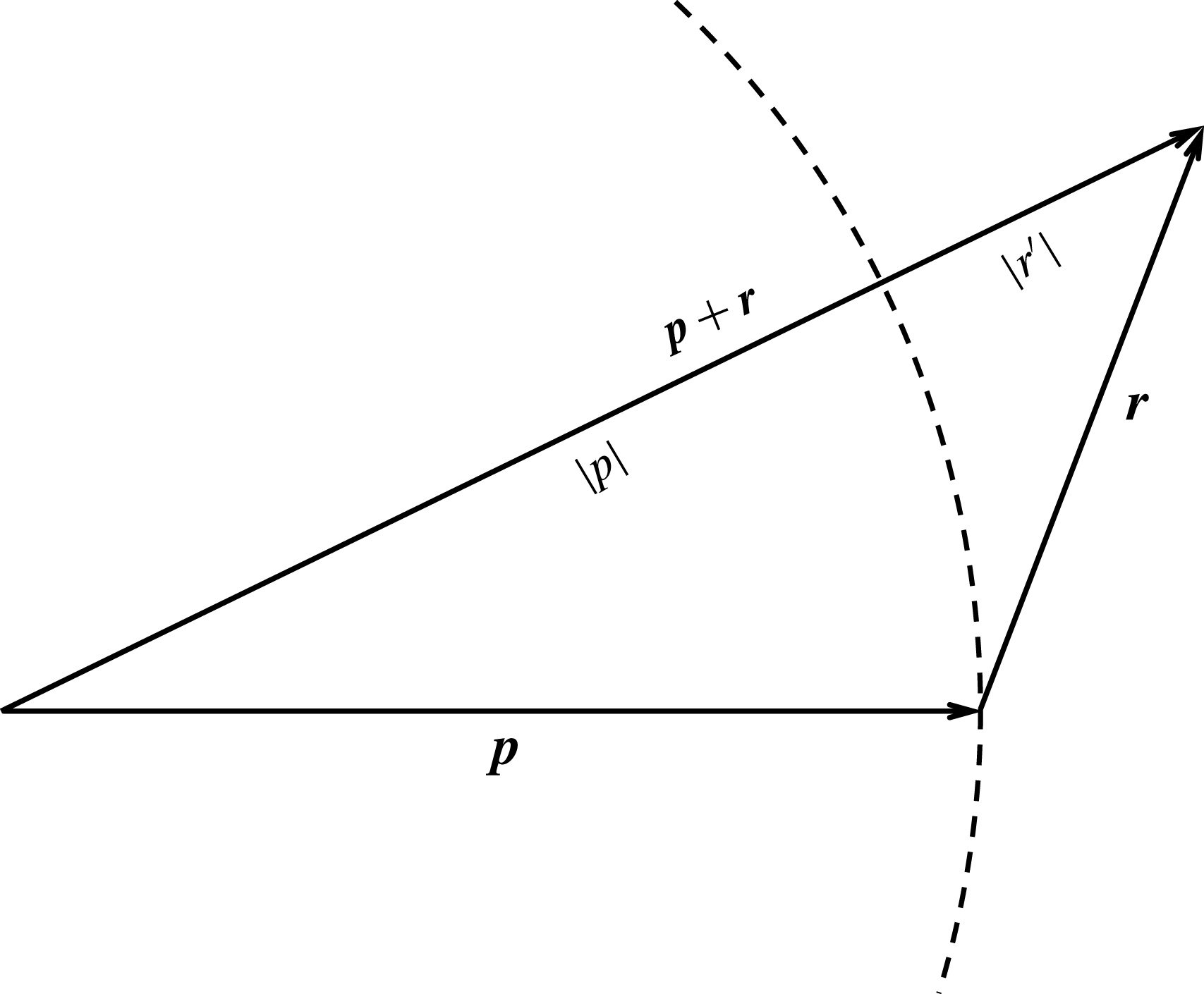
Equation (5.1) is the counterpart of (4.2) in two dimensions, with vectors $\boldsymbol{p}$ and $\boldsymbol{r}$ replacing the scalars $p$ and $r$ (which can be either positive or negative as defined in the one-dimensional proof), and the coefficients $\unicode[STIX]{x1D714}_{\boldsymbol{p}}/k_{\boldsymbol{p}}$ are omitted for simplicity. It can be shown that there exists a (positive or negative) $r^{\prime }\in [-|r|,|r|]$ (see figure 3 for an illustration) such that

(5.2) $$\begin{eqnarray}|\boldsymbol{p}+\boldsymbol{r}|=|p+r^{\prime }|.\end{eqnarray}$$

Figure 3.

Illustration of the existence of $r^{\prime }\in [-|r|,|r|]$ .

With (5.2) substituted into (5.1), $\unicode[STIX]{x1D719}_{z}^{(2)}|_{2D}$ is converted into a scalar form similar to $\unicode[STIX]{x1D719}_{z}^{(2)}$ (cf. 4.2), except that $r$ is now replaced by $r^{\prime }$ . Following the same procedure for $\unicode[STIX]{x1D719}_{z}^{(2)}$ , $\unicode[STIX]{x1D719}_{z}^{(2)}|_{2D}$ can be proved to be free of divergent terms. Since $|r^{\prime }|\leqslant |r|$ , the remaining terms in $\unicode[STIX]{x1D719}_{z}^{(2)}|_{2D}$ after cancellation are bounded by those of  $\unicode[STIX]{x1D719}_{z}^{(2)}$ .

This generalization can be extended to high orders, built on the mathematical induction. For a 2-D surface, equations (4.9) and (4.10) take the form

(5.3) $$\begin{eqnarray}\displaystyle & \unicode[STIX]{x1D702}\hat{D}_{j}\hat{D}_{m}\unicode[STIX]{x1D719}^{s}=\sim {\mathcal{E}}_{\boldsymbol{p},\boldsymbol{q}}^{(j-1)}a_{\boldsymbol{r}}|\boldsymbol{p}|\unicode[STIX]{x1D6FC}_{\boldsymbol{p}}^{(m)}\text{e}^{\text{i}(\boldsymbol{p}+\boldsymbol{q}+\boldsymbol{r})\boldsymbol{\cdot }\boldsymbol{x}}, & \displaystyle\end{eqnarray}$$

(5.4) $$\begin{eqnarray}\displaystyle & \hat{D}_{j}(\unicode[STIX]{x1D702}\hat{D}_{m}\unicode[STIX]{x1D719}^{s})=\sim {\mathcal{E}}_{\boldsymbol{p}+\boldsymbol{r},\boldsymbol{q}}^{(j-1)}a_{\boldsymbol{r}}|\boldsymbol{p}+\boldsymbol{r}|\unicode[STIX]{x1D6FC}_{\boldsymbol{p}}^{(m)}\text{e}^{\text{i}(\boldsymbol{p}+\boldsymbol{q}+\boldsymbol{r})\boldsymbol{\cdot }\boldsymbol{x}}. & \displaystyle\end{eqnarray}$$

Subtraction of (5.4) from (5.3) with the application of (5.2) gives

(5.5) $$\begin{eqnarray}[\unicode[STIX]{x1D702},\hat{D}_{j}]\hat{D}_{m}\unicode[STIX]{x1D719}^{s}=\sim -\text{sgn}(p)[{\mathcal{E}}_{\boldsymbol{ p}+\boldsymbol{r},\boldsymbol{q}}^{(j-1)}\unicode[STIX]{x1D6FC}_{\boldsymbol{p}}^{(m)}(r^{\prime }a_{\boldsymbol{ r}})+({\mathcal{E}}_{\boldsymbol{p}+\boldsymbol{r},\boldsymbol{q}}^{(j-1)}-{\mathcal{E}}_{\boldsymbol{ p},\boldsymbol{q}}^{(j-1)})a_{\boldsymbol{ r}}p\unicode[STIX]{x1D6FC}_{\boldsymbol{p}}^{(m)}]\text{e}^{\text{i}(\boldsymbol{p}+\boldsymbol{q}+\boldsymbol{r})\boldsymbol{\cdot }\boldsymbol{x}}.\end{eqnarray}$$

Since ${\mathcal{E}}_{\boldsymbol{p}+\boldsymbol{r},\boldsymbol{q}}^{(j-1)}\unicode[STIX]{x1D6FC}_{\boldsymbol{p}}^{(m)}(r^{\prime }a_{\boldsymbol{r}})\leqslant O(\unicode[STIX]{x1D716}^{(j+m)})$ with $|r^{\prime }|\leqslant |r|$ , we only need to prove that the second part is free of divergent terms. Following a similar consideration as for (4.7), ${\mathcal{E}}_{\boldsymbol{p},\boldsymbol{q}}^{(j-1)}$ is expressed in vector form as

(5.6) $$\begin{eqnarray}{\mathcal{E}}_{\boldsymbol{p},\boldsymbol{q}}^{(j-1)}=\mathop{\sum }_{\boldsymbol{k}_{1},\ldots ,\boldsymbol{k}_{j-1}}^{\boldsymbol{ k}_{1}+\cdots +\boldsymbol{k}_{j-1}=\boldsymbol{q}}a_{\boldsymbol{ k}_{1}}a_{\boldsymbol{k}_{2}}\ldots a_{\boldsymbol{k}_{j-1}}\mathop{\sum }_{d=1}^{d=d_{0}}c_{d}|\boldsymbol{p}+\boldsymbol{{\mathcal{P}}}_{d,1}||\boldsymbol{p}+\boldsymbol{{\mathcal{P}}}_{d,2}|\ldots |\boldsymbol{p}+\boldsymbol{{\mathcal{P}}}_{d,j-1}|,\end{eqnarray}$$

where $\boldsymbol{{\mathcal{P}}}$ represents the linear combination of $\boldsymbol{k}_{1},\boldsymbol{k}_{2},\ldots ,\boldsymbol{k}_{j-1}$ , with each coefficient being either 0 or 1. This can be converted to the scalar form as

(5.7) $$\begin{eqnarray}{\mathcal{E}}_{\boldsymbol{p},\boldsymbol{q}}^{(j-1)}=\mathop{\sum }_{\boldsymbol{k}_{1},\ldots ,\boldsymbol{k}_{j-1}}^{\boldsymbol{ k}_{1}+\cdots +\boldsymbol{k}_{j-1}=\boldsymbol{q}}a_{\boldsymbol{ k}_{1}}a_{\boldsymbol{k}_{2}}\ldots a_{\boldsymbol{k}_{j-1}}\mathop{\sum }_{d=1}^{d=d_{0}}c_{d}|p+{\mathcal{P}}_{d,1}^{\prime }||p+{\mathcal{P}}_{d,2}^{\prime }|\ldots |p+{\mathcal{P}}_{d,j-1}^{\prime }|,\end{eqnarray}$$

where $p+{\mathcal{P}}^{\prime }$ is the scalar resulting from application of (5.2) (the scenario in figure 3) to each pairwise addition in $|\boldsymbol{p}+\boldsymbol{{\mathcal{P}}}|$ . After eliminating the absolute signs, equation (5.7) results in the polynomial form of $p$ expressed similarly to (4.12).

Similarly, ${\mathcal{E}}_{\boldsymbol{p}+\boldsymbol{r},\boldsymbol{q}}^{(j-1)}$ can be written in scalar form as

(5.8) $$\begin{eqnarray}\displaystyle {\mathcal{E}}_{\boldsymbol{p}+\boldsymbol{r},\boldsymbol{q}}^{(j-1)} & = & \displaystyle \mathop{\sum }_{\boldsymbol{k}_{1},\ldots ,\boldsymbol{k}_{j-1}}^{\boldsymbol{k}_{1}+\cdots +\boldsymbol{k}_{j-1}=\boldsymbol{q}}a_{\boldsymbol{ k}_{1}}a_{\boldsymbol{k}_{2}}\ldots a_{\boldsymbol{k}_{j-1}}\mathop{\sum }_{d=1}^{d=d_{0}}c_{d}|p+{\mathcal{P}}_{d,1}^{\prime }+r_{d,1}^{\prime }||p+{\mathcal{P}}_{d,2}^{\prime }+r_{d,2}^{\prime }|\nonumber\\ \displaystyle & & \displaystyle \ldots |p+{\mathcal{P}}_{d,j-1}^{\prime }+r_{d,j-1}^{\prime }|,\end{eqnarray}$$

where all terms of $r^{\prime }$ are bounded by $[-|r|,|r|]$ .

The subtraction of (5.7) from (5.8) for sufficiently small $|r|$ follows that in § 4.2, except that the term $(p+r)^{i}-p^{i}$ is replaced by $(p+r_{1}^{\prime })(p+r_{2}^{\prime })\ldots (p+r_{i}^{\prime })-p^{i}$ . The latter is bounded by

(5.9) $$\begin{eqnarray}\displaystyle & & \displaystyle p^{i}\mathop{\sum }_{n=1}^{i}\binom{i}{n}(-|r/p|)^{n}\leqslant (p+r_{1}^{\prime })(p+r_{2}^{\prime })\ldots (p+r_{i}^{\prime })-p^{i}\leqslant p^{i}\mathop{\sum }_{n=1}^{i}\binom{i}{n}|r/p|^{n},\nonumber\\ \displaystyle & & \displaystyle \quad \text{for}~i=1,2,\ldots ,j-1,\end{eqnarray}$$

and the two bounds can both be proved to result in the cancellation of all divergent terms. The remaining proof for general $r$ follows in a straightforward manner as in § 4.2. The difference ${\mathcal{E}}_{\boldsymbol{p},\boldsymbol{q}}^{(j-1)}-{\mathcal{E}}_{\boldsymbol{p}+\boldsymbol{r},\boldsymbol{q}}^{(j-1)}$ , after splitting into a finite number of subintervals, can again be shown to be bounded by $O(\unicode[STIX]{x1D716}^{j-1}|r/p|)$ . The final result is that $[\unicode[STIX]{x1D702},\hat{D}_{j}]\hat{D}_{m}\unicode[STIX]{x1D719}^{s}$ is free of divergent terms, and $\unicode[STIX]{x1D719}_{z}^{(m)}\sim O(\unicode[STIX]{x1D716}^{m})$ for all integer $m$ for a 2-D surface. We thus generalize the proof of cancellation of divergent terms from 1-D to 2-D surfaces.

6 Conclusion and discussion

We consider the perturbation expansion solution $\unicode[STIX]{x1D719}_{z}=\sum _{m=1}^{M}\unicode[STIX]{x1D719}_{z}^{(m)}$ , given $\unicode[STIX]{x1D702}$ and $\unicode[STIX]{x1D719}^{s}$ , for a multi-scale wave field with significantly disparate wavelengths. The goal is to quantify the influence of divergent terms of the form $O(k_{S}a_{L})$ on the convergence of the expansion. We first illustrate numerically that these divergent terms are subject to cancellation at each order, but a numerical ill-conditioning eventually occurs at some $M>M_{d}$ depending on the machine precision. This is due to the roundoff error of the floating point representation of the divergent terms that cannot be avoided in a typical pseudo-spectral approach using fast transforms such as HOS. The cancellation of divergent terms is then studied theoretically, starting from consideration of a one-dimensional surface. Retaining the modal decomposition framework and considering a pair of long–short wave modes, we extend existing result to $m=3$ . The generalization of this to higher order $m>3$ involving an exponentially increasing number of interaction terms (even for two modes) is practically untenable. To circumvent this, we provide a general proof based on mathematical induction, using Dirichlet–Neumann operators, showing analytical cancellation of the divergent terms at arbitrary order $m$ for multi-scale broadband waves. We thus show that the expansion of $\unicode[STIX]{x1D719}_{z}$ is bounded by the power series of the small parameter of modal wave steepness $\unicode[STIX]{x1D716}$ , and $\unicode[STIX]{x1D719}_{z}^{(m)}\sim O(\unicode[STIX]{x1D716}^{m})$ , which is consistent with the numerical illustration. The proof is finally extended to general two-dimensional surfaces.

The demonstration of numerical ill-conditioning and the proof of the analytical cancellation of the divergent terms suggest the need and opportunity for alternative approaches that avoid this difficulty for nonlinear long–short wave interaction simulations. One useful class of approaches is based on transformation of variables mapping the wavy free surface to a horizontal plane, e.g. Nicholls & Reitich (Reference Nicholls and Reitich2001) (see also particular implementations for water wave problems, e.g. Nicholls Reference Nicholls2007, Reference Nicholls2009; Pan Reference Pan2016). The ill conditioning is in principle avoided but the computational effort is substantially increased with the loss of the dimension-reduction property of methods such as HOS. The analytical cancellation of the divergent terms at any order suggests an alternative within the framework of HOS. Instead of calculating products in the physical domain, we perform all operations using modal convolution in the spectral domain and store the results only after the analytical cancellations demonstrated in § 4.1. This avoids the numerical ill-conditioning and retains the dimension-reduction property in principle, but results in much higher computational complexity due to the computation of modal convolution, and the generalization of the algorithm to general $m$ is not straightforward.