1 Introduction
The processes by which shear at the surface of a stably stratified body of fluid mixes and deepens the upper portions of the fluid body play an important role in the dynamics of many situations of interest, such as in lakes and oceans as well as in many industrial flows (Turner Reference Turner1979; Fernando Reference Fernando1991; Stevens & Imberger Reference Stevens and Imberger1996; Ivey, Winters & Koseff Reference Ivey, Winters and Koseff2008). In general, mixing and turbulence tend to be suppressed when the fluid is sufficiently stably stratified, however when shear stress and buoyancy stratification are roughly in balance, the resultant dynamics can be quite complicated (Sherman, Imberger & Corcos Reference Sherman, Imberger and Corcos1978; Majda & Shefter Reference Majda and Shefter2000; Peltier & Caulfield Reference Peltier and Caulfield2003).
The situation where an unsteady well-mixed region is separated from a stably stratified region is a common occurrence in many geophysical and astrophysical settings, and there continues to be intense interest in these flows, particularly in regards to the mechanisms by which energy and possibly momentum from the well-mixed region can be transported deep into the stratified region. Internal wave beams are a leading candidate and it is of much interest to understand how these are generated (Michaelian, Maxworthy & Redekopp Reference Michaelian, Maxworthy and Redekopp2002; Dohan & Sutherland Reference Dohan and Sutherland2003; Pham, Sarkar & Brucker Reference Pham, Sarkar and Brucker2009; Ansong & Sutherland Reference Ansong and Sutherland2010; Munroe & Sutherland Reference Munroe and Sutherland2014).
Our understanding of the processes involved is still quite limited. A useful analogue problem that is relatively straightforward to produce as a laboratory experiment and to simulate numerically is the lid-driven stratified cavity flow. Many studies exist in cavities with various aspect ratios or shapes, driven at one or more walls, with a temperature gradient either in the direction opposite to gravity (stable stratification), the perpendicular direction (horizontal convection) or in the same direction (Rayleigh–Bénard convection), in various media (air, water, oils, with different Prandtl numbers
 $\mathit{Pr}$
), or in the presence of internal obstacles or fins. However, relatively few studies have explored the flow behaviour over a comprehensive range of the Reynolds and Richardson numbers,
 $\mathit{Re}$
and
 $\mathit{Ri}$
, characterising the shear and buoyancy of the flow regime. Such a comprehensive study is the goal of the present numerical investigation.
Most studies of the stably stratified configuration used here (where side walls are insulated and the top and bottom walls are kept at fixed temperatures) have been limited to relatively low Grashof numbers,
 $\mathit{Gr}=\mathit{Ri}\,\mathit{Re}^{2}\lesssim O(10^{6})$
, normally associated (for moderate
 $\mathit{Pr}$
) with steady state responses (Iwatsu, Hyun & Kuwahara Reference Iwatsu, Hyun and Kuwahara1993; Nicolás & Bermúdez Reference Nicolás and Bermúdez2005; Cheng & Liu Reference Cheng and Liu2010), in some cases as part of a more general investigation of doubly diffusive (temperature and solute) systems (Maiti, Gupta & Bhattacharyya Reference Maiti, Gupta and Bhattacharyya2008). The experimental study of Koseff & Street (Reference Koseff and Street1985) in a three-dimensional cavity with aspect ratio 1 : 3 : 1 (square vertical cross-section) filled with water (
 $\mathit{Pr}\approx 7$
) remains the quintessential reference for flows at large
 $\mathit{Gr}\sim O(10^{7}{-}10^{8})$
. Their visualisations in the (vertical) symmetry plane provide some general understanding of the competition between shear and buoyancy forces in regimes where the flows are expected to be unsteady, but they only present transient dynamics (the longest experiment corresponds to
 $t\approx 0.3$
viscous times). Ji, Kim & Hyun (Reference Ji, Kim and Hyun2007) provide experimental and numerical evidence of oscillatory behaviour at large
 $\mathit{Re}$
and moderate
 $\mathit{Ri}$
in air (
 $\mathit{Pr}\approx 0.7$
), but they only report on the vertical temperature distribution. Blanchette, Peacock & Cousin (Reference Blanchette, Peacock and Cousin2008) used salt stratification (
 $\mathit{Pr}\approx 600$
) to investigate the relationship between the Péclet number
 $\mathit{Pe}=\mathit{Re}\,\mathit{Pr}$
and the Rayleigh number
 $\mathit{Ra}=\mathit{Gr}\,\mathit{Pr}$
at the onset of instability of the steady flow, using the synthetic schlieren technique, at large
 $\mathit{Ri}$
(with
 $\mathit{Gr}\sim O(10^{10}{-}10^{12})$
) and obtained good agreement with their two-dimensional stability analysis. Cohen et al. (Reference Cohen, Eidelman, Elperin, Kleerin and Rogachevskii2014) investigated stably stratified air flow in experiments in a three-dimensional lid-driven cavity in the large
 $\mathit{Re}$
and small
 $\mathit{Ri}$
regime, presenting mean flow features and statistics of the turbulent flow. Consistent with the previous studies, they observed the buoyant confinement of the lid-driven roller to the upper downstream corner. They also presented some scaling analysis of the unsteady flow, but gave few details of the unsteadiness or how it comes about. They found that the flow is not strongly three-dimensional, particularly as the stratification is increased, with the mean kinetic energy in the spanwise flow component being at least ten times weaker than in the streamwise component. This motivates us to do a detailed numerical investigation of the onset and the dynamics of the unsteady flow.
The results of the present study in the two-dimensional square cavity in the low-
 $\mathit{Re}$
regime (
 $\mathit{Re}\lesssim 1000$
) confirm previous results and observations of steady state solutions and validate our numerical approach. A detailed study of the instability of the steady state as
 $\mathit{Re}$
is increased is carried out over a large range in
 $\mathit{Ri}$
. Details of the bifurcating unsteady states are analysed using a bifurcation theoretic approach and frequency analyses of flow kinetic energy, revealing an intricate pattern of responses due to competition between buoyancy and inertial effects.
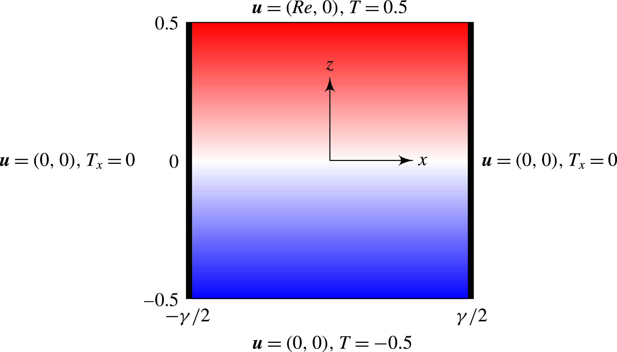
Schematic of the system, indicating the non-dimensional coordinate system and boundary conditions. The top boundary moves to the right (positive
 $x$
direction) at constant speed
 $\mathit{Re}$
. The colour map shows the linearly stratified temperature distribution (red is
 $T=0.5$
, blue is
 $T=-0.5$
and white is
 $T=0$
) when
 $\mathit{Re}=0$
.

2 Governing equations
Consider the flow in a rectangular cavity of depth
 $d$
and width
 $l$
, filled with a fluid of kinematic viscosity
 $\unicode[STIX]{x1D708}$
, thermal diffusivity
 $\unicode[STIX]{x1D705}$
and coefficient of volume expansion
 $\unicode[STIX]{x1D6FD}$
. The top boundary of the cavity is driven horizontally at a constant speed
 $U$
and is maintained at a fixed temperature
 $T_{top}$
. The bottom boundary is maintained at a cooler fixed temperature
 $T_{bot}$
, whilst the two side walls are insulated. Gravity
 $g$
acts in the downward vertical direction. We consider the two-dimensional problem here as it allows for an extensive parameter study. This is also in part motivated by the observation that the dominant modes of linearised instability for stratified shear flows are two-dimensional (Majda & Shefter Reference Majda and Shefter1998). The temperature deviation from the mean temperature,
 $(T_{top}+T_{bot})/2$
, is non-dimensionalised with
 $\unicode[STIX]{x0394}T=T_{top}-T_{bot}$
. Figure 1 shows a schematic of the system. Using
 $d$
as the length scale and the viscous time
 $d^{2}/\unicode[STIX]{x1D708}$
as the time scale, the non-dimensional governing equations, employing the Boussinesq approximation, are
 $$\begin{eqnarray}\left.\begin{array}{@{}c@{}}\displaystyle \boldsymbol{u}_{t}+\boldsymbol{u}\boldsymbol{\cdot }\unicode[STIX]{x1D735}\boldsymbol{u}=-\unicode[STIX]{x1D735}p+\unicode[STIX]{x1D6FB}^{2}\boldsymbol{u}+\mathit{Gr}\,T\boldsymbol{e}_{z},\quad \unicode[STIX]{x1D735}\boldsymbol{\cdot }\boldsymbol{u}=0,\\ \displaystyle T_{t}+\boldsymbol{u}\boldsymbol{\cdot }\unicode[STIX]{x1D735}T=\frac{1}{\mathit{Pr}}\unicode[STIX]{x1D6FB}^{2}T.\end{array}\right\}\end{eqnarray}$$
The boundary conditions are:
 $$\begin{eqnarray}\left.\begin{array}{@{}c@{}}\text{top, }(x,z)=(x,0.5):\quad (u,w,T)=(\mathit{Re},0,0.5),\\ \text{bottom, }(x,z)=(x,-0.5):\quad (u,w,T)=(0,0,-0.5),\\ \text{sides, }(x,z)=(\pm 0.5\unicode[STIX]{x1D6FE},z):\quad (u,w,T_{x})=(0,0,0),\end{array}\right\}\end{eqnarray}$$
where
 $\unicode[STIX]{x1D6FE}=l/d$
is the aspect ratio.
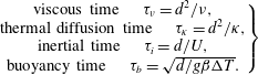
There are four time scales of relevance; these are
 $$\begin{eqnarray}\left.\begin{array}{@{}c@{}}\text{viscous time }\quad \unicode[STIX]{x1D70F}_{\unicode[STIX]{x1D708}}=d^{2}/\unicode[STIX]{x1D708},\\ \text{thermal diffusion time }\quad \unicode[STIX]{x1D70F}_{\unicode[STIX]{x1D705}}=d^{2}/\unicode[STIX]{x1D705},\\ \text{inertial time }\quad \unicode[STIX]{x1D70F}_{i}=d/U,\\ \text{buoyancy time }\quad \unicode[STIX]{x1D70F}_{b}=\sqrt{d/g\unicode[STIX]{x1D6FD}\unicode[STIX]{x0394}T}.\end{array}\right\}\end{eqnarray}$$
The governing parameters can be expressed as ratios of these time scales:
 $$\begin{eqnarray}\left.\begin{array}{@{}c@{}}\text{Prandtl number }\quad \mathit{Pr}=\unicode[STIX]{x1D70F}_{\unicode[STIX]{x1D705}}/\unicode[STIX]{x1D70F}_{\unicode[STIX]{x1D708}}=\unicode[STIX]{x1D708}/\unicode[STIX]{x1D705},\\ \text{Reynolds number }\quad \mathit{Re}=\unicode[STIX]{x1D70F}_{\unicode[STIX]{x1D708}}/\unicode[STIX]{x1D70F}_{i}=Ud/\unicode[STIX]{x1D708},\\ \text{Richardson number }\quad \mathit{Ri}=(\unicode[STIX]{x1D70F}_{i}/\unicode[STIX]{x1D70F}_{b})^{2}=g\unicode[STIX]{x1D6FD}\unicode[STIX]{x0394}Td/U^{2},\\ \text{Grashof number }\quad \mathit{Gr}=(\unicode[STIX]{x1D70F}_{\unicode[STIX]{x1D708}}/\unicode[STIX]{x1D70F}_{b})^{2}=\mathit{Ri}\mathit{Re}^{2}=\unicode[STIX]{x1D6FD}gd^{3}\unicode[STIX]{x0394}T/\unicode[STIX]{x1D708}^{2}.\end{array}\right\}\end{eqnarray}$$
In this study
 $\unicode[STIX]{x1D6FE}=1$
and
 $\mathit{Pr}=1$
, and we consider variations in the independent parameters
 $\mathit{Re}$
and
 $\mathit{Ri}$
.
3 Numerical method
The governing equations (2.1) are discretised using a spectral-collocation method in both spatial directions. Both velocity components and pressure are approximated by Chebyshev polynomials of the first kind with degree less than
 $M$
, associated with the Chebyshev–Gauss–Lobatto grid. Spatial differentiation is performed via direct matrix-vector multiplication by the pseudo-spectral differentiation matrix.
The boundary condition for the
 $x$
-velocity at the moving top wall,
 $u(x,0.5)=\mathit{Re}$
, is discontinuous where it meets the two vertical side walls, which can lead to Gibbs phenomena when using a global spectral method. In order to resolve this numerical issue, we regularise the top wall boundary condition by using:
 $$\begin{eqnarray}u(x,0.5)=\mathit{Re}[1-\exp (-(1-4x^{2})/\unicode[STIX]{x1D6FF})].\end{eqnarray}$$
The small positive number
 $\unicode[STIX]{x1D6FF}$
controls the distance over which the discontinuity is regularised. For the results presented here, we have used
 $\unicode[STIX]{x1D6FF}=0.03$
. Smaller values of
 $\unicode[STIX]{x1D6FF}$
, corresponding to narrower gaps between the top lid and the vertical sides, lead to qualitatively similar results while significantly increasing the computational demand.
For the smaller
 $\mathit{Re}$
and
 $\mathit{Ri}$
values considered, a collocation grid with
 $M=128$
points in each direction provides sufficiently many points in the regularisation regions near the top corners to yield reliable results. For larger
 $\mathit{Re}$
and
 $\mathit{Ri}$
, finer grids were used, with
 $M=196$
being used for the largest
 $\mathit{Re}$
and
 $\mathit{Ri}$
in order to resolve the flows.
The time integration scheme used is the fractional-step improved projection method of Hugues & Randriamampianina (Reference Hugues and Randriamampianina1998), based on a linearly implicit and stiffly stable second-order accurate scheme, combining a backward differentiation formula for the linear terms and an implicit mix, equivalent to linear extrapolation, of Adams–Moulton and Adams–Bashforth steps for the nonlinear advective terms (Vanel, Peyret & Bontoux Reference Vanel, Peyret, Bontoux, Morton and Baines1986). The predictor stage of the fractional step method solves a Helmholtz equation for a pressure field, for which Neumann conditions consistent with (2.1) are applied at the walls. The corrector stage then projects the resulting predicted velocity field onto the space of (discretely) divergence-free polynomials via a Stokes problem, which is also handled by solving a Helmholtz equation for the corrected pressure, albeit with homogeneous Neumann boundary conditions. The code used in the present study is essentially the same as that used in Lopez et al. (Reference Lopez, Welfert, Wu and Yalim2017), but restricted to two-dimensional flow, and augmented with the temperature equation and the buoyancy term in the momentum equation.
Depending on the values of
 $\mathit{Re}$
and
 $\mathit{Ri}$
, one or multiple solutions can be obtained from different initial conditions, such as steady state (S), limit cycles (L) or quasi-periodic states (QP) which are mixed modes of limit cycles whose frequencies may or may not be commensurate, and in some parameter regimes even more temporally complicated states exist. In general, the initial condition used is the static linearly stratified state, i.e.
 $u=w=0$
and
 $T=z$
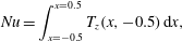
. Other solutions can be obtained via continuation using solutions from nearby parameter values as initial conditions. To determine the type of solution, we monitor two global indicators of the flow: the non-dimensional heat flux through the bottom wall of the cavity (Nusselt number)
 $$\begin{eqnarray}\mathit{Nu}=\int _{x=-0.5}^{x=0.5}T_{z}(x,-0.5)\,\text{d}x,\end{eqnarray}$$
and the total kinetic energy
 $$\begin{eqnarray}\mathit{E}=\frac{1}{\mathit{Re}^{2}}\int _{z=-0.5}^{z=0.5}\int _{x=-0.5}^{x=0.5}(u^{2}+w^{2})\,\text{d}x\,\text{d}z.\end{eqnarray}$$
In general,
 $\mathit{Nu}\geqslant 1$
(with
 $\mathit{Nu}=1$
for the static state, which only exists at
 $\mathit{Re}=0$
), and
 $\mathit{E}<1$
. Note that for steady states,
 $\mathit{Nu}$
also corresponds to the heat flux through the top boundary, whereas for unsteady states, the heat flux through the top and the bottom are not necessarily the same at any instant in time, but their long-time averages converge to the same value.
Unsteady flows are characterised by their temporal frequencies,
 $f$
, obtained from the power spectral density (PSD) of the time series (which is first trimmed, de-trended, and Blackman filtered) of the kinetic energy
 $\mathit{E}$
. Since the flows are computed using the viscous time scale, the frequencies can vary widely with
 $\mathit{Re}$
and
 $\mathit{Ri}$
. In order to compare values of
 $f$
over a large range of
 $\mathit{Re}$
and
 $\mathit{Ri}$
, we use the scaled angular frequency
 $$\begin{eqnarray}F=\frac{f}{\sqrt{\mathit{Re }^{2}+\mathit{ Gr}}}=\frac{f}{\mathit{Re}\sqrt{1+\mathit{ Ri}}}.\end{eqnarray}$$
This scaling reduces the measure
 $f$
in the viscous time scale to the measure
 $F$
of the frequency in the inertial time scale when
 $\mathit{Gr}=0$
with
 $\mathit{Re}\neq 0$
fixed (i.e.
 $\mathit{Ri}=0$
) and to the measure
 $F$
in the buoyancy time scale when
 $\mathit{Re}=0$
with
 $\mathit{Gr}\neq 0$
fixed (i.e.
 $\mathit{Ri}\rightarrow \infty$
), thus providing a smooth transition between these time scales for intermediate
 $\mathit{Ri}$
values. Plots of the PSDs obtained for fixed
 $\mathit{Re}$
but different
 $\mathit{Ri}$
are normalised using the global peak power to reflect relative signal strengths, with the colour scale ranging from white (
 $-50$
dB, corresponding to
 $10^{-5}$
power) to black (0 dB, associated with unit peak power).
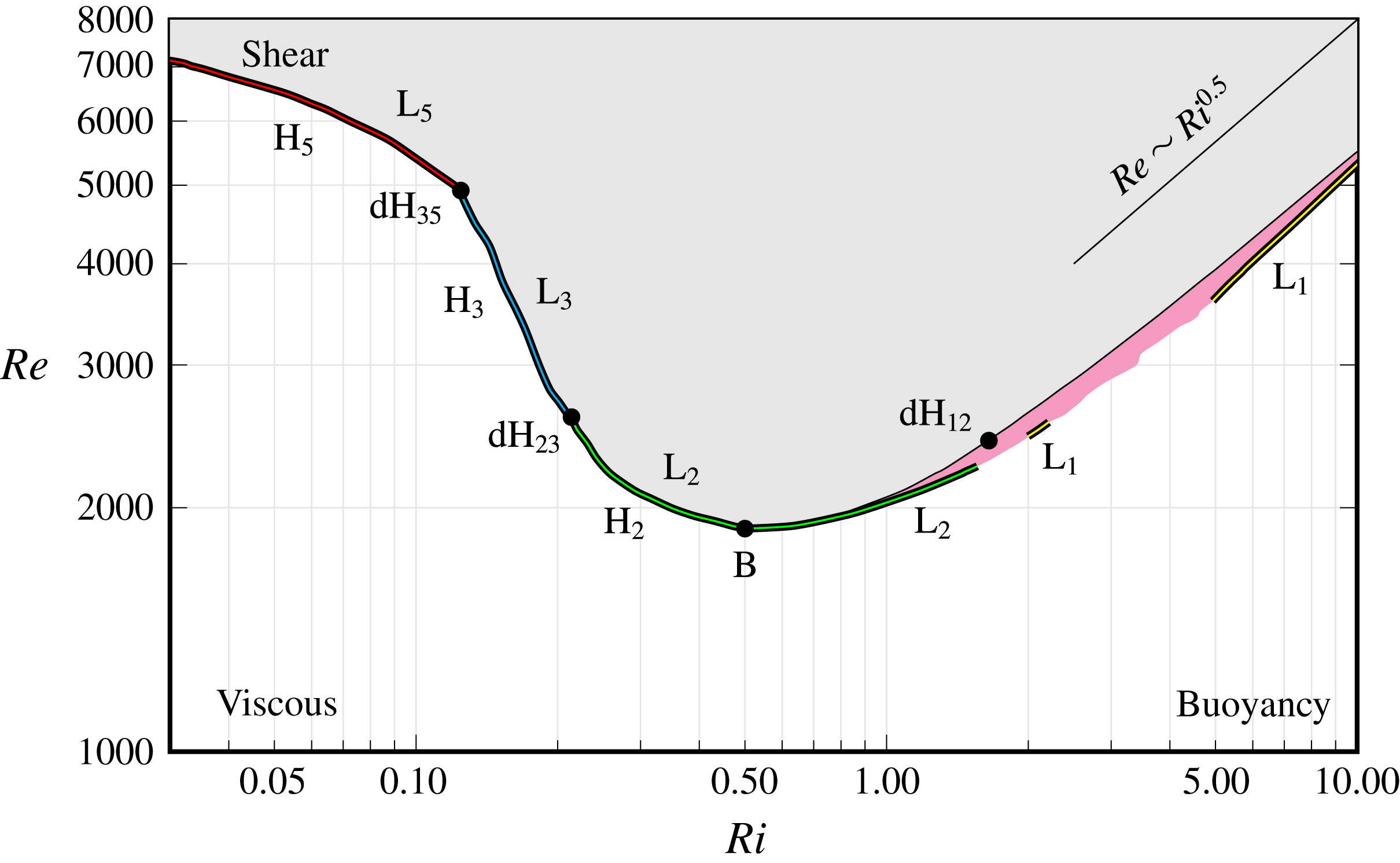
Phase diagram in the
 $(\mathit{Ri},\mathit{Re})$
parameter space. Below the Hopf bifurcation curves, H
 $_{i}$
with
 $i=2$
, 3 and 5, only the steady state, S, exists and is stable. Above the Hopf bifurcation curves, unsteady states including the limit cycles L
 $_{i}$
with
 $i=1$
, 2, 3 and 5, exist in the grey shaded region. The dynamics in the magenta shaded region is hysteretic, with S and unsteady states attracting. Codimension-two points where two different Hopf bifurcation curves meet are indicated with bullets for the double-Hopf points dH
 $_{35}$
, dH
 $_{23}$
and dH
 $_{12}$
, as well as the Bautin point B where the Hopf bifurcation H
 $_{2}$
changes from being supercritical to subcritical.
4 Results
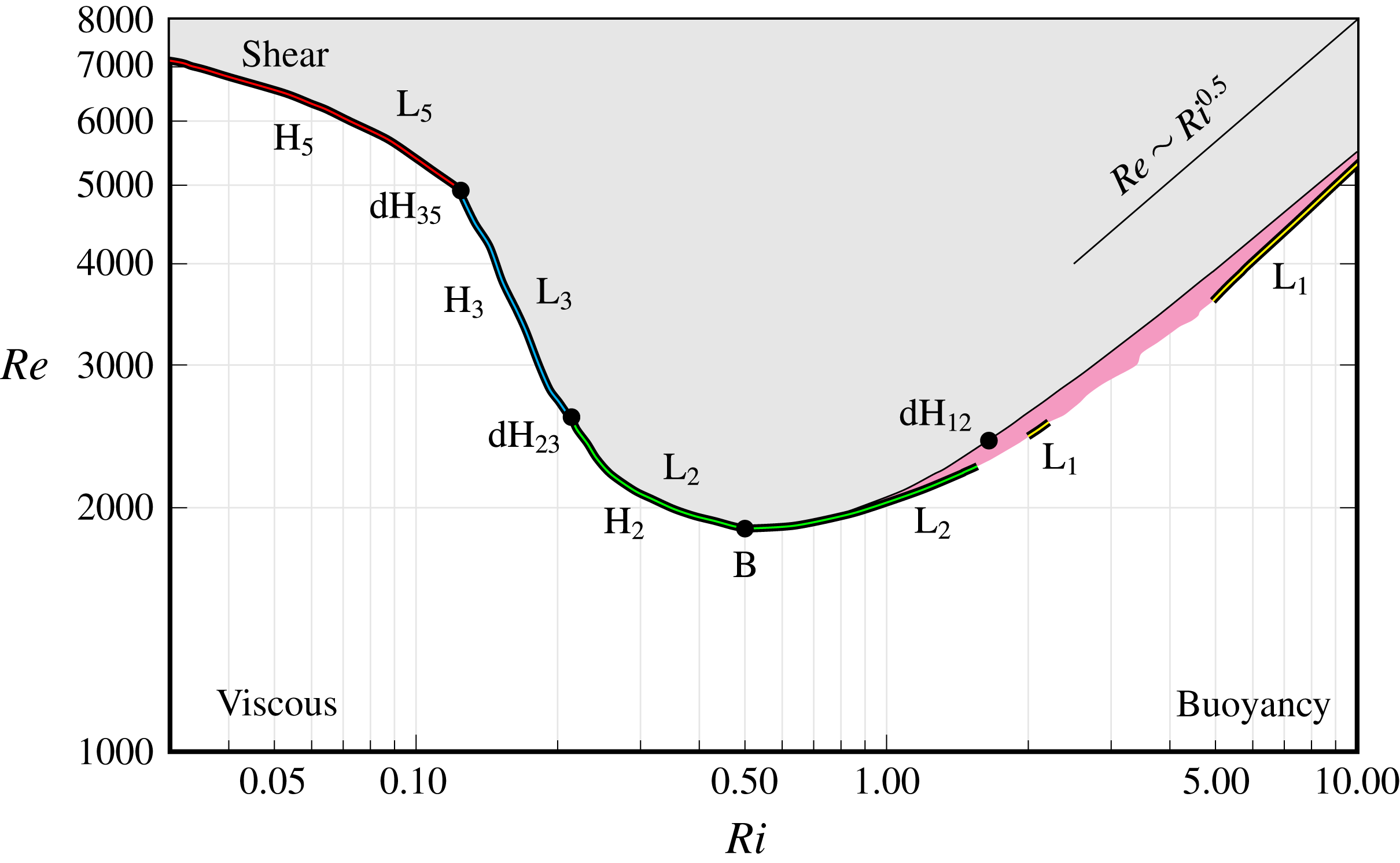
Figure 2 provides a global overview of the regions in the
 $(\mathit{Ri},\mathit{Re})$
parameter space where either the steady base state S is the only observed response (unshaded region), or sustained unsteady responses are observed (shaded regions). For fixed
 $\mathit{Ri}$
, S is observed at low
 $\mathit{Re}$
, for which viscous effects are dominant. At larger
 $\mathit{Re}$
, competing shear and buoyancy effects destabilise S and lead to various time-dependent states. In the following subsections, we describe the bifurcations that result in these unsteady states and their nonlinear dynamics.
4.1 Steady state at low
 $\mathit{Re}$
numbers

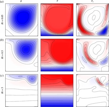
Streamlines
 $\unicode[STIX]{x1D713}$
, isotherms
 $T$
and horizontal temperature gradient
 $T_{x}$
of S at
 $\mathit{Re}=1000$
and
 $\mathit{Ri}$
as indicated. The contour levels are equispaced in ranges
 $|\unicode[STIX]{x1D713}|\leqslant 100$
,
 $|T|\leqslant 0.5$
, and
 $|T_{x}|\leqslant 1.5$
.
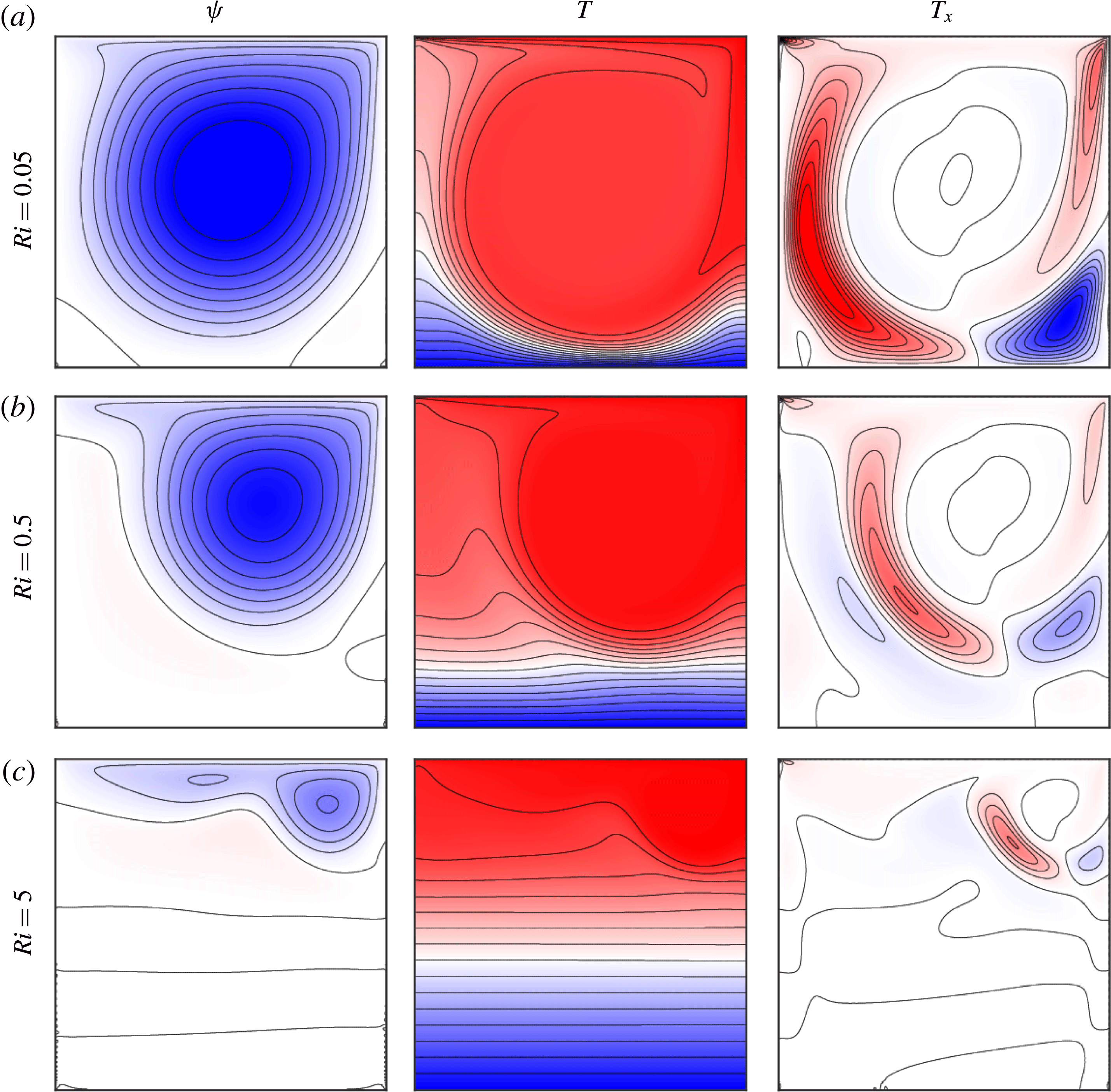
For small enough
 $\mathit{Re}$
, the flow evolves to a steady state S for all values of
 $\mathit{Ri}$
. Figure 3 show streamlines and temperature contours of S for
 $\mathit{Ri}=0.05$
,
 $0.5$
and
 $5$
at
 $\mathit{Re}=1000$
. The streamlines are the isocontours of the streamfunction
 $\unicode[STIX]{x1D713}$
, where
 $(u,w)=(\unicode[STIX]{x1D713}_{z},-\unicode[STIX]{x1D713}_{x})$
. The horizontal temperature gradient
 $T_{x}$
, which is a source of vorticity, provides all the essential information on the dynamics of the flow and is also included in figure 3; it will be the main quantity of interest at higher
 $\mathit{Re}$
values.
For
 $\mathit{Ri}\ll 0.5$
, shear effects dominate over buoyancy effects, resulting in full vertical penetration of the lid-driven roller and temperature homogenisation throughout most of the cavity. This leads to a steep temperature gradient at the bottom of the cavity (see figure 3
a for
 $\mathit{Ri}=0.05$
). The presence of two weak secondary recirculation zones at the bottom corners is consistent with the flow in the isothermal lid-driven cavity (Koseff & Street Reference Koseff and Street1985; Iwatsu et al.
Reference Iwatsu, Hyun and Kuwahara1993; Nicolás & Bermúdez Reference Nicolás and Bermúdez2005). The impact of the non-isothermal conditions is that in the core of the main roller, the temperature is essentially uniformly hot and it is inside this roller where the streamfunction has non-zero gradients (i.e. there is a meridional circulation). The lid-driven roller is delineated by regions of large horizontal temperature gradients
 $T_{x}$
separating the isothermal overturning flow in the roller from the temperature-stratified near-static fluid outside the roller.
For
 $\mathit{Ri}\approx 0.5$
, buoyancy and shear effects are of comparable strength and their competition results in a smaller roller restricted toward the downstream top corner and a deeper stratification zone in the bottom of the cavity (see figure 3
b for
 $\mathit{Ri}=0.5$
). Since advection brings the temperature at the top of the stratification zone in line with the temperature at the top of the cavity, the temperature gradient through the bottom stratified region is lower than it is at smaller
 $\mathit{Ri}$
. These features are consistent with the numerical results in Iwatsu et al. (Reference Iwatsu, Hyun and Kuwahara1993).
For
 $\mathit{Ri}\gg 0.5$
, buoyancy confines the roller to the upper right corner of the cavity, and the flow is essentially unable to penetrate into the stratified zone. The streamlines indicate a number of very weak horizontal recirculation layers in the stratified zone. In the example shown in figure 3(c) for
 $\mathit{Ri}=5$
, there are four such layers. For different
 $\mathit{Re}$
and
 $\mathit{Ri}$
, different numbers of similar layers have been reported (Koseff & Street Reference Koseff and Street1985; Nicolás & Bermúdez Reference Nicolás and Bermúdez2005).
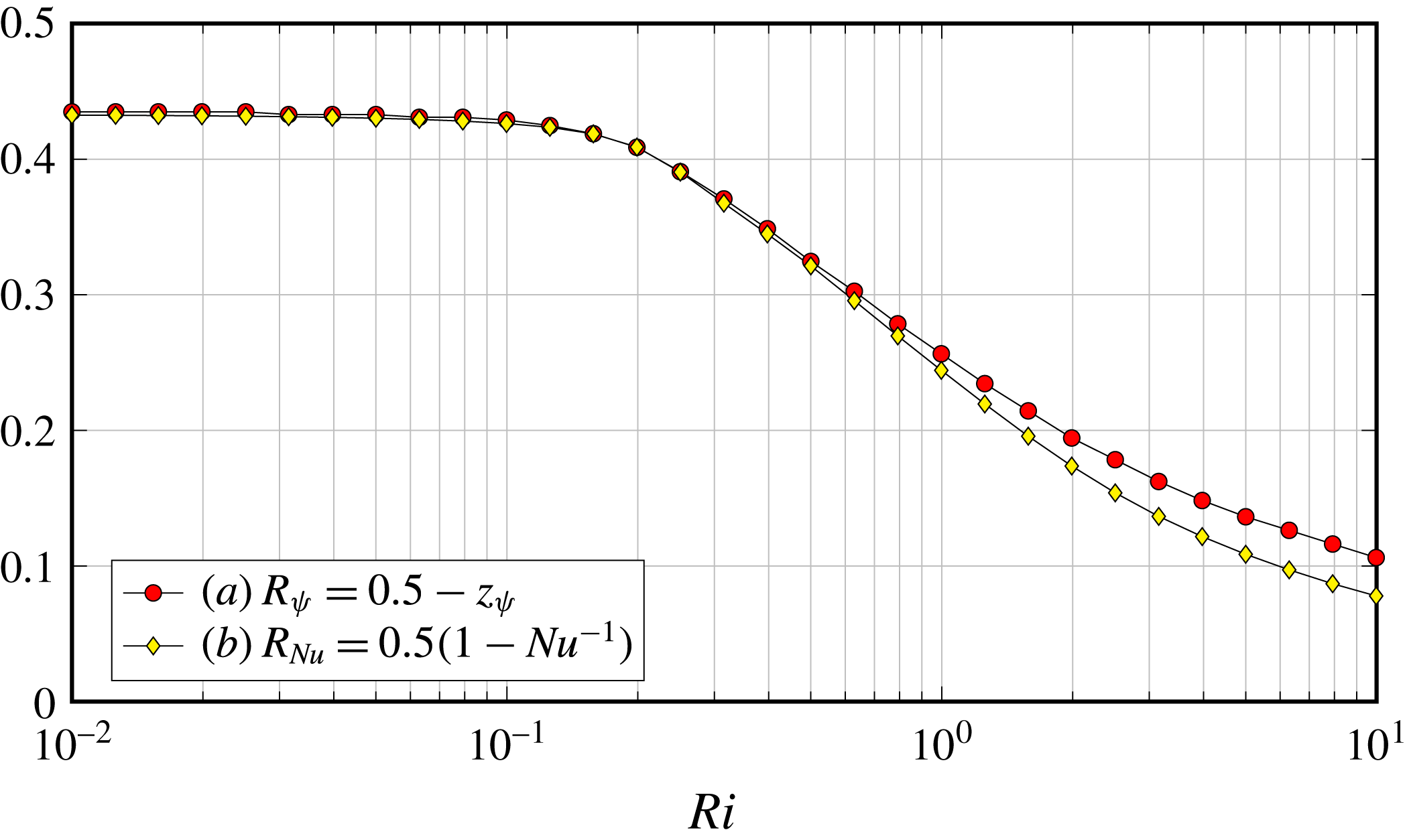
Radius of the primary roller as a function of
 $\mathit{Ri}$
at
 $\mathit{Re}=1000$
, estimated from the vertical position
 $z_{\unicode[STIX]{x1D713}}$
of the streamfunction minimum, and the Nusselt number
 $\mathit{Nu}$
.
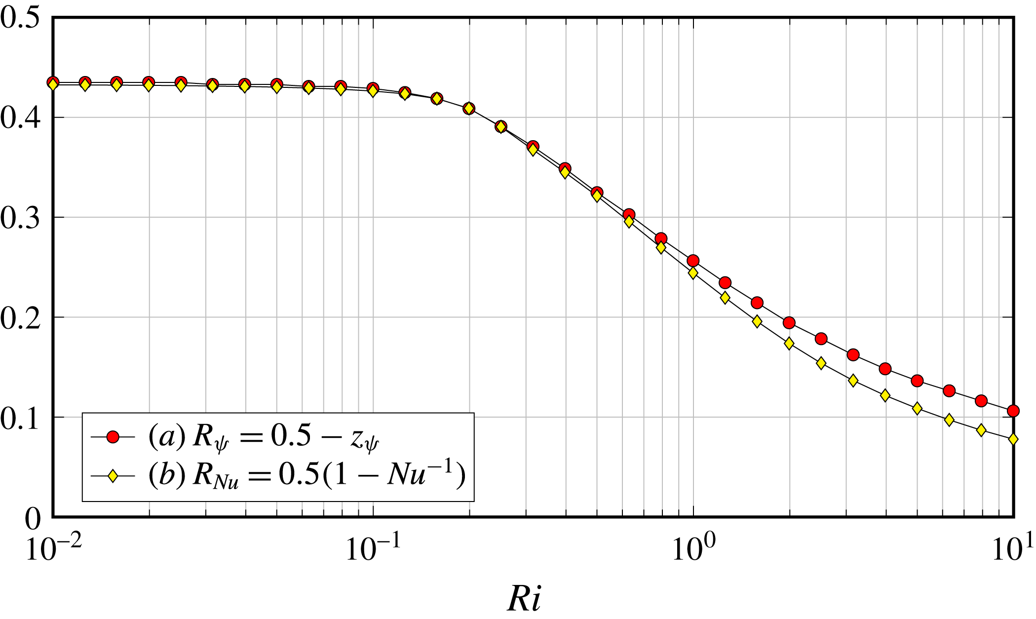
The radius of the lid-driven roller can be estimated from the vertical position
 $z_{\unicode[STIX]{x1D713}}$
of the minimum of the streamfunction
 $\unicode[STIX]{x1D713}$
, by assuming a perfectly circular roller, namely
 $R_{\unicode[STIX]{x1D713}}\approx 0.5-z_{\unicode[STIX]{x1D713}}$
. Alternately, the radius can be estimated from
 $\mathit{Nu}\approx 1/(1-2R_{\mathit{Nu}})$
by assuming a constant vertical temperature gradient below a roller of radius
 $R_{\mathit{Nu}}$
and a uniform temperature within the roller. These assumptions are supported by figure 3(b). The two estimates of the radius,
 $R_{\unicode[STIX]{x1D713}}$
and
 $R_{\mathit{Nu}}$
, are shown in figure 4 for
 $\mathit{Re}=1000$
and
 $\mathit{Ri}\in [0.01,10]$
. The two roller radii estimates are similar, especially for
 $\mathit{Ri}\lesssim 0.5$
. Both estimates decrease with increasing
 $\mathit{Ri}$
for
 $\mathit{Ri}\gtrsim 0.2$
, with the roller depth
 $2R_{\unicode[STIX]{x1D713}}$
or
 $2R_{\mathit{Nu}}$
being approximately two thirds the depth of the cavity at
 $\mathit{Ri}=0.5$
, and one half at
 $\mathit{Ri}=1$
. These results are also qualitatively similar to those measured experimentally by Cohen et al. (Reference Cohen, Eidelman, Elperin, Kleerin and Rogachevskii2014, figure 6).
4.2 Instability of S for
$\mathit{Ri}<0.5$
: supercritical Hopf bifurcations

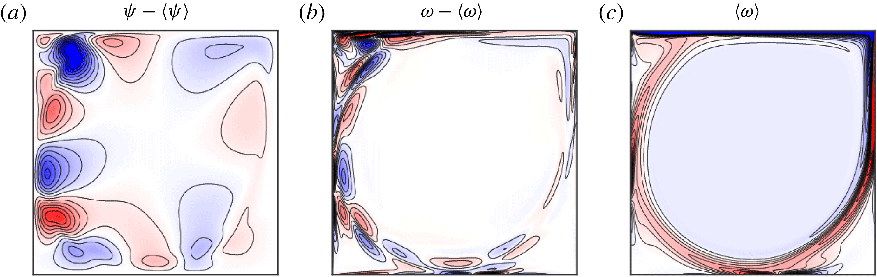
Snapshots of the deviations from the time averages of (a) the streamfunction, (b) vorticity and
 $(c)$
the time-averaged vorticity, for the limit cycle L
 $_{5}$
at
 $\mathit{Re}=8016$
and
 $\mathit{Ri}=0$
.
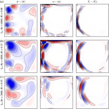
Snapshots of deviations from their time averages for streamfunction, vorticity and horizontal temperature gradient, for the limit cycles at parameter points
 $(\mathit{Re},\mathit{Ri})$
as indicated. Supplementary movie 1, available at https://doi.org/10.1017/jfm.2018.656, shows animations of
 $\unicode[STIX]{x1D713}-\langle \unicode[STIX]{x1D713}\rangle$
for each limit cycle over one period.
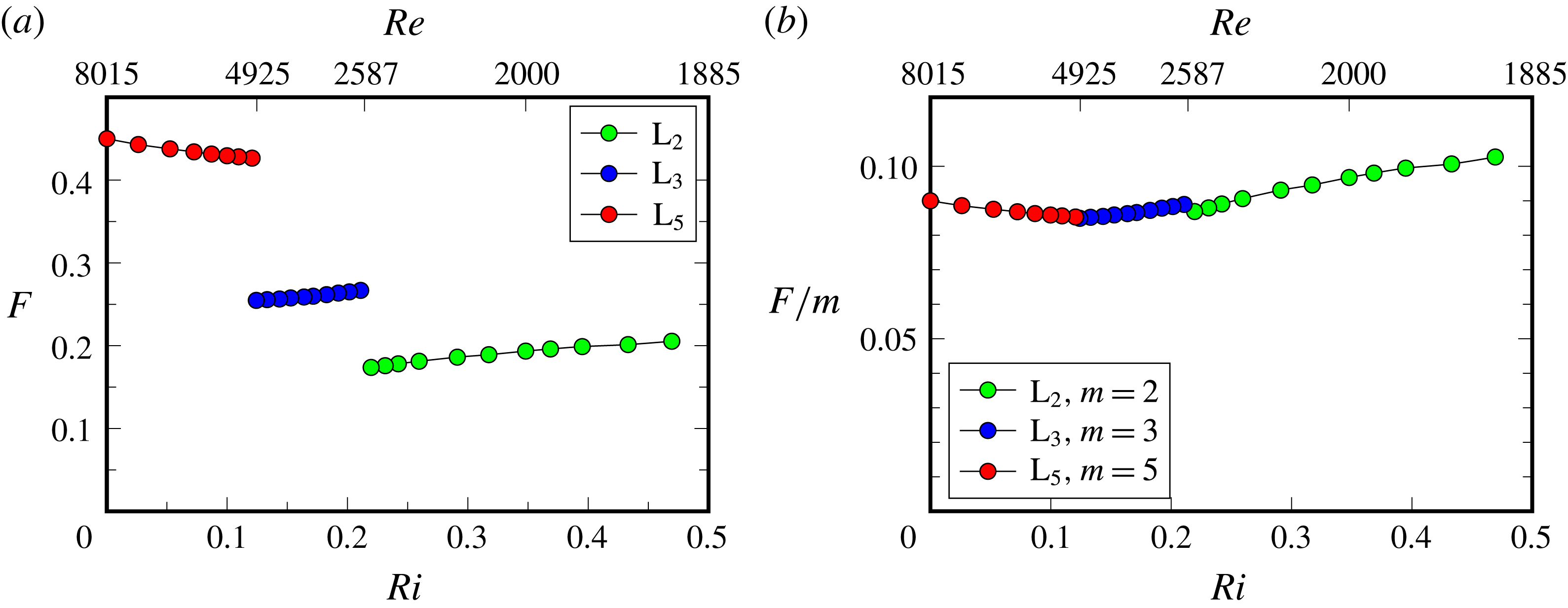
(a) Scaled frequencies
 $F$
of the limit cycles L
 $_{2}$
, L
 $_{3}$
and L
 $_{5}$
at
 $\mathit{Ri}$
and
 $\mathit{Re}$
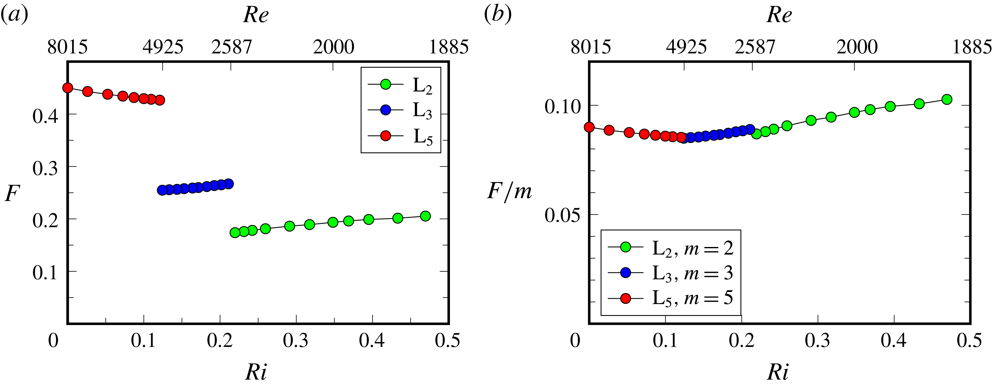
slightly beyond the supercritical Hopf bifurcations shown in figure 2, and (b) the corresponding scaled frequencies
 $F/m$
.
For
 $\mathit{Ri}<0.5$
, the steady state S loses stability as
 $\mathit{Re}$
is increased beyond a critical value via supercritical Hopf bifurcations, resulting in time periodic flows. At
 $\mathit{Ri}=0$
, oscillations appear at the critical
 $\mathit{Re}\approx 8016$
(using a
 $128\times 128$
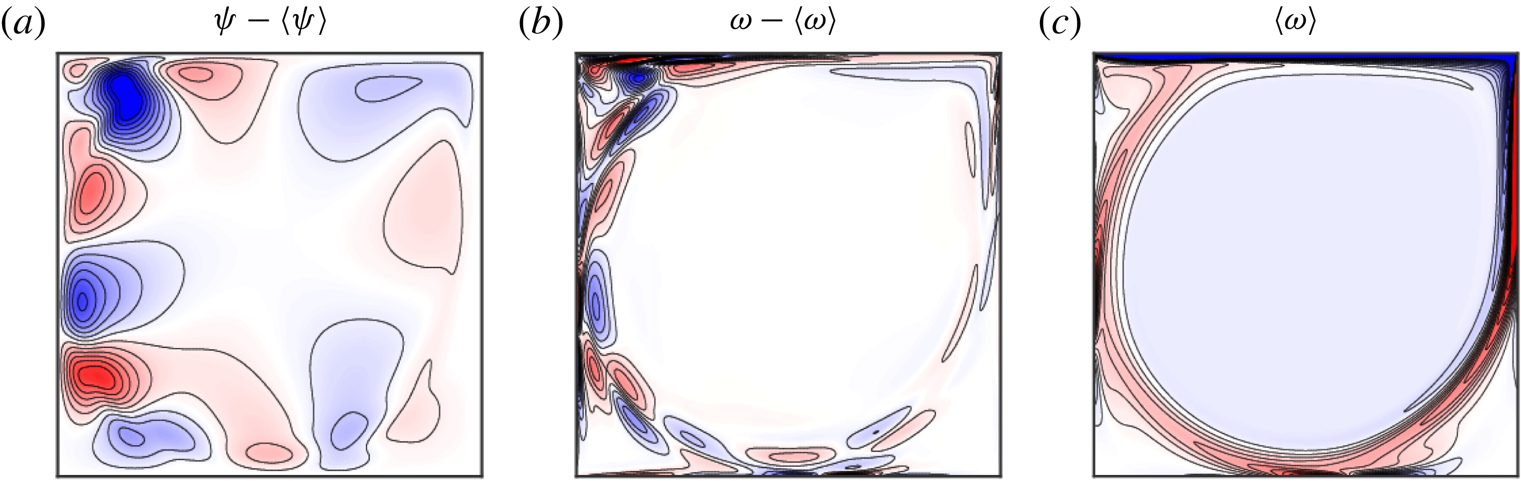
Chebyshev grid), which compares well with values in Brezillon, Girault & Cadou (Reference Brezillon, Girault and Cadou2010, table 3) obtained using various different numerical approaches and top-corner velocity regularisations. Figure 5 shows snapshots of the deviations from the time averages of the streamfunction and the vorticity,
 $\unicode[STIX]{x1D713}-\langle \unicode[STIX]{x1D713}\rangle$
and
 $\unicode[STIX]{x1D714}-\langle \unicode[STIX]{x1D714}\rangle$
, as well as the time-averaged vorticity,
 $\langle \unicode[STIX]{x1D714}\rangle$
. The deviation from the mean streamfunction is comprised of
 $5$
negative cells interlaced with
 $5$
positive cells which propagate around the periphery of the roller in the clockwise direction. This
 $m=5$
cycle is denoted L
 $_{5}$
. The structure of L
 $_{5}$
is similar to that of the real and imaginary parts of the critical Hopf eigenmode reported in Brezillon et al. (Reference Brezillon, Girault and Cadou2010, figure 8), Poliashenko & Aidun (Reference Poliashenko and Aidun1995, figure 2), Fortin et al. (Reference Fortin, Jardak, Gervais and Pierre1997, figure 5) and Auteri, Parolini & Quartapelle (Reference Auteri, Parolini and Quartapelle2002, figure 14). The scaled angular frequency of L
 $_{5}$
is
 $F\approx 0.45$
, which matches the frequency values reported in Brezillon et al. (Reference Brezillon, Girault and Cadou2010, table 3). This frequency corresponds to the rate at which a cell replaces the next cell of the same sign. Consequently,
 $F/m\approx 0.09$
is the fundamental frequency associated with a complete rotation of a given cell around the roller.
As
 $\mathit{Ri}$
increases from
 $0$
, the critical
 $\mathit{Re}$
decreases. The curve in
 $(\mathit{Ri},\mathit{Re})$
-space along which S loses stability is made up of three distinct Hopf bifurcation curves H
 $_{m}$
, with
 $m=5$
, 3 and 2 associated with three different limit cycles L
 $_{m}$
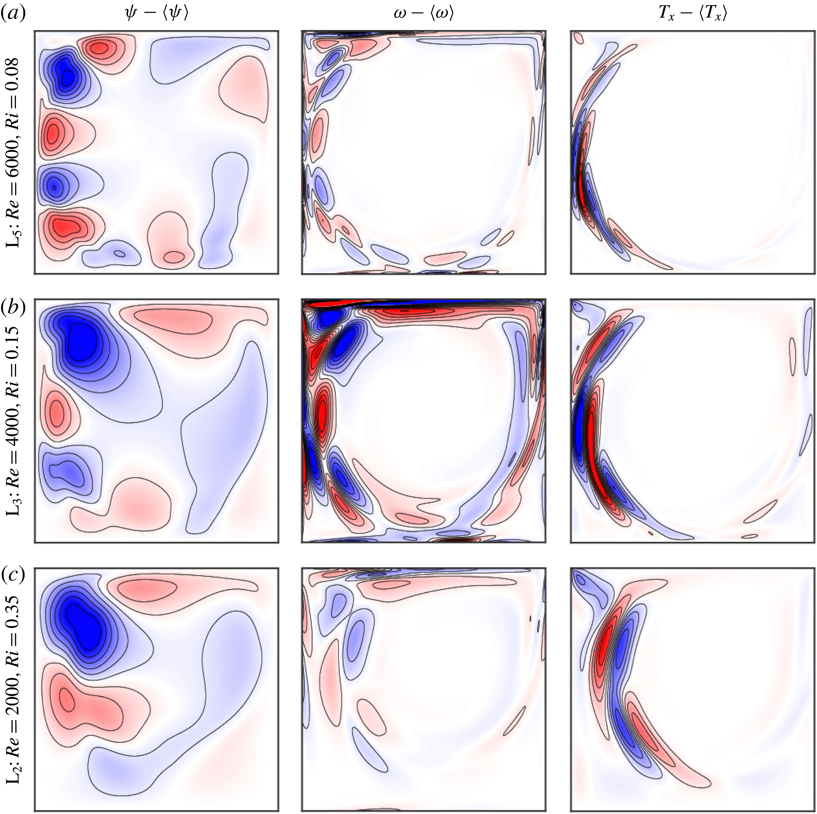
. Figure 6 illustrates the streamfunction, vorticity and horizontal temperature gradient deviations from their time averages for L
 $_{5}$
, L
 $_{3}$
and L
 $_{2}$
, computed at
 $\mathit{Re}$
slightly above critical for
 $\mathit{Ri}=0.08$
, 0.15 and 0.35. Movies of
 $\unicode[STIX]{x1D713}-\langle \unicode[STIX]{x1D713}\rangle$
for the three limit cycles over one period are available in supplementary movie 1. The streamfunction deviations of L
 $_{m}$
show
 $m$
pairs of interlacing negative and positive cells. While it may be difficult to count the number of cell pairs from a single snapshot due to their elongation at the windward vertical wall, the animations in movie 1 make this task much easier as the cells propagate around the periphery of the roller. The structure of L
 $_{5}$
at
 $\mathit{Ri}=0.08$
is essentially the same as that of L
 $_{5}$
at
 $\mathit{Ri}=0$
in figure 5. The cells thicken as their number
 $2m$
becomes smaller in different regions of
 $(\mathit{Ri},\mathit{Re})$
-space. The frequencies of the limit cycles at the bifurcation are shown in figure 7. For smaller
 $m$
, the larger cell size of L
 $_{m}$
leads to a lower scaled angular frequency
 $F$
, but the rotation number
 $F/m$
exhibits little variation along the three Hopf bifurcation curves, and is almost continuous across modal transitions.
The Hopf curves intersect each other at double-Hopf bifurcation points. There are two of these for
 $\mathit{Ri}<0.5$
: dH
 $_{23}$
at
 $(\mathit{Ri},\mathit{Re})\approx (0.214,2587)$
and dH
 $_{35}$
at
 $(\mathit{Ri},\mathit{Re})\approx (0.1245,4925)$
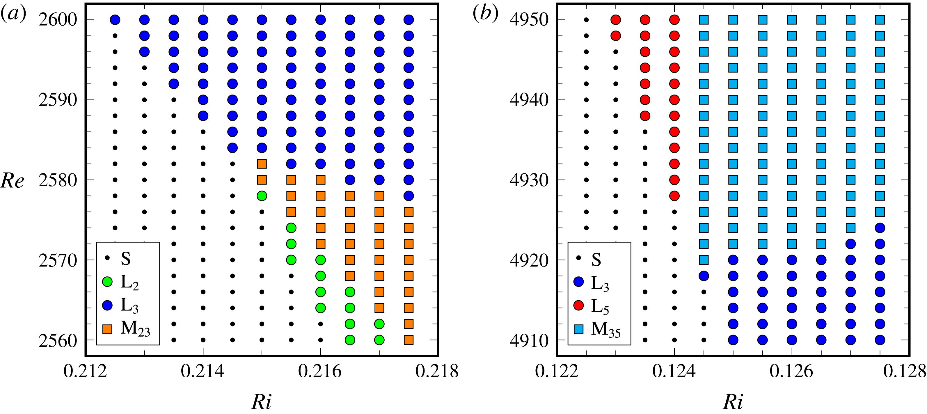
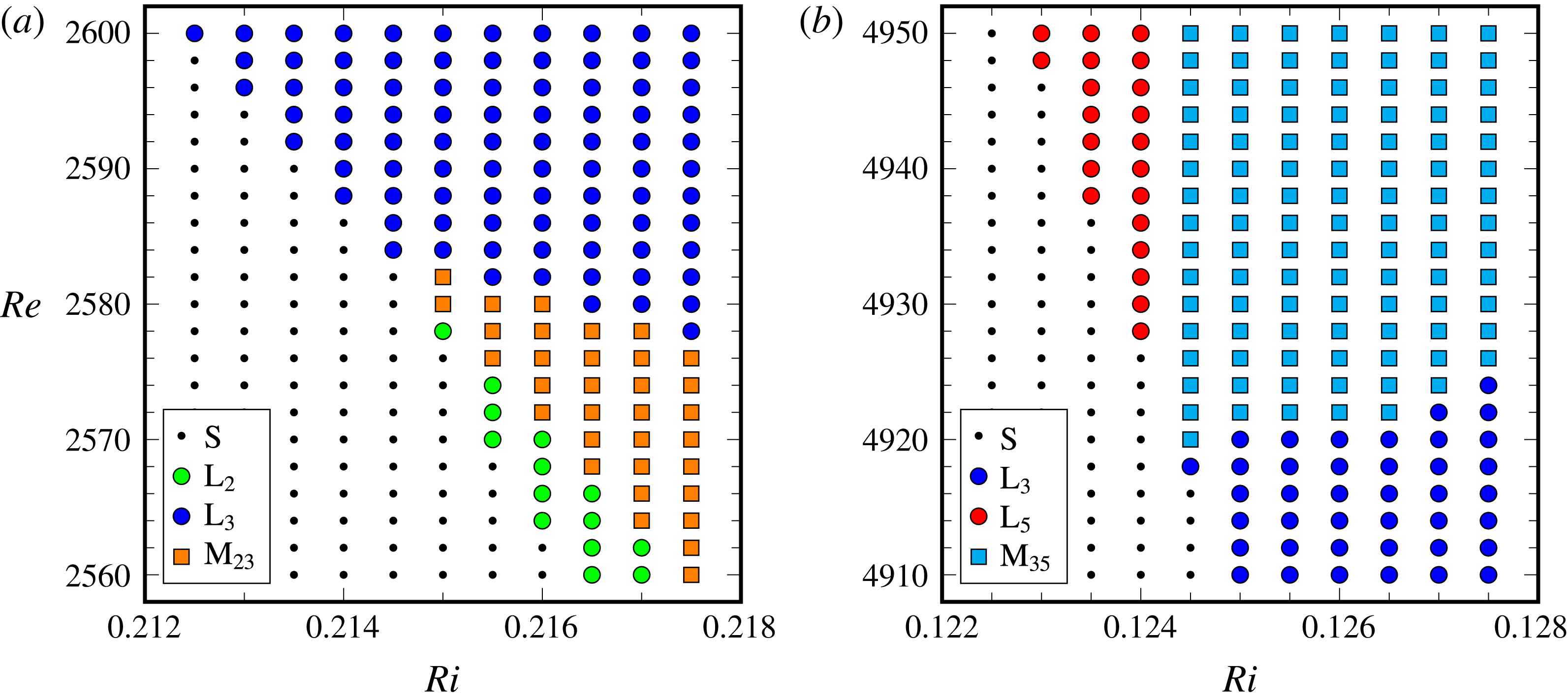
. Typically, in the neighbourhood of a double-Hopf point, a quasi-periodic mixed mode of the two limit cycles involved also exists, and in some cases the mixed modes is stable (Kuznetsov Reference Kuznetsov2004). This is the case here for the two double-Hopf bifurcations, as shown in figure 8. The mixed modes M
 $_{23}$
and M
 $_{35}$
are essentially superpositions of the limit cycles L
 $_{2}$
and L
 $_{3}$
, and L
 $_{3}$
and L
 $_{5}$
, respectively, and are stable in parameter regimes emerging from the double-Hopf points. In the regions where the mixed modes are stable, the limit cycles are not. The boundaries separating the parameter regions where the mixed mode is stable and the two regions where the limit cycles are stable are curves of Neimark–Sacker bifurcations. The slopes of these curves and of the Hopf bifurcations curves very close to the double-Hopf point provide estimates of the normal-form coefficients of the two double-Hopf bifurcations. From these, one can determine the nonlinear behaviour of the flow states. In the classification of Kuznetsov (Reference Kuznetsov2004, § 8.6), dH
 $_{35}$
is simple type II, while the approximate alignment of the Hopf curve H
 $_{3}$
with a Neimark–Sacker curve prevents the distinction between simple type II or simple type III for dH
 $_{23}$
(Kuznetsov Reference Kuznetsov2004, figure 8.25). Nevertheless, both simple type II and simple type III double-Hopf bifurcations are cases with the mixed mode being stable.
Stable states observed via continuation of the steady state by increasing
 $\mathit{Ri}$
at fixed
 $\mathit{Re}$
in the indicated parameter ranges. The presence of two stable limit cycle solutions and a stable (quasi-periodic) mixed state indicate the presence of two supercritical Hopf branches intersecting at double-Hopf points corresponding to (a) dH
 $_{23}$
and (b) dH
 $_{35}$
.
4.3 Instability of S for
$\mathit{Ri}>0.5$
: subcritical Hopf bifurcations

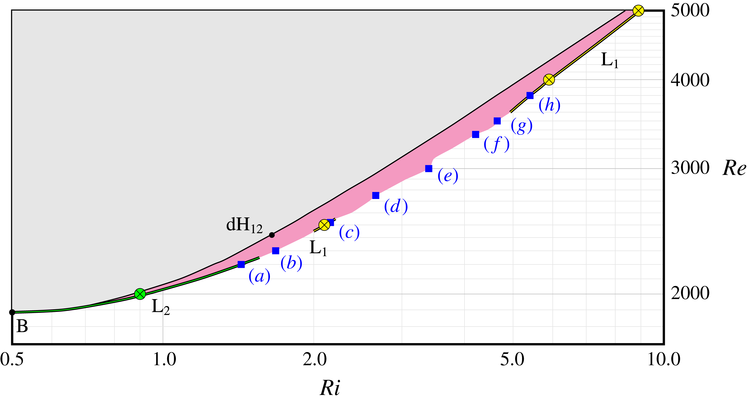
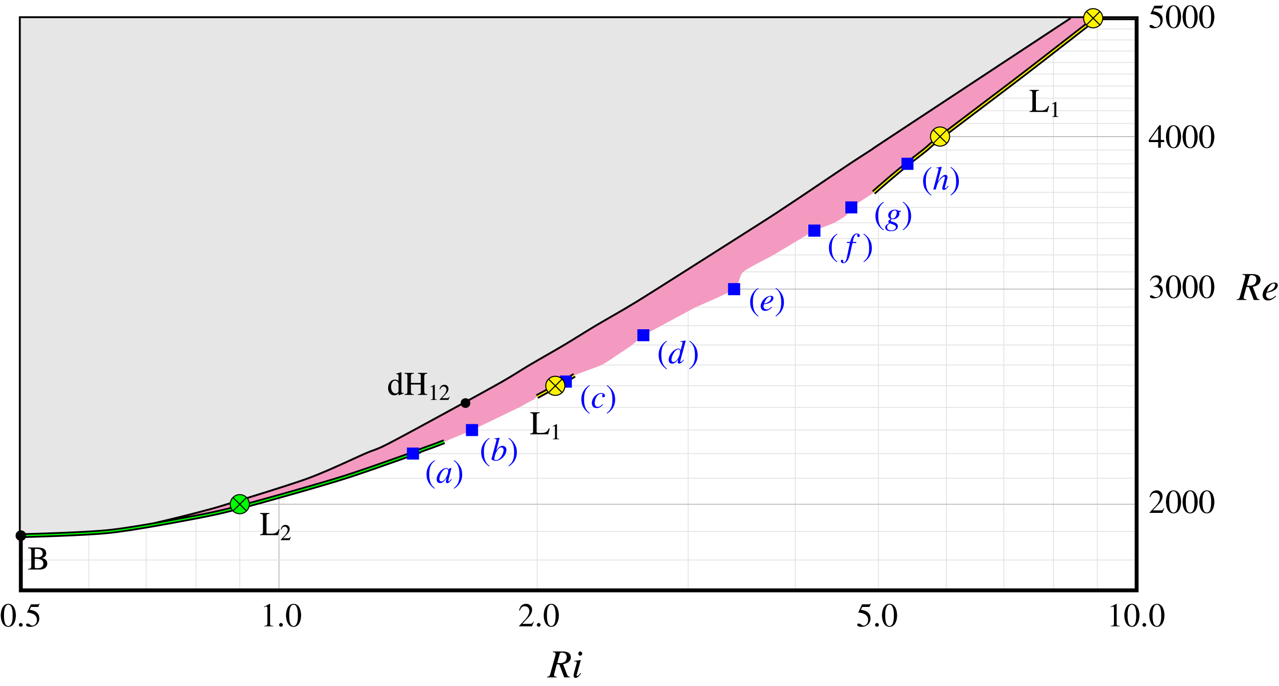
Close up from figure 2 of the hysteresis region (shaded magenta) starting from the Bautin point B, between the subcritical Hopf curve where the steady state loses stability and the cyclic-fold curve. The
 $\otimes$
symbols indicate the locations in
 $(\mathit{Re},\mathit{Ri})$
space where examples of limit cycles L
 $_{2}$
and L
 $_{1}$
are shown in figure 10. Time series of
 $E$
and phase portraits of sample states at the edge of the hysteresis region indicated by the blue squares labelled (a–h) are shown in figure 11.
For
 $\mathit{Ri}\gtrsim 0.5$
, the steady state S loses stability as
 $\mathit{Re}$
increases via a subcritical Hopf bifurcation. The Bautin point B at which the Hopf bifurcation H
 $_{2}$
switches from being supercritical to subcritical is at
 $(\mathit{Ri},\mathit{Re})\approx (0.5,1885)$
. At this point a cyclic-fold (saddle-node bifurcation of limit cycles) bifurcation curve also emerges, along which the unstable limit cycle L
 $_{2}$
created at the subcritical H
 $_{2}$
bifurcation (the lower branch cycle) becomes stable (upper branch cycle) as it is folded back in parameter space (Kuznetsov Reference Kuznetsov2004). Both S and upper branch L
 $_{2}$
co-exist and are stable, and lower branch L
 $_{2}$
is unstable in the hysteresis region between the subcritical Hopf and cyclic-fold curves, the region shaded magenta in figure 2; also see the close-up version in figure 9 where the cyclic-fold curve of L
 $_{2}$
is drawn as a thick green curve on the high-
 $\mathit{Ri}$
/low-
 $\mathit{Re}$
edge of the hysteresis region. This cyclic-fold curve which starts at the Bautin point B ends at
 $(\mathit{Ri},\mathit{Re})\approx (1.56,2250)$
. Beyond this point, the upper branch state is a quasi-periodic state all the way to the edge of the hysteresis region. Then, at the edge of the hysteresis region at
 $(\mathit{Ri},\mathit{Re})\approx (2,2450)$
, the edge is once again a cyclic-fold bifurcation, but now involving a limit cycle L
 $_{1}$
. The extent of this cyclic-fold curve is drawn as a thick yellow line in figure 9. The frequencies of L
 $_{1}$
and L
 $_{2}$
on the upper branches of the respective cyclic-fold bifurcations are very close to a 1 : 2 frequency ratio, and the spectral signature of the quasi-periodic state has all linear combinations of these two frequencies. This behaviour is indicative of an underlying double-Hopf bifurcation dH
 $_{12}$
, where both Hopf bifurcations from the steady state S are subcritical. This codimension-two point is estimated to be at
 $(\mathit{Ri},\mathit{Re})\approx (1.65,2420)$
, indicated in the phase diagram figure 2, as well as in figure 9. This type of double-Hopf bifurcation is strongly resonant and in its neighbourhood, homoclinic and heteroclinic dynamics and transverse intersections of stable and unstable manifolds are to be expected, leading to slow–fast dynamics and chaotic behaviour. This complex dynamics is associated with the phase of the limit cycles not decoupling from their amplitude, opening up the possibility for the phases of the two limit cycles to lock and unlock via heteroclinic bifurcations (Knobloch & Proctor Reference Knobloch and Proctor1988). The cyclic-fold curve of L
 $_{1}$
is short, extending only to
 $(\mathit{Ri},\mathit{Re})\approx (2.2,2550)$
, beyond which the upper branch states at the edge of the hysteresis region are quasi-periodic or more complex (some are described below). Further along the edge, from
 $(\mathit{Ri},\mathit{Re})\approx (5,3600)$
to at least
 $(\mathit{Ri},\mathit{Re})\approx (9,5000)$
, the edge is once again demarcated by a cyclic-fold curve of L
 $_{1}$
(also drawn as a thick yellow line in figure 9).
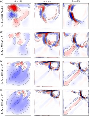
Figure 10 shows snapshots of the streamfunction, vorticity and horizontal temperature gradient deviations from their time averages for the limit cycles L
 $_{1}$
and L
 $_{2}$
near the cyclic-fold bifurcation curves described above, at
 $(\mathit{Ri},\mathit{Re})$
points indicated as
 $\otimes$
in figure 9. For L
 $_{2}$
at
 $(\mathit{Ri},\mathit{Re})=(0.9,2000)$
, the two cells of each sign in the streamfunction deviation (blue and red) are easily recognisable, and to a lesser extent in the vorticity and horizontal temperature gradient deviations. At this relatively small
 $\mathit{Ri}$
, the lid-driven roller occupies most of the cavity. At larger
 $\mathit{Re}$
and
 $\mathit{Ri}$
, L
 $_{1}$
with a large single pair of cells in the streamfunction deviation is the state undergoing the cyclic-fold bifurcation. At these larger
 $\mathit{Ri}$
, the roller is more confined to the downstream top corner region and the lower part of the cavity is nearly linearly stratified. The ratio of the L
 $_{1}$
frequency and the local buoyancy frequency in the lower part of the cavity is such that internal wave beams are emitted from the oscillatory roller into the stratified region at an angle of approximately
 $45^{\circ }$
such that they reflect back from lower left corner of the cavity. This retracing of the beam leads to enhanced phase coherence. Supplementary movie 2 shows
 $T_{x}-\langle T_{x}\rangle$
for the four cases in figure 10, each animated over one period. In the movie, it is evident that, even for the L
 $_{2}$
case with the relatively small
 $\mathit{Ri}$
, there is a hint of a wave beam also retracing off the lower left corner. The energy of the wave beams does not exceed a few per cent of the total energy.
Snapshots of deviations from their time averages for streamfunction, vorticity and horizontal temperature gradient, for the limit cycles at parameter points
 $(\mathit{Re},\mathit{Ri})$
as indicated. Supplementary movie 2 shows animations of
 $T_{x}-\langle T_{x}\rangle$
for over one period.

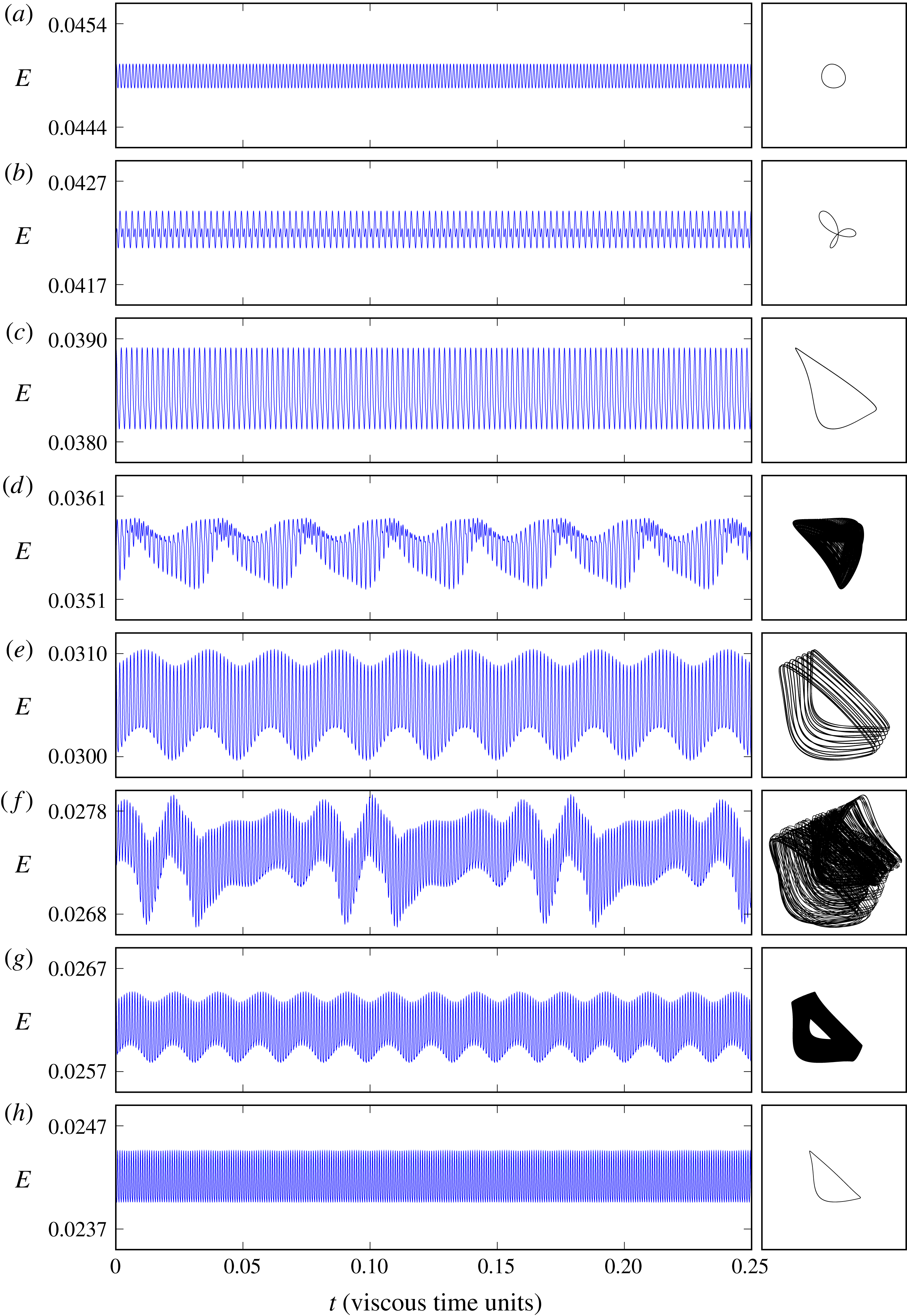
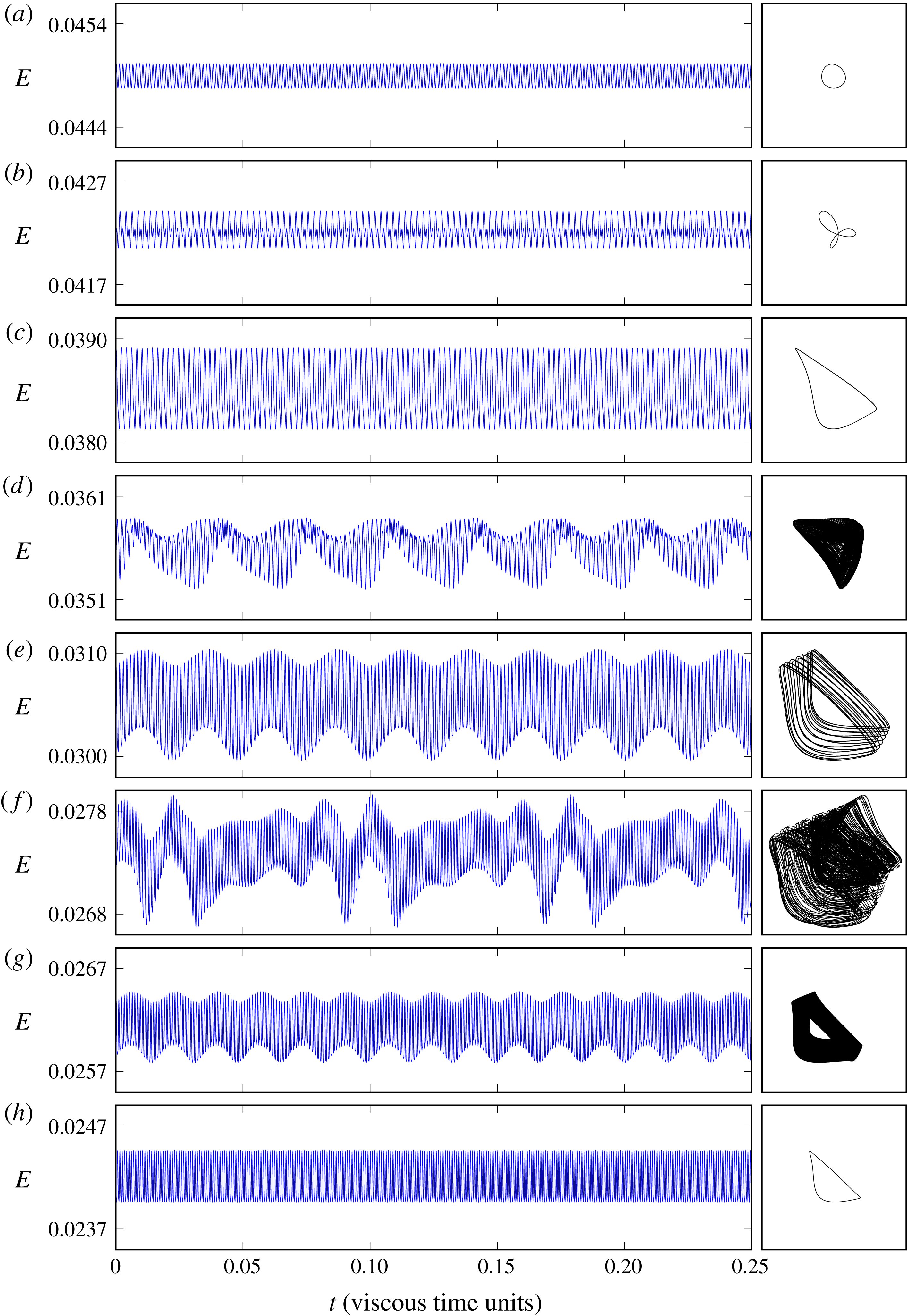
Time series of the
 $\mathit{E}$
responses over a window of
 $0.25$
viscous units, at the
 $(\mathit{Ri},\mathit{Re})$
values indicated in figure 9 by the locations of the labels (a–h), together with the corresponding phase portraits using
 $(\mathit{E}(t-\unicode[STIX]{x1D70F}),\mathit{E}(t))$
with delay
 $\unicode[STIX]{x1D70F}=1/(0.3\mathit{Re}\sqrt{1+\mathit{ Ri}})$
.
Between
 $(\mathit{Ri},\mathit{Re})\approx (2.2,2550)$
and
 $(\mathit{Ri},\mathit{Re})\approx (5,3600)$
, the last state observed on the upper branch of the hysteresis region before falling back to the steady state as
 $\mathit{Ri}$
is increased is a quasi-periodic (QP) state with strong L
 $_{1}$
content. A pure L
 $_{1}$
is also observed slightly below
 $(\mathit{Ri},\mathit{Re})\approx (5,3600)$
, suggesting a subcritical bifurcation along the fold between the QP and L
 $_{1}$
states.
Figure 11 illustrates specific responses obtained along the upper branch, at the last stable time-dependent state obtained when increasing
 $\mathit{Ri}$
, labelled (a–h) in figure 9. The plots show the time series
 $\mathit{E}(t)$
over 0.25 viscous time units as well as phase portraits obtained by plotting
 $\mathit{E}(t)$
against a delayed
 $\mathit{E}(t-\unicode[STIX]{x1D70F})$
. The delay
 $\unicode[STIX]{x1D70F}$
was selected such that the associated frequency
 $F=1/(\unicode[STIX]{x1D70F}\mathit{Re}\sqrt{1+\mathit{ Ri}}\,)=0.3$
is larger, but not excessively so, than the scaled frequency
 $F\approx 0.2$
of L
 $_{2}$
. The responses (a) and (c) correspond to limit cycles L
 $_{2}$
and L
 $_{1}$
respectively. Limit cycle L
 $_{1}$
is also the response in
 $(h)$
, and its presence can be recognised in the quasi-periodic responses (e,f,g), with the low beat frequency and the frequency of L
 $_{1}$
locked in a 1 : 18 ratio in case (e). Case (b) illustrates a locked mixed mode of L
 $_{1}$
and L
 $_{2}$
in a regime close to the double-Hopf point dH
 $_{12}$
. This mixed mode seems to arise from a flip bifurcation of L
 $_{2}$
(Floquet multiplier crossing the unit circle at
 $-1$
) at a lower
 $\mathit{Ri}$
(or
 $\mathit{Re}$
). Response (d) exhibits near heteroclinic behaviour between limit cycles L
 $_{1}$
and L
 $_{2}$
, with about equal power at both frequencies, again likely associated with the strongly resonant double-Hopf bifurcation H
 $_{12}$
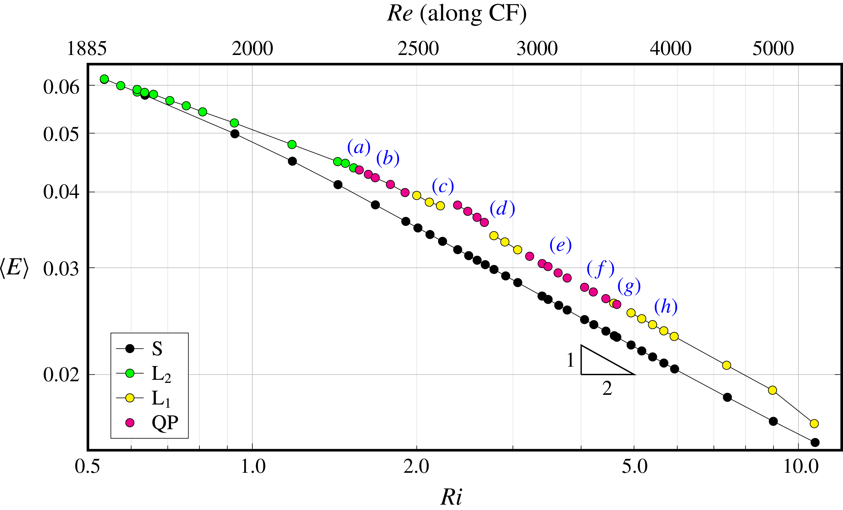
. A plot of the (long) time average of the scaled kinetic energy
 $\langle \mathit{E}\rangle$
along the upper branch of the fold in figure 12 shows that the mixed mode in case (d) has slightly higher kinetic energy than its L
 $_{1}$
neighbours.
The scaling
 $\mathit{Re}\sim \sqrt{\mathit{Ri}}$
holds along the subcritical Hopf curve (black line in figure 2). This scaling can be justified near the onset of instability of the base steady state S at large
 $\mathit{Ri}$
and
 $\mathit{Re}$
by assuming a linear stratification, so that
 $$\begin{eqnarray}\boldsymbol{u}=(u(z,t),w(x,t)),\quad p=p(x,t),\quad T_{x}=T_{zz}=0.\end{eqnarray}$$
In this case, the system (2.1) simplifies to
 $$\begin{eqnarray}u_{t}+wu_{z}=-p_{x}+u_{zz},\quad w_{t}+uw_{x}=w_{xx}+\mathit{Gr}\,T,\quad T_{t}+wT_{z}=T_{xx}/\mathit{Pr}.\end{eqnarray}$$
In the steady case, this further reduces to
 $$\begin{eqnarray}w_{xxxx}=uw_{xxx}-\mathit{Gr}\,T_{xx}=uw_{xxx}-r^{4}w,\end{eqnarray}$$
where
 $r^{4}=T_{z}\mathit{Gr}\mathit{Pr}$
. The existence of a similarity solution
 $w=w(rx)$
leads to the condition
 $u\sim r$
, i.e.
 $\mathit{Re}\sim r\sim \sqrt[4]{\mathit{Gr}}$
using the entrainment condition
 $u=-\mathit{Re}$
at the top of the stratified region. Similar arguments for a related problem are made in Hanratty, Rosen & Kabel (Reference Hanratty, Rosen and Kabel1958), and in Blanchette et al. (Reference Blanchette, Peacock and Cousin2008) who also present supporting physical experiments.
Scaled kinetic energy
 $\mathit{E}$
of steady states and mean time scaled kinetic energy
 $\langle \mathit{E}\rangle$
of unsteady states along the cyclic-fold upper branch as functions of
 $\mathit{Ri}$
. The points labelled (a–h) correspond to the same labelled points in figure 9.

In the time-dependent case, balancing the terms in (4.2) and assuming the solution to be periodic with angular frequency
 $\unicode[STIX]{x1D714}$
yields
 $$\begin{eqnarray}\unicode[STIX]{x1D714}^{2}w\sim w_{tt}\sim \mathit{Gr}~T_{t}\sim \mathit{Gr}~T_{z}w,\end{eqnarray}$$
i.e.
 $\unicode[STIX]{x1D714}\sim \sqrt{\mathit{Gr }~T_{z}}$
. So, for large
 $\mathit{Ri}$
,
 $$\begin{eqnarray}F\sim \frac{\unicode[STIX]{x1D714}/2\unicode[STIX]{x03C0}}{\mathit{Re}\sqrt{\mathit{Ri}}}=\frac{\unicode[STIX]{x1D714}/2\unicode[STIX]{x03C0}}{\sqrt{\mathit{Gr}}}\sim \frac{\sqrt{T_{z}}}{2\unicode[STIX]{x03C0}}\sim \frac{1}{2\unicode[STIX]{x03C0}}\approx 0.159,\end{eqnarray}$$
approaches a constant, further justifying the choice of the frequency scaling (3.4).
The data in figure 12 also suggest the scaling
 $$\begin{eqnarray}\langle \mathit{E}\rangle \sim 1/\sqrt{\mathit{Ri}}\sim 1/\mathit{Re}\sim 1/\sqrt[4]{\mathit{Gr}},\end{eqnarray}$$
along the fold curves. There, the peak frequency
 $f$
of the response scales like
 $$\begin{eqnarray}f=F\,\mathit{Re}\sqrt{1+\mathit{ Ri}}\sim \mathit{Re}\sqrt{\mathit{Ri}}\sim \mathit{Ri},\end{eqnarray}$$
resulting in
 $\langle \mathit{E}\rangle \sim 1/\sqrt{f}$
.
The scaled frequency of L
 $_{1}$
along its fold above
 $(\mathit{Ri},\mathit{Re})\approx (5,3600)$
was observed to marginally increase from
 $F\approx 0.115$
to
 $F\approx 0.118$
at
 $(\mathit{Ri},\mathit{Re})\approx (9,5000)$
. However, at
 $(\mathit{Ri},\mathit{Re})\approx (10.7,5500)$
(corresponding to the rightmost upper data point in figure 12) the scaled frequency
 $F$
of L
 $_{1}$
at its fold was found to be significantly higher, namely
 $F\approx 0.135$
, which is much closer to the value predicted by (4.5).
Variation of the power spectrum density (PSD) of
 $\mathit{E}$
with
 $\mathit{Ri}$
, in terms of scaled frequency
 $F$
, for
 $\mathit{Re}$
as indicated. Black corresponds to peak energy at the given
 $\mathit{Re}$
, and white is 50 dB or more below the peak.
4.4 Dynamics above the neutral curve
The flow response for selected
 $\mathit{Re}$
values was computed for
 $\mathit{Ri}\in [10^{-1},10^{1}]$
over at least four viscous times, and up to 15 viscous times for cases with low-frequency content. Responses associated with a coarse grid of logarithmically spaced
 $\mathit{Ri}$
values were first obtained using zero velocity and a linear temperature profile as the initial condition. The responses for intermediate
 $\mathit{Ri}$
were then obtained via continuation using these solutions as initial conditions. No systematic effort was made to identify multiple stable solutions, which do exist in certain parameter regimes (resulting in hysteresis), except in the subcritical band in the upper
 $\mathit{Ri}$
range (the region shaded magenta in figures 2 and 13), where both the base state
 $S$
and a time-dependent solution are stable and co-exist. In this region, a detailed investigation to find the edges of the hysteresis band was executed using a variety of different initial conditions.
Peak power and corresponding
 $\mathit{Ri}$
of
 $\mathit{E}$
spectral data at
 $\mathit{Re}$
as indicated.

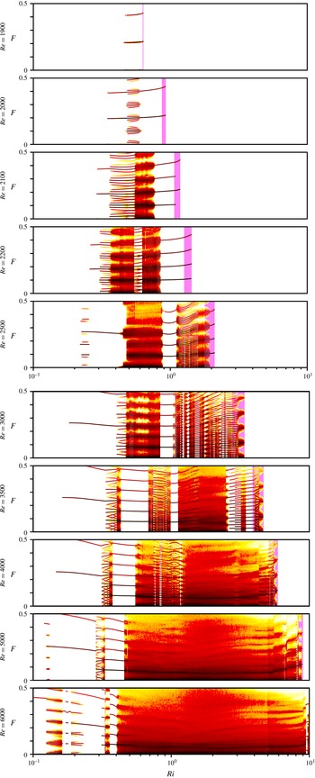
An overview of the unsteady flow response over the extensive
 $(\mathit{Ri},\mathit{Re})$
parameter regime considered is presented in figure 13, which provides, for each
 $\mathit{Re}$
considered, the variation with
 $\mathit{Ri}$
of the power spectral density (PSD) of the
 $\mathit{E}$
time series. To obtain the individual PSDs, the
 $\mathit{E}$
time series were first trimmed to remove transients, de-trended and Blackman filtered. The resulting PSDs were collated and normalised to peak power over all
 $\mathit{Ri}$
values for each given
 $\mathit{Re}$
. Table 1 contains the values of the normalising peak power of the PSD for each
 $\mathit{Re}$
value, as well as the
 $\mathit{Ri}$
value at the peaks. Since
 $\mathit{E}$
already includes a scaling
 $\mathit{Re}^{2}$
, these peak values merely represent the pre-factor for this scaling, and allow comparisons across different
 $\mathit{Re}$
. Note that peak power is consistently reached at
 $\mathit{Ri}\approx 0.6$
, i.e. when shear and buoyancy forces are of comparable strength. Figure 13 illustrates the increasing complexity of the responses as
 $\mathit{Re}$
is increased. It shows a ‘view from the top’ of the normalised PSDs as a function of
 $\mathit{Ri}$
obtained for each
 $\mathit{Re}$
as indicated, with a colour scale from white (low energy) to red/black (high energy), corresponding to a power ratio of
 $10^{5}$
(50 dB range). Values below
 $10^{-5}$
of peak power were omitted (set to white).
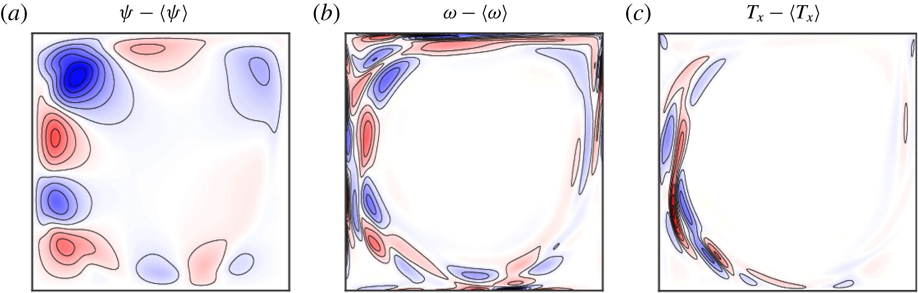
Snapshots of the deviations from their mean for streamfunction, vorticity and horizontal temperature gradient for the limit cycle L
 $_{4}$
at
 $\mathit{Re}=6000$
and
 $\mathit{Ri}=0.17$
.

As
 $\mathit{Re}$
increases, the
 $\mathit{Ri}$
band over which an unsteady response is obtained widens. At the lower
 $\mathit{Ri}$
end of this range, the spectra is that of a pure limit cycle (single frequency plus harmonics), identified as L
 $_{2}$
for
 $\mathit{Re}\approx 1900$
–
 $2500$
, L
 $_{3}$
for
 $\mathit{Re}\approx 3000$
–
 $5000$
and L
 $_{5}$
for
 $\mathit{Re}\approx 5000$
and
 $6000$
. At both
 $\mathit{Re}=2500$
and
 $\mathit{Re}=5000$
, the respective limit cycles L
 $_{2}$
and L
 $_{5}$
quickly transform into quasi-periodic states, and then into limit cycle L
 $_{3}$
as
 $\mathit{Ri}$
increases across the Neimark–Sacker bifurcation curves emanating from the nearby double-Hopf points, dH
 $_{23}$
and dH
 $_{35}$
, described earlier. A pure limit cycle L
 $_{4}$
(figure 14), was also observed at
 $\mathit{Re}=6000$
in a small range with
 $\mathit{Ri}\approx 0.17$
, close to the supercritical Hopf bifurcation curve H
 $_{5}$
, suggesting the presence of another Hopf bifurcation H
 $_{4}$
. In the parameter regime considered, this Hopf bifurcation is not a primary instability of the basic state S. The scaled frequency of L
 $_{4}$
is
 $F\approx 0.325$
, giving a rotation number
 $F/4\approx 0.081$
, which is comparable to those of the other limit cycles shown in figure 7(b).
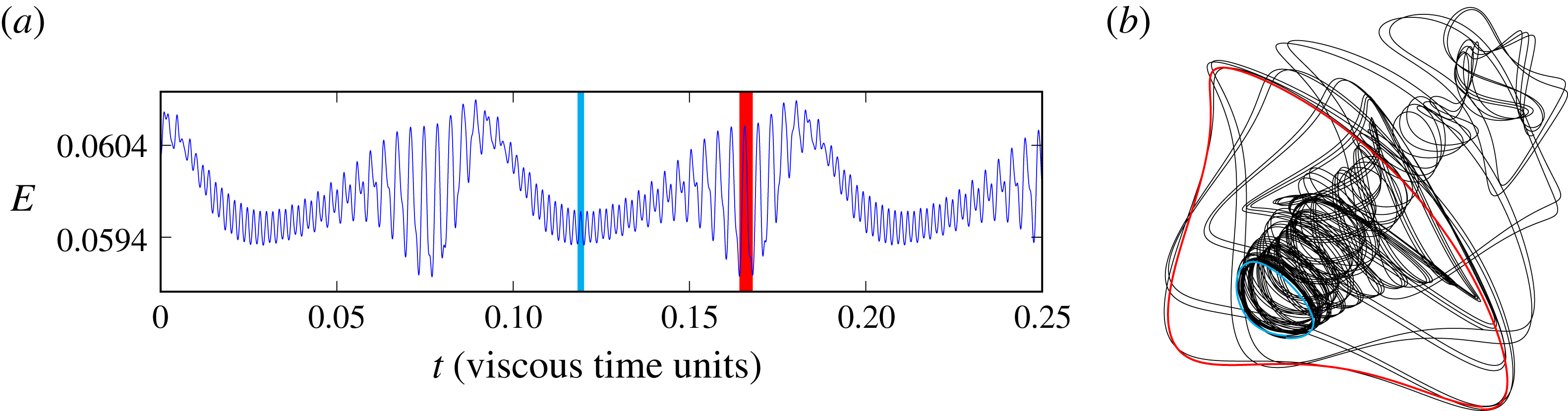
An example of global heteroclinic dynamics at
 $(\mathit{Ri},\mathit{Re})=(0.6902,2100)$
: (a) time series of the response
 $\mathit{E}$
over a window of
 $0.25$
viscous units and (b) corresponding phase portrait
 $(\mathit{E}(t-\unicode[STIX]{x1D70F}),\mathit{E}(t))$
with delay
 $\unicode[STIX]{x1D70F}=1/(0.3\mathit{Re}\sqrt{1+\mathit{ Ri}})$
.

With increasing
 $\mathit{Ri}$
, the spectra of the computed responses become more complex showing characteristics typical of quasi-periodic flows with incommensurate frequencies. There are intervals in
 $\mathit{Ri}$
where the spectra are periodic, due to the frequencies locking into rational ratios. These lockings are more prevalent at lower
 $\mathit{Re}$
values. The locked regions (Arnol’d tongues) emerge from points along the Neimark–Sacker curves, which have their origin at the various double-Hopf points, and extend and interact far from the immediate vicinity of the double-Hopf points, leading to a panoply of more complex dynamical states featuring low-frequency spectral peaks associated with global homoclinic or heteroclinic behaviour (Boyland Reference Boyland1986).
An example of heteroclinic behaviour is presented in figure 15, which shows the
 $\mathit{E}$
response at
 $\mathit{Re}=2100$
and
 $\mathit{Ri}=0.6902$
. The time series (figure 15
a) consists of a fast low-amplitude oscillation followed by a slower large-amplitude oscillation. This repeats periodically with a period of approximately
 $0.1$
viscous time units. The short segments in the time series highlighted in blue and red correspond to times when the flow is close to the unstable (saddle) limit cycles L
 $_{2}$
and L
 $_{1}$
. The nature of this near-heteroclinic cycle between the two saddle limit cycles is further illustrated in the phase portrait in figure 15(b), where the parts of the phase portrait corresponding to the blue and red segments of the time series are also coloured. These parts of the phase portrait have the same shape as the phase portraits of stable L
 $_{2}$
and L
 $_{1}$
limit cycles in figure 11(a,c). The rest of the phase portrait (in black) corresponds to the slow near-heteroclinic drift between the two limit cycles. These periodic drifts take approximately
 $0.05$
viscous times, which is approximately
 $12$
oscillations of L
 $_{1}$
and
 $24$
oscillations of L
 $_{2}$
.
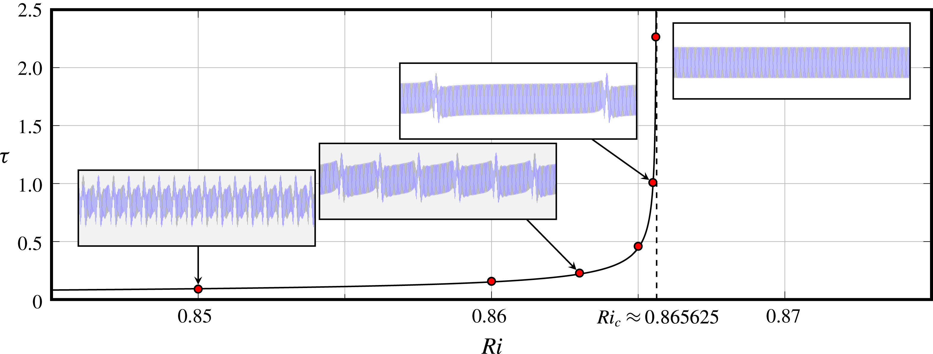
An example of homoclinic dynamics (SNIC on the torus) at
 $\mathit{Re}=2750$
and
 $\mathit{Ri}\approx 0.86$
: the quasi-period
 $\unicode[STIX]{x1D70F}$
(in viscous time units) of a QP state (red bullets) and the black curve is the fit
 $\unicode[STIX]{x1D70F}=0.005+0.011/\sqrt{\mathit{Ri }_{c}-\mathit{ Ri}}$
, where
 $\mathit{Ri}_{c}$
is the critical value of
 $\mathit{Ri}$
at the SNIC bifurcation. The inserts show time series of
 $\mathit{E}\in [0.05,0.06]$
over 1.4 viscous times at the indicated
 $\mathit{Ri}$
. The time series for
 $\mathit{Ri}>\mathit{Ri}_{c}$
show the resulting locked response on the torus.
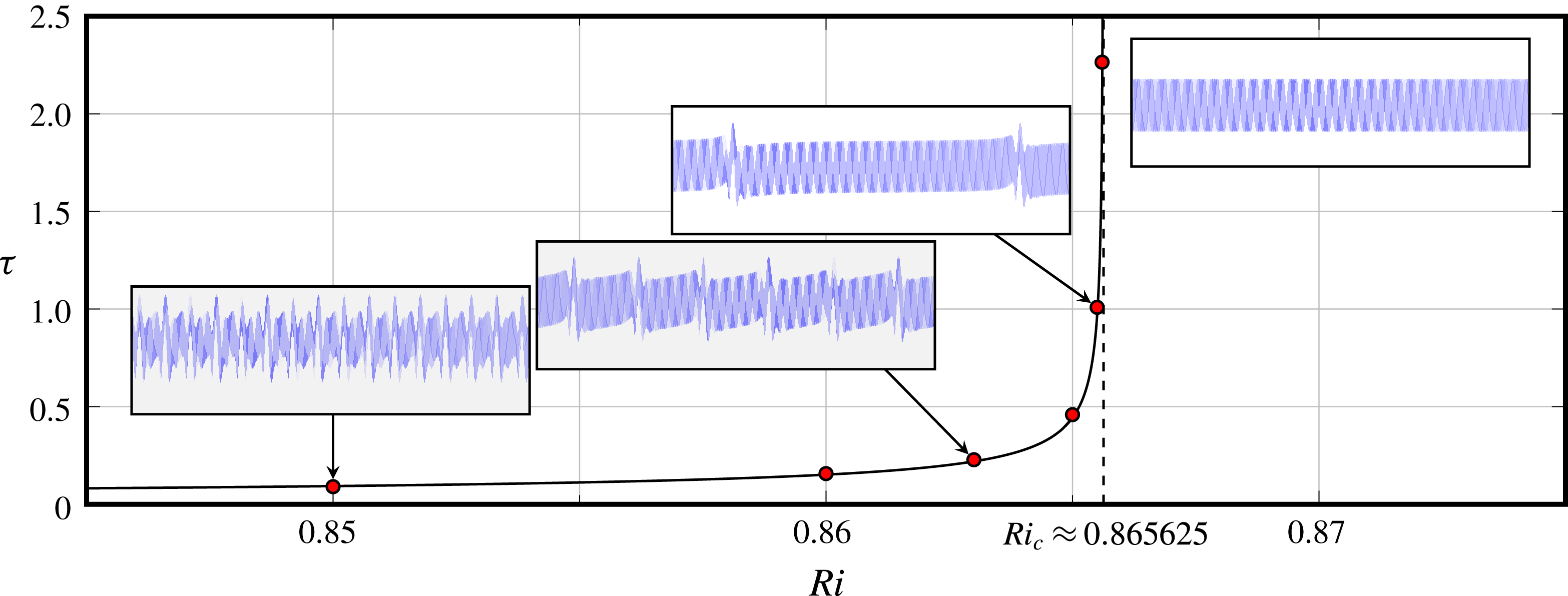
An example of homoclinic behaviour is presented in figure 16, which shows the
 $\mathit{E}$
response at
 $\mathit{Re}=2750$
and selected values of
 $\mathit{Ri}\sim 0.86$
. Below a critical value
 $\mathit{Ri}_{c}\approx 0.865625$
the response is a dyadic quasi-periodic state, with one scaled frequency that hardly varies with
 $\mathit{Ri}$
,
 $F\approx 0.08$
(corresponding to a period of
 $0.033$
viscous times), and a second lower frequency that goes to zero as
 $\mathit{Ri}\rightarrow \mathit{Ri}_{c}$
. The corresponding period goes to infinity as
 $\unicode[STIX]{x1D70F}=0.005+0.011/\sqrt{\mathit{Ri }_{c}-\mathit{ Ri}}$
. The slow–fast behaviour seen in the time series terminates at
 $\mathit{Ri}=\mathit{Ri}_{c}$
with the creation of a pair of limit cycles on the torus, one unstable (saddle) and the other stable (node), at the saddle-node-on-an-invariant-cycle (SNIC) on a torus bifurcation (Lopez & Marques Reference Lopez and Marques2009). For
 $\mathit{Ri}>\mathit{Ri}_{c}$
, only the stable limit cycle on the torus is observed via direct simulations.
Snapshots of the horizontal temperature gradient
 $T_{x}$
of quasi-periodic states at
 $\mathit{Re}=5000$
and
 $\mathit{Ri}$
as indicated; the contours are equispaced in the range
 $|T_{x}|\leqslant 3/\mathit{Ri}$
. Supplementary movie 3 shows animations over
 $0.01$
viscous time.
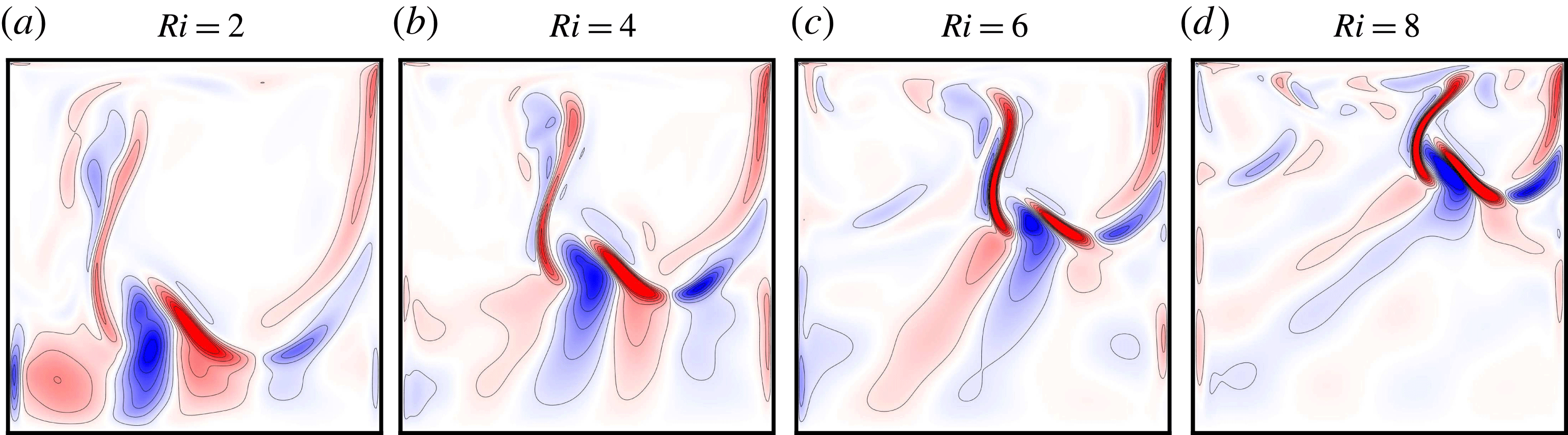
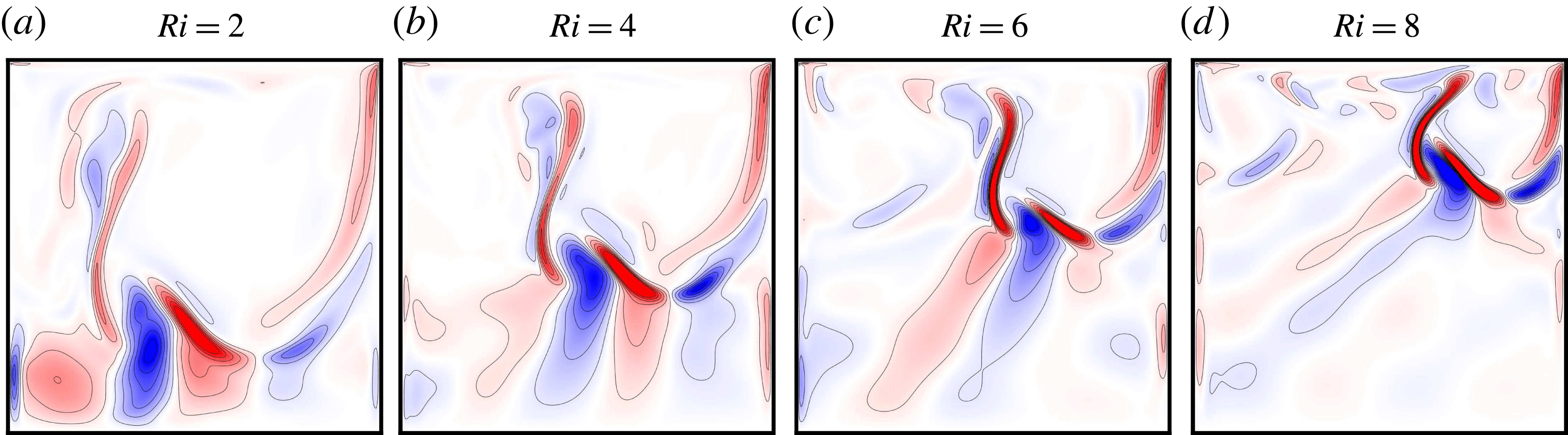
Figure 17 presents snapshots of the horizontal temperature gradient
 $T_{x}$
at
 $\mathit{Re}=5000$
and four selected buoyancy strengths,
 $\mathit{Ri}=2,4,6$
and 8. The four responses are quasi-periodic with a very low-frequency content (see figure 13). The snapshots are shown at a phase when the
 $\mathit{E}$
oscillations are intense. The colour map is scaled by
 $3/\mathit{Ri}$
, so that it is inversely proportional, at fixed
 $\mathit{Re}$
, to the buoyancy intensity measured by the Grashof number
 $\mathit{Gr}$
. With increasing
 $\mathit{Ri}$
, the lid-driven roller is smaller and more confined to the upper downstream corner of the cavity. In all four cases, the relatively strong buoyancy pushes back on the roller quasi-periodically, and the shear forces exerted by the roller scoop up cold fluid from below and drive it up toward the hot lid. With increasing
 $\mathit{Ri}$
, the colder fluid tends to impinge on the top lid and is alternately deflected to the right or to the left. In the latter case, this results in a wave of smaller (boomerang-shaped) cells propagating to the top upstream (left) corner of the cavity. This wave dissipates to some degree in the boundary layers but remains sufficiently strong so as to form a buoyancy barrier identifiable by the (blue, bean-shaped) stationary
 $T_{x}$
cell evident in figures 17(c,d). This dynamics is more clearly evident in the accompanying supplementary movie 3.
Various flip bifurcations have also been detected above the neutral curve. Those occurring at
 $\mathit{Re}=3500$
in the vicinity of
 $\mathit{Ri}=3$
are relatively easy to identify in the PSDs shown in figure 13. For example, a frequency-locked limit cycle arising from a SNIC on the torus at
 $\mathit{Ri}\approx 2.57$
loses stability at
 $\mathit{Ri}\approx 2.63$
via a flip bifurcation, with the resulting period-doubled limit cycle itself losing stability via another flip bifurcation at
 $\mathit{Ri}\approx 2.86$
. The period-quadrupled limit cycle remains stable up to
 $\mathit{Ri}\approx 3.2$
. Beyond
 $\mathit{Ri}=3.2$
, the flow is aperiodic, and then frequency locks again at
 $\mathit{Ri}\approx 3.47$
.
5 Conclusion
The impact of a stable temperature stratification on the flow of a fluid of Prandtl number
 $\mathit{Pr}=1$
in a lid-driven square cavity was examined numerically over a comprehensive range of Reynolds numbers
 $\mathit{Re}$
and Richardson numbers
 $\mathit{Ri}$
quantifying the strengths of the shear and stratification, respectively. Particular attention was placed on how the competition between shear and stratification destabilises the flow and leads to complex dynamics.
At sufficiently small
 $\mathit{Re}$
, the flow is steady and the results are in line with those from previous experimental studies in the square cavity (Koseff & Street Reference Koseff and Street1985; Cohen et al.
Reference Cohen, Eidelman, Elperin, Kleerin and Rogachevskii2014): at lower
 $\mathit{Ri}$
shear effects dominate and a large lid-driven roller occupies most of the cavity, while at larger
 $\mathit{Ri}$
buoyancy effects confine the roller towards the downstream end of the top lid, leaving below a nearly stagnant linearly stratified fluid organised into a stack of weak counter-rotating horizontal cells driven by shears at the vertical walls.
For
 $\mathit{Ri}\lesssim 0.5$
, the lid-driven roller drives hot fluid from the top of the cavity to interact with the colder fluid at the bottom, resulting in horizontal temperature gradients. These temperature gradients are sources of vorticity and combine with wall boundary layer effects to destabilise steady states at low
 $\mathit{Ri}$
, compared to the isothermal case
 $\mathit{Ri}=0$
at the same
 $\mathit{Re}$
. The instability is a supercritical Hopf bifurcation, and the instability mode (the Hopf eigenfunction) consists of
 $m$
pairs of cells of opposite-signed vorticity (or horizontal temperature gradient) that propagate around the periphery of the roller. In the limit
 $\mathit{Ri}\rightarrow 0$
, this matches the Hopf instability of the isothermal lid-driven cavity, with
 $m=5$
. For
 $0<\mathit{Ri}<0.5$
, we find two more such supercritical Hopf bifurcations with
 $m=3$
and 2, whose frequencies are related to an overall winding number
 $m$
of the main roller.
For
 $\mathit{Ri}\gtrsim 0.5$
, the instability of the steady flow switches to a subcritical Hopf, resulting in a hysteresis region where both the steady state and nonlinear unsteady states are attracting depending on initial conditions. At larger
 $\mathit{Ri}$
this transition occurs at
 $\mathit{Re}\sim \sqrt{\mathit{Ri}}$
. In that regime, the existence of a periodic limit cycle corresponding to a small roller with
 $m=1$
confined to the downstream upper corner provides a localised periodic forcing which results in an internal wave beam propagating into the nearly linearly stratified fluid in the rest of the container. These waves are driven by the propagating cells on the periphery of the roller, with a frequency which adjusts to the buoyancy frequency so that the wave beams tend to propagate at
 $45^{\circ }$
with increasing
 $\mathit{Ri}$
. Indirect evidence of such internal wave beams was inferred from time series correlations in the experiments of Cohen et al. (Reference Cohen, Eidelman, Elperin, Kleerin and Rogachevskii2014).
Above the Hopf bifurcation curves, the various bifurcating modes interact nonlinearly and complicated dynamics ensue. The complexity increases with increasing
 $\mathit{Re}$
; frequency spectra indicate the presence of quasi-periodic mixed modes with intervals of locking, as well as low-frequency responses due to homoclinic or heteroclinic dynamics. Even though the flow has multiple frequencies, and even a broadband spectrum in some parameter regimes, for large
 $\mathit{Ri}$
since the roller is smaller and the lower region of the cavity is stratified (albeit nonlinearly), coherent wave beams triggered by the propagating cells along the periphery of the roller are still readily identifiable.
It is not clear to what extent three-dimensional effects, such as Taylor–Görtler vortices on the lid-driven roller, would affect the above described dynamics. It would be desirable to determine this. Cohen et al. (Reference Cohen, Eidelman, Elperin, Kleerin and Rogachevskii2014) report that the lid-driven stratified flow is not strongly three-dimensional in their experiments, and they were in parameter regimes comparable to those we have considered. Nevertheless, the two-dimensional results we present should be interpreted with some care. It is unfortunate that a comparably comprehensive parametric study in three dimensions is presently a daunting task.
Acknowledgements
This work was supported in part by the U.S. National Science Foundation grant CBET-1336410. The computations were performed on ASU research clusters as well as compute facilities in the School of Mathematical and Statistical Sciences.
Supplementary movies
Supplementary movies are available at https://doi.org/10.1017/jfm.2018.656.