2.1. Governing equations

In modelling the wave field generated by the bouncing droplet, we consider the three-dimensional free-surface water-wave problem with the following assumptions. We treat the fluid as being of infinite depth, an approximation valid for depths greater than half a wavelength, as is typically the case in the experiments of interest. We assume that viscous dissipation is non-negligible, and explicitly consider both gravitational and surface tension forces. We incorporate the vertical vibration of the bath in terms of a time-dependent gravitational force. Finally, we model the effect of droplet impact in terms of a time-dependent localized pressure applied at the free surface. With these assumptions, and letting $(x,y)$ denote the horizontal plane and $z$ the vertical direction, the fluid motion is governed by the incompressible Navier–Stokes equations:

where the force due to gravity and the vertical shaking of the fluid is expressed $\boldsymbol{F}=(0,0,-g+g{\it\Gamma}\cos ({\it\omega}_{0}t))$ . These equations must be solved subject to the appropriate boundary conditions. The condition of no motion at large depths requires that

At the free surface, the stress balance and the kinematic condition require, respectively, that

Here $\boldsymbol{u}=(u,v,w)$ and $p$ are the velocity and pressure fields, ${\it\rho}$ is the fluid density and ${\it\nu}$ is the kinematic viscosity. For simplicity we have assumed a laterally unbounded domain, although we remark on boundary effects in the discussion of the Faraday problem below. The free-surface displacement is given by ${\it\eta}$ , ${\it\sigma}$ is the surface tension, ${\it\kappa}=\boldsymbol{{\rm\nabla}}\boldsymbol{\cdot }\boldsymbol{n}$ is the free-surface curvature and $\boldsymbol{n}$ is the outward unit normal. The strain tensor ${\bf\tau}$ is given by $(\boldsymbol{{\rm\nabla}}\boldsymbol{u}+\boldsymbol{{\rm\nabla}}\boldsymbol{u}^{\text{T}})$ ; and $P_{D}$ is the pressure exerted by the droplet as it impinges on the free surface.

Two approximations are now made. First, as the observed wave slope is small, we linearize the equations. Second, following the approach of Dias et al. (Reference Dias, Dyachenko and Zakharov2008) developed originally in Lamb (Reference Lamb1932), we derive a ‘weakly dissipative’ surface-wave model. Specifically, we assume that the waves may be described to leading order as irrotational and inviscid, but that they also have a small rotational component resulting from the vanishing tangential stress-free surface boundary condition.

Neglecting, for the time being, the externally applied pressure from the droplet, we non-dimensionalize the system using the wave period $T$ and wavelength ${\it\lambda}$ . The result is

where having absorbed $\boldsymbol{F}$ into $p$ it now denotes the dynamic pressure. Three non-dimensional parameters have been introduced: a reciprocal Reynolds number ${\it\epsilon}={\it\nu}T/{\it\lambda}^{2}$ , a Bond number  $\mathit{Bo}={\it\sigma}T^{2}/{\it\rho}{\it\lambda}^{3}$ and $G=gT^{2}/{\it\lambda}$ ; and ${\rm\Delta}_{H}$ denotes the horizontal Laplacian. For the current experiments, characteristic values of the non-dimensional parameters, based on the physical constants listed in appendix B, $T=1/40~\text{s}$ and ${\it\lambda}=0.5~\text{cm}$ (corresponding to the most unstable Faraday wavelength) are ${\it\epsilon}=0.02$ , $\mathit{Bo}=0.20$ and $G=1.23$ .

The small-viscosity dissipation model is obtained by introducing the Helmholtz decomposition of the velocity field

where ${\it\phi}$ results in a potential flow component, and ${\it\Psi}=({\it\psi}_{1},{\it\psi}_{2},{\it\psi}_{3})$ in a vortical component. Specifically, the vortical components of the velocity field are $(\hat{u} ,\hat{v},{\hat{w}})=\boldsymbol{{\rm\nabla}}\times {\it\bf\Psi}=({\it\psi}_{3,y}-{\it\psi}_{2,z},{\it\psi}_{3,x}-{\it\psi}_{1,z},{\it\psi}_{2,x}-{\it\psi}_{1,y})$ . Substitution into the system (2.6)–(2.10) leads to the following set of equations, valid in the fluid bulk:

The stress balance equations at $z=0$ couple the potential and vortical velocity fields. The normal balance yields

while the tangential stress balances yield

Lastly, the kinematic condition is

These equations are now simplified by using the boundary layer scaling $\partial _{z}=O({\it\epsilon}^{-1/2})$ in ${\it\bf\Psi}$ and discarding higher-order terms. Then, we eliminate ${\it\bf\Psi}$ in favour of ${\it\phi}$ and ${\it\eta}$ .

Truncating (2.16) at order ${\it\epsilon}$ and using (2.12) and (2.13), we obtain the final form of the dynamic boundary condition

The terms neglected are of order ${\it\epsilon}^{3/2}$ . The tangential stress balance is now used to replace the viscosity-induced vertical velocity in the kinematic boundary condition. First, we use the boundary layer scaling to eliminate negligible contributions from the vortical flow and so arrive at the approximation

where (2.14) was used in the second equality. Now, use the leading-order term of the kinematic condition ${\it\eta}_{t}={\it\phi}_{z}+O({\it\epsilon})$ to express ${\it\psi}_{1}$ and ${\it\psi}_{2}$ in terms of ${\it\eta}$ : Substituting into (2.19) yields the ‘damped’ kinematic condition

Again, terms of order ${\it\epsilon}^{3/2}$ arising from the horizontal stress balance were neglected. The damping term is merely the result of accounting for the leading-order term of the vertical component of vortical velocity at the free surface. Equations (2.20) and (2.25) were also presented in Dias et al. (Reference Dias, Dyachenko and Zakharov2008), but there were obtained through arguments involving expanding the damped dispersion relation for the waves with $2{\it\nu}k^{2}/|{\it\omega}|$ as the small parameter. An analysis of the well-posedness of this formulation was recently given in Ambrose et al. (Reference Ambrose, Bona and Nicholls2012).

2.2. Faraday waves

When a vessel containing liquid is vibrated vertically, wave patterns will develop provided the Faraday threshold, ${\it\Gamma}_{F}$ , is exceeded. Both the Faraday threshold and the form of the waves at the onset of instability will in general depend on both the fluid properties and the shape of the container. The first mathematical modelling of this Faraday instability was presented in Benjamin & Ursell (Reference Benjamin and Ursell1954), who considered an inviscid fluid in a container of arbitrary cross-section. The influence of viscosity was elucidated by Kumar & Tuckerman (Reference Kumar and Tuckerman1994) and Kumar (Reference Kumar1996), who demonstrate that, for a given configuration, the thresholds of the various modes of vibration depend explicitly on the fluid viscosity. We proceed by sketching how the stability analysis can be carried out with the equations derived above, through inclusion of weak viscous effects, in the case of an unbounded domain. Our first objective is to find the forcing threshold at which the planar free surface becomes unstable in our model. We note that all of the bouncing droplet phenomena of interest occur below this threshold, and depend on the proximity to the Faraday threshold (Eddi et al. Reference Eddi, Sultan, Moukhtar, Fort, Rossi and Couder2011).

Based on the developments of the previous section, we formulate the problem as

together with $\boldsymbol{{\rm\nabla}}{\it\phi}\rightarrow 0$ as $z\rightarrow -\infty$ . For a container of arbitrary cross-section, and in the inviscid limit ( ${\it\nu}=0$ ), one needs to satisfy ${\it\phi}_{n}=0$ on the lateral walls of the container. Hence in the inviscid case, one chooses (Benjamin & Ursell Reference Benjamin and Ursell1954) ${\it\phi}=a_{m}(t){\it\Phi}_{m}(x,y)\text{e}^{k_{m}z}$ and $k_{m}>0$ , with eigenfunctions ${\it\Phi}_{m}$ satisfying

where $S$ is the horizontal shape of the container, i.e. the curve corresponding to the intersection of the container boundaries with a horizontal plane. The amplitude equations for the eigenfunction coefficients $a_{m}$ can then be shown to satisfy the Mathieu equations

When ${\it\Gamma}=0$ , there are only free oscillations of the liquid surface. Their frequency is given by the classical dispersion relation ${\it\omega}(k_{m})$ . Benjamin & Ursell (Reference Benjamin and Ursell1954) delineate the various instability regions of the Mathieu equation for ${\it\Gamma}>0$ , their emergence arising for ${\it\Gamma}\geqslant 0$ at frequencies corresponding to integer multiples of half the driving frequency:

In the inviscid case, the broadest instability tongue is the subharmonic mode, $n=1$ .

If one includes damping of the form we have discussed, and considers an unbounded setting to avoid difficulties related to a lateral no-slip condition on cylinder walls, the dynamics will be governed by a damped Mathieu equation. This will result in a finite forcing threshold for the onset of instability. For this unbounded domain, there is a continuum of wavenumbers $\boldsymbol{k}=(k_{1},k_{2})$ , and solutions of the form ${\it\phi}=a(\boldsymbol{k},t)\text{e}^{\text{i}\boldsymbol{k}\boldsymbol{\cdot }\boldsymbol{x}}\text{e}^{|\boldsymbol{k}|z}$ where $\boldsymbol{x}=(x,y)$ . The corresponding damped Mathieu equation takes the form

where

For this equation, the relation between $k$ and ${\it\Gamma}$ for neutral stability of the $n=1$ mode (i.e. the subharmonic ${\it\omega}_{0}/2$ mode) is then given approximately (see appendix A) by the relation

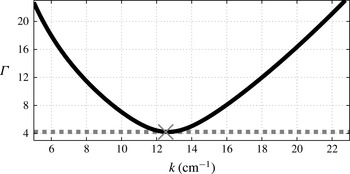
The most unstable wavenumber $k$ can then be obtained by minimizing ${\it\Gamma}$ with respect to $k$ . Figure 1 shows the curve ${\it\Gamma}(k)$ for typical values used in experiments together with a comparison to the numerically observed thresholds obtained from time-dependent simulations of the system (2.26)–(2.28).

2.3. Droplet trajectory and fluid coupling

We now proceed to the fully coupled wave–droplet model. The fluid equations, presented above, must now include the pressure forcing $P_{D}$ generated by the impacting droplet. The system takes the form

where $g(t)=g(1-{\it\Gamma}\cos ({\it\omega}_{0}t))$ .

The motion of the spherical droplet has two distinct stages, flight and impact. During flight, the droplet of mass $m$ is in ballistic motion corrected by the aerodynamic force, which may be described in terms of Stokes drag in the horizontal direction (Moláček & Bush Reference Moláček and Bush2013b ). The drop position is given by $(x,y,z)=(\boldsymbol{X}(t),Z(t))$ where $Z(t)$ is defined as the vertical position of the base of the droplet. Thus, in a frame moving with the vibrating container, the trajectory of the droplet in flight is governed by

where ${\it\mu}_{air}$ is the viscosity of air and $R_{0}$ is the drop radius. In the fluid equations, during flight, the applied surface pressure is set to zero, i.e.  $P_{D}=0$ in (2.38).

Figure 1.

Approximate Faraday subharmonic stability curve (black) as predicted by (2.35) for the experimental parameters in appendix B. The viscosity of the fluid ${\it\nu}$ was adjusted to ${\it\nu}^{\ast }=0.8025{\it\nu}$ so that the minimum of ${\it\Gamma}(k)$ , as predicted by (2.35), matches the experimental value ${\it\Gamma}=4.22$ reported in Wind-Willassen et al. (Reference Wind-Willassen, Moláček, Harris and Bush2013) and shown by the horizontal line. The minimum is achieved at $k_{F}=12.64~\text{cm}^{-1}$ . The cross indicates the numerically observed critical value for instability of (2.33), specifically $k_{\ast }=12.52~\text{cm}^{-1}$ at ${\it\Gamma}=4.22$ . The inverse Reynolds number for this case, based on ${\it\nu}^{\ast }$ , the Faraday frequency of ${\it\omega}_{0}/2$ and the associated Faraday wavelength ${\it\lambda}^{\ast }$ , is ${\it\epsilon}\approx 0.016$ .

The impact on the free surface begins at time $t=t_{I}$ when ${\it\eta}(\boldsymbol{X}(t_{I}),t_{I})=Z(t_{I})$ and $\text{d}(Z-{\it\eta})/\text{d}t|_{\boldsymbol{x}=\boldsymbol{X}}<0$ . During impact, the vertical dynamics is modelled as a nonlinear spring prescribed by the model of Moláček & Bush (Reference Moláček and Bush2013b ):

while the horizontal trajectory is given by

Details of the derivation of these equations are given in Moláček & Bush (Reference Moláček and Bush2013b ). In the equations for the vertical dynamics shown above, $\bar{{\it\eta}}$ denotes the hypothetical free-surface elevation that would exist in the absence of the current droplet impact. Thus, during the impact, two solutions to (2.38) and (2.39) are computed: the hypothetical one  $\bar{{\it\eta}},\bar{{\it\phi}}$ (where $\bar{{\it\phi}}$ is the velocity potential of this hypothetical flow) with $P_{D}=0$ and ‘initial value’ $\bar{{\it\eta}}={\it\eta}$ , $\bar{{\it\phi}}={\it\phi}$ at $t=t_{I}$ ; and another, denoted ${\it\eta},{\it\phi}$ , which does include the pressure forcing due to the drop. This second solution is not explicitly used during the current impact, but captures the wave generation that will affect subsequent impacts. We note that in previous models (Oza et al. Reference Oza, Rosales and Bush2013; Moláček & Bush Reference Moláček and Bush2013b ) the free-surface geometry is calculated without accounting for the current impact, whose effect on the wave field is included after the impact. Our model thus goes beyond its predecessors in explicitly computing the dynamic wave generation and propagation. A comparison between the waveforms predicted by the various models will be presented in § 3.3.

The constants $c_{1},c_{2},c_{3},c_{4}$ are fixed: we carry out all single droplet experiments with values similar to those used in Moláček & Bush (Reference Moláček and Bush2013b ) and Wind-Willassen et al. (Reference Wind-Willassen, Moláček, Harris and Bush2013) (see appendix B). Briefly, $c_{1}$ prescribes the spring nonlinearity, $c_{2}$ the vertical component of damping, $c_{3}$ the drop’s added mass induced during impact and $c_{4}$ the skidding friction. The right-hand side of (2.43) represents the propulsive force induced by the droplet’s impact on the inclined surface at the impact location $\boldsymbol{X}$ . This impact force $F(t)$ experienced by the droplet is extracted from the vertical dynamics equation as

The thresholding to prevent negative (suction) forces ( $F(t)<0$ ) was introduced on physical grounds in Moláček & Bush (Reference Moláček and Bush2013b ). The pressure is now given by

for $|\boldsymbol{x}-\boldsymbol{X}|<R(t)$ and $P_{D}=0$ otherwise. Here $R(t)$ denotes the contact radius, which we model as

The lower bound is the leading-order approximation of the area of the base of the spherical cap resulting from intersecting the droplet with the horizontal plane of the unperturbed free surface, and the upper bound is an approximation guided by experimental observations. In applying (2.45) we have made the further approximation that the pressure forcing is spatially uniform over the impact area. We find that the model is not sensitive to changes in these approximations.

The impact ends at $t=t_{E}$ , when $\bar{{\it\eta}}(\boldsymbol{X}(t_{E}),t_{E})=Z(t_{E})$ and $\text{d}(Z-\bar{{\it\eta}})/\text{d}t|_{\boldsymbol{x}=\boldsymbol{X}}>0$ . At $t=t_{E}$ , the ‘bar’ variables are discarded, then reinitialized at the beginning of the next impact. In summary, the evolution of $\bar{{\it\eta}}$ determines the drop dynamics, while the evolution of ${\it\eta}$ accounts for the wave generation. A verification of the consistency of our model is that ${\it\eta}(\boldsymbol{X}(t),t)\approx Z(t)$ during droplet impact, as is evident in the traces reported in figure 3.

3.1. The spectral method

An accurate spectral method is used following the strategy of writing the evolution as a single complex equation as done by Milewski & Tabak (Reference Milewski and Tabak1999) and Wang & Milewski (Reference Wang and Milewski2012). To sketch the method, consider the dimensionless form of the equations,

where the forcing pressure has been scaled with ${\it\sigma}/{\it\lambda}$ , and time with the period of the subharmonic Faraday mode, resulting in $\mathscr{G}=G+{\it\Gamma}\cos (4{\rm\pi}t)$ .

In Fourier space, equations (3.1) and (3.2) are given by

We perform the change of variables

where

The system is then easily integrated, for each $k$ , as a single linear complex equation. The part of the equation that has constant coefficients can be integrated exactly, and then the evolution of the Fourier amplitudes amounts to

In the absence of both vibration ( ${\it\Gamma}=0$ ) and pressure forcing ( $P_{D}=0$ ), no numerical integration is needed. In the presence of these effects, equation (3.7) is solved using a fourth-order Runge–Kutta method. The original variables are recovered from $\hat{u}$ by decomposing expression (3.5) into its Hermitian and skew-Hermitian parts and inverting it. As explained earlier, during contact time, the averaged free surface $\bar{{\it\eta}}$ and its slope $\boldsymbol{{\rm\nabla}}\bar{{\it\eta}}$ feed into the droplet dynamics (2.42) and (2.43) and are obtained by integrating the wave equations with $P_{D}=0$ . The vertical dynamics and trajectory ordinary differential equations (2.40)–(2.43) are also solved directly by a Runge–Kutta method, and provide the coupling pressure $P_{D}$ through (2.44) and (2.45). To model accurately the full impact, we must resolve a multiscale problem, with scales ranging from the penetration depth, of $O(0.1~\text{mm})$ , to the characteristic wavelength of the pilot wave, of $O(1~\text{cm})$ . In our single-drop computations we typically use $1024\times 1024$ Fourier modes in space.

Figure 2.

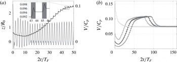
(a) Evolution of the droplet’s horizontal velocity ( $V/C_{p}$ , black) and elevation above the free surface ( $z/R_{0}$ , grey), in the bath’s frame of reference. Following its release onto the surface at a low speed, the droplet decelerates, then accelerates towards its steady walking speed. The inset shows the velocity variations over the Faraday period, reflecting the two stages of the drop motion, impact (grey) and free flight. (b) Evolution of the walker dynamics from different initial conditions. After an initial transient, all walkers converge on an identical walking state with the same impact phase.

In what follows, we present a series of numerical simulations confirming that the system of differential equations (2.38)–(2.43) is capable of generating much of the complex behaviour reported in laboratory experiments.

Figure 3.

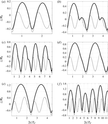
Vertical dynamics of the $(m,n)^{p}$ bouncing and walking modes: (a)  $(1,1)$ bouncing at ${\it\Gamma}=1.6$ ; (b)  $(2,2)$ bouncing at ${\it\Gamma}=2.3$ ; (c)  $(4,3)$ bouncing at ${\it\Gamma}=2.9$ ; (d)  $(2,1)^{1}$ walking at ${\it\Gamma}=3.4$ ; (e)  $(2,1)^{2}$ walking at ${\it\Gamma}=3.8$ ; and (f) chaotic walking at ${\it\Gamma}=4.15$ . The vertical position of the droplet’s lowermost point is indicated by the solid line and the height of the underlying bath by the dashed line. The panels indicate elevations relative to the non-vibrating laboratory frame of reference. The horizontal axis is in units of forcing periods ( $T_{F}=1/80~\text{s}$ ), and the vertical axis in units of drop radii. All experiments shown correspond to ${\it\Omega}=0.8$ , i.e. a drop radius of $R_{0}=0.38~\text{mm}$ forced by a bath vibrating at 80 Hz. The Faraday threshold is ${\it\Gamma}_{F}=4.22$ .

3.2. Dynamics of single drops

We first investigate the bifurcations between different walking and bouncing states as reported by Protière et al. (Reference Protière, Boudaoud and Couder2006), Eddi et al. (Reference Eddi, Terwagne, Fort and Couder2008, Reference Eddi, Sultan, Moukhtar, Fort, Rossi and Couder2011), Moláček & Bush (Reference Moláček and Bush2013a ,Reference Moláček and Bush b ) and Wind-Willassen et al. (Reference Wind-Willassen, Moláček, Harris and Bush2013). In the laboratory experiments, a droplet is released onto a vibrating bath of silicone oil. Depending on the forcing acceleration ${\it\Gamma}$ , the droplet may coalesce, bounce or walk, propelled by its own pilot wave. We proceed by comparing the experimental observations with the predictions of our model.

Following Moláček & Bush (Reference Moláček and Bush2013a ), we characterize the system in terms of the dimensionless driving acceleration, ${\it\Gamma}/{\it\Gamma}_{F}$ , and the vibration number, ${\it\Omega}$ . For given ${\it\Gamma}/{\it\Gamma}_{F}$ and ${\it\Omega}$ values, we initialize a computation by releasing a particle onto the fluid surface at a low horizontal speed. Below the walking threshold, for ${\it\Gamma}<{\it\Gamma}_{W}({\it\Omega})$ , the particle quickly comes to rest, and settles into a stationary bouncing mode. When ${\it\Gamma}>{\it\Gamma}_{W}({\it\Omega})$ the particle accelerates and settles into a steady walking state (see figure 2). Our model exhibits hysteresis, which can be observed, for example, by choosing different values of the initial particle speed. In the experiment shown in figure 2(b), the initial velocity does not affect the final steady speed. For ${\it\Omega}=0.8$ and $3.55<{\it\Gamma}<3.7$ , however, either the $(2,1)^{1}$ or $(2,1)^{2}$ state may emerge, depending on the initial velocity. Qualitatively similar hysteretic effects were observed in the experiments of Wind-Willassen et al. (Reference Wind-Willassen, Moláček, Harris and Bush2013), but not quantified. In the remainder of the paper, for simplicity, we consider only the long-time behaviour arising from low initial velocities. In certain cases, particularly when ${\it\Gamma}\approx {\it\Gamma}_{F}$ , the walking appears to be irregular and chaotic, at least over the times that we compute. We recall that our wave model has only one adjustable parameter, the effective viscosity of the fluid. Using the real viscosity of the fluid overestimates the experimental Faraday threshold by approximately 20 %. We thus adjust the viscosity in order to match this threshold (see figure 1). The parameters $c_{j}$ governing the droplet dynamics (2.42) and (2.43) are similar to those used in Moláček & Bush (Reference Moláček and Bush2013b ) and Wind-Willassen et al. (Reference Wind-Willassen, Moláček, Harris and Bush2013), but are slightly modified in order to match the experimentally observed walking threshold, ${\it\Gamma}_{W}$ (see appendix B). The walking threshold ${\it\Gamma}_{W}$ is most sensitive to the skidding friction parameter $c_{4}$ , which was chosen such that the walking threshold matched that observed experimentally. For the other parameters, the dynamics is most sensitive, in decreasing order, to $c_{1},~c_{3}$ and $c_{2}$ .

Detailed regime diagrams in the ${\it\Omega}{-}{\it\Gamma}/{\it\Gamma}_{F}$ plane were presented in Moláček & Bush (Reference Moláček and Bush2013a ,Reference Moláček and Bush b ) and Wind-Willassen et al. (Reference Wind-Willassen, Moláček, Harris and Bush2013). We adopt their nomenclature, labelling different bouncing and walking states with a triplet of integers $(m,n)^{p}$ , where $m$ is the number of forcing periods and $n$ the number of bounces in one overall bouncing cycle. If there is a multiplicity of $(m,n)$ modes, $p$ ranks them according to their relative mechanical energies, $p=1$ being the lowest. For example, $(4,2)$ signifies a motion that repeats every four forcing periods and consists of two different bounces; otherwise, it would be a $(2,1)$ mode.

In figure 3, various simulated bouncing modes are displayed. The vertical position of the lowermost point of the droplet and the free-surface elevation beneath the droplet centre are shown as a function of time for fixed ${\it\Omega}$ and several values of  ${\it\Gamma}$ . Both bouncing and walking states are represented. At a few points we note a slight inconsistency between the free-surface elevation and the droplet position during impact; specifically, the droplet appears to cross the interface. In reality, the droplet and the waves are separated by a thin lubrication layer of air that transmits normal stresses between the two. In our model, the fluid is free to respond to the pressure field of the droplet and we do not impose their relative positions. During most of the contact time, the solid and dashed lines coincide. The extent of this discrepancy, that is, the crossing of the drop and bath surfaces, thus provides a measure of the consistency of our model.

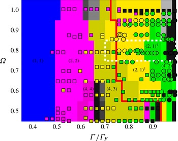
Figure 3 also indicates how the system transitions between the various modes. For example, a fundamental difference between the $(2,1)^{1}$ and $(2,1)^{2}$ modes (cf. panels d and e) is the droplet impact phase. In figure 4, the behaviour of our model is shown in the ${\it\Omega}{-}{\it\Gamma}$ plane and compared directly to the experimental results of Wind-Willassen et al. (Reference Wind-Willassen, Moláček, Harris and Bush2013) (see their figure 3). The vibration number ${\it\Omega}$ was varied in our simulations by changing the droplet radius. The predicted dynamical states are indicated by the background colour and the laboratory experiments are shown by the colour-coded points, squares for bouncers and circles for walkers. Evidently, our numerical model is able to adequately capture the diversity of bouncing modes and their transition points, with only relatively small deviations from the experimental results. The main quantitative differences are that the extent of our predicted walking region (as indicated by the red curve) is relatively large, and that the $(2,1)^{1}$ to $(2,1)^{2}$ transition occurs at a slightly higher forcing amplitude.

Figure 4.

Regime diagram indicating the form of the bouncing behaviour in the ${\it\Gamma}/{\it\Gamma}_{F}$ – ${\it\Omega}$ plane, where ${\it\Omega}={\it\omega}_{0}\sqrt{{\it\rho}R_{0}^{3}/{\it\sigma}}$ is the vibration number. Squares (bouncing modes) and circles (walking modes) are laboratory data reported by Wind-Willassen et al. (Reference Wind-Willassen, Moláček, Harris and Bush2013). The background is tiled in rectangles of size $0.1\times 0.1$ , coloured according to the $(m,n)^{p}$ mode predicted to arise at the centre of the tile. The square and round markers follow the same colour scheme as the background. The red line indicates the predicted transition between bouncing and walking predicted by our model. Black regions represent chaotic bouncing or walking, and grey regions indicate that the period of droplet motion is equal to or greater than six forcing periods. The changes in velocity and bouncing phase in the region delimited by the white dashed lines are indicated in figure 5.

Figure 5.

The dependence of impact phase ${\it\phi}$ and horizontal speed $V$ on the vibrational forcing ${\it\Gamma}/{\it\Gamma}_{F}$ for ${\it\Omega}=0.8$ , along the region delimited by the dashed white lines in figure 3. The blue line indicates $V/C_{p}$ , where $C_{p}$ is the phase speed of a wave with the Faraday wavelength. The black lines indicate the impact phase ( ${\it\phi}/2{\rm\pi}$ ). The background colours correspond to the different bouncing and walking modes, as indicated in figure 4. 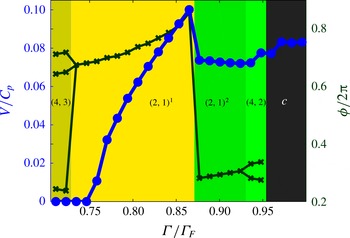For ${\it\Gamma}/{\it\Gamma}_{F}\lessapprox 0.75$ , the particle is bouncing in either the $(4,3)$ mode or the $(2,1)$ mode. The bouncer then transitions to a walking state. The phase curve takes multiple values in regimes with more than one bounce per period. A characteristic jump in both phase and speed identifies the transition between the $(2,1)^{1}$ and $(2,1)^{2}$ walking modes.

In figure 5, details of the dynamics for a horizontal slice through figure 4 at ${\it\Omega}=0.8$ are shown. Specifically, it indicates the dependence of the walking speed, impact phase and walking mode on the vibrational forcing. The impact phase and speed show a characteristic decrease at the transition between the $(2,1)^{1}$ and $(2,1)^{2}$ modes, consistent with the observations and theoretical predictions of Moláček & Bush (Reference Moláček and Bush2013b ). We recall that the variations of the drop’s walking speed, arising over the Faraday period due to its distinct phases of impact and free flight, are shown in figure 2.

Figure 6.

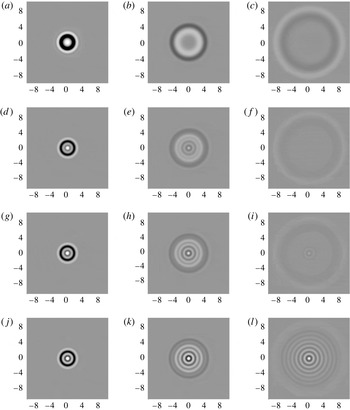
The computed wave fields generated by a single drop impact on a quiescent bath (a–c), and a bath vibrating at $f=80~\text{Hz}$ with ${\it\Gamma}=3.15$ (d–f), ${\it\Gamma}=3.6$ (g–i) and ${\it\Gamma}=4.15$ (j–l). The wave field was generated by a single impact of a drop of $R_{0}=0.38~\text{mm}$ and density 10 times that of the bath. The axes are labelled in units of Faraday wavelengths. Images are taken at times $t=2T_{F}$ (a,d,g, j), $t=6T_{F}$ (b,e,h,k) and $t=11T_{F}$ (c, f,i,l) after impact, where $T_{F}$ is the Faraday period.

Figure 7.

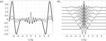
(a) Cross-sections of wave fields generated by single impact corresponding to figure 6(f) (black), (i) (grey) and (l) (light grey), normalized to have the same height at the origin. The thin line corresponds to a Bessel function $\text{J}_{0}(k_{F}r)$ . (b) Cross-sections of the single-impact free surface for ${\it\Gamma}=4.15$ at times $t=T_{F},2T_{F},\dots ,8T_{F}$ scaled so as to have the same height at the origin. The line indicates the leading edge of the disturbance. The horizontal axes show distance from the point of impact.

3.3. The walker-induced wave field

Previous theoretical models of the wave field have used a superposition of waves generated by preceding impacts,

where $h_{n}$ is the wave generated by the $n$ th prior impact at time $t_{n}$ . Two models for $h_{n}$ have been used for bouncing and walking studies. Eddi et al. (Reference Eddi, Sultan, Moukhtar, Fort, Rossi and Couder2011) proposed a cosine form with both spatial and temporal damping,

in which ${\it\delta}$ is a decay length parameter. They also introduce a Bessel function model for the surface evolution. Moláček & Bush (Reference Moláček and Bush2013b ) derived a form valid in the small-drop limit,

where the memory parameter $M_{e}=T_{d}/T_{F}(1-{\it\Gamma}/{\it\Gamma}_{F})$ depends on the proximity to threshold, as well as the decay time of the unforced waves, $T_{d}$ . We note that a memory parameter does not arise in our formulation, since we solve explicitly for the full wave field. However, an asymptotic value for the decay rate in our model, from which one may infer an analogue to the memory parameter, is provided in appendix A. The $\sqrt{t}$ decay factor arising in the narrow-band asymptotic analysis of Moláček & Bush (Reference Moláček and Bush2013b ) is omitted in some other models of the surface waves (e.g. Oza et al. Reference Oza, Rosales and Bush2013) for the sake of simplicity. Asymptotic values for the amplitude parameter $A$ and damping time $T_{d}=T_{F}M_{e}$ appearing in (3.10) are given in Moláček & Bush (Reference Moláček and Bush2013b ).

Figure 6 illustrates the numerically predicted wave fields generated by a drop impacting the surface in the absence and presence of vibrational forcing. It may be compared directly to the wave fields reported in figure 4 of Eddi et al. (Reference Eddi, Sultan, Moukhtar, Fort, Rossi and Couder2011). In the absence of vibrational forcing, a transient wave sweeps radially outwards from the point of impact. With vibrational forcing, this transient serves to trigger a standing field of Faraday waves that persists in its wake, decaying with time. In the forced experiments, both the transient wave speed and the spatial form of the excited standing wave are independent of the vigour of the vibrational forcing. The spatial form is very close to the Bessel function $\text{J}_{0}(k_{F}r)$ , particularly for later times (see figure 7). The measured speeds of the sweeping front for the experiments shown in figure 6 are $18.59$ , $19.45$ , $19.73$ and $20.04~\text{cm}~\text{s}^{-1}$ for ${\it\Gamma}=0$ , $3.15$ , $3.6$ and $4.15$ , respectively. For the cases with vibrational forcing, the speed is very close to the Faraday phase speed of $20.07~\text{cm}~\text{s}^{-1}$ . For the unforced experiment, the speed is somewhat less, and is set by least slowly damped waves excited by the impact. In this case, the speed is bounded below by the minimum gravity–capillary wave speed, $\sqrt{2}({\it\sigma}g/{\it\rho})^{1/4}\approx 17.1~\text{cm}~\text{s}^{-1}$ .

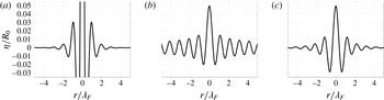
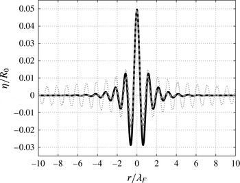
Figure 8 shows the cross-sectional free-surface height of a $(2,1)^{1}$ bouncer at the moment before impact, as predicted by a number of theoretical models. Figure 9 shows a comparison between our numerical wave profile, and the Bessel approximations of Moláček & Bush (Reference Moláček and Bush2013b ) without and with a spatial damping term. The spatial damping follows from expression (3.10) due to Moláček & Bush (Reference Moláček and Bush2013b ) (see their equations (A46) for ${\it\beta}_{1}$ and (A47)), which has an $O(r^{2}/4{\it\beta}_{1}{\it\tau})$ correction term arising from an expansion of $\exp (-r^{2}/4{\it\beta}_{1}{\it\tau})$ . When this correction is applied, each Bessel function is multiplied by a Gaussian radial profile. These results highlight the role of exponential spatial decay on the walker’s wave field.

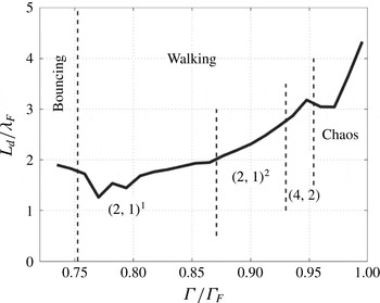
In figure 10, we show the dependence of the spatial decay length of the bouncers and walkers on ${\it\Gamma}$ , as computed by factoring out the $r^{-1/2}$ spatial decay factor of the $\text{J}_{0}(k_{F}r)$ Bessel function. Specifically, we took the modulus of every maximum and minimum transverse to the walking direction and fitted it to a curve of the form $Ar^{-1/2}\exp (-r/L_{d})$ . The spatial decay length increases between $1.5{\it\lambda}_{F}$ and $4{\it\lambda}_{F}$ as ${\it\Gamma}$ is increased progressively. We note that the only experimental spatial decay length reported in the literature is the $1.6{\it\lambda}_{F}$ mentioned by Eddi et al. (Reference Eddi, Sultan, Moukhtar, Fort, Rossi and Couder2011).

Figure 8.

Different model predictions of the free-surface cross-section of a $(2,1)^{1}$ bouncer at the moment before impact with ${\it\Gamma}=3.1$ . (a) The cosine wave model (3.9) of Eddi et al. (Reference Eddi, Sultan, Moukhtar, Fort, Rossi and Couder2011) with a spatial damping with decay length $1.6{\it\lambda}_{F}$ reported by the authors. Note the singularity at $r=0$ . (b) The Bessel model (3.10) of Moláček & Bush (Reference Moláček and Bush2013b ). (c) The result of our computation.

Figure 9.

Comparison between the wave-field predictions of the present model (black curve) with those of Moláček & Bush (Reference Moláček and Bush2013b ) without (dotted curve) and with (grey dashed curve) the higher-order spatial damping correction suggested by Moláček & Bush (Reference Moláček and Bush2013b ) to the Bessel model (3.10).

Figure 10.

Computed dependence of the dimensionless decay length ( $L_{d}/{\it\lambda}_{F}$ ) on the vibrational forcing ${\it\Gamma}$ . Here, ${\it\Omega}=0.8$ . As ${\it\Gamma}$ is increased, the bouncer evolves into a walker with the gaits indicated.

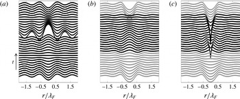
Figure 11 shows the time evolution of the free surface arising from the same $(2,1)^{1}$ bouncer as in figure 8 over the course of a Faraday period. While the Bessel model is constructed as a standing wave, our solution clearly generates a wave that propagates away from the impact centre as evidenced by the V-shaped furrow in figure 11(b,c). We note that the full temporal wave field of the Bessel approximation has been used in a variety of situations, for example, in chaotic bouncing (Moláček & Bush Reference Moláček and Bush2013b ).

Figure 11.

The time evolution of the free surface through the course of a Faraday period for the same bouncer as in figure 8. (a) The model of Moláček & Bush (Reference Moláček and Bush2013b ), as described by equation (3.10). The discontinuity arises when the surface is updated by the addition of a new Bessel function. (b) Our model’s prediction, $\bar{{\it\eta}}$ , for the free surface in the absence of the current impact. The dark curves correspond to wave forms arising when the drop is in contact with the bath, the lighter curves to times when the drop is in flight. (c) Our model prediction for the free surface when the current droplet impact is included.

Figure 12.

(a) The Doppler effect arising at ${\it\Omega}=0.8,~{\it\Gamma}=3.6$ . The solid line shows the surface along the direction of motion, the dashed line that in the transverse direction. The horizontal axis is in units of Faraday wavelengths, and the vertical axis in units of drop radii. (b) The Doppler effect displayed ahead and behind the walker, with ${\it\lambda}/{\it\lambda}_{F}$ (vertical axis) in terms of $V/C_{p}$ . The $\times$ markers depict the wavelength ahead of the walker, the $+$ markers the wavelength behind it. The lines indicate the magnitude of the Doppler effect reported by Eddi et al. (Reference Eddi, Sultan, Moukhtar, Fort, Rossi and Couder2011). Here $V$ is the mean walker speed and $C_{p}$ the phase speed.

Figure 13.

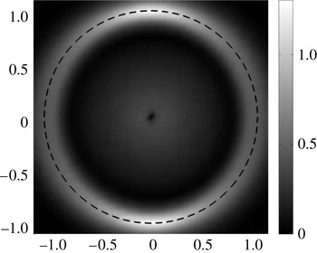
Amplitude of the Fourier spectrum of the computed wave field for a walker immediately before the drop impacts the surface. A superposition of Bessel functions $\text{J}_{0}(k_{F}r)$ would have a spectrum only on the dashed circle of radius $k_{F}$ . It is the frequency spread of the spectrum about this circle that allows for a Doppler shift in the wave field. Axes are in units of inverse Faraday wavelengths.

The Doppler shift along a walker’s wave field is displayed in figure 12(a). The solid line shows the free surface along the direction of motion, and the dashed line that in the transverse direction. The Doppler shifting is evidenced by the changing distance between crests on the two curves. Figure 12(b) shows the dependence of the Doppler shift on the walker’s mean velocity, along with the experimental results of Eddi et al. (Reference Eddi, Sultan, Moukhtar, Fort, Rossi and Couder2011). While the Bessel-function-based models have been successful in describing certain aspects of the problem, they cannot capture the Doppler shift due to the moving wave maker. This arises from the fact that the Bessel function $\text{J}_{0}(k_{F}r)$ can be written as the superposition of plane cosines of fixed wavelength $2{\rm\pi}/k_{F}$ in every direction, centred at the origin:

Therefore the function $\text{J}_{0}(k_{F}r)$ in the $(x,y)$ plane does not contain wavelengths other than $2{\rm\pi}/k_{F}$ . Physically, this is the wavelength observed in all directions as $r$ becomes large. Alternatively, the spectrum $\hat{\text{J}}_{0}(\boldsymbol{k}/k_{F})$ is non-zero only on the circle $k=k_{F}$ in the $(k_{1},k_{2})$ plane.

The free-surface elevation of a $(2,1)$ walker with straight-line trajectory $\boldsymbol{X}=(V(t-{\it\phi}),0)$ with impacts at $t_{n}=-2nT_{f}+{\it\phi}$ and observed immediately before an impact at $t={\it\phi}$ is

Its Fourier transform is given by

where $\hat{\text{J}}$ is the Fourier transform of $\text{J}$ , and $\boldsymbol{k}=(k_{1},k_{2})$ . This formula shows that according to this Bessel-function model, the spectrum of the full wave field is equal to the spectrum of the single Bessel function $\text{J}_{0}(k_{F}r)$ multiplied by a function of $k_{1}$ . The wave field thus contains energy only at the wavelength $2{\rm\pi}/k_{F}$ , and the mathematical form (3.12) cannot capture a Doppler shift. Figure 13 shows the Fourier spectrum of the numerical wave field for a walker immediately before the drop strikes the surface. By way of comparison, the spectrum of (3.12) would lie only on the circle in the figure.

Figure 14.

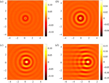
Wave fields accompanying bouncing and walking drops. (a) At ${\it\Gamma}=3.1$ , the axisymmetric wave field of a bouncer arises. At (b)  ${\it\Gamma}=3.3$ , (c)  ${\it\Gamma}=3.8$ and (d)  ${\it\Gamma}=4.15$ , walkers of progressively increasing speed arise, their wave fields being progressively more fore–aft asymmetric. Axes are in units of Faraday wavelengths, and the surface elevation (side bar) is in units of drop radii. In all panels, the drop is at the origin and (except for a) moving to the right. The simulations were performed with drops of ${\it\Omega}=0.8$ (i.e.  $R_{0}=0.38~\text{mm}$ ), for ${\it\Gamma}_{W}=3.15$ .

Finally, typical wave fields computed from our single-droplet simulations are shown in figure 14. These are consistent with the laboratory images presented in Eddi et al. (Reference Eddi, Sultan, Moukhtar, Fort, Rossi and Couder2011), as well as the stroboscopic model predictions of Oza et al. (Reference Oza, Rosales and Bush2013). Figure 14(d) shows that, when the walker moves rapidly to the right, an interference pattern appears in its wake.

3.4. Two-particle interaction

The generalization of our model to numerous walkers is straightforward, so we do not present it in detail. The additional ingredient is the computation of a mean free-surface elevation $\bar{{\it\eta}}_{j}$ for each particle during the fluid impact. This elevation incorporates the waves due to the impact of all other particles. Hence, in computing $\bar{{\it\eta}}_{j}$ , we take the pressure in (2.38) to be

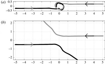
We proceed by investigating the interaction between a pair of walkers, as was examined experimentally by Protière et al. (Reference Protière, Boudaoud and Couder2006), Protière, Bohn & Couder (Reference Protière, Bohn and Couder2008) and Eddi et al. (Reference Eddi, Moukhtar, Perrard, Fort and Couder2012). We confine our attention to two special cases, where the walkers are initially antiparallel and parallel. Protière et al. (Reference Protière, Bohn and Couder2008) report that when the walkers are initially antiparallel, and so approach each other, they may either scatter or lock into orbit, depending on their relative bouncing phase, and the perpendicular distance between their original paths, the so-called impact parameter,  $d_{I}$ .

Figure 15.

Collisions of in-phase droplet pairs. (a) With impact parameter of $d_{I}=0.5{\it\lambda}_{F}$ , the pair are captured in a periodic orbit with a diameter of approximately $0.5{\it\lambda}_{F}$ . (b) With an impact parameter $d_{I}={\it\lambda}_{F}$ , the droplets scatter. Vertical and horizontal length scales are in units of ${\it\lambda}_{F}$ .

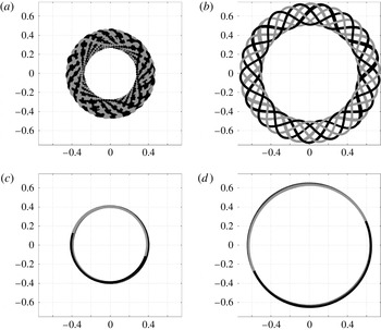
In the scattering regime, wave forces on the droplets causes them to repel. Conversely, in the orbiting regime, the droplet pair forms a stable and well-defined association bound together by their superposed pilot waves. In figure 15, orbiting and scattering of in-phase droplets are shown. Orbital states obtained by varying ${\it\Gamma}$ for in- and out-of-phase walkers are shown in figure 16. The orbits are stable (i.e. persistent after extended computations) and can have different forms (circular, periodic wobbling or chaotic wobbling) depending on the system parameters, particularly the forcing amplitude ${\it\Gamma}$ . Note that the in-phase orbiters have an orbital diameter of approximately $0.8{\it\lambda}_{F}$ ; the out-of-phase orbiters approximately $1.3{\it\lambda}_{F}$ . This difference may be roughly understood on the grounds that orbiters are more stable when bouncing in the troughs than on the crests of their partner’s wave field.

Figure 16.

Orbital modes arising through walker–walker interactions, specifically from a pair of identical walkers launched with antiparallel velocity. Bouncing in phase with (a)  $c_{4}=0.32$ , ${\it\Omega}=0.8$ , ${\it\Gamma}=3.7$ and (c)  $c_{4}=0.3$ , ${\it\Omega}=0.7$ , ${\it\Gamma}=4$ . Bouncing out of phase with (b)  $c_{4}=0.32$ , ${\it\Omega}=0.8$ , ${\it\Gamma}=3.6$ and (d)  $c_{4}=0.3$ , ${\it\Omega}=0.7$ , ${\it\Gamma}=4$ . Axes are in units of the Faraday wavelength. Note the offset of orbital radii between the in- and out-of-phase walkers.

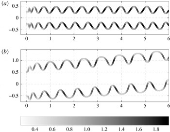
When the walkers are initially parallel, they may lock into a ‘promenade mode’, in which they walk in unison, but the distance between them oscillates periodically (figure 17). After an initial transient, a well-defined periodically oscillating walking state emerges. This promenade mode and the characteristic oscillations in speed are both readily observed in the laboratory, and have recently been investigated by Borghesi et al. (Reference Borghesi, Moukhtar, Labousse, Eddi, Fort and Couder2014).

Figure 17.

Droplet pair forming a stable ‘promenade mode’. Two identical droplets propagate together in a given direction while oscillating in the transverse direction. Axes are in units of the Faraday wavelength. Two walkers bouncing (a) in phase and (b) out of phase. The instantaneous speed $V/C_{p}$ is colour-coded according to the grey scale bar. The mean speeds of the promenading pair in panels (a) and (b) are 0.88 and 0.63 of the single-walker free walking speed, respectively.