1 Introduction
The fluid mechanics of water-entering objects is of enormous importance in many military and industrial processes, resulting in many studies over the last few decades (Abelson Reference Abelson1970; May Reference May1975; Abrate Reference Abrate2013). In particular, the water-entry dynamics up to pinch-off has been extensively studied in terms of air-cavity shapes, perturbed fluid flows and pinch-off behaviours (Bergmann et al. Reference Bergmann, Van Der Meer, Stijnman, Sandtke, Prosperetti and Lohse2006; Duclaux et al. Reference Duclaux, Caillé, Duez, Ybert, Bocquet and Clanet2007; Gekle et al. Reference Gekle, Gordillo, Van der Meer and Lohse2009a ,Reference Gekle, Snoeijer, Lohse and Van der Meer b ; Truscott & Techet Reference Truscott and Techet2009). However, the long-term stability of the air cavity after pinch-off has drawn less attention so far.
The elongation and pinch-off of the air cavity is a dynamic interplay between surface tension, gravity and inertia (Truscott, Epps & Beden Reference Truscott, Epps and Beden2014). After the air cavity has formed, hydrostatic pressure pushes the air/liquid interface radially inward, which eventually causes the cavity to collapse resulting in a distinct pinch-off or the deep seal event (May Reference May1952). By placing probes (housing piezo-electric pressure transducers) under water to measure the cavity pressure gradient, Abelson (Reference Abelson1970) showed that pinch-off causes a sudden increase of pressure inside the air cavity, which results in the formation of damped pressure oscillations inside the cavity. To our knowledge, only a few studies have investigated the long-term cavity dynamics after pinch-off, in which ripples form along the air cavity (Grumstrup, Keller & Belmonte Reference Grumstrup, Keller and Belmonte2007; Bodily, Carlson & Truscott Reference Bodily, Carlson and Truscott2014; Mansoor et al. Reference Mansoor, Marston, Vakarelski and Thoroddsen2014). Grumstrup et al. (Reference Grumstrup, Keller and Belmonte2007) showed for the first time that the ripples originate from acoustic pressure. A few years later, Mansoor et al. (Reference Mansoor, Marston, Vakarelski and Thoroddsen2014) investigated the air cavity dynamics following hydrophobic spheres without surface seals. Depending on the speed, they observed the surface undulation of the air cavity which led to multiple pinch-off locations. Similar to Grumstrup et al. (Reference Grumstrup, Keller and Belmonte2007), pressure perturbations were found following pinch-off. The same year, Bodily et al. (Reference Bodily, Carlson and Truscott2014) investigated the water entry of slender axisymmetric bodies and noticed the formation of ripples of the same frequency found by Grumstrup et al. (Reference Grumstrup, Keller and Belmonte2007).
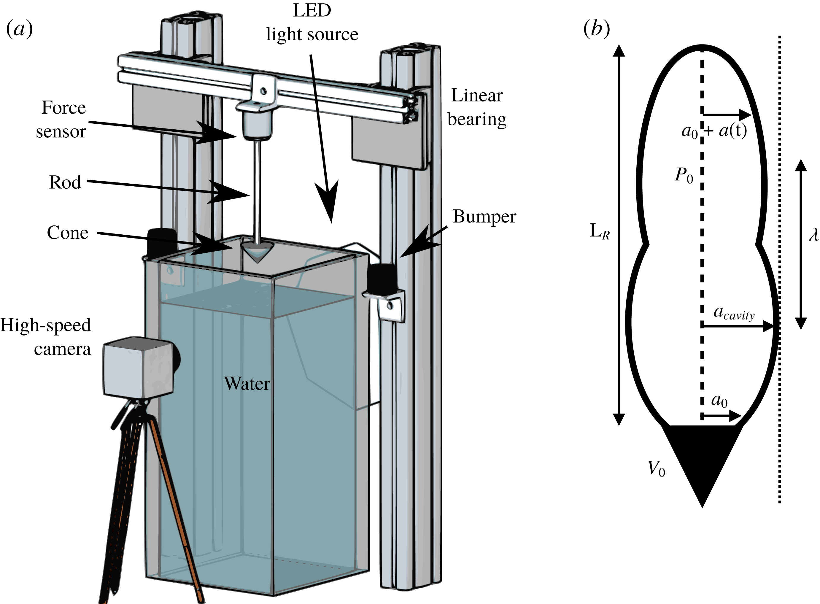
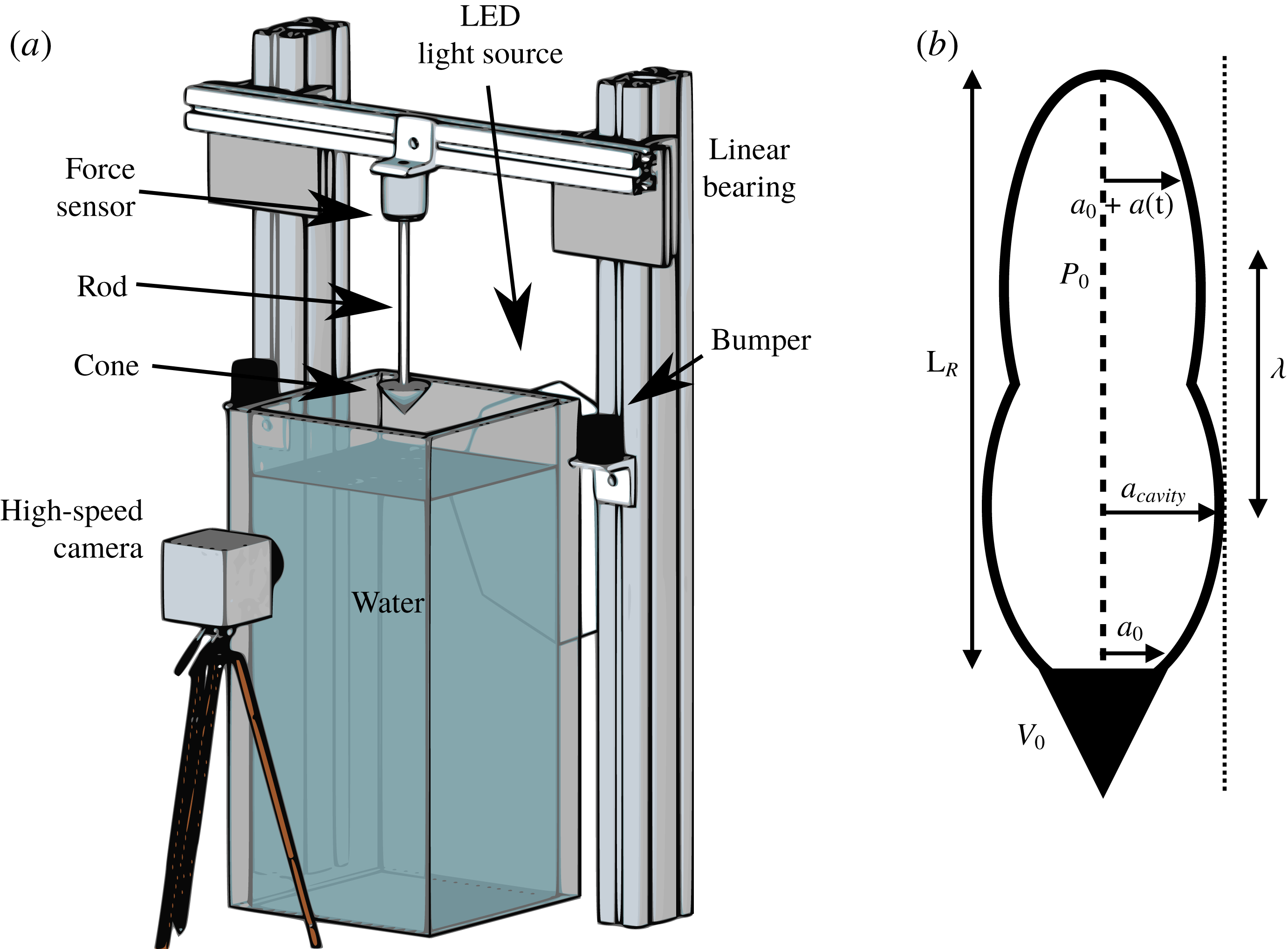
In this paper, we investigate the long-term dynamics of an air cavity that remains attached to a cone (see set-up in figure 1 a). We especially focus on the ripple formation after the pinch-off and the force associated with the ripples. In § 2, We develop an acoustic model, similar to Grumstrup et al. (Reference Grumstrup, Keller and Belmonte2007), predicting the ripple wavelength and compare it with the optically measured wavelengths of the air cavity. We then combine the experimentally measured wavelength with the acoustic model to estimate the force acting on the cone that originates from the ripples. We found a close in-phase relationship between our estimated force acting on the cone from the model and the experimentally measured force. This suggests that the ripples in the force signal are of acoustic origin. These results and the experimental set-up are displayed in § 3. Finally, we summarize the results and discuss the future direction in § 4.
2 Theory for ripple formation
After pinch-off, the radius of the air cavity undulates with time (Grumstrup et al. Reference Grumstrup, Keller and Belmonte2007). To understand the ripple shape and motion, we first make two assumptions: (i) the initial radius of an air cavity is the same as the cone radius, and (ii) the flow around the cavity is irrotational (Epstein & Keller Reference Epstein and Keller1972; Grumstrup et al. Reference Grumstrup, Keller and Belmonte2007).
We thus take the acoustic wave equation with the velocity potential
 $\unicode[STIX]{x1D6F7}(r,t)$
in a cylindrical coordinate system
 $$\begin{eqnarray}\displaystyle \unicode[STIX]{x1D6F7}_{rr}+\frac{1}{r}\unicode[STIX]{x1D6F7}_{r}=\frac{1}{c^{2}}\unicode[STIX]{x1D6F7}_{tt}, & & \displaystyle\end{eqnarray}$$
where
 $c$
is the speed of sound in water (
 $=1482~\text{m}~\text{s}^{-1}$
), and subscripts denote derivatives. We also take the Bernoulli equation as
 $$\begin{eqnarray}\displaystyle P(r,t)=P_{0}-\unicode[STIX]{x1D70C}\left(\unicode[STIX]{x1D6F7}_{t}+{\textstyle \frac{1}{2}}\unicode[STIX]{x1D6F7}_{r}^{2}\right), & & \displaystyle\end{eqnarray}$$
where
 $\unicode[STIX]{x1D70C}$
is the density of water and
 $P_{0}$
is the ambient pressure. At an interface with small-amplitude ripples, the radius is expressed as
 $r=a_{0}+a(t)$
, where
 $a_{0}$
is the initial radius of the cavity. Now, following Epstein & Keller (Reference Epstein and Keller1972) (see appendix A for details), the Bernoulli equation can be linearized to
 $$\begin{eqnarray}\displaystyle P_{r}|_{r=a_{0}}\,a(t)=-\unicode[STIX]{x1D70C}\,\unicode[STIX]{x1D6F7}_{t}. & & \displaystyle\end{eqnarray}$$
The boundary condition for the radial velocity is expressed as
 $$\begin{eqnarray}\displaystyle a_{t}=\unicode[STIX]{x1D6F7}_{r}|_{r=a(t)}, & & \displaystyle\end{eqnarray}$$
and the average pressure in the air cavity (polytropic gas law) is expressed as
 $$\begin{eqnarray}\displaystyle \bar{P}(a(t),t)=P(a_{0})\left[\frac{a_{0}^{2}L_{r}}{\displaystyle \int ^{L_{r}}(a_{0}+a(t))^{2}\,\text{d}z}\right]^{\unicode[STIX]{x1D705}}, & & \displaystyle\end{eqnarray}$$
at the air–water interface. Here,
 $\unicode[STIX]{x1D705}$
is the adiabatic exponent of air (
 ${\approx}1.4$
),
 $L_{r}$
the length of the ripple and
 $P(a_{0})$
is assumed to be the atmospheric pressure
 $P_{0}$
(see schematic in figure 1
b).
(a) Schematic of the experimental set-up. A cone is attached to a rigid rod, whose tip is at a distance
 $H_{0}$
from the water free surface of the tank. A force sensor is attached at the other extremity of the rod and fixed on a beam connected to two
 $80/20$
linear bearings that only allow a vertical displacement. A high-speed camera (Photron Fastcam Mini UX100) records the cone displacement and the air-cavity shapes. (b) Schematic of a cone and the air cavity trailing behind it.
By solving (2.1) by separation of variables, we get the solution for a velocity potential as
 $$\begin{eqnarray}\displaystyle \unicode[STIX]{x1D6F7}(r,t)=B\,\text{K}_{0}\left(\frac{\unicode[STIX]{x1D714}}{c}r\right)\text{e}^{-\unicode[STIX]{x1D714}t}, & & \displaystyle\end{eqnarray}$$
where
 $\text{K}_{0}$
is the modified Bessel function of the second kind of order zero,
 $B$
is a constant of integration and
 $\unicode[STIX]{x1D714}$
the frequency. Using the above velocity potential as a solution for the linearized Bernoulli equation (2.3) yields the amplitude of an air cavity, expressed as
 $$\begin{eqnarray}\displaystyle a(t)=A\text{e}^{-\unicode[STIX]{x1D714}t},\quad \text{with}~A=B\,\frac{\unicode[STIX]{x1D70C}\unicode[STIX]{x1D714}}{P_{r}|_{r=a_{0}}}\,\text{K}_{0}\left(\frac{\unicode[STIX]{x1D714}}{c}a_{0}\right). & & \displaystyle\end{eqnarray}$$
Plugging (2.6) and (2.7) into the kinematic boundary condition from (2.4), we get the dispersion relation as
 $$\begin{eqnarray}\displaystyle \unicode[STIX]{x1D714}^{2}\text{K}_{0}\left(\frac{\unicode[STIX]{x1D714}}{c}a_{0}\right)=\frac{\unicode[STIX]{x1D714}}{\unicode[STIX]{x1D70C}c}P_{r}|_{r=a_{0}}\,\text{K}_{1}\left(\frac{\unicode[STIX]{x1D714}}{c}a_{0}\right). & & \displaystyle\end{eqnarray}$$
In the limit of large
 $\unicode[STIX]{x1D714}$
, and by using an asymptotic expansion of the modified Bessel function of the second kind to get
 $\text{K}_{0}(x)=(\unicode[STIX]{x03C0}/2x)^{1/2}\text{e}^{-x}(1-1/8x+\cdots )$
and
 $\text{K}_{1}(x)=-\unicode[STIX]{x2202}\text{K}_{0}(x)/\unicode[STIX]{x2202}x=(\unicode[STIX]{x03C0}/2x)^{1/2}\text{e}^{-x}(1+3/8x+\cdots \,)$
, the previous dispersion relation becomes
 $$\begin{eqnarray}\displaystyle \unicode[STIX]{x1D714}^{2}=P_{r}|_{r=a_{0}}\,\frac{\unicode[STIX]{x1D714}}{\unicode[STIX]{x1D70C}c}\left(1+\frac{c}{2\unicode[STIX]{x1D714}a_{0}}\right). & & \displaystyle\end{eqnarray}$$
Detailed derivations are presented in appendix B. The solution for the above quadratic equation is
 $\unicode[STIX]{x1D714}=-\unicode[STIX]{x1D714}_{r}\pm \text{i}\unicode[STIX]{x1D714}_{i}$
, where
 $$\begin{eqnarray}\displaystyle \unicode[STIX]{x1D714}_{r} & = & \displaystyle -\frac{P_{r}|_{r=a_{0}}}{2\unicode[STIX]{x1D70C}c}=\frac{\unicode[STIX]{x1D705}P_{0}}{\unicode[STIX]{x1D70C}ca_{0}},\end{eqnarray}$$
 $$\begin{eqnarray}\displaystyle \unicode[STIX]{x1D714}_{i} & = & \displaystyle \sqrt{\frac{-P_{r}|_{r=a_{0}}}{2\unicode[STIX]{x1D70C}a_{0}}-\left(\frac{P_{r}|_{r=a_{0}}}{2\unicode[STIX]{x1D70C}c}\right)^{2}}=\sqrt{\frac{\unicode[STIX]{x1D705}P_{0}}{\unicode[STIX]{x1D70C}a_{0}^{2}}-\left(\frac{\unicode[STIX]{x1D705}P_{0}}{\unicode[STIX]{x1D70C}a_{0}c}\right)^{2}},\end{eqnarray}$$
where
 $P_{r}|_{r=a_{0}}$
is calculated to be
 $-2\unicode[STIX]{x1D705}P_{0}/a_{0}$
using the polytropic law in a cylindrical air cavity. Here,
 $\unicode[STIX]{x1D714}_{r}$
is the damping rate and
 $\unicode[STIX]{x1D714}_{i}$
is the frequency of the oscillatory mode. Our expression for
 $\unicode[STIX]{x1D714}_{i}$
is a correction of the expression in Grumstrup et al. (Reference Grumstrup, Keller and Belmonte2007) where a prefactor ‘2’ is present on the numerators.
By estimating the wavelength
 $\unicode[STIX]{x1D706}=2\unicode[STIX]{x03C0}V_{0}/\unicode[STIX]{x1D714}_{i}$
with (2.11), we predict a normalized wavelength
 $\unicode[STIX]{x1D706}/a_{0}\approx 0.53V_{0}$
regardless of the cone angle, where
 $V_{0}$
is the cone velocity.
3 Experimental results
3.1 Experimental set-up and procedure
A schematic of the experiment is presented in figure 1(a). A cone of radius
 $a_{0}~(=1.9\pm 0.1~\text{cm})$
is attached to the bottom of a thin rod (radius
 ${\approx}$
0.3 cm). The cone is made of poly-actic acid (PLA) plastic using a 3D printer (MakerBot Replicator +). The rod is mounted to the centre of the cone, and does not affect the global flow and cavity dynamics significantly. The top part of the rod is connected to a force sensor (Omega Engineering Inc., Model LC105-25,
 $3~\pm 0.0075~\text{mV}~\text{V}^{-1}$
) which measures the hydrodynamic force applied to the cone. The cone–rod system is placed at a distance
 $H_{0}$
above the water surface. While the cone is held in position above the water, the signal from the force transducer is zeroed. It is held in position using a rope held by the experimenter which is suddenly released to drop the cone–rod system into a large tank filled with water (
 $50\times 50\times 130~\text{cm}^{3}$
). The cone falls from the height
 $H_{0}$
, hits the water and continues to descend until the rod hits a bumper. This system is based on a driven fall. The cone speed linearly increases over time, whose acceleration is less than one gravity. An offset in the force measurements accounts for the acceleration, which is subtracted in the later force analysis.
The trajectory of the cone is recorded using a high-speed camera (Photron Fastcam Mini UX100) at 1000 f.p.s., which allows us to precisely track the position of the cone and the interface of the air cavity. We can thus accurately extract the cone velocity profile, and determine the pinch-off time and location (with an accuracy of
 $\pm$
1 ms, and
 $\pm$
0.3 cm). Experiments are performed with five different cone angles (
 $\unicode[STIX]{x1D703}=25^{\circ }$
,
 $45^{\circ }$
,
 $60^{\circ }$
,
 $90^{\circ }$
and
 $116^{\circ }$
) and six different dropping heights (
 $H_{0}=10$
, 20, 30, 40, 50 and 60 cm, at
 $\pm$
0.1 cm). The speed of the cone at pinch-off,
 $V$
, varies from 2.4 to
 $4.2~\text{m}~\text{s}^{-1}$
, resulting in a Froude number
 $Fr=V^{2}/(ga_{0})$
(
 $g$
is the gravitational acceleration, and
 $a_{0}$
is the cone radius) ranging between 30 and 90. Later, values of Froude numbers from individual tests will be used. We performed 5 trials at a given height and cone angle, and also developed a MATLAB code to analyse the data. This code gives us the amplitudes and wavelengths optically measured from pictures, with a pix/mm resolution between 1 and 3, depending on the trials. Similarly, the resolution for the amplitudes and wavelengths from the force sensor is given by the force sensor resolution (between 0.01 and 0.2 N).
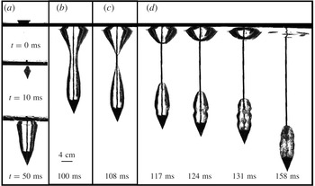
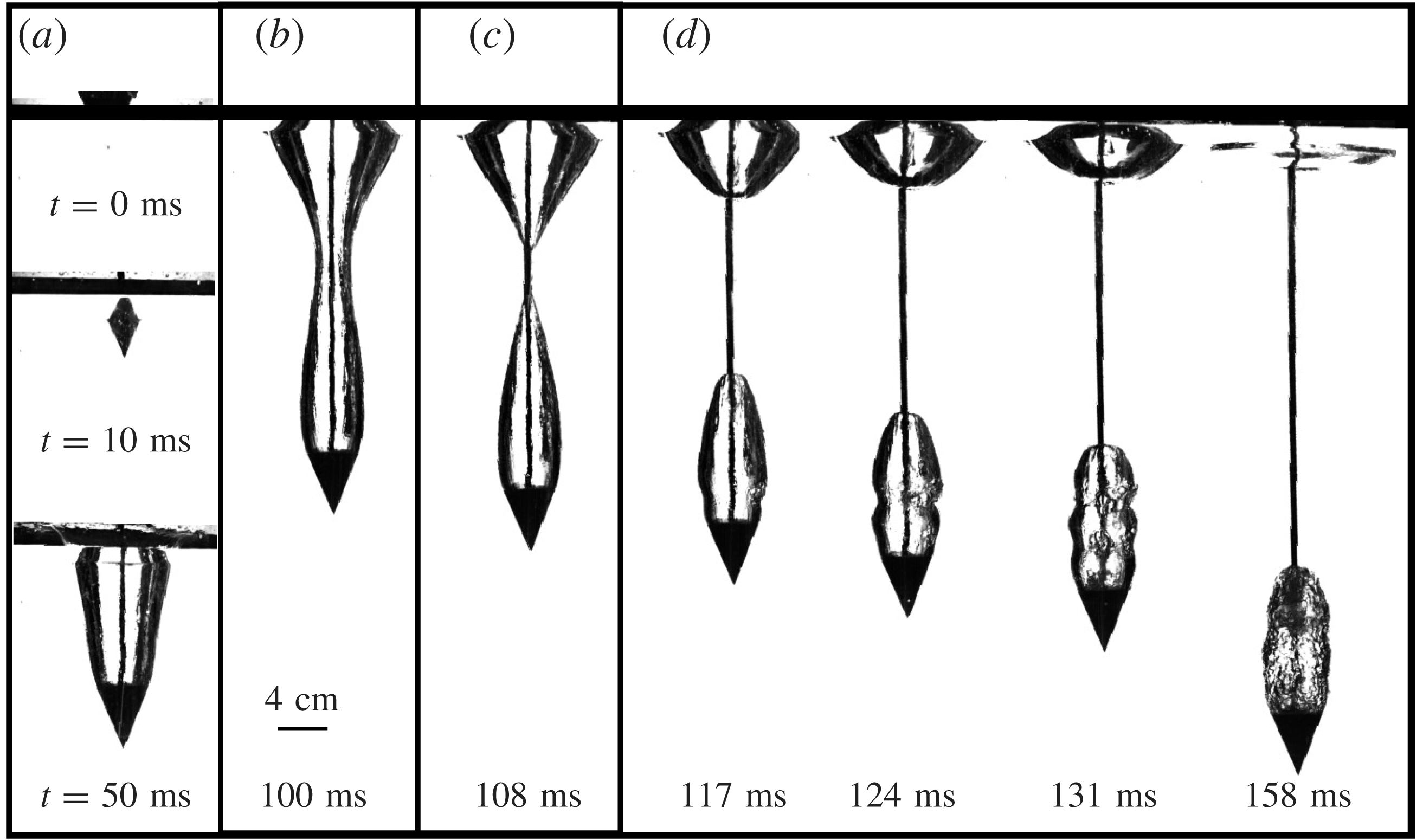
Snapshots from an experimental run for a cone with a 2 cm radius and
 $45^{\circ }$
cone angle impacting at
 $3.30~\text{m}~\text{s}^{-1}$
. The reference time of
 $t=0$
s is when the cone impacts the water. (a) Within a few milliseconds the cone penetrates the water and drags an air cavity. (b) After a few tens of milliseconds, the cavity radius decreases until it collapses (pinch-off), as shown in (c). (d) After pinch-off the propagation of an acoustic wave generates ripples at the air–water interface.
3.2 Observations
Experimental snapshots of the air cavity with a
 $45^{\circ }$
cone angle and at a velocity of
 $3.30~\text{m}~\text{s}^{-1}$
is shown in figure 2. We observed that an air cavity was dragged by the cone and pinches off at approximately 108 ms. Ripples were formed at the interface just after pinch-off (see figure 2
d), and disappeared at the moment when the cone–rod system stops descending after hitting the safety bump at around 160 ms. The dynamics of these ripples is governed by the acoustic wave generated during the closing of the air cavity (Grumstrup et al.
Reference Grumstrup, Keller and Belmonte2007). This is in contrast to the dynamics of ventilated supercavity pulsations which is driven by the underlying thermodynamics (Franc & Michel Reference Franc and Michel2006).
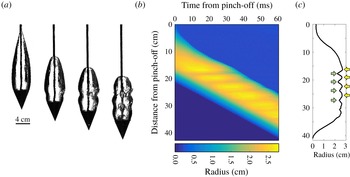
The images shown here are presented for the same experiment done with a cone angle of
 $45^{\circ }$
and an impact speed of
 $3.30~\text{m}~\text{s}^{-1}$
. (a) Typical images obtained from the high-speed camera (Fastcam Mini UX100) at a frame rate of 1000 f.p.s. The first image is showing when pinch-off is occurring (
 $t=0$
ms). After that, at
 $t=9$
ms, we can see the first ripple. The third and fourth images are taken 7 ms later, at respectively
 $t=16$
ms and
 $t=23$
ms. (b) Spatio-temporal plot where the distance from the pinch-off location is plotted as a function of the time from pinch-off. The brighter areas correspond to the ripples. (c) Maximum width extracted from a spatio-temporal plot like (b). The yellow and green arrows are respectively indicating the maximal and minimal value of the radius of the air cavity.
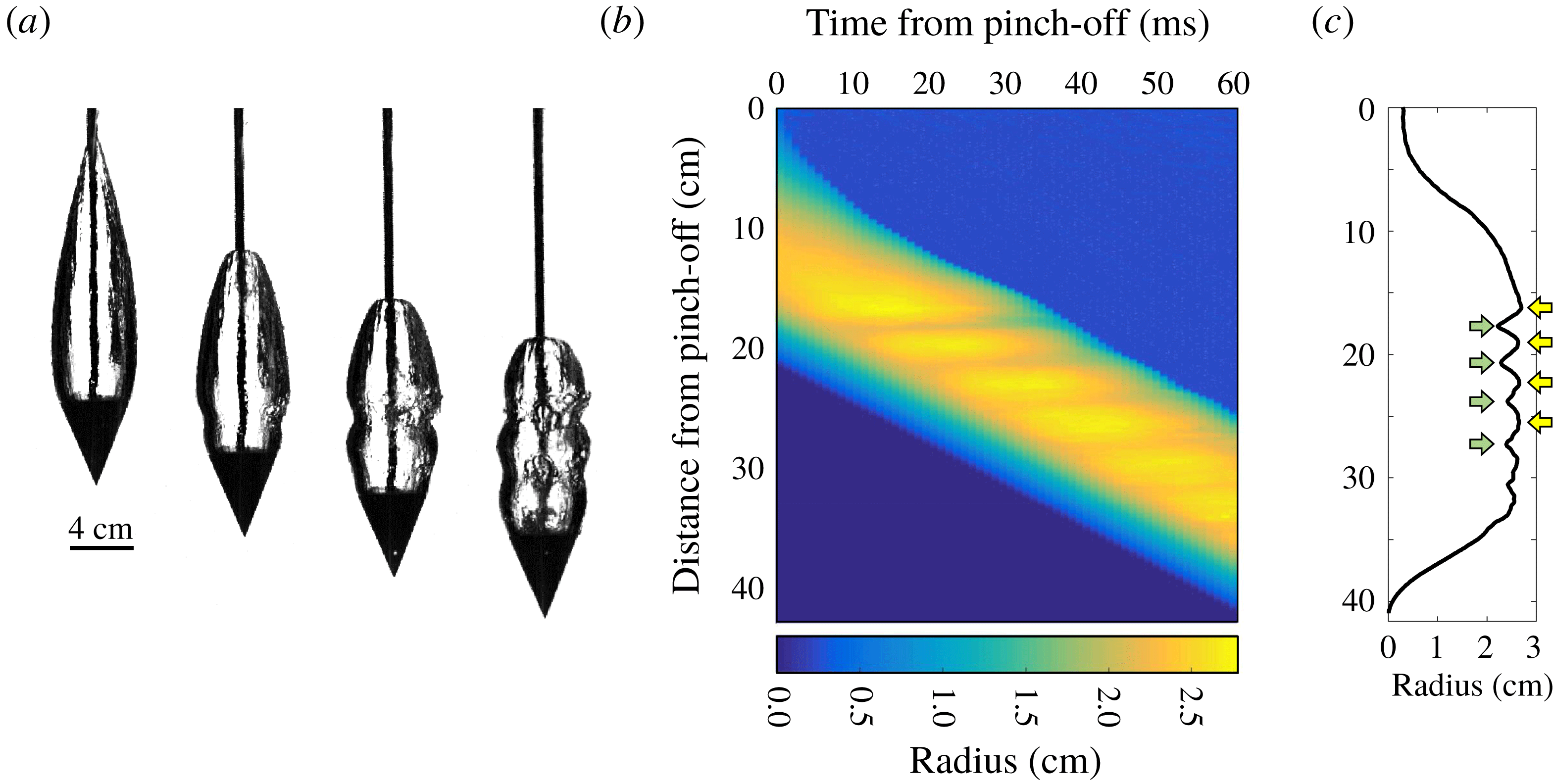
High-speed videos were analysed with a customized MATLAB code to measure the interface profile between the water and the air cavity. First, we zoomed in and cropped an air-cavity shape beyond the cone as shown in figure 3(a). Then, the cone and the rod are recognized and removed from the images and the cavity itself is identified and cropped to apply the image processing algorithm and determine the cavity boundary. Figure 3(b) shows the spatio-temporal plot of the ripples. The colour represents the air-cavity width (yellow for a wide cavity and blue for a narrow cavity). These ripples are observed to be fixed in the laboratory frame while the cone was descending further down. The maximal width over the course of the experiment at a given vertical location is plotted in figure 3(c), which shows a clear sinusoidal profile along the vertical direction.
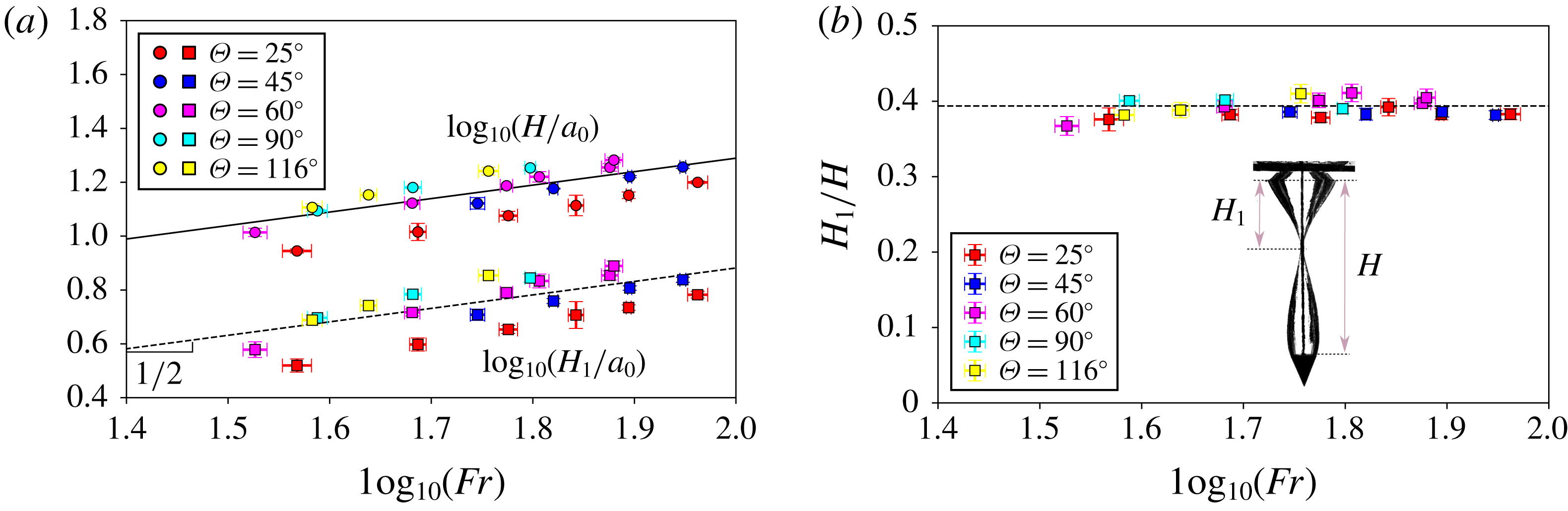
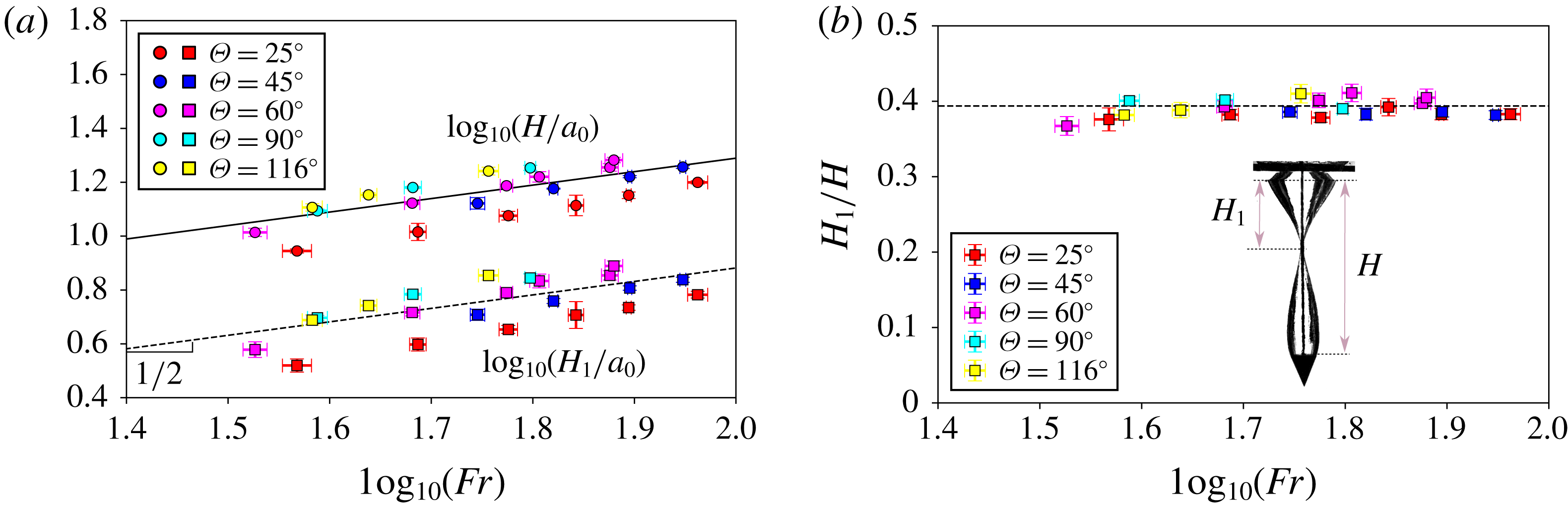
For both plots, each point is an average on 5 measures. (a) Two sets of data are shown concerning either the ratio of cone depth at pinch-off time (
 $H$
) or pinch-off depth (
 $H_{1}$
) to the cone radius (
 $a_{0}$
). The top set shows the logarithmic plot of
 $H/a_{0}$
versus the Froude number, whereas the bottom set shows the logarithmic plot of
 $H_{1}/a_{0}$
versus the Froude number. The dashed line has a prefactor
 $C_{1}=0.8$
with a
 $R^{2}$
of
 $0.5$
and the solid line
 $C_{2}=1.9$
with a
 $R^{2}$
of 0.6. (b) Ratio of the depth of the air cavity and the depth where pinch-off occurs as a function of the logarithm of the Froude number. The experimental value
 $0.39\pm 0.01$
(dashed line) is close to the range 0.39–0.43 obtained on spheres from Mansoor et al. (Reference Mansoor, Marston, Vakarelski and Thoroddsen2014). The inset shows a picture of the cone–air cavity at pinch-off, defining
 $H$
and
 $H_{1}$
.
3.3 Pinch-off depth and air-cavity ripples
We first characterize the pinch-off depth
 $H_{1}$
and the air-cavity depth
 $H$
at the moment of pinch-off. Figure 4(a) shows both the air-cavity and pinch-off depths normalized by the cone radius. Both the air-cavity and pinch-off depths depend on the Froude number as
 $H_{1}/a_{0}=C_{1}Fr^{1/2}$
(dashed line) and
 $H/a_{0}=C_{2}Fr^{1/2}$
(solid line), with the fit coefficients
 $C_{1}=0.8$
and
 $C_{2}=1.9$
for cones. Both coefficients,
 $C_{1}$
and
 $C_{2}$
, are very close to the coefficients obtained for disks of similar radius (10–40 mm) in Bergmann et al. (Reference Bergmann, Van Der Meer, Gekle, Van Der Bos and Lohse2009), where they predict
 $C_{2}=2.2$
and find experimentally
 $C_{2}=2.5$
, with
 $C_{1}$
being calculated as
 $C_{2}/2$
. This
 $Fr^{1/2}$
-dependence of the depths is also reported in other earlier studies with spheres and disks (Glasheen & McMahon Reference Glasheen and McMahon1996; Gaudet Reference Gaudet1998; Duclaux et al.
Reference Duclaux, Caillé, Duez, Ybert, Bocquet and Clanet2007; Bergmann et al.
Reference Bergmann, Van Der Meer, Gekle, Van Der Bos and Lohse2009; Mansoor et al.
Reference Mansoor, Marston, Vakarelski and Thoroddsen2014). Regardless of the cone angle, the pinch-off depth is always located at a depth
 $H_{1}/H\approx 0.39$
(figure 4
b). For spheres Duclaux et al. (Reference Duclaux, Caillé, Duez, Ybert, Bocquet and Clanet2007) predicted a ratio of 0.5 and experimentally found 0.45, while Mansoor et al. (Reference Mansoor, Marston, Vakarelski and Thoroddsen2014) found a ratio between 0.39 and 0.43 for spheres, with the surface sealing up after pinch-off.
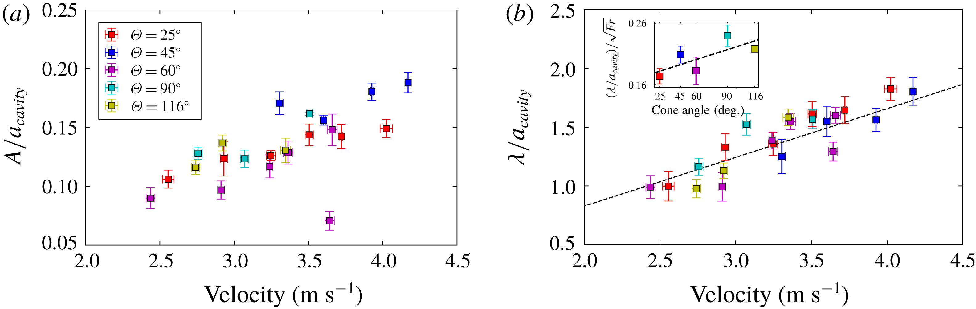
Amplitude and wavelength of the air cavity normalized by the air-cavity radius, for five different cone angles, as a function of the cone velocity. (a) To calculate the amplitude of the cavity, we subtract each temporal profile during descent from the averaged profile. Then we consider the maximum difference of these two profiles normalized with the cone radius as the cavity ripples amplitude velocity. (b) Wavelength between the two first ripples. The black line represents the theoretical value of the linear coefficient 0.415. We have also analysed the characteristics of the following ripples to quantify the wavelength and amplitude variations with respect to distance from the cone. When present, we observed that the decay rate and wavelength of the following ripples do not vary significantly with respect to the first one and are also in agreement with our theoretical predictions. The inset shows the normalized wavelength divided by the square root of the Froude number as a function of the cone angle. A linear trend is observed.
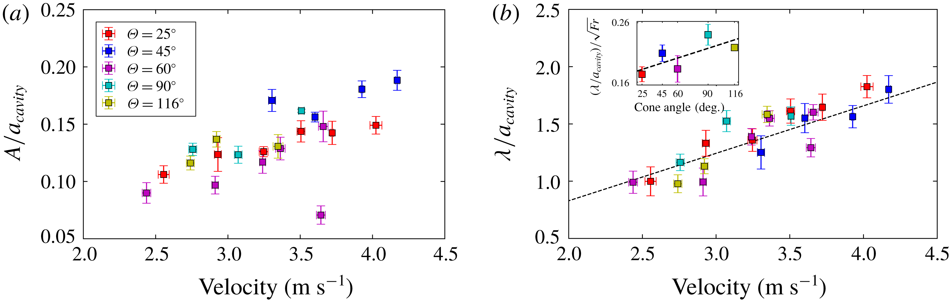
In our experiments, the amplitude and wavelength of the ripples linearly increase as a function of the impact velocity, as shown in figures 5(a) and 5(b), respectively. While our theory uses the cone radius as
 $a_{0}$
to normalize the wavelength and amplitude of the ripples, we use the average maximum radius of the air cavity (similar to Grumstrup et al.
Reference Grumstrup, Keller and Belmonte2007). The average maximum radius for all trials of the air cavity is
 $a_{cavity}\approx 2.56\pm 0.33$
cm. The observed normalized wavelength is found to be in good agreement with the theoretical model (see (2.11)), in which
 $\unicode[STIX]{x1D706}/a_{cavity}\approx 0.415V_{0}$
, with
 $R^{2}=0.75$
. In figure 5(b), we also noticed a small dependence on cone angle for the wavelength–velocity relation in terms of the slope, which we will define as
 $\unicode[STIX]{x1D706}/(a_{cavity}V_{0})$
. For example, the slope for a cone angle of
 $\unicode[STIX]{x1D703}=116^{\circ }$
appears higher than the slope for a cone angle of
 $\unicode[STIX]{x1D703}=25^{\circ }$
. To check this angle dependence, the slope is redefined as
 $N=\unicode[STIX]{x1D706}/(a_{cavity}\,\sqrt[]{Fr})$
, which is shown in the inset of figure 5(b). Here, there appears to be a linear increase in the slope,
 $N$
, with respect to the cone angle,
 $\unicode[STIX]{x1D703}$
. The variation of
 $N$
is only approximately 40 % of its averaged value, which cannot be captured in our current model. However, our model predicts the averaged slope of the wavelength versus velocity as
 $\unicode[STIX]{x1D706}/a_{cavity}\approx 0.415V_{0}$
.
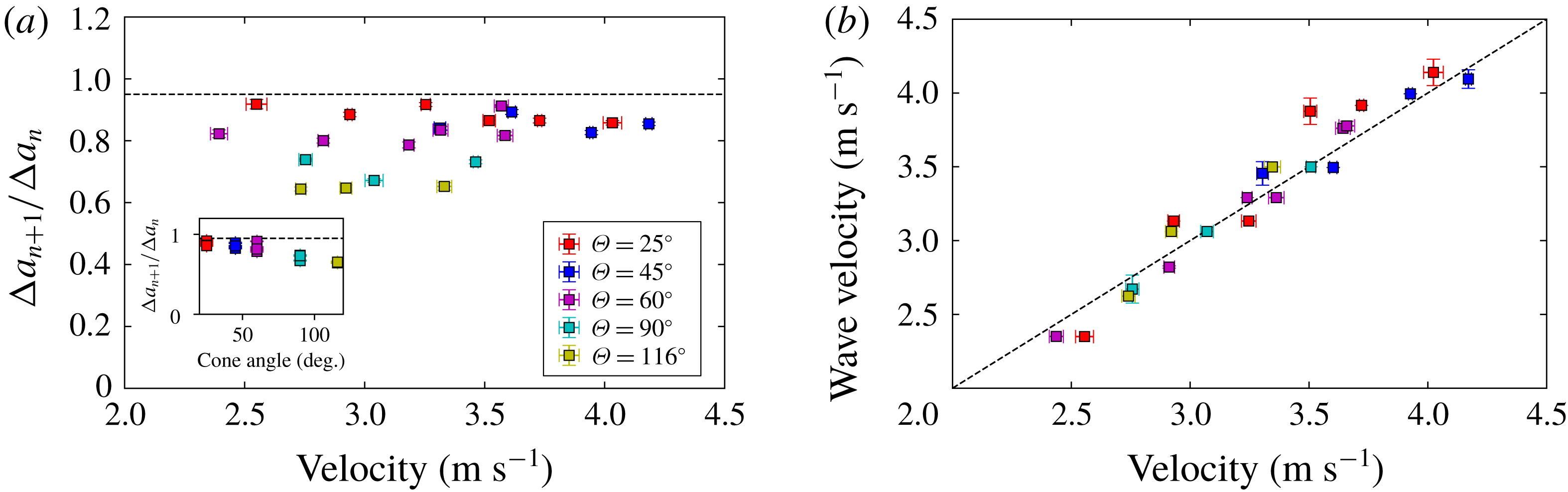
The decay of the amplitude of the ripples with distance from the cone was observed. This decay rate is measured by the ratio of the second and first ripple amplitudes, or
 $\unicode[STIX]{x0394}a_{n+1}/\unicode[STIX]{x0394}a_{n}$
. From (2.10) and (2.11), the decay rate is calculated as
 $\exp (-2\unicode[STIX]{x03C0}\unicode[STIX]{x1D714}_{r}/\unicode[STIX]{x1D714}_{i})\approx 0.95$
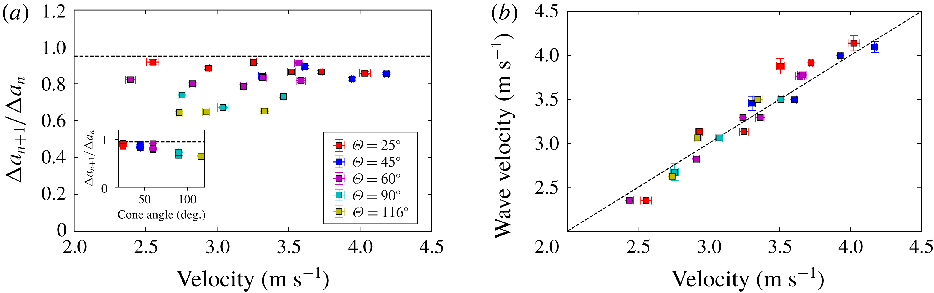
. The experimental decay rates are slightly smaller than this predicted value, as shown in figure 6(a). It is worth noting that a weak dependence between this decay rate and the cone angle is observed, as shown in the inset of figure 6(a).
In our theoretical model, we assumed that the velocity of the air cavity is the same as the projectile velocity. To further validate this assumption, we measured the wave propagation velocity (
 $=\unicode[STIX]{x1D706}f$
), i.e. the velocity of the cavity profile during descent as shown in figure 6(b). A strong linear correlation between the cone and the cavity velocities indicates that the ripples will remain in the laboratory frame rather than following the cone.
(a) Ratio of the first two ripple amplitudes as a function of the cone velocity. The dashed line represents the theoretical damping rate value of 0.95. The inset shows a weak dependence between that same ratio and the cone angle. (b) The wave propagation velocity, i.e. the wave velocity of the cavity with respect to the cone, as a function of the cone velocity for five different cone angles. To calculate the wave velocity, the spatial cavity profiles are averaged and the difference of each profile with averaged profile are obtained. The subsequent profiles are correlated to find the displacement and consequently the cavity profile velocity. The dashed line is the best linear fit, with a slope of 1.01.
3.4 Force data
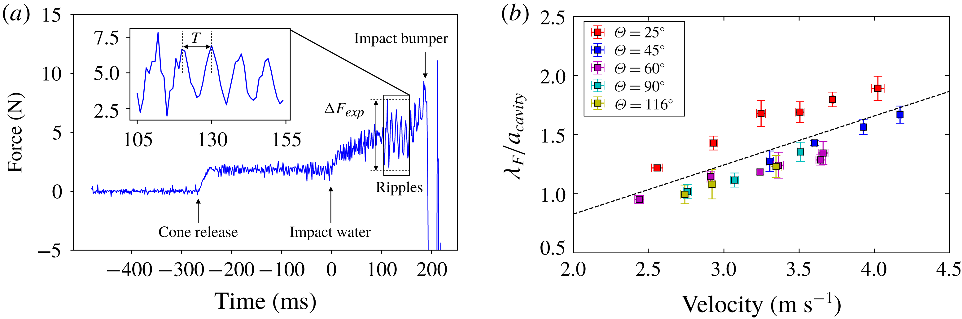
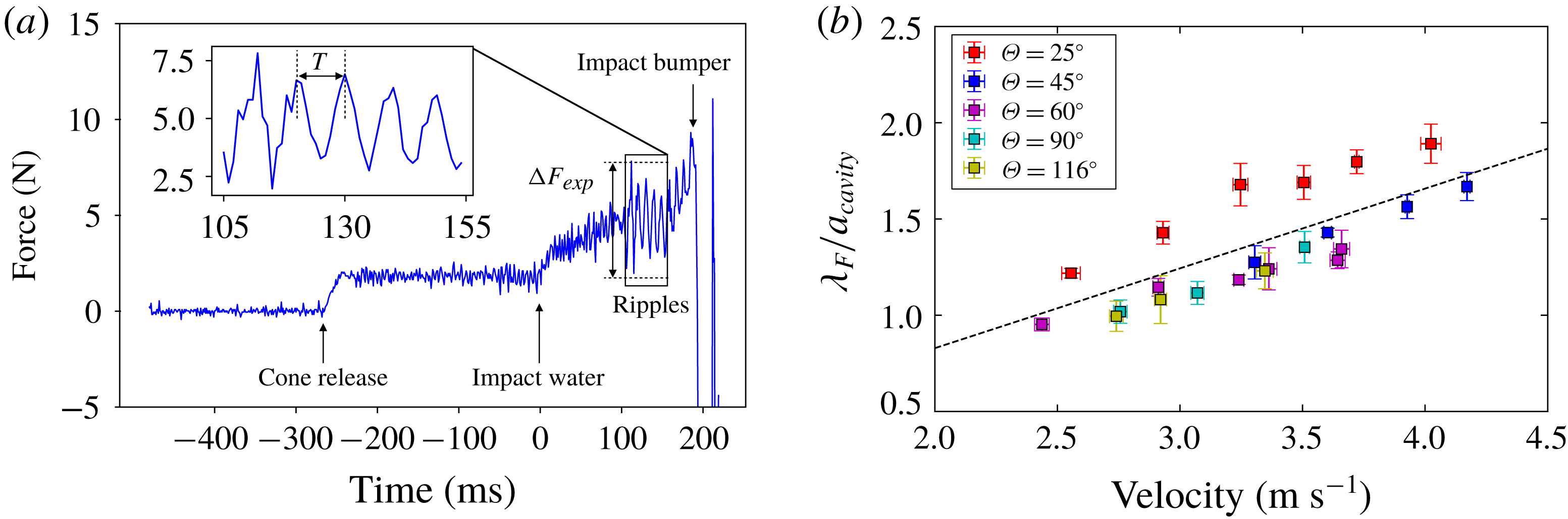
The force profile during water entry is shown in figure 7(a). Upon cone impact, the cone feels a drag force which is proportional to the added mass. Shortly after, as the cone continues to penetrate through the interface, the air cavity forms, which causes a linear increase in force due to a hydrostatic pressure force (Chang et al. Reference Chang, Croson, Straker, Gart, Dove, Gerwin and Jung2016). Upon pinch-off, oscillations in the force profile become visible, presumably from the ripples. At later times past the rippling stage, one may notice an increase in mean force. There are two possible effects causing this. First, the linearly increasing force could be the effect of the hydrostatic pressure force from the atmospheric pressure in the air cavity as the cone travels deeper underwater. The second possible cause is the geometry of the air cavity. Previous literature (Knapp, Daily & Hammitt Reference Knapp, Daily and Hammitt1970; Vincent et al. Reference Vincent, Xiao, Yohann, Jung and Kanso2018) has shown that a longer air cavity behind a body will reduce the drag acting on the body. As the air cavity breaks up and becomes smaller, the drag acting on the cone should increase, which could explain the increasing force at much later times past pinch-off.
In the inset of figure 7(a), we assume that the force variation results from the acoustic wave caused by the air cavity following pinch-off. Similarly to the air-cavity radius, following pinch-off we observe the formation of ripples in the force signal. These force ripples can be characterized by their amplitude and wavelength. The amplitude provides the experimentally measured force variation applied by the air cavity to the cone. Analysis of the force measurement signal showed increased noise and damping towards the end of the time series. On average, the values of the last peak were less than 30 % of the average of the initial peaks. Due to a low signal-to-noise ratio, we eliminate the last peak from the analysis. The average force signal during ripple formation was subtracted from the original signal and by applying power spectrum analysis, the dominant frequency of the signal was obtained, then inversed to obtain the period of the ripples,
 $T$
(inset of figure 7
a). The wavelength was calculated by multiplying the cone velocity by the period
 $T$
.
We can see in figure 7(b) that this wavelength varies linearly with the velocity, with a linear coefficient of 0.407, very close to the predicted 0.415 from theory, and in very good agreement with the wavelength from the air cavity (figure 8 b). This validates that our force measurements come from the ripples.
(a) Typical force pattern observed for a cone angle of
 $45^{\circ }$
and a drop height of 30 cm. The force variation is measured by subtracting the peak and the valley values of the signal. (b) Wavelength between the two first ripples normalized by the radius of the cone as a function of the impact velocity for five different cone angles. The black line represents the theoretical value of the linear coefficient of 0.415 which is very close to the fitted coefficient of 0.407.
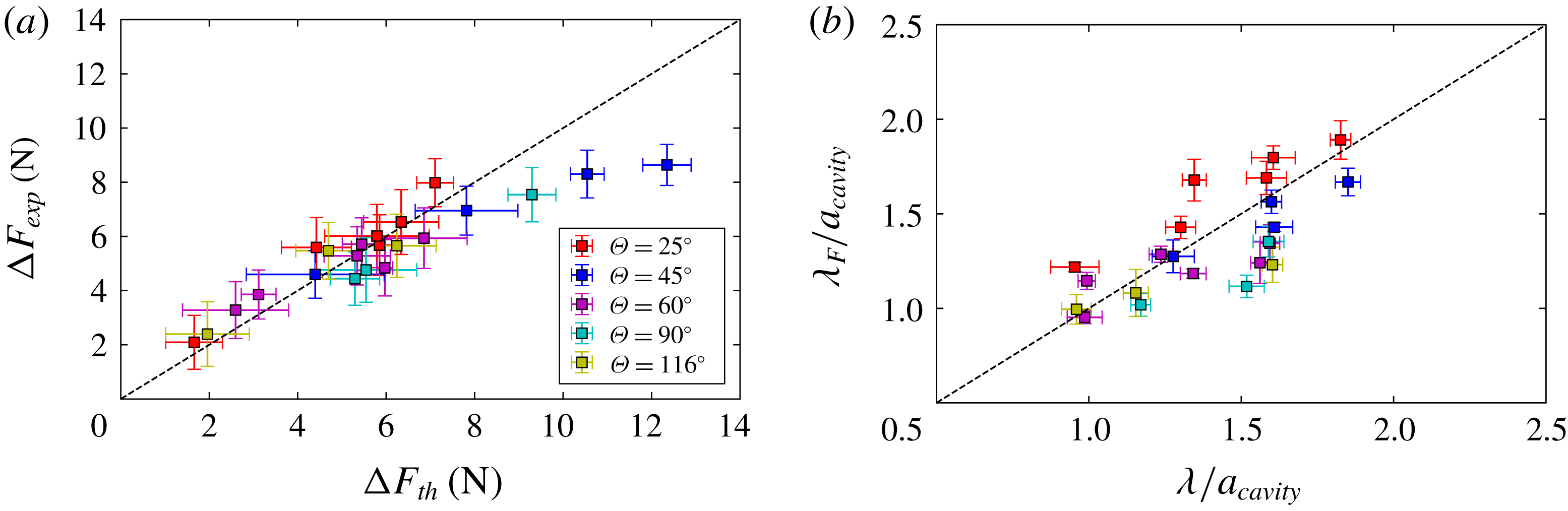
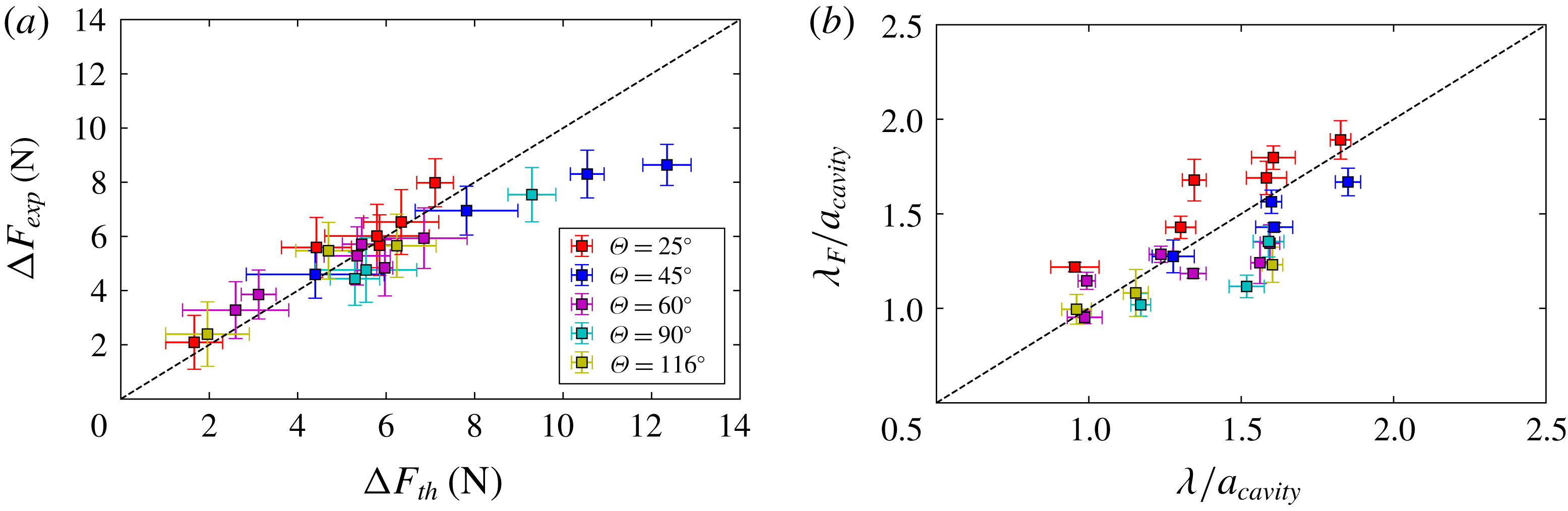
(a) Force measured experimentally using a force sensor, as a function of the estimated force resulting from the measured ripples amplitudes, as in figure 3(c) and using the formula of (3.1). The slope of the dashed line is the theoretical coefficient 1, close to the fitting coefficient 0.9 with a
 $R^{2}$
of 0.7. (b) Wavelength of force signal for five different cone angles, as a function of the wavelength resulting from the ripple measurements, as in figure 5(b). The slope of the dashed line is the theoretical coefficient 1, close to the fitted coefficient of 0.93.
The theoretical force,
 $\unicode[STIX]{x0394}F_{th}$
, is estimated using (2.5). If we assume the flow and pressure fields in the liquid around the cone are the same regardless of the cavity ripples, the only source generating the force fluctuation is the pressure variation due to the ripples in the air cavity. We can then calculate the average pressure in the air cavity, and screen for its maximal and minimal value in a window of length
 $L_{r}$
, the length of the ripples, along the vertical axis. Then, we can write the force amplitude
 $\unicode[STIX]{x0394}F_{th}$
as
 $$\begin{eqnarray}\displaystyle \unicode[STIX]{x0394}F_{th}=\unicode[STIX]{x03C0}R^{2}(\bar{P}_{max}-\bar{P}_{min}). & & \displaystyle\end{eqnarray}$$
The experimental force (
 $\unicode[STIX]{x0394}F_{exp}=F_{max}-F_{min}$
) is compared to the theoretical force
 $\unicode[STIX]{x0394}F_{th}$
in figure 8(a). The relationship between the estimated and measured force amplitudes is
 $\unicode[STIX]{x0394}F_{exp}=0.9\unicode[STIX]{x0394}F_{th}$
. We observe a close in-phase relationship between the force acting on the projectile and the predicted force calculated from the pressure within the air cavity. To investigate the origin of the error bar in our predicted force, an uncertainty analysis has been done on (3.1) and all the uncertainties of the measurements taken into account. The uncertainty of theoretical force difference equation can be calculated by
 $$\begin{eqnarray}\displaystyle U_{\unicode[STIX]{x0394}F_{th}}^{2}=2\left(\left(\frac{\unicode[STIX]{x2202}\unicode[STIX]{x0394}F_{th}}{\unicode[STIX]{x2202}L_{r}}\right)^{2}U_{L_{r}}^{2}+\left(\frac{\unicode[STIX]{x2202}\unicode[STIX]{x0394}F_{th}}{\unicode[STIX]{x2202}V_{0}}\right)^{2}U_{V_{0}}^{2}\right), & & \displaystyle\end{eqnarray}$$
where
 $U_{L_{r}}$
and
 $U_{V_{0}}$
are the uncertainties of respectively the length of the air cavity behind the cone, and the velocity of the cone. By substituting all the terms with their expression, we can rewrite the above equation and estimate an uncertainty on the estimated forces of 1.6 N.
4 Discussion
In this paper, we investigated the dynamics of an air cavity that remains attached to a cone after pinch-off. It was experimentally confirmed that, regardless of the cone angle, the pinch-off is always located at a depth of
 $H_{1}/H\approx 0.39$
, which stands in between theoretical values of
 $1/3$
for cylinders and
 $1/2$
for spheres predicted by Duclaux et al. (Reference Duclaux, Caillé, Duez, Ybert, Bocquet and Clanet2007). After pinch-off, we observed the formation of ripples along the air cavity, which remain fixed in the laboratory frame. The wavelength and amplitude of the ripples increase with the velocity. The relation between the wavelength and velocity is predicted from an acoustic model (proposed by Grumstrup et al.
Reference Grumstrup, Keller and Belmonte2007) as
 $\unicode[STIX]{x1D706}/a_{cavity}\approx 0.415V_{0}$
(Grumstrup et al.
Reference Grumstrup, Keller and Belmonte2007). Our experiments are in good agreement with the theoretical prediction. The velocity dependence on the amplitude is due to the pressure wave from pinch-off and decays due to acoustic radiation, which our linear stability analysis cannot predict. However, the theoretical damping rate of the amplitude can be predicted, but is a 10 % overestimation of the experimental observations, which indicates another possible damping source, such as viscous damping. Our theoretical model can capture the general physics of the rippling behaviour by taking into account the average maximal cavity radius. However, there appears to be a small dependence between the cone angle and the maximum air-cavity radius.
Lastly, the measured force and associated wavelengths from the force sensor are found to be linearly proportional, with a best fit coefficient close to one, to the estimated force from the ripple’s amplitude and wavelength, respectively. This suggests a close in-phase relationship between the fluctuation in the force acting on the projectile and the ripples on the air cavity. It is worth noting that data obtained from the force sensor also show a better accuracy both in terms of reproducibility and agreement with the theory than data obtained with the high-speed camera.
Even though we have focused on the dynamics of the air cavity following a cone after pinch-off in this paper, our approach can be extended to other projectiles with various geometries as long as the air cavity has a fixed contact line on the projectile. For future work, we will use a soft projectile body or a rigid projectile with a soft outer surface similar to bird feathers. Very recently, studies conducted on diving sea birds have investigated the fluids forces acting on the bird’s neck when diving (Chang et al. Reference Chang, Croson, Straker, Gart, Dove, Gerwin and Jung2016). By extending their approach to our study, we can design a cone with feathers that could give rise to a fluid–structure interaction between the air cavity and the elastic body, enhancing or inhibiting the ripples and the corresponding emitted sounds. An additional study to enhance or inhibit the ripples is to study the effects of surface wettability.
Acknowledgement
This work was supported by the NSF under CBET-1336038 and CBET-1604424.
Appendix A.
In this appendix, we follow the work described in Epstein & Keller (Reference Epstein and Keller1972) for linearizing the Bernoulli equation, starting with
 $$\begin{eqnarray}\displaystyle P(r,t)=P_{0}-\unicode[STIX]{x1D70C}\left(\unicode[STIX]{x1D6F7}_{t}+{\textstyle \frac{1}{2}}\unicode[STIX]{x1D6F7}_{r}^{2}\right). & & \displaystyle\end{eqnarray}$$
At the interface with small-amplitude ripples, the radius is expressed as
 $r=a_{0}+a(t)$
, where
 $a_{0}$
is the initial radius of the cavity. With the small-amplitude ripples, the left-hand side of the Bernoulli equation may be linearized as
 $P(a_{0}+a(t),t)=P(a_{0})+a(t)P_{r}|_{r=a_{0}}$
, resulting in
 $$\begin{eqnarray}\displaystyle P(a_{0})+a(t)P_{r}|_{r=a_{0}}=P_{0}-\unicode[STIX]{x1D70C}\left(\unicode[STIX]{x1D6F7}_{t}+{\textstyle \frac{1}{2}}\unicode[STIX]{x1D6F7}_{r}^{2}\right). & & \displaystyle\end{eqnarray}$$
Dropping the higher-order term on the right-hand side and defining
 $P_{0}=P(a_{0})$
would result in the linearized Bernoulli equation as seen in (2.3):
 $$\begin{eqnarray}\displaystyle P_{r}|_{r=a_{0}}\,a(t)=-\unicode[STIX]{x1D70C}\,\unicode[STIX]{x1D6F7}_{t}. & & \displaystyle\end{eqnarray}$$
Appendix B.
In this appendix, we carry out the derivation of the dispersion relation between (2.8) and (2.9). Starting with (2.8), the dispersion relation looks like
 $$\begin{eqnarray}\displaystyle \unicode[STIX]{x1D714}^{2}\text{K}_{0}(x)=\frac{\unicode[STIX]{x1D714}}{\unicode[STIX]{x1D70C}c}P_{r}|_{r=a_{0}}\,\text{K}_{1}(x), & & \displaystyle\end{eqnarray}$$
where
 $x=\unicode[STIX]{x1D714}a_{0}/c$
. In the limit of large
 $\unicode[STIX]{x1D714}$
, an asymptotic expansion of the modified Bessel function of the second kind takes the form
 $\text{K}_{0}(x)=(\unicode[STIX]{x03C0}/2x)^{1/2}\text{e}^{-x}(1-1/8x+\cdots \,)$
and
 $\text{K}_{1}(x)=-\unicode[STIX]{x2202}\text{K}_{0}(x)/\unicode[STIX]{x2202}x=(\unicode[STIX]{x03C0}/2x)^{1/2}\text{e}^{-x}(1+3/8x+\cdots \,)$
, which results in
 $$\begin{eqnarray}\displaystyle & \displaystyle \unicode[STIX]{x1D714}^{2}\left(1-\frac{1}{8x}\right)=\frac{\unicode[STIX]{x1D714}}{\unicode[STIX]{x1D70C}c}P_{r}|_{r=a_{0}}\left(1+\frac{3}{8x}\right), & \displaystyle\end{eqnarray}$$
 $$\begin{eqnarray}\displaystyle & \displaystyle \unicode[STIX]{x1D714}^{2}=\frac{\unicode[STIX]{x1D714}}{\unicode[STIX]{x1D70C}c}P_{r}|_{r=a_{0}}\left(1+\frac{3}{8x}\right)\left(\frac{1}{1-\displaystyle \frac{1}{8x}}\right). & \displaystyle\end{eqnarray}$$
Noting that
 $1/(1-(1/x))=1+(1/x)$
through a series expansion at
 $x=\infty$
, or a Laurent series, the equation from above gives
 $$\begin{eqnarray}\displaystyle \unicode[STIX]{x1D714}^{2}=\frac{\unicode[STIX]{x1D714}}{\unicode[STIX]{x1D70C}c}P_{r}|_{r=a_{0}}\left(1+\frac{3}{8x}\right)\left(1+\frac{1}{8x}\right). & & \displaystyle\end{eqnarray}$$
Further simplification leads to
 $$\begin{eqnarray}\displaystyle \unicode[STIX]{x1D714}^{2}=\frac{\unicode[STIX]{x1D714}}{\unicode[STIX]{x1D70C}c}P_{r}|_{r=a_{0}}\left(1+\frac{1}{2x}+\frac{3}{64x}\right). & & \displaystyle\end{eqnarray}$$
Finally, dropping the high-order term and saying
 $x=\unicode[STIX]{x1D714}a_{0}/c$
, we get the dispersion relation for large
 $\unicode[STIX]{x1D714}$
seen in (2.9):
 $$\begin{eqnarray}\displaystyle \unicode[STIX]{x1D714}^{2}=\frac{\unicode[STIX]{x1D714}}{\unicode[STIX]{x1D70C}c}P_{r}|_{r=a_{0}}\left(1+\frac{c}{2\unicode[STIX]{x1D714}a_{0}}\right). & & \displaystyle\end{eqnarray}$$