





1. Introduction
The behaviour of liquids in contact with solid surfaces is strongly influenced by geometry, and can become significantly more complex in the presence of curvature, edges or confinement. One important example is provided by liquid bridges, which arise when a volume of liquid is deposited into the gap between nearby solid bodies. Understanding such systems is important for a wide range of applications, including granular materials, lubrication, porous media and foams. Such bridges have been studied in a wide range of geometrical configurations, including between planar, spherical and cylindrical surfaces. A number of classical works have provided detailed descriptions of equilibrium capillary-bridge shapes using analytical and semi-analytical approaches based on the Young–Laplace (YL) equation, particularly in idealised geometries, see e.g. Rose (Reference Rose1958), Cross & Picknett (Reference Cross and Picknett1963), Melrose (Reference Melrose1966), Clark et al. (Reference Clark, Haynes and Mason1968) and Orr et al. (Reference Orr, Scriven and Rivas1975). A general theoretical framework for capillary phenomena, including liquid bridges in various geometries, is provided in the monograph by Myshkis et al. (Reference Myshkis, Babskii, Kopachevskii, Slobozhanin and Tyuptsov1987), with particular emphasis on situations in which gravitational effects are weak or negligible, in contrast to the regime considered in the present study. A substantial body of work has been devoted to understanding the capillary forces exerted by liquid menisci, including liquid bridges – see, for example, the comprehensive review by Butt & Kappl (Reference Butt and Kappl2008).
Later, the effect of gravity on liquid bridges was analysed in more detail, including its influence on equilibrium shapes and their stability, see, for example, Lowry & Steen (Reference Lowry and Steen1995), Laverón-Simavilla & Perales (Reference Laverón-Simavilla and Perales1995) and Adams et al. (Reference Adams, Johnson, Seville and Willett2002). Gravitational effects can typically be neglected when the size of the bridge is small compared with the capillary length, but become important when these length scales are comparable. Although multiple equilibrium solutions may exist, only stable configurations are physically realised, and changes in stability govern transitions between different bridge shapes. The stability of capillary surfaces, including liquid bridges, is reviewed by Bostwick & Steen (Reference Bostwick and Steen2015), and is closely related to the bifurcation structure of solutions examined in our study.
A configuration of primary interest in the present work is that of liquid bridges between two parallel identical horizontal cylinders. This problem was first studied in detail by Princen (Reference Princen1970), who analysed this problem in the absence of gravity and in the limit of sufficiently long bridges, for which the bridge cross-section becomes nearly uniform away from the end menisci. In this regime, adding liquid increases the length of the bridge without significantly affecting its cross-sectional shape, so that a two-dimensional (2-D) approximation applies. Three-dimensional (3-D) extensions to non-parallel cylinders, for example, have also been considered (see e.g. Virozub et al. Reference Virozub, Haimovich and Brandon2009). When gravitational effects are taken into account, a closely related 2-D configuration was analysed by Cooray et al. (Reference Cooray, Huppert and Neufeld2016), who considered steady-state liquid bridges between parallel horizontal cylinders in the presence of gravity. They derived analytical descriptions of the liquid–air interface based on exact solutions of the YL equation involving incomplete elliptic integrals, and obtained approximations in the limits of small and large liquid volumes. They also investigated the maximum trapping capacity between the cylinders, showing that the maximum cross-sectional area is achieved when the separation distance is approximately twice the capillary length.
This motivates the present study, where we investigate how the application of an electric field, in addition to gravity, modifies the behaviour of liquid bridges. In particular, we consider liquid bridges formed between pairs of identical horizontal cylinders, using transformer oils that can be modelled as perfect dielectrics, with the cylinders acting as electrodes between which a potential difference can be applied. Electric fields can significantly affect the behaviour of liquid interfaces through Maxwell stresses. A wide range of such phenomena has been studied, including interfacial deformation, instabilities and electrically driven flows, see, for example, the reviews by Vlahovska (Reference Vlahovska2019) and Papageorgiou (Reference Papageorgiou2019) and the monograph by Castellanos et al. (Reference Castellanos, Zhakin, Watson, Atten and Chang1998). Within this broad area, previous studies of electrified liquid bridges have focused primarily on the axisymmetric configuration of liquid bridges between parallel planar electrodes with pinned three-phase contact lines, analysing mainly equilibrium shapes, their stability and the associated bifurcation structure under axial electric fields, both in the absence and presence of axial gravity, see e.g. Gonzalez et al. (Reference Gonzalez, McCluskey, Castellanos and Barrero1989), Ramos & Castellanos (Reference Ramos and Castellanos1993) and Volkov et al. (Reference Volkov, Papageorgiou and Petropoulos2005) and the review by Montanero & Ponce-Torres (Reference Montanero and Ponce-Torres2020). Extending the analysis to the current set-up of liquid bridges between horizontal cylinders requires addressing several additional challenges because such bridges are inherently non-axisymmetric, the contact lines are free to move over the surfaces of the cylinders and the bridge behaviour is governed by the coupled effects of the curvature of the supporting cylinders, gravity and the non-local electric field.
We begin by considering equilibrium configurations, which constitute the initial focus of the present work. For such states, the flow is absent, and the corresponding liquid–air interfaces are determined from YL-type equations incorporating non-local electric-field contributions, in a manner similar to that employed for axisymmetric electrified liquid bridges (e.g. Ramos & Castellanos Reference Ramos and Castellanos1993; Volkov et al. Reference Volkov, Papageorgiou and Petropoulos2005). To evaluate non-local electric-field contributions, we use a boundary-element method. The time-dependent behaviour of liquid bridges is of independent interest, as it can involve non-trivial evolution and regime transitions, and it has been widely studied, particularly in axisymmetric geometries (see, e.g. Suryo & Basaran Reference Suryo and Basaran2006; Slobozhanin et al. Reference Slobozhanin, Shevtsova, Alexander, Meseguer and Montanero2012; Li & Sprittles Reference Li and Sprittles2016). However, a complete time-dependent electrohydrodynamic formulation for the present configuration requires solving simultaneously for the fluid motion and the electric field, which are coupled through the evolving free surfaces. This leads to a considerably more involved moving-boundary problem, particularly in the presence of moving contact lines on curved solid surfaces, and is beyond the scope of the present study. Nevertheless, the transient dynamics of non-electrified liquid bridges is of considerable interest in its own right and provides a natural first step towards understanding the evolution of liquid bridges between horizontal cylinders. Accordingly, we derive a reduced-order dynamical model for non-electrified liquid bridges between horizontal cylinders using Onsager’s variational principle (see e.g. Doi Reference Doi2013; Lopes et al. Reference Lopes, Thiele and Hazel2017; Wu et al. Reference Wu, Di, Man and Doi2019). To our knowledge, this is the first reduced-order dynamical model for liquid bridges between horizontal cylinders derived within Onsager’s variational framework. We validate its predictions against direct numerical simulations (DNS) performed within the open-source volume-of-fluid (VOF) platform Basilisk (Popinet Reference Popinet2009, Reference Popinet2015).
The rest of the paper is organised as follows. In § 2, we describe the experimental set-up, and in § 3 the governing equations. Section 4 presents steady-state solutions, including their mathematical formulation, computation and comparison with experiments. Section 5 studies the dynamics of liquid bridges in the absence of an electric field, including the derivation of a reduced-order Onsager model, analysis of its predicted dynamics and comparison with DNS. Details of our DNS implementation within the Basilisk platform are provided in Appendix A. Finally, § 6 presents the conclusions.
2. Experiments
To study liquid bridges suspended between two horizontal cylinders under an applied electric field, we designed a customised experimental set-up (see figure 1). Two parallel cylindrical electrodes with a
 $2$
mm diameter are held by an adjustable plastic rig, where the separation distance can be varied (figure 1
b). The electrodes are connected to a high-voltage DC power source (model PS/FJ30R04.0-22, FJ Glassman High Voltage Inc.), allowing the application of potentials of up to
 $4000$
V, and the system is enclosed in a transparent box with a safety interlock (figure 1
a). A digital multimeter (Philips PM 2522A VAΩ) is used to measure potential difference. The electrodes can be replaced, in order to vary properties such as the contact angle with the liquid, and were made of platinised titanium, copper and stainless steel rods.
Parameters of the transformer oils used in the experiments.

Table 1. Long description
A table comparing parameters of different transformer oils. The table has 6 rows and 5 columns. The columns are labeled Parameter, Unit, Mineral oil, Castor oil, Silicone oil 5 cSt, and Silicone oil 500 cSt. The rows list parameters such as density, surface tension, kinematics viscosity, Bond number, contact angle with stainless steel, and contact angle with copper. Each row provides specific values for each type of oil. For example, the density of Mineral oil is 833 kg/m^3, Castor oil is 961 kg/m^3, Silicone oil 5 cSt is 913 kg/m^3, and Silicone oil 500 cSt is 970 kg/m^3. The surface tension values are 0.028 N/m for Mineral oil, 0.039 N/m for Castor oil, 0.02 N/m for Silicone oil 5 cSt, and 0.0212 N/m for Silicone oil 500 cSt.
Schematic diagram of (a) the safety box, including (b) the experimental rig, DC power supply, digital multimeter, top and front view cameras.

Front view of silicone-oil bridge suspended between platinised titanium rods, for (a) non-electrified case, (b)
 $2000\, \mathrm{V}$
and (c)
 $3000\, \mathrm{V}$
. Top view of silicone-oil bridge suspended between platinised titanium rods corresponding to (d) non-electrified case, (e)
 $2000\, \mathrm{V}$
and (f)
 $3000\, \mathrm{V}$
. The movies for these are available as supplementary material at https://doi.org/10.1017/jfm.2026.12035.

Experiments were performed using pure non-conducting oils, namely mineral, castor and silicon oils. In table 1, we present a summary of the relevant material properties of the oils. Note that the contact angles were measured using a drop shape analyser (DSA100E, KRÜSS Scientific), and the values reported in table 1 correspond to clean flat surfaces. However, we also observed significant variations due to surface roughness, and, therefore, these angles should be viewed as indicative and with a precision of around
 $\pm 5^\circ$
. Both electrified and non-electrified liquid bridges were recorded using front and top view cameras.
Front view of castor oil suspended between copper rods corresponding to (a) non-electrified case, (b)
 $2000\, \mathrm{V}$
, (c)
 $3000\, \mathrm{V}$
and (d)
 $4000\, \mathrm{V}$
. The movie for this is available as supplementary material.

Top view of castor oil suspended between copper rods corresponding to (a) non-electrified case, (b)
 $2000\, \mathrm{V}$
, (c)
 $3000\, \mathrm{V}$
and (d)
 $4000\, \mathrm{V}$
. The movie for this is available as supplementary material.

Before each experiment, the electrodes were cleaned with acetone, then distilled water and dried using compressed air. A liquid bridge was formed by depositing an oil droplet of volume
 $\mathtt {\approx } 20 \, {\unicode[Arial]{x03BC}} \mathrm{l}$
between the electrodes using a pipette (RS PRO Pipette PE
 $5$
ml). The bridge was in contact with the electrodes and surrounded by air, without contacting the supporting plate, as shown in figure 2(a–c). After the settling of the bridge, video recording was started at zero applied voltage, followed by gradual increase of the voltage difference up to
 $4 000\, \mathrm{V}$
, over a period of
 $5$
s. During the following
 $5$
seconds the maximum voltage was held. Finally, the voltage difference was reduced gradually to zero over a further period of
 $5$
seconds, and then, after a few more seconds, the recording was ended.
We observed similar behaviour for the three oils. Representative results for silicone oil are shown in figure 2 and for castor oil in figures 3 and 4. In the absence of an electric field, the liquid bridge quickly settles into an equilibrium shape, which hangs low due to the gravitational pull on the liquid. Since the capillary length of the liquid bridge is smaller than the separation between the electrodes, gravitational effects cannot be neglected. The front and top views of the initial non-electrified state are shown for the silicone-oil bridge in figures 2(a) and 2(d) and for the castor-oil bridge in figures 3(a) and 4(a).
When an electric field is applied, the bridge moves upwards and the liquid–air interfaces become noticeably flatter. At the same time, the bridge extends along the electrodes (as seen in the top views), causing the reduction in the cross-sectional area. At higher voltages, the bridge reaches the maximal length and the minimal cross-sectional area (see figures 2 c and 4 d, for silicone and castor oils, respectively). One can also observe that oils with higher viscosity react slower to the electric field changes, as expected.
These observations can be understood by noting that the applied electric field induces stresses at the liquid–air interfaces. These stresses compete with gravity and surface tension, leading to a new equilibrium shape, in which the liquid is drawn into the region between the electrodes, where the electric field is strongest.
3. Full governing equations
Schematic of the two-dimensional model geometry for an electrified pendant liquid bridge between two identical parallel cylinders of cross-sectional radius
 $r$
, with the distance
 $2d$
between the surfaces of the cylinders. The cylinders are electrodes with potential difference
 $V$
applied between them. The electric potential is denoted by
 $\varphi _l$
in the liquid and by
 $\varphi _g$
in the air. The equilibrium three-phase contact angle is
 $\theta _0$
and angles
 $\alpha _1$
,
 $\alpha _2$
specify the locations of the three-phase contact lines. Here,
 $\varSigma _1$
and
 $\varSigma _2$
denote the upper and lower liquid–air interfaces, respectively.

To describe the experiments via a mathematical model, we account for the following physical effects beyond electrostatics and gravity: capillarity (equilibrium contact angle and surface tension), fluid flow and viscosity. We consider a liquid bridge between two parallel horizontal cylinders with cross-sectional radius
 $r$
. The distance between the surfaces of the cylinders is
 $2d$
. The cylinders are electrodes and there is potential difference
 $V$
applied between them. The liquid is assumed to be a dielectric with permittivity
 $\epsilon _l$
(certainly true for the transformer oils used in our experiments), and we assume that it has constant density
 $\rho$
and dynamic viscosity
 $\mu$
. The permittivity of air is denoted by
 $\epsilon _g$
. We introduce Cartesian coordinate axes
 $(x,y,z)$
, with the
 $x$
-axis being horizontal and perpendicular to the axes of the cylinders, which lie in the
 $y$
-direction; the
 $y$
-axis is located right between them. The
 $z$
-axis points upwards, so the acceleration due to gravity
 $\boldsymbol{g}$
points in the negative
 $z$
direction. We consider a 2-D formulation, assuming invariance along the cylinder axis (i.e. the
 $y$
-direction). This corresponds to sufficiently long bridges, where the cross-section is approximately uniform (in the regions away from the end menisci), as in the classical analysis of Princen (Reference Princen1970). A schematic representation is shown in figure 5.
We now present the full governing equations, which form the basis for later derivations. The flow in the liquid is governed by the incompressible Navier–Stokes equations
 \begin{equation} \rho \frac {\text{D}\boldsymbol{u}}{\text{D}t} = - \boldsymbol{\nabla }\!p + \mu \boldsymbol{\nabla} ^2 \boldsymbol{u} + \rho \boldsymbol{g}, \end{equation}
 \begin{equation} \boldsymbol{\nabla }\boldsymbol{\cdot }\boldsymbol{u} = 0, \end{equation}
where
 $\boldsymbol{u}=(u,w)$
and
 $p$
are the velocity and the pressure in the liquid, respectively, and
 $\text{D}/\text{D}t$
denotes the material derivative. Without loss of generality, it can be assumed that the pressure in the air is zero. Note that for perfect dielectric liquids of constant permittivity there is no electric-field contribution in the Navier–Stokes equations, and the coupling between the hydrodynamics and electrostatic phenomena takes place at the liquid–air interfaces, as explained below.
On the parts of the cylinder in contact with the liquid, we assume Navier slip conditions to allow for the motions of the contact lines, and we denote the equilibrium contact angle that the liquid makes with the cylinder surface by
 $\theta _0$
.
As usual, we treat the liquid–air interfaces as surfaces of zero thickness. The upper and lower interfaces are denoted by
 $\varSigma _1$
and
 $\varSigma _2$
and are given by the equations
 $f_1(x,z,t)=0$
and
 $f_2(x,z,t)=0$
, respectively. In the simplest case,
 $\varSigma _1$
and
 $\varSigma _2$
are given by the functions
 $z=h_1(x,t)$
and
 $z=h_2(x,t)$
, respectively, and in such a case
 $f_1(x,z,t)=z-h_1(x,t)$
and
 $f_2(x,z,t)=z-h_2(x,t)$
.
At the liquid–air interfaces, we impose the kinematic boundary conditions
 \begin{equation} \frac {\text{D}f_i}{\text{D}t}=0\quad \text{on}\quad \varSigma _i,\quad i=1,2, \end{equation}
and the stress balance conditions
 \begin{equation} \boldsymbol{n}_i \boldsymbol{\cdot }\boldsymbol{T}_{\!l} - \boldsymbol{n}_i \boldsymbol{\cdot }\boldsymbol{T}_{\!g}= \gamma _{lg}\, \kappa _i \, \boldsymbol{n}_i\quad \text{on}\quad \varSigma _i,\quad i=1,2. \end{equation}
Here,
 $\gamma _{lg}$
is the liquid–air surface tension,
 $\boldsymbol{n}_i$
is the unit normal vector to the interface
 $\varSigma _i$
pointing into the liquid and
 $\kappa _i = \boldsymbol{\nabla }\boldsymbol{\cdot }\boldsymbol{n}_i$
is the curvature of
 $\varSigma _i$
,
 $i=1,2$
. Also,
 $\boldsymbol{T}_{\!l}$
and
 $\boldsymbol{T}_{\!g}$
are the stress tensors in the liquid and in the air, respectively, given by
 \begin{equation} \boldsymbol{T}_{\!l}= \boldsymbol{\sigma }_l+ \boldsymbol{\sigma }_l^M, \qquad \boldsymbol{T}_{\!g}= \boldsymbol{\sigma }_g^M, \end{equation}
where
 $\boldsymbol{\sigma }_l=-p \boldsymbol{I} + \mu (\boldsymbol{\nabla }\boldsymbol{u}+\boldsymbol{\nabla }\boldsymbol{u}^T)$
is the Newtonian stress tensor in the liquid,
 $\boldsymbol{I}$
is the identity matrix, and
 $\boldsymbol{\sigma }_l^M$
and
 $\boldsymbol{\sigma }_g^M$
are the Maxwell stress tensors (Saville Reference Saville1997; Castellanos et al. Reference Castellanos, Zhakin, Watson, Atten and Chang1998) in the liquid and in the air, respectively, given by
 \begin{align} \boldsymbol{\sigma }_l^M &= \epsilon _l\, \boldsymbol{E}_{l} \, \boldsymbol{E}_{l}-\frac {1}{2} \, \epsilon _l (\boldsymbol{E}_{l} \boldsymbol{\cdot }\boldsymbol{E}_{l} ) \boldsymbol{I}, \\[-12pt]\nonumber \end{align}
 \begin{align} \boldsymbol{\sigma }_g^M &=\epsilon _g \, \boldsymbol{E}_{g} \, \boldsymbol{E}_{g}-\frac {1}{2}\, \epsilon _g (\boldsymbol{E}_{g} \boldsymbol{\cdot }\boldsymbol{E}_{g}) \boldsymbol{I}. \end{align}
Here,
 $\boldsymbol{E}_{l}=-\boldsymbol{\nabla }\varphi _l$
and
 $\boldsymbol{E}_{g}=-\boldsymbol{\nabla }\varphi _g$
are the electric fields in the liquid and in the air, respectively, with
 $\varphi _l$
and
 $\varphi _g$
denoting the respective electric potentials.
The electric potentials must satisfy Laplace’s equation. Therefore
 \begin{align} \boldsymbol{\nabla} ^2 \varphi _l=0, \qquad \boldsymbol{\nabla} ^2 \varphi _g=0. \end{align}
Without loss of generality, we assume that
 \begin{align} \varphi _l &= -\frac {V}{2}, \quad \, \varphi _g=-\frac {V}{2} \, \quad \text{on the left cylinder}, \\[-12pt]\nonumber \end{align}
 \begin{align} \varphi _l&=\frac {V}{2}, \quad \quad \varphi _g=\frac {V}{2} \quad \quad \text{on the right cylinder}. \end{align}
Also, in the far field
 $ \varphi _g \rightarrow 0$
as
 $(x^2+z^2)\rightarrow \infty$
.
At the liquid–air interfaces the electric potential must be continuous, i.e.
 $\varphi _l=\varphi _g$
, and we must have continuity of the normal component of the electric displacement
 \begin{equation} \boldsymbol{n}_i \boldsymbol{\cdot }\left (\epsilon _l \boldsymbol{\nabla }\varphi _l\right )= \boldsymbol{n}_i \boldsymbol{\cdot }\left (\epsilon _g \boldsymbol{\nabla }\varphi _g\right )\quad \text{on}\quad \varSigma _i,\quad i=1,2. \end{equation}
In the rest of the manuscript, we exploit the symmetry about the
 $z$
-axis. Therefore, it is enough to consider only the domain where
 $x\geqslant 0$
, imposing appropriate symmetry conditions at
 $x=0$
(namely, zero normal velocity, zero normal derivatives of the tangential velocity and pressure, zero electric potential and zero slopes of the top and bottom liquid–air interfaces).
We note that the important dimensionless parameters that determine the equilibrium states of the system are the Bond number (measuring the relative importance of gravitational force to surface tension) and the electric Bond number (measuring the relative importance of electric force to surface tension) given by (see e.g. Berthier & Brakke Reference Berthier and Brakke2012)
 \begin{align} B = \frac {\rho \, g\, r^2}{\gamma _{lg}}, \qquad B_e = \frac {\epsilon _l V^2}{r \, \gamma _{lg}}, \end{align}
respectively, as well as the permittivity ratio,
 $\tilde {\epsilon }_l=\epsilon _l/\epsilon _g$
, the dimensionless half-distance between the cylinders,
 $\tilde {d}=d/r$
, and the equilibrium three-phase contact angle,
 $\theta _0$
.
For the dynamics, another important dimensionless parameter is the Reynolds number,
 $Re={\rho \, U\, r}/{\mu }$
, measuring the relative importance of inertia to viscosity, where
 $U$
is a characteristic velocity scale. However, for the reduced-order model derived later, we restrict attention to the overdamped regime in which inertia is negligible.
4. Steady-state solutions
In the static case, we find that the shapes of the interfaces
 $\varSigma _1$
and
 $\varSigma _2$
are determined by the YL equations with additional contributions due to the electric field. With the interfaces given by the functions
 $h_1(x)$
and
 $h_2(x)$
, these equations have the following forms:
 \begin{equation} \rho g h_1 - p_0= \gamma _{lg} \frac {h_{1}''}{\left [1+(h_{1}')^2\right ]^{3/2}} +\mathcal{E}_1, \end{equation}
 \begin{equation} \rho g h_2 - p_0=-\gamma _{lg} \frac {h_{2}''}{\left [1+(h_{2}')^2\right ]^{3/2}} +\mathcal{E}_2. \end{equation}
Here,
 $p_0$
is a constant representing the hydrostatic pressure in the liquid at
 $z=0$
which needs to be determined as part of the solution. Also,
 $\mathcal{E}_i$
,
 $i=1,2$
, are the electric contributions resulting from the jumps in the Maxwell stress tensors (3.6) and (3.7), given by
 \begin{equation} \mathcal{E}_i = \frac {1}{2}\left (\frac {\epsilon _l^2}{\epsilon _g}-\epsilon _l \right ) \boldsymbol{E}_{ln}^2-\frac {1}{2} \left (\epsilon _g -\epsilon _l\right ) \boldsymbol{E}_{lt}^2, \qquad i=1,2, \end{equation}
where
 $\boldsymbol{E}_{ln}$
and
 $\boldsymbol{E}_{lt}$
are the normal and tangential component of
 $\boldsymbol{E}_l$
at the liquid–air interfaces. In particular,
 $\boldsymbol{E}_{ln} = -\boldsymbol{n}_1 \boldsymbol{\cdot }\boldsymbol{\nabla }\varphi _l$
and
 $\boldsymbol{E}_{lt} = -\boldsymbol{t}_1 \boldsymbol{\cdot }\boldsymbol{\nabla }\varphi _l$
at the upper interface
 $\varSigma _1$
, and
 $\boldsymbol{E}_{ln} = -\boldsymbol{n}_2 \boldsymbol{\cdot }\boldsymbol{\nabla }\varphi _l$
and
 $\boldsymbol{E}_{lt} = -\boldsymbol{t}_2 \boldsymbol{\cdot }\boldsymbol{\nabla }\varphi _l$
at the lower interface
 $\varSigma _2$
. Here, we remind the reader that
 $\boldsymbol{n}_i$
is the unit normal vector to
 $\varSigma _i$
,
 $i=1,2$
, pointing into the liquid, and also
 $\boldsymbol{t}_i$
denotes a unit tangent vector to
 $\varSigma _i$
,
 $i=1,2$
.
If the interfaces
 $\varSigma _1$
and
 $\varSigma _2$
are given by implicit functions, we can use the following parametrisations:
 \begin{equation} (x,z)=(x_1(s_1),z_1(s_1)) \quad \mbox{and}\, \quad (x,z)=(x_2(s_2),z_2(s_2)), \end{equation}
where
 $s_1 \in [0,l_1]$
and
 $s_2 \in [0,l_2]$
are the arclength parameters along
 $\varSigma _1$
and
 $\varSigma _2$
, respectively, defined so that
 $s_1=0$
and
 $s_2=0$
at
 $x=0$
and
 \begin{align} (x_1')^2+(z_1')^2=1, \qquad (x_2')^2+(z_2')^2=1. \end{align}
The quantities
 $l_1$
and
 $l_2$
denote the half-lengths of
 $\varSigma _1$
and
 $\varSigma _2$
, respectively, and need to be determined as part of the solution.
The equations for the interfacial shapes become
 \begin{align} \rho g z_1 - p_0 &= \gamma _{lg} \frac {x_1'z_1''-z_1'x_1''}{\left (x_1'^2+z_1'^2\right )^{3/2} }+\mathcal{E}_1, \\[-12pt]\nonumber \end{align}
 \begin{align} \rho g z_2 - p_0 &= - \gamma _{lg} \frac {x_2'z_2''-z_2'x_2''}{\left (x_2'^2+z_2'^2\right )^{3/2} }+\mathcal{E}_2. \end{align}
In addition to the conditions for the electric field, the following boundary conditions must be satisfied for
 $x_1$
,
 $z_1$
,
 $x_2$
and
 $z_2$
:
 \begin{align} x_1(0)&=0, \hspace {3.2cm} x_2(0)=0, \\[-12pt]\nonumber \end{align}
 \begin{align} z_1'(0)&=0, \hspace {3.2cm} z_2'(0)=0, \\[-12pt]\nonumber \end{align}
 \begin{align} x_1(l_1)&=d+r\left (1-\cos {\alpha _1} \right )\!, \hspace {0.5cm} x_2(l_2)=d+r\left (1-\cos {\alpha _2} \right )\!, \\[-12pt]\nonumber \end{align}
 \begin{align} z_1(l_1) &= r \sin {\alpha _1}, \hspace {2.2cm} z_2(l_2) = -r \sin {\alpha _2}, \\[-12pt]\nonumber \end{align}
 \begin{align} z_1'(l_1) &= \cot {(\alpha _1+\theta _0)}x_1'(l_1), \hspace {0.5cm} z_2'(l_2) = -\cot {(\alpha _2+\theta _0)} x_2'(l_2). \end{align}
Here,
 $\alpha _1$
and
 $\alpha _2$
are the angles to the horizontal that determine the points of contact between the right cylinder and the upper and lower interfaces, respectively – see figure 5.
Additionally, we have the constraints for the arclengths
 $l_1$
and
 $l_2$
 \begin{align} \int _0^{l_1} \big [(x_1')^2+(z_1')^2\big ]^{1/2} \text{d}s =l_1, \quad \int _0^{l_2} \big [(x_2')^2+(z_2')^2\big ]^{1/2} \text{d}s =l_2, \end{align}
and the constraint imposing that the area of the cross-section must be equal to a given constant (say
 $A_0$
)
 \begin{equation} 2A_1+2A_2=A_0, \end{equation}
where
 $A_1$
and
 $A_2$
are the areas of the upper and lower parts (above and below the
 $x$
axis), respectively, given by
 \begin{align} A_1 &= \int _0^{l_1}z_1(s)x_1'(s)\, \text{d}s-\left ( \frac {r^2 \alpha _1}{2}-\frac {1}{2}r^2 \cos {\alpha _1}\sin {\alpha _1}\right )\!, \\[-12pt]\nonumber \end{align}
 \begin{align} A_2 &= -\int _0^{l_2}z_2(s)x_2'(s)\, \text{d}s-\left ( \frac {r^2 \alpha _2}{2}-\frac {1}{2}r^2 \cos {\alpha _2}\sin {\alpha _2}\right )\!. \end{align}
The first term in each of the above integrals is the area between the respective interface and the
 $x$
-axis, while the second term is the half-segment area of the cylinder directly below/above the respective interface, which must be subtracted. For the case when the interfaces are single valued, then the first terms in (4.15) and (4.16) are simply
 $\int _0^{x_1(l_1)}h_1\,\text{d}x$
and
 $\int _0^{x_2(l_2)}h_2\,\text{d}x$
, respectively.
4.1. Computation of steady-state solutions in the absence of an electric field
In the absence of the electric field, using that
 $(x_i')^2+(z_i')^2=1$
and
 $x_i' x_i''+z_i' z_i''=0$
for
 $i=1,2$
and introducing
 $c_0\equiv - p_0/\gamma _{lg}$
, we can rewrite the equations for the interfacial shapes as a system of first-order ordinary differential equations for the following unknowns:
 \begin{align} \boldsymbol{X}&=\left (X_1,X_2,X_3,X_4 \right )=\left (x_1,x_1',z_1,z_1' \right )\!, \\[-12pt]\nonumber \end{align}
 \begin{align} \boldsymbol{Y}&=\left (Y_1,Y_2,Y_3,Y_4 \right )=\left (x_2,x_2',z_2,z_2' \right )\!. \end{align}
The system of equations takes the form
 \begin{align} \displaystyle X_1' &= X_2, \hspace {3.5cm} \displaystyle Y_1' = Y_2, \\[-12pt]\nonumber \end{align}
 \begin{align} \displaystyle X_2' &= -\frac {\rho g}{\gamma _{lg}} X_3 X_4 - c_0 X_4, \hspace {1.0cm} \displaystyle Y_2' = -\frac {\rho g}{\gamma _{lg}} Y_3 Y_4 - c_0 Y_4, \\[-12pt]\nonumber \end{align}
 \begin{align} \displaystyle X_3' &= X_4, \hspace {3.5cm} \displaystyle Y_3' = Y_4, \\[-12pt]\nonumber \end{align}
 \begin{align} \displaystyle X_4' &= \frac {\rho g}{\gamma _{lg}} X_2X_3 + c_0 X_2, \hspace {1.3cm} \displaystyle Y_4' = \frac {\rho g}{\gamma _{lg}} Y_2Y_3 + c_0 Y_2. \end{align}
The boundary conditions for the new system are
 \begin{align} X_1(0)&=0, \hspace {3.3cm} Y_1(0)=0, \\[-12pt]\nonumber \end{align}
 \begin{align} X_4(0)&=0, \hspace {3.3cm} Y_4(0)=0, \\[-12pt]\nonumber \end{align}
 \begin{align} X_1(l_1)&=d+r\left (1-\cos {\alpha _1} \right )\!, \hspace {0.6cm} Y_1(l_2)=d+r\left (1-\cos {\alpha _2} \right )\!, \\[-12pt]\nonumber \end{align}
 \begin{align} X_3(l_1) &= r \sin {\alpha _1}, \hspace {2.2cm} Y_3(l_2) = -r \sin {\alpha _2}, \\[-12pt]\nonumber \end{align}
 \begin{align} X_4(l_1) &= \cot {(\alpha _1+\theta _0)}X_2(l_1), \hspace {0.4cm} Y_4(l_2) = -\cot {(\alpha _2+\theta _0)} Y_2(l_2). \end{align}
The constraints for the arclengths
 $l_1$
and
 $l_2$
take the following form:
 \begin{align} \int _0^{l_1} \big(X_2^2+X_4^2\big)^{1/2} \text{d}s =l_1, \quad \int _0^{l_2} \big(Y_2^2+Y_4^2\big)^{1/2} \text{d}s =l_2. \end{align}
We also have the area constraint (4.14), where
 $A_1$
and
 $A_2$
take the following form:
 \begin{align} A_1 &= \int _0^{l_1}X_2(s)X_3(s) \text{d}s-\left ( \frac {r^2 \alpha _1}{2}-\frac {1}{2}r^2 \cos {\alpha _1}\sin {\alpha _1}\right )\!, \\[-12pt]\nonumber \end{align}
 \begin{align} A_2 &= -\int _0^{l_2}Y_2(s)Y_3(s) \text{d}s-\left ( \frac {r^2 \alpha _2}{2}-\frac {1}{2}r^2 \cos {\alpha _2}\sin {\alpha _2}\right )\!. \end{align}
We note that Cooray et al. (Reference Cooray, Huppert and Neufeld2016) obtained analytical solutions of the YL equations in terms of elliptic integrals of the first and second kinds to describe liquid bridges between horizontal cylinders. Here, however, we obtain the shapes of liquid bridges by adopting the following numerical approach to solve problem (4.19)–(4.28), (4.14): we apply a Newton iteration procedure to determine
 $c_0$
,
 $\alpha _1$
,
 $\alpha _2$
,
 $l_1$
and
 $l_2$
. Given initial estimates for these variables, we solve the boundary-value problem (4.19a
)–(4.22a
), (4.23a
)–(4.26a
) for
 $\boldsymbol{X}$
and the boundary-value problem (4.19b
)–(4.22b
), (4.23b
)–(4.26b
) for
 $\boldsymbol{Y}$
. Then, a further Newton procedure step is applied to correct
 $c_0$
,
 $\alpha _1$
,
 $\alpha _2$
,
 $l_1$
and
 $l_2$
, in order to satisfy the conditions (4.27a
,
b
), (4.28a
,
b
) and (4.14). The iterations are continued until convergence is achieved. We compared with the analytical solutions of Cooray et al. (Reference Cooray, Huppert and Neufeld2016) in order to validate the accuracy of our numerical implementation.
4.2. Computation of steady-state solutions in the presence of an electric field
In the presence of the electric field, there appear additional non-local terms
 $\mathcal{E}_1$
and
 $\mathcal{E}_2$
in the modified YL (or electrified YL, referred to as eYL) equations, (4.6) and (4.7), resulting from the jumps in the Maxwell stress tensor across the liquid–air interfaces. To compute these contributions, we need to solve Laplace’s equations (3.8a
,
b
) subject to appropriate boundary conditions. This can be done using a boundary-element method. First, using a standard methodology (see e.g. Pozrikidis Reference Pozrikidis2002), we reformulate the problem for the electric field in the form of boundary-integral equations. Due to symmetry with respect to the
 $z$
-axis, it is sufficient to consider only the right half of the
 $(x,z)$
-plane, taking into account that the electric potentials must vanish on the
 $z$
-axis. We denote the halves of the upper and lower liquid–air interfaces
 $\varSigma _1$
and
 $\varSigma _2$
belonging to the right-half of the
 $(x,z)$
-plane by
 $\sigma _1$
and
 $\sigma _2$
, respectively, and we denote the wetted and dry parts of the right cylinder by
 $c_1$
and
 $c_2$
, respectively.
The boundary-integral equation for the liquid region at a point
 $\boldsymbol{x}_0=(x_0,z_0)$
lying on
 $\sigma _1\cup \sigma _2\cup c_1$
takes the form
 \begin{eqnarray} \displaystyle \frac {1}{2} \varphi _l(\boldsymbol{x}_0)&=&\displaystyle \int _{\sigma _1\cup \sigma _2} \varphi _l(\boldsymbol{x}) \left [\boldsymbol{n}(\boldsymbol{x}) \boldsymbol{\cdot }\boldsymbol{\nabla }\mathcal{G}\left (\boldsymbol{x},\boldsymbol{x}_0\right ) \right ] \; \text{d} l(\boldsymbol{x})+ \frac {V}{2} \int _{c_1} \boldsymbol{n}(\boldsymbol{x}) \boldsymbol{\cdot }\boldsymbol{\nabla }\mathcal{G}\left (\boldsymbol{x},\boldsymbol{x}_0\right ) \; \text{d} l(\boldsymbol{x})\nonumber \\ &&+\displaystyle \int _{\sigma _1\cup \sigma _2\cup c_1} \mathcal{G}(\boldsymbol{x},\boldsymbol{x}_0) \boldsymbol{E}_{ln}(\boldsymbol{x}) \; \text{d} l(\boldsymbol{x}), \end{eqnarray}
where
 $\boldsymbol{x}=(x,z)$
is a variable point on the respective boundaries,
 $\boldsymbol{n}(\boldsymbol{x})$
is the unit normal vector to the respective boundaries pointing into the liquid and
 $\boldsymbol{E}_{ln}=-\boldsymbol{n} \boldsymbol{\cdot }\boldsymbol{\nabla }\varphi _l$
is the normal component of the electric field in the liquid at the respective boundaries. Also,
 $\mathcal{G} (\boldsymbol{x},\boldsymbol{x}_0 )$
is the Green’s function for Laplace’s equation that vanishes at
 $x=0$
, and it is given by
 \begin{equation} \mathcal{G} (\boldsymbol{x},\boldsymbol{x}_0)=-\frac {1}{2\pi } \ln |\boldsymbol{x}-\boldsymbol{x}_0|+\frac {1}{2\pi } \ln |\boldsymbol{x}-\boldsymbol{x}_0^{im}|, \end{equation}
where
 $\boldsymbol{x}_0^{im}=(-x_0,z_0)$
is the image of the point
 $\boldsymbol{x}_0$
with respect to the symmetry
 $z$
-axis.
The boundary-integral equation for the air region at a point
 $\boldsymbol{x}_0=(x_0,z_0)$
lying on
 $\sigma _1\cup \sigma _2\cup c_2$
takes the form
 \begin{eqnarray} \displaystyle \frac {1}{2}\varphi _g(\boldsymbol{x}_0)&=& -\displaystyle \int _{\sigma _1\cup \sigma _2} \varphi _g(\boldsymbol{x}) \left [{\boldsymbol{n}}(\boldsymbol{x}) \boldsymbol{\cdot }\boldsymbol{\nabla }\mathcal{G}(\boldsymbol{x},\boldsymbol{x}_0)\right ] \; \text{d} l (\boldsymbol{x}) +\frac {V}{2} \int _{c_2} \boldsymbol{n}(\boldsymbol{x}) \boldsymbol{\cdot }\boldsymbol{\nabla }\mathcal{G}(\boldsymbol{x},\boldsymbol{x}_0) \; \text{d}l (\boldsymbol{x})\nonumber \\ && - \displaystyle \int _{\sigma _1 \cup \sigma _2} \mathcal{G}(\boldsymbol{x},\boldsymbol{x}_0) \boldsymbol{E}_{gn} \; \text{d} l(\boldsymbol{x}) + \int _{c_2} \mathcal{G}(\boldsymbol{x},\boldsymbol{x}_0) \boldsymbol{E}_{gn}(\boldsymbol{x}) \;\text{d}l (\boldsymbol{x}), \end{eqnarray}
where
 $\boldsymbol{n}(\boldsymbol{x})$
points into the liquid if
 $\boldsymbol{x}\in \sigma _1 \cup \sigma _2$
, as before, and
 $\boldsymbol{n}(\boldsymbol{x})$
points into the air if
 $\boldsymbol{x}\in c_1$
. Also,
 $\boldsymbol{E}_{gn}=-\boldsymbol{n} \boldsymbol{\cdot }\boldsymbol{\nabla }\varphi _g$
is the normal component of the electric field in the air at the respective boundaries. Note that to obtain these boundary-integral equations we took the advantage of the fact the electric potentials vanish on the
 $z$
-axis and tend to zero at infinity, i.e. when
 $(x^2+z^2)\rightarrow \infty$
, and we also used that
 $\mathcal{G} (\boldsymbol{x},\boldsymbol{x}_0)=0$
when
 $\boldsymbol{x}$
is on the
 $z$
-axis.
Due to the boundary conditions,
 $\varphi _g$
and
 $\boldsymbol{E}_{gn}$
at
 $\sigma _1 \cup \sigma _2$
can be expressed in terms of
 $\varphi _l$
and
 $\boldsymbol{E}_{ln}$
as
 $\varphi _g=\varphi _l$
and
 $\boldsymbol{E}_{gn}=\tilde {\epsilon }_l \boldsymbol{E}_{ln}$
. Hence, we are left with solving the boundary-integral equations for the following unknowns: the electric potential in the liquid,
 $\varphi _l$
, at
 $\sigma _1 \cup \sigma _2$
, the normal component of the electric field in the liquid,
 $\boldsymbol{E}_{ln}$
, at
 $\sigma _1 \cup \sigma _2 \cup c_1$
and the normal component of the electric field in the air,
 $\boldsymbol{E}_{gn}$
, at the cylinder
 $c_2$
. Knowledge of the solution furnishes the electric-field contribution to the eYL equations, (4.6) and (4.7). In these equations, the tangential components of the electric field at the liquid–air interfaces, i.e.
 $\boldsymbol{E}_{lt}$
at
 $\sigma _1$
and
 $\sigma _2$
, are needed. These can be computed by numerically differentiating the electric potential
 $\varphi _l$
on
 $\sigma _1$
and
 $\sigma _2$
along the tangential directions.
More specifically, given guesses for the liquid–air interface shapes, the electric-field problem is solved numerically using a boundary-element method, in which
 $\sigma _1$
,
 $\sigma _2$
,
 $c_1$
and
 $c_2$
are discretised into a fixed number of straight elements connected by a sequence of nodes. The unknown variables are approximated with constant values over each element. The integral equations (4.31) and (4.33) are enforced at the midpoints of the elements, with the integrals of
 $\mathcal{G}(\boldsymbol{x},\boldsymbol{x}_0)$
,
 $\mathcal{G}_x(\boldsymbol{x},\boldsymbol{x}_0)$
and
 $\mathcal{G}_y(\boldsymbol{x},\boldsymbol{x}_0)$
computed using a Gauss–Legendre quadrature. This leads to a system of linear equations for the values of
 $\varphi _l$
and
 $\boldsymbol{E}_{ln}$
on elements of the top and bottom liquid–air interfaces, and the values of
 $\boldsymbol{E}_{ln}$
and
 $\boldsymbol{E}_{gn}$
on the elements of the wetted and dry cylinder parts, respectively, which is solved using Gaussian elimination.
The a priori unknown locations of the liquid–air interfaces
 $\sigma _1$
and
 $\sigma _2$
(along with the unknown lengths
 $l_1$
and
 $l_2$
of
 $\sigma _1$
and
 $\sigma _2$
, respectively, and the unknown pressure
 $p_0$
) can then be computed numerically by solving a system of nonlinear equations resulting from a discretisation of the eYL equations, (4.6) and (4.7), using finite differences for the derivatives with respect to
 $s_1$
and
 $s_2$
and employing boundary conditions (4.8)–(4.12) and discretised versions of the integral constraints (4.13) and (4.14), and with the electric contributions computed using the boundary-element method described above. The nonlinear system is solved using a Newton iteration procedure, with the electric-field contributions recomputed at each iteration step using the boundary-element method. Numerical convergence tests were performed and it was found that discretising
 $\sigma _1$
and
 $\sigma _2$
into
 $40$
elements each, and, using
 $40$
elements for the wetted part of the cylinder is sufficient to obtain numerically accurate solutions. The number of the elements for the dry cylinder part is chosen to be
 $\lceil 40\, (2 \pi -\alpha _1-\alpha _2)/(\alpha _1+\alpha _2) \rceil$
, so that the length of the element on the dry part is approximately the same as the length of the element on the wetted part.
Bifurcation diagrams (a,c) and solution profiles (b,d) for the non-electrified case with
 $B_e=0$
(a,b) and the electrified case with
 $B_e=12$
(c,d). See table 2 for the values of all the dimensionless parameters. The bifurcation diagrams show the dependence of the bridge thickness in the middle,
 $H_b$
, on the area of the bridge cross-section,
 $A$
. The solid and dashed lines correspond to stable and unstable solutions, respectively. Solution profiles are shown for different values of
 $A$
. The blue solid lines correspond to
 $A=1$
(see the blue filled circles in the bifurcation diagrams). The green dotted lines correspond to the turning points in the bifurcation diagrams (indicated by the green filled diamonds), for which
 $A=10.3$
and
 $A=12.1$
for the non-electrified and electrified cases, respectively. The red dashed lines correspond to the points of pinching of the lower liquid–air interface (indicated by the red empty circles in the bifurcation diagrams), for which
 $A=5.6$
and
 $A=7.3$
for the non-electrified and electrified cases, respectively.

4.3. Numerical steady-state results
We now present steady-state solutions for liquid bridges in both non-electrified and electrified configurations. In particular, we examine how the bridge shape varies with cross-sectional area. To characterise the solutions, we use the dimensionless bridge thickness in the middle,
 $H_b=[z_1(0)-z_2(0)]/r$
, and construct bifurcation diagrams (using the pseudo-arclength continuation method) showing how
 $H_b$
depends on the dimensionless cross-sectional area
 $A=A_0/r^2$
. We compare the non-electrified and electrified cases in figure 6. For these results, the dimensionless half-distance between the rods is
 $\tilde d =0.5$
, the equilibrium contact angle is
 $\theta _0=\pi /12$
and the Bond number is
 $B=0.5$
. Additionally, for the electrified case, we assume that the permittivity ratio is
 $\tilde {\epsilon }_l=3$
and that the electric Bond number is
 $B_e=12$
; see table 2 for all the values of the dimensionless parameters.
Dimensionless parameters for the steady-state numerical simulations presented in figure 6.

Table 2. Long description
A table with five rows and three columns listing dimensionless parameters for steady-state numerical simulations. The columns are labeled Parameter, Symbol, and Value. The parameters listed are Half-distance between the rods with symbol d-tilde and value 0.5, Equilibrium contact angle with symbol theta-naught and value pi/12, Bond number with symbol B and value 0.5, Electric Bond number with symbol B-e and value 12, and Permittivity ratio of the liquid with symbol e-tilde-l and value 3.
Panels (a) and (c) of figure 6 represent bifurcation diagrams showing the dependence of the bridge thickness
 $H_b$
on the area of the bridge cross-section
 $A$
for the non-electrified and electrified cases, respectively. The black solid lines indicate stable solutions up to the turning points (represented by the green filled diamonds). For these points
 $A=10.3$
and
 $A=12.1$
, for the non-electrified and electrified case, respectively. These points correspond to the maximal cross-sectional bridge areas (or to the points of the maximum trapping capacity, as defined by Cooray et al. Reference Cooray, Huppert and Neufeld2016) for the respective parameter values. The black dashed lines indicate unstable solutions. They start at the points corresponding to the maximal cross-sectional bridge areas and continue backwards up to the points where the solution profile for the lower liquid–air interface pinches. These points are represented by the red empty circles. For these points
 $A=5.6$
and
 $A=7.3$
, for the non-electrified and electrified case, respectively. The branches of unstable solutions can be continued beyond these point to smaller
 $A$
values, but the profiles become self-intersecting and, therefore, not physically relevant. Thus, we terminate the bifurcation diagrams at these points.
Panels (b) and (d) of figure 6 show some solution profiles of the liquid bridge for the non-electrified and electrified cases, respectively. The blue solid lines correspond to
 $A=1$
. The respective points in the bifurcation diagrams are indicated by the blue filled circles. The green dotted lines correspond to the maximal cross-sectional bridge areas (see the green filled diamonds in the bifurcation diagrams). Finally, the red dashed lines correspond to the bridges at the point of pinching. As has been already mentioned, the respective points in the bifurcation diagrams are indicated by the red empty circles.
The results indicate that electrified liquid bridges can hold more liquid, i.e. the maximum trapping capacity is increased in the presence of an electric field. Also, it can be observed that, for relatively small bridge cross-sectional areas, the effect of the electric field is to pull the liquid bridge upwards and to make the liquid–air interfaces flatter (compare, for example, the blue solid lines for
 $A=1$
in panels (b) and (d) of figure 6).
4.4. Comparison with experiments
We now compare experimental observations with steady-state solutions of the eYL model for electrified liquid bridges. Specifically, we compare the 2-D cross-sections of 3-D liquid bridges at their midpoints (obtained from the experimental photos) with the corresponding eYL solutions. Note that in the experiments calibration measurements are first performed: the rod diameter is measured in order to accurately extract 2-D rod and liquid bridge cross-sections from the experimental photos. These measured lengths and curve shapes can then be used to determine the cross-sectional area of the liquid bridge and the other relevant dimensionless parameters required for the model.
Physical properties of the
 $500\,\mathrm{cSt}$
silicone oil used for the experimental results presented in figures 7, 8 and for the DNS results presented in figure 14.

Table 3. Long description
A table with four rows and four columns detailing the physical properties of silicone oil. The columns are labeled Parameter, Symbol, and Value. The parameters listed are Density, Surface tension, Kinematics viscosity, and Permittivity ratio. The values provided are 970 kg m^-3 for Density, 0.0212 N m^-1 for Surface tension, 500 cSt for Kinematics viscosity, and 3 for Permittivity ratio.

Table 4. Long description
The table presents geometrical and dimensionless parameters for non-electrified and electrified scenarios at 600 V, 1000 V, and 4000 V. It has 6 rows and 5 columns. The columns are labeled as Parameter [unit], Non-electrified, 600 V, 1000 V, and 4000 V. The rows are labeled with parameters: r [mm], d [mm], A [1], θ0 [Rad], B [1], and Be [1]. Row 1: r [mm], Non-electrified, 1; 600 V, 1; 1000 V, 1; 4000 V, 1. Row 2: d [mm], Non-electrified, 0.53; 600 V, 0.53; 1000 V, 0.53; 4000 V, 0.53. Row 3: A [1], Non-electrified, 4.07; 600 V, 2.79; 1000 V, 1.90; 4000 V, 1.10. Row 4: θ0 [Rad], Non-electrified, 0.40; 600 V, 0.40; 1000 V, 0.40; 4000 V, 0.40. Row 5: B [1], Non-electrified, 0.45; 600 V, 0.45; 1000 V, 0.45; 4000 V, 0.45. Row 6: Be [1], Non-electrified, 0; 600 V, 0.48; 1000 V, 1.33; 4000 V, 21.25.
Figure 7 shows a comparison between experimentally extracted interface locations and the corresponding eYL solutions for the 2-D cross-sections of
 $500\,\mathrm{cSt}$
silicone-oil bridges between copper rods. The relevant properties of the oil are given in table 3, and the corresponding dimensionless and geometrical parameters are listed in table 4. Figure 7(a) corresponds to the non-electrified case, while figure 7(b–d) corresponds to cases where the potential differences between the rods are 600, 1000 and
 $4000\,\mathrm{V}$
, respectively. When the electric field is applied, the liquid bridge moves upward, causing both the upper and lower interfaces to flatten. At the same time, the cross-sectional area decreases due to the stretching of the liquid bridge along the rods. This is a 3-D effect, the detailed analysis of which is left for future investigation. Nonetheless, we observe that the eYL model captures the influence of the electric field very well, showing good agreement with the experimental results. Figure 8 further illustrates this good agreement, where we overlay the eYL model prediction onto a photograph of a liquid bridge for the case of a
 $600\,\mathrm{V}$
potential difference.
Experimental interface locations for a
 $500\,\mathrm{cSt}$
silicone-oil bridge between copper rods compared with the eYL model solutions for different electric potential differences: (a) non-electrified, (b)
 $600\, \mathrm{V}$
, (c)
 $1000\, \mathrm{V}$
and (d)
 $4000\, \mathrm{V}$
. The corresponding geometrical and dimensionless parameters are shown in table 4. The physical parameters for the
 $500\,\mathrm{cSt}$
silicone oil are given in table 3.


The solution of the eYL model overlaid onto a photograph of a
 $5\,\mathrm{cSt}$
silicone-oil bridge between platinised titanium rods with a
 $3000\,\mathrm{V}$
applied electric potential difference.

In figure 9, we show the eYL model prediction overlaid on a photograph of a somewhat different situation: that of a silicone oil with much lower viscosity (
 $5\, \mathrm{cSt}$
) between a pair of platinised titanium electrodes, with a potential difference of
 $3000\,\mathrm{V}$
applied between them. The geometrical and dimensionless parameters for this case are:
 $r=1\,\mathrm{mm}$
,
 $d_0 = 0.5411\,\mathrm{mm}$
,
 $\theta _0=20 ^{\circ }$
,
 $A=1.0311$
,
 $B=0.45$
and
 $B_e=11.95$
. We again observe that the eYL model is in very good agreement with the experimental result.
5. Dynamics of liquid bridges in the absence of an electric field
In this section, we derive a reduced-order model for the dynamics of liquid bridges in the absence of an electric field and compare its predictions with DNS. This provides a natural first step towards understanding the transient evolution of liquid bridges between horizontal cylinders. The extension to the fully coupled electrohydrodynamic problem introduces additional complexity in both modelling and DNS, and is therefore left for future work.
5.1. Reduced-order model based on the Onsager variational principle
The dynamics of the system in the overdamped regime (i.e. assuming negligible inertia) can be calculated by taking the minimum of the Rayleighian according to the Onsager variational principle, see e.g. Doi (Reference Doi2013), Lopes et al. (Reference Lopes, Thiele and Hazel2017), Wu et al. (Reference Wu, Di, Man and Doi2019). The Rayleighian is
 \begin{equation} \mathcal{R}= \dot {F}+\varPhi , \end{equation}
where
 $\dot {F}\equiv \text{d} F/\text{d}t$
is the time derivative of the free energy and
 $\varPhi$
is the dissipation function. Note that, more generally, the dissipation function and the Rayleighian are both functionals, but in the present case we simplify so that they are functions of just a few state variables, which we introduce below.
We consider the non-electrified case, for which the free energy,
 $F$
, is given by
 \begin{equation} F=\mathcal{F}+G-\lambda ({\mathcal A}-A_0). \end{equation}
Here,
 $\mathcal{F}$
is the interfacial free energy,
 $G$
is the gravitational potential energy and
 $\mathcal A$
represents the area of the cross-section of the bridge (which depends on the state of the system), with
 $\lambda$
denoting a Lagrange multiplier, which is identified with the pressure
 $p_0$
in (4.6) and (4.7). The last term in (5.2) is introduced to ensure conservation of volume, so that
 ${\mathcal A}=A_0$
, where
 $A_0$
is the specified cross-sectional area of the bridge. Note that we do not incorporate the effects of any electric fields into the Onsager model. It would be at this stage, via the free energy, that such contributions could be included, but we defer doing this to future work.
The interfacial free energy is given by
 \begin{equation} \mathcal{F}= \, 2 \,l_1 \gamma _{lg}+2 \,l_2 \gamma _{lg} + 2\,l_3\, (\gamma _{sl}-\gamma _{sg}), \end{equation}
which is composed of several terms each consisting of an interfacial tension multiplied by the corresponding length of that interface. We recall that
 $l_1$
and
 $l_2$
are the half-lengths of the upper and lower liquid–air interfaces, respectively (see figure 10), and
 $l_3$
is the full length of the wetted part of the right cylinder. The factor
 $2$
in each of the terms in (5.3) is due to the symmetry assumption, introduced earlier. Also,
 $\gamma _{lg}$
,
 $\gamma _{sl}$
and
 $\gamma _{sg}$
are the liquid–air, solid–liquid and solid–air surface tensions, respectively.
Two-dimensional sketch of the liquid bridge under the assumption of the circular interfaces indicating various parameters for this geometry.

The gravitational potential energy is
 \begin{equation} G={\mathcal A} \, \rho \, g\, \bar {z}, \end{equation}
where
 $\rho$
is the uniform density of the liquid and
 $g$
is the gravitational acceleration. Furthermore,
 $\bar {z}$
is the
 $z$
coordinate of the centre of mass of the liquid bridge, which can be calculated as
 $ \bar {z}=\int _{\mathcal{W}_l} z \, \rho \, \text{d}A/ {\mathcal A}\, \rho$
, where
 $\mathcal{W}_l$
denotes the cross-section of the liquid bridge. Therefore, the potential energy is
 \begin{equation} G= {\mathcal A} \, \rho \, g \, \frac {\int _{\mathcal{W}_l} z \, \rho \, \text{d}A}{{\mathcal A}\,\rho } = \rho \, g\int _{\mathcal{W}_l} z \, \text{d}A. \end{equation}
Note that minimisation of the free energy,
 $F$
, given by (5.2) with
 $\mathcal{F}$
and
 $G$
defined by (5.3) and (5.5), respectively, leads to the equations for the interfacial shapes (4.6) and (4.7) (with
 $\mathcal{E}_1=0$
and
 $\mathcal{E}_2=0$
, as we consider the non-electrified case here). In addition, the transversality condition at each of the three-phase contact lines simply implies that the equilibrium contact angle that the liquid makes with the cylinder surface,
 $\theta _0$
, satisfies Young’s equation
 \begin{equation} \cos \theta _0 = \frac {(\gamma _{sg}-\gamma _{sl})}{\gamma _{lg}}. \end{equation}
To obtain a reduced-order model for the dynamics, we approximate the shapes of the interfaces by arcs of circles. Note that, in the absence of gravity, the interfaces are indeed arcs of circles, which we can show analytically. Hence, we expect that this assumption remains appropriate for small liquid bridges. Under this assumption, the state of the system is fully determined by four angles: the angles to the horizontal
 $\alpha _1$
and
 $\alpha _2$
that determine the points of contact between the right cylinder and the upper and lower interfaces, respectively, and the contact angles
 $\theta _1$
and
 $\theta _2$
between the cylinder and the top and bottom interfaces, respectively – see figure 10. So under this assumption, the state variable is
 \begin{equation} \boldsymbol{\xi } = ( \alpha _1, \alpha _2, \theta _1, \theta _2 )^T. \quad \end{equation}
Computing the arclengths
 $l_i$
,
 $i=1,2,3$
, and using Young’s equation (5.6), leads to the following expression for the interfacial free energy:
 \begin{align} \begin{split} \mathcal{F}(\boldsymbol{\xi })= & \,2 \left (\pi /2-\alpha _1-\theta _1\right ) r_{1} \gamma _{lg} + 2 \left (\pi /2-\alpha _2-\theta _2 \right ) r_{2} \gamma _{lg} \\ &-2 \gamma _{lg} (\cos {\theta _0}) r \alpha _1 -2 \gamma _{lg} (\cos {\theta _0}) r \alpha _2. \end{split} \end{align}
Here,
 $r_{1}$
and
 $r_{2}$
are the radii of the upper and lower circular interfaces, given by
 \begin{align} r_{1}=\frac {r+d-r\cos \alpha _1}{\cos \left ( \theta _1+\alpha _1\right )}, \quad \quad \quad r_{2}=\frac {r+d-r\cos \alpha _2}{\cos \left ( \theta _2+\alpha _2\right )} . \end{align}
The gravitational potential energy under these assumptions takes the form
 \begin{align} \begin{split} G(\boldsymbol{\xi })&=\rho g \left [ \vphantom{-b_2\left (d_2\sqrt {r_{2}^2-d_2^2}-r_{2}^2\arctan {\frac {d_2\sqrt {r_{2}^2-d_2^2}} {d_2^2-r_{2}^2}}\right ) } \big(b_1^2+r_{1}^2+d^2+2rd \big)d_1-\left (d+r\right )d_1^2 \right. \\ &-b_1\left (d_1\sqrt {r_{1}^2-d_1^2}-r_{1}^2\arctan {\frac {d_1\sqrt {r_{1}^2-d_1^2}}{d_1^2-r_{1}^2}}\right ) \\&-\big (b_{2}^2+r_{2}^2+d^2+2rd\big )d_2+\left (d+r\right )d_2^2 \\& \left. -b_2\left (d_2\sqrt {r_{2}^2-d_2^2}-r_{2}^2\arctan {\frac {d_2\sqrt {r_{2}^2-d_2^2}} {d_2^2-r_{2}^2}}\right ) \right]\!, \end{split} \end{align}
where
 $d_1$
and
 $d_2$
are the
 $x$
coordinates of the three-phase contact points at the right cylinder (on the upper and lower interfaces, respectively) given by
 \begin{align} d_1=d+r-r \cos {\alpha _1}, \quad d_2=d+r-r \cos {\alpha _2}. \end{align}
Also,
 $b_1$
and
 $b_2$
are the
 $z$
coordinates of the centres of the circles determining the upper and lower liquid–air interfaces, respectively (see figure 10), given by
 \begin{align} b_1=r_{1} \cos {\beta _1}+r \sin {\alpha _1}, \quad b_2=-r_{2} \cos {\beta _2}-r \sin {\alpha _2}. \end{align}
With the assumption of circular interfaces, the area is fully determined by the four angles (considering
 $r$
and
 $d$
as parameters), and it can be shown that
 \begin{align} \begin{split} {\mathcal A}(\boldsymbol{\xi }) = &\,2 r_{1} r \sin \beta _1 \sin \alpha _1-r^2 \left ( \alpha _1-\sin \alpha _1\cos \alpha _1\right ) \\ &-r_{1}^2\left ( \beta _1-\sin \beta _1\cos \beta _1\right )+2r_{2}r\sin \beta _2\sin \alpha _2 \\ &-r^2\left (\alpha _2-\sin \alpha _2\cos \alpha _2 \right )-r_{2}^2 \left ( \beta _2-\sin \beta _2\cos \beta _2\right )\!, \end{split} \end{align}
where
 $\beta _1=\pi /2-\theta _1-\alpha _1$
and
 $\beta _2=\pi /2-\theta _2-\alpha _2$
.
For the energy dissipation function, as usual we use a quadratic approximation (Doi Reference Doi2013)
 \begin{equation} \varPhi (\dot {\boldsymbol{\xi }})=\frac {1}{2}\, \dot {\boldsymbol{\xi }} \boldsymbol{\cdot }\boldsymbol{D} \boldsymbol{\cdot }\dot {\boldsymbol{\xi }}, \end{equation}
where
 $\boldsymbol{D}\equiv (d_{ij})_{1\leqslant i,j \leqslant 4}$
is a symmetric positive definite friction coefficient or dissipation matrix.
In order to compute the state evolution equation, we minimise the Rayleighian function with respect to the rates
 $\dot {\alpha _1}$
,
 $\dot {\alpha _2}$
,
 $\dot {\theta _1}$
and
 $\dot {\theta _2}$
. Using that the rate of change of the free energy is
 \begin{equation} \dot {F}(\boldsymbol{\xi })=\frac {\partial F}{\partial \alpha _1} \dot {\alpha _1}+ \frac {\partial F}{\partial \alpha _2} \dot {\alpha _2}+ \frac {\partial F}{\partial \theta _1} \dot {\theta _1}+ \frac {\partial F}{\partial \theta _2} \dot {\theta _2}, \end{equation}
the dynamics is given by the following system of coupled equations:
 \begin{align} \frac {\partial \mathcal{R}}{\partial \dot {\alpha _1}} &= \frac {\partial F}{\partial \alpha _1}+ d_{11} \dot {\alpha _1}+ d_{12} \dot {\alpha _2} + d_{13} \dot {\theta _1}+ d_{14} \dot {\theta _2} = 0, \\[-12pt]\nonumber \end{align}
 \begin{align} \frac {\partial \mathcal{R}}{\partial \dot {\alpha _2}} &= \frac {\partial F}{\partial \alpha _2}+ d_{12} \dot {\alpha _1}+ d_{22} \dot {\alpha _2} + d_{23} \dot {\theta _1}+ d_{24} \dot {\theta _2} = 0, \\[-12pt]\nonumber \end{align}
 \begin{align} \frac {\partial \mathcal{R}}{\partial \dot {\theta _1}} &= \frac {\partial F}{\partial \theta _1}+ d_{13} \dot {\alpha _1}+ d_{23} \dot {\alpha _2} + d_{33} \dot {\theta _1}+ d_{34} \dot {\theta _2} = 0, \\[-12pt]\nonumber \end{align}
 \begin{align} \frac {\partial \mathcal{R}}{\partial \dot {\theta _2}} &= \frac {\partial F}{\partial \theta _2}+ d_{14} \dot {\alpha _1}+ d_{24} \dot {\alpha _2} + d_{34} \dot {\theta _1}+ d_{44} \dot {\theta _2} = 0. \end{align}
Here, we have exploited the fact that the dissipation matrix
 $\boldsymbol{D}$
is symmetric.
Using that
 $(\boldsymbol{\nabla }A)^T \dot {\boldsymbol{\xi }}=0$
(which follows from volume conservation), the dynamics equations can be written as
 \begin{equation} \dot {\boldsymbol{\xi }}= -\boldsymbol{D}^{-1}(\boldsymbol{\nabla }(\mathcal{F}+G)-\lambda \boldsymbol{\nabla }{\mathcal A}), \end{equation}
where
 \begin{equation} \boldsymbol{\nabla }=\left (\frac {\partial }{\partial \alpha _1}, \frac {\partial }{\partial \alpha _2}, \frac {\partial }{\partial \theta _1}, \frac {\partial }{\partial \theta _2} \right )^T \!, \end{equation}
and the Lagrange multiplier
 $\lambda$
is given by
 \begin{equation} \lambda = \frac {(\boldsymbol{\nabla }{\mathcal A})^T \boldsymbol{D}^{-1} \boldsymbol{\nabla }(\mathcal{F}+G)} { (\boldsymbol{\nabla }{\mathcal A})^T \boldsymbol{D}^{-1} \boldsymbol{\nabla }{\mathcal A}}. \end{equation}
(a) The bridge thickness in the middle
 $H_b$
, varying with the area of the bridge cross-section
 $A$
, for the same parameter values as in figure 6. The black solid and dashed lines indicate stable and unstable solutions, respectively, of the full governing equations, while the red dash-dotted line indicates steady-state solutions of the Onsager model. The blue filled squares correspond to
 $A=4$
and
 $A=6$
, and the respective solutions are shown in panels (b) and (c). The green filled diamond corresponds to the maximal trapping capacity
 $A=10.3$
and the respective solution is shown in panel (d). As in figure 6, the red empty circle corresponds to the unstable solution where the profile for the lower liquid–air interface pinches.

5.2. Steady-state validation of the Onsager model
Before discussing the dynamics predicted by the reduced-order Onsager model, we first compare steady-state solutions of this model with those of the full governing equations for the non-electrified case (i.e. with solutions of the boundary-value problem described in § 4.1). We consider the same values of the dimensionless parameters as in table 2, but with
 $B_e=0$
(i.e. without electric field). In figure 11(a), we plot the dimensionless liquid bridge thickness
 $H_b$
versus the dimensionless cross-sectional area
 $A$
. As before (see figure 6
a), the black solid and dashed lines correspond to stable and unstable solutions, respectively, of the full governing equations. The green filled diamond indicates the turning point at
 $A=10.3$
, which is the maximal cross-sectional bridge area. The red empty circle corresponds to the point where the solution profile for the lower liquid–air interface pinches. The red dash-dotted line corresponds to steady-state solutions of the reduced-order Onsager model. Unlike for the full model, this line continues without a turning point beyond the maximal trapping capacity
 $A=10.3$
. However, we see very good agreement between the results from the Onsager model and from the full governing equations for smaller values of
 $A$
. In fact, the red dash-dotted line is nearly on top of the black solid line for
 $A\lesssim 4$
. The steady-state solutions for
 $A=4$
are shown in figure 11(b). For larger values of
 $A$
, discrepancies between the solutions increase. An example is shown in figure 11(c) for
 $A=6$
. There are visible differences between the bottom liquid–air interfaces for the full and reduced-order models, while the agreement remains very good between the top liquid–air interfaces for the two models. The differences between the solutions for the two models further increase as
 $A$
increases. Figure 11(d) compares the solutions at the maximal trapping capacity for the full governing equations, i.e. at
 $A=10.3$
. The lower interfaces differ significantly and we now also observe noticeable disagreement between the top interfaces too.
We conclude that the model provides good predictions for moderate values of
 $A$
(
 $A\lesssim 4$
), but becomes less accurate for larger
 $A$
, where the assumption of circular interface shapes is less well satisfied due to stronger gravity-induced deformations of the interfaces, particularly of the lower one.
The dynamics of the liquid–air interfaces obtained using the reduced-order Onsager model. The values of the dimensionless parameters are the same as in figure 6 (but with
 $B_e=0$
), and the dimensionless cross-sectional area of the bridge is
 $A=3$
. Panel (a) shows locations of the interfaces at different times. The initial interfaces are shown with the blue dashed lines. The near-equilibrium state at
 $t=100$
is shown with the red thick solid lines. The green thin solid lines indicate intermediate liquid–air interface positions at
 $t=0.05$
,
 $0.1$
,
 $0.2$
,
 $0.4$
and
 $0.8$
. Panel (b) shows time evolution of the energy
 $\mathcal{F}+G$
. Panel (c) shows time evolution of the upper and the lower contact angles
 $\theta _1$
and
 $\theta _2$
and the angles
 $\alpha _1$
and
 $\alpha _2$
that determine the upper and lower three-phase contact points. The equilibrium contact angle
 $\theta _0$
is also indicated. The angles are given in radians. Panel (d) shows time evolution of the bridge thickness
 $H_b$
.

The dynamics of the liquid-air interfaces obtained using the reduced-order Onsager model, as a counterpart to the case presented in figure 12, but here with the cross-section area of the bridge
 $A=4$
.

5.3. Dynamics predicted by the Onsager model
We now consider the evolution of liquid bridges using the reduced-order Onsager model. Examples are shown in figure 12 (for
 $A=3$
) and in figure 13 (for
 $A=4$
), where the same parameter values as in figure 6(a,b) are used. For these simulations, we set the dissipation matrix,
 $\boldsymbol{D}$
, to be equal to the identity matrix, with the overall prefactor (a mobility coefficient) being absorbed into the time scale. This coefficient can be approximated by matching with either the experimental results or the results of DNS. We return to this below. The initial locations of the liquid–air interfaces are indicated by the blue dashed lines in panels (a) of figures 12 and 13 and these correspond to the steady-state liquid bridges in the absence of gravity for
 $A=3$
and
 $A=4$
, respectively. The red lines correspond to the liquid–air interfaces at time
 $t=100$
, at which the liquid bridges have practically reached the final equilibrium states. Intermediate liquid–air interface positions at
 $t=0.05$
,
 $0.1$
,
 $0.2$
,
 $0.4$
and
 $0.8$
are shown with the green lines in panels (a).
Panels (b) of figures 12 and 13 show the evolution of the sum of the interfacial energy
 $\mathcal{F}$
and the gravitational potential energy
 $G$
. They confirm that
 $\mathcal{F}+G$
monotonically decreases, as expected. Panels (c) of figures 12 and 13 show the evolution of the state variables for the Onsager model, i.e. the evolution of the upper and the lower contact angles
 $\theta _1$
and
 $\theta _2$
and the angles
 $\alpha _1$
and
 $\alpha _2$
that determine the upper and lower three-phase contact points. The equilibrium contact angle
 $\theta _0$
is also shown as the horizontal line, and it has been used as the initial value for both
 $\theta _1$
and
 $\theta _2$
. It can be observed that both for
 $A=3$
and for
 $A=4$
the upper contact angle,
 $\theta _1$
, initially decreases to a minimum value and then monotonically increases and converges to the values
 $0.2737$
and
 $0.2738$
for
 $A=3$
and
 $A=4$
, respectively, which are close to the equilibrium contact angle
 $\theta _0=\pi /12\approx 0.2618$
. The lower contact angle,
 $\theta _2$
, initially monotonically increases to a maximum value and then converges to the values
 $0.321$
and
 $0.421$
for
 $A=3$
and
 $A=4$
, respectively, which differ significantly from
 $\theta _0$
. The fact that the contact angles
 $\theta _1$
and
 $\theta _2$
for the equilibrium state of the Onsager model differ from
 $\theta _0$
can be explained as follows: Although the assumption of circular shapes of the liquid–air interfaces proves to be good for moderately small values of
 $A$
, it is, strictly speaking, not valid in the presence of gravity. It turns out that the minimum state for the reduced free-energy function is obtained for
 $\theta _1$
and
 $\theta _2$
different from
 $\theta _0$
. However, this state still gives good overall agreement for the liquid–air interfaces with the steady-state solution profiles for the full governing equations for a wide range of
 $A$
values (for
 $A\lesssim 4$
, as already mentioned). Note, however, that, while for
 $A=3$
the upper contact angle remains positive for all
 $t$
(nearly reaching zero at its minimum point), for
 $A=4$
the upper contact angle becomes negative for
 $t\in (0.301,11.248)$
. This is of course non-physical, and indicates some failure of the model. We conclude that although the reduced-order model gives good prediction of steady-state solutions for
 $A\lesssim 4$
, it is only valid for
 $A\lesssim 3$
, as far as the dynamics is concerned. To improve the reduced-order model, it must be extended by having more degrees of freedom in the shapes of the liquid–air interfaces. This is left as a topic for future investigation. Finally, we note that panels (d) of figures 12 and 13 show the evolution of the bridge thickness
 $H_b$
, for
 $A=3$
and
 $A=4$
, respectively. In both cases,
 $H_b$
initially decreases monotonically to its minimum value before converging to the equilibrium state.
5.4. Comparison with direct numerical simulations
To complement our benchmark experimental results in § 2 and further validate the reduced-order Onsager model, which enables a highly efficient exploration of the parameter space, we perform DNS for the non-electrified case within the open-source VOF Basilisk framework (Popinet Reference Popinet2009, Reference Popinet2015). The DNS also allow the dynamics to be examined in regimes where the Onsager model begins to break down, and provide access to details that are difficult to resolve experimentally. The details of the DNS set-up are discussed in Appendix A.
A fully coupled electrohydrodynamic formulation is not included in the DNS. While such simulations have been performed in Gerris/Basilisk and other frameworks (see e.g. Tomar et al. Reference Tomar, Gerlach, Biswas, Alleborn, Sharma, Durst, Welch and Delgado2007; López-Herrera et al. Reference López-Herrera, Popinet and Herrada2011; Lin et al. Reference Lin, Skjetne and Carlson2012; Esmaeeli & Behjatian Reference Esmaeeli and Behjatian2020), they typically involve simpler geometries. In the present configuration, the presence of curved embedded solids and moving contact lines makes a fully coupled formulation significantly more involved. We therefore restrict our attention to the non-electrified case, leaving the DNS implementation of the fully coupled multi-physics problem for future work.
Direct numerical simulation snapshots of the liquid bridge evolution (see also associated supplementary movies) for the non-electrified case of a
 $500\,\mathrm{cSt}$
silicone-oil bridge between copper rods, with relevant parameters given in tables 3 and 4 (see also corresponding experiments in § 4.4). The evolution is shown at dimensionless times
 $(a)\ t=0.0$
,
 $(b)\ t=2.5$
,
 $(c)\ t=5.0$
and
 $(d)\ t=20.0$
, from the initially prescribed condition matching the equivalent reduced-order model set-up towards the final stable configuration, which is compared with the results from the various other approaches in figure 15.

A typical numerical evolution is illustrated in figure 14, which shows four snapshots of the interface shape of the liquid bridge within the computational domain at the dimensionless times
 $t=0.0$
, 2.5, 5.0 and 20.0. These capture the key stages of the evolution within the full simulation time scale of
 $50.0$
time units. Provided the viscosity is sufficiently large, the interfaces move monotonically. The initial condition used here is identical to that used for the reduced-order Onsager model. Almost immediately in its early time evolution, the bridge shape breaks its initial horizontal symmetry, subsequently falling under gravity towards a final state that is depicted in figure 15. This figure also shows the final state obtained from all the other techniques used in our study. When starting with an identical initial condition as the model, we find the lower part of the bridge stops slightly short (by approximately 5
 $\%$
of the solid cylinder arclength) of the equivalent results obtained from the alternative techniques. By contrast, choosing instead an initial condition that already matches the final state at the lower contact point location (with an area-matched shape), leads to very good agreement across the entirety of the solution. The discrepancy between the observed final states arises because the contact lines become pinned at slightly different locations due to the effective roughness introduced by discretising curved solid boundaries on a structured grid. While the influence of this numerically introduced roughness can be reduced by increasing the resolution, practical limitations arise due to the computational cost of DNS in this configuration (see also the discussion in Appendix A).
Comparisons of theoretical approaches with experimental data for the non-electrified case of a
 $500\,\mathrm{cSt}$
silicone-oil bridge between copper rods. The corresponding geometrical and dimensionless parameters are shown in table 4. The physical parameters for the
 $500\,\mathrm{cSt}$
silicone oil are given in table 3.

As briefly touched upon above in our discussion of the Onsager model, the viscosity (or equivalently the dissipation matrix
 $\boldsymbol{D}$
) sets the overall time scale for the bridge equilibration dynamics. However, when the viscosity is sufficiently low, there is a substantial change in the dynamics. Namely, as the viscosity is decreased, inertial effects become significant, and the system undergoes a transition from overdamped monotonic relaxation dynamics to underdamped oscillatory behaviour that is not captured by the Onsager model. Figure 16 shows the evolution of the position of the lowest point of the bridge
 $y$
for four different values of the dynamic viscosity, going down to two orders of magnitude lower compared with the experimental base case. We see that as the dynamic viscosity is decreased, the dynamics of
 $y$
over time begins to exhibit an overshoot and small-amplitude oscillations as it relaxes toward equilibrium, while for even lower viscosities, a large overshoot is observed, accompanied by oscillatory decay towards equilibrium, corresponding to an underdamped dynamics. For the lowest viscosity value, secondary higher-frequency oscillations can also be observed superposed upon the larger-amplitude lower-frequency main oscillations. We defer the understanding of this transition from an overdamped to an underdamped dynamics to a future study.
Position
 $y$
of the mid-point of the lower interface over time, for a liquid bridge relaxing towards equilibrium, for several values of the dynamic viscosity, as given in the legend. These are all for a non-electrified
 $500\,\mathrm{cSt}$
silicone-oil bridge between copper rods. The largest dynamic viscosity value corresponds to the case described previously in figure 15. With decreasing dynamic viscosity, we see that the evolution of
 $y$
undergoes a transition from monotonic to underdamped oscillatory behaviour.

Panel (a) shows the variation over time of the bridge thickness
 $H_b$
, for the non-electrified case of castor oil suspended between copper rods previously presented in figure 3, comparing the DNS result with that from the Onsager model. They both have the same initial condition and equilibrium contact angle
 $\theta _0 = 40^{\circ }$
. Panel (b) summarises the final liquid bridge thickness results for a range of values of
 $\theta _0$
, comparing the Onsager model results with those from the DNS (VOF) approach, which we see starts to fail for
 $\theta _0\lesssim 30^{\circ }$
(indicated using a dashed vertical line).

We must emphasise that the DNS has no fitting parameters, and as such it is a valuable calibration tool for determining the overall magnitude of the dissipation matrix
 $\boldsymbol{D}$
in the Onsager model. In figure 17(a), we plot the evolution of
 $H_b$
over time, as obtained from the DNS together with the result from the Onsager model. For the latter, in order to go from dimensionless time to the real time, we are free to adjust the overall magnitude of the dissipation matrix. Doing this, we observe good qualitative agreement. Note that the DNS dynamics exhibits a delayed onset of the decrease in
 $H_b$
, followed by an indication of stick–slip-type motion. This behaviour is related to how the contact line is treated numerically. In particular, representing curved boundaries on a structured grid introduces a small effective roughness of the solid surfaces, which affects the contact line dynamics. Although this can be reduced by increasing the resolution, it may still affect the dynamics at low velocities. We also note that accurate numerical treatment of moving contact lines in VOF-type methods remains an active area of research (Tavares et al. Reference Tavares, Josserand, Limare, Lopez-Herrera and Popinet2024; Chen et al. Reference Chen, Han, Pan, Fuster and Zaleski2025; Huang et al. Reference Huang, Han, Zhang and Ni2025), even for simpler geometrical configurations. In figure 17(b), we show how the final bridge thicknesses compare between the DNS and the Onsager model, for varying equilibrium contact angle
 $\theta _0$
. We observe that for the imposed equilibrium contact angle values in the range
 $30^{\circ } \lt \theta _0 \lt 50^{\circ }$
, there is remarkably good agreement between the two approaches. The DNS approach with embedded boundaries is known to have limits of applicability for very low or very large values of the contact angle. For our problem, we have identified the lower limit to be approximately
 $30^{\circ }$
across a range of numerical experiments.
The comparisons in this section show that the Onsager model provides an accurate description of the dynamics in the overdamped regime, corresponding to sufficiently large liquid viscosity. Recall also that, for equilibrium configurations, the Onsager model is also in good agreement with the YL model, provided that the liquid volume is small enough (see § 5.2). Taken together, these cross-validations establish the validity of the Onsager model in the overdamped regime for moderate liquid volumes. Extending the analysis to include electric-field effects in the dynamics is left for future work.
6. Concluding remarks
We have investigated the behaviour of liquid bridges suspended between two parallel horizontal cylinders, combining experiments with reduced-order modelling and DNS. We considered both non-electrified and electrified cases, applying a potential difference between the cylinders. In the experiments, (dielectric) transformer oils were used. The results show that an applied electric field strongly modifies the bridge morphology, counteracting gravity: as the electric-field strength increases, the interfaces become significantly flatter and the bridge is pulled further into the gap between the cylinders, allowing larger volumes of liquid to be supported. These trends are observed consistently in the experiments and are well reproduced by the modelling approaches.
To model the system, we simplified the full 3-D problem by assuming that the liquid bridge is long and invariant in the direction parallel to the rods, allowing us to consider just the 2-D cross-section case. For the static case, the problem reduces to the modified YL equations with additional contributions due to the electric field (the eYL equations), which accurately predict the observed shapes of the liquid–air interfaces and their transition towards flattening under increasing electric-field strength. For the dynamics, we considered the non-electrified case and developed a reduced-order model based on the Onsager variational principle. Despite the simplifying assumption of circular interfaces, the model qualitatively reproduces the transient dynamics in the overdamped regime. Comparisons with DNS implemented within the Basilisk framework confirm this agreement, while also highlighting the breakdown of the reduced-order model at lower viscosities, where inertial effects lead to underdamped oscillations. In our experiments, we saw some evidence for this transition from an underdamped oscillatory to an overdamped monotonic decay dynamics, but we have not pursued this systematically and this is something we plan to study in the future.
The present framework has several limitations. The reduced-order model relies on geometric simplifications that become less accurate for larger bridge volumes, where gravity leads to deviations from circular interface shapes. In addition, both the experiments and numerical simulations are in general influenced by contact line effects and surface roughness, with the latter arising in DNS from grid discretisation effects and leading to apparent pinning behaviour; indications of contact line pinning were observed in our experiments, but not systematically investigated. Such effects are not captured by the present reduced-order model. Finally, the electrified problem has been restricted to steady states, with the analysis of the dynamics of the fully coupled time-dependent electrohydrodynamic problem left for future investigation.
There are several other potential avenues for future research. The reduced-order modelling could be extended to incorporate more general interface geometries, improved treatment of dissipation mechanisms and inertial effects. Extending both the modelling and simulations to 3-D configurations would enable more direct comparison with experiments. More broadly, the ability to control dielectric liquid bridges using electric fields suggests potential applications, for example, in tuneable optical systems, where the bridge shape could be used to manipulate light (Chen et al. Reference Chen, Tabatabaei and Amirfazli2017).
Supplementary movies
Supplementary movies are available at https://doi.org/10.1017/jfm.2026.12035.
Funding
A.J.B.-T. was supported by an EPSRC studentship.
Declaration of interests
The authors report no conflict of interest.
Data availability statement
The DNS implementation, as well as associated data pre- and post-processing scripts, are made available at https://github.com/rcsc-group/LiquidBridge2D.
Appendix A. Direct numerical simulation of the non-electrified case
A DNS implementation for the non-electrified case is created using the open-source Basilisk framework (Popinet Reference Popinet2009, Reference Popinet2015), making use of state-of-the-art implementation capabilities for embedded solids (Tavares et al. Reference Tavares, Josserand, Limare, Lopez-Herrera and Popinet2024) required for the geometrical features in our computational domain. The full Navier–Stokes equations, with suitable boundary and interfacial conditions, are solved in both liquid and air using a finite-volume discretisation and a VOF method to account for the multiple phases. The initial conditions are typically chosen to match those applied in the Onsager reduced-order model.
The liquid physical properties are used as reference quantities and the cylinder radius
 $r$
as the reference length scale, with a velocity scale constructed by setting the Froude number
 $\textit{Fr}=1$
, yielding
 $U = \sqrt {gr}$
. All quantities are otherwise set to mimic the experimental set-up, with the full computational domain measuring
 $3.6$
dimensionless spatial units built with an axis of symmetry in between the two parallel cylinders. The resolution level required for mesh-independent results within a rigorous tolerance level is found to be
 $2^9$
grid cells per dimension, amounting to approximately
 $140$
points per cylinder radius. We take advantage of the parallelisation features of the code, with simulations performed on local high-performance computing clusters on either
 $8$
or
 $16$
CPUs, with a typical runtime of approximately
 $400$
CPU hours per simulation. The quality of the results is assessed by checking liquid mass conservation and by comparing the dynamics of the liquid–air interfaces with the results obtained from the other approaches.
The primary challenge of the DNS architecture lies in resolving the moving contact line motion on curved embedded solids. Note that our previous investigations within the same type of code architecture have been successfully applied to simpler (from a numerical standpoint) fully coated cylinder configurations (Wray & Cimpeanu Reference Wray and Cimpeanu2020). A uniform grid is used in order to ensure result consistency and to avoid numerical artefacts being introduced by refinement processes. We stress that contact line dynamics in discretised systems is an ongoing active research area (Tavares et al. Reference Tavares, Josserand, Limare, Lopez-Herrera and Popinet2024; Chen et al. Reference Chen, Han, Pan, Fuster and Zaleski2025; Huang et al. Reference Huang, Han, Zhang and Ni2025). In this context, two key methodological difficulties remain. Firstly, the method is in practice restricted to moderate contact angles (typically
 $30^{\circ } \lt \theta _0 \lt 150^{\circ }$
), thereby limiting access to a number of experimental and reduced-order model results in our investigation. Secondly, the numerically induced stick–slip motion due to the numerically introduced effective roughness of the discretised solid surface at sufficiently low velocities makes the flow dynamics sensitive to the choice of initial conditions, where different initial conditions may lead to convergence to different, albeit often nearby, equilibrium configurations. In our numerical explorations, a variety of initial condition set-ups is therefore used to investigate convergence, accuracy and robustness of our results.


 2000V
 3000V
 2000V
 3000V

 2000V
 3000V
 4000V

 2000V
 3000V
 4000V

 r
 2d
 V
 φl
 φg
 θ0
 α1
 α2
 Σ1
 Σ2

 Be=0
 Be=12
 Hb
 A
 A
 A=1
 A=10.3
 A=12.1
 A=5.6
 A=7.3
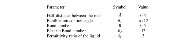
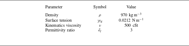
 500cSt
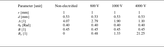

 500cSt
 600V
 1000V
 4000V
 500cSt

 500cSt
 600V

 5cSt
 3000V


 Hb
 A
 A=4
 A=6
 A=10.3

 Be=0
 A=3
 t=100
 t=0.05
 0.1
 0.2
 0.4
 0.8
 F+G
 θ1
 θ2
 α1
 α2
 θ0
 Hb

 A=4

 500cSt
 (a) t=0.0
 (b) t=2.5
 (c) t=5.0
 (d) t=20.0

 500cSt
 500cSt

 y
 500cSt
 y

 Hb
 θ0=40∘
 θ0
 θ0≲30∘


 Open access

