
1 Introduction
In the 1970s, Townsend (Reference Townsend1976) proposed a conceptual model describing the multi-scale nature of fluid motions in wall-bounded turbulence. He conjectured that the logarithmic region of wall turbulence is populated by a collection of randomly distributed momentum-carrying motions (or eddies) with their roots attached to the ‘wall’ (the near-wall region). Townsend (Reference Townsend1976) further hypothesised that the population density of the eddies decays proportionally to the distance to the wall ( $y$), and that their sizes scaled with
 $y$. The model was extended by Perry and co-authors (Perry & Chong Reference Perry and Chong1982; Perry, Henbest & Chong Reference Perry, Henbest and Chong1986; Perry & Marusic Reference Perry and Marusic1995) and has been recently reviewed by Marusic & Monty (Reference Marusic and Monty2019). A growing number of studies have supported the existence of the attached eddies in wall-bounded turbulence (e.g. Lozano-Durán, Flores & Jiménez Reference Lozano-Durán, Flores and Jiménez2012; Hwang Reference Hwang2015; Hellström, Marusic & Smits Reference Hellström, Marusic and Smits2016; Hwang & Bengana Reference Hwang and Bengana2016; Baars, Hutchins & Marusic Reference Baars, Hutchins and Marusic2017; Hwang & Sung Reference Hwang and Sung2018, Reference Hwang and Sung2019; Cheng et al. Reference Cheng, Li, Lozano-Durán and Liu2019; Yang, Willis & Hwang Reference Yang, Willis and Hwang2019; Baars & Marusic Reference Baars and Marusic2020; Hu, Yang & Zheng Reference Hu, Yang and Zheng2020) or complemented the original picture by Townsend (Davidson, Nickels & Krogstad Reference Davidson, Nickels and Krogstad2006; Mizuno & Jiménez Reference Mizuno and Jiménez2011; Dong et al. Reference Dong, Lozano-Durán, Sekimoto and Jiménez2017; Mouri Reference Mouri2017; Lozano-Durán & Bae Reference Lozano-Durán and Bae2019).
Under the attached-eddy model framework, the turbulence intensities can be predicted as
 $$\begin{eqnarray}\displaystyle & \displaystyle \langle u^{+2}\rangle =-A_{1}\ln (y/h)+B_{1}, & \displaystyle\end{eqnarray}$$
 $$\begin{eqnarray}\displaystyle & \displaystyle \langle w^{+2}\rangle =-C_{1}\ln (y/h)+D_{1}, & \displaystyle\end{eqnarray}$$
 $$\begin{eqnarray}\displaystyle & \displaystyle \langle v^{+2}\rangle =E_{1}, & \displaystyle\end{eqnarray}$$
 $u$,
 $w$ and
 $v$ are the streamwise, spanwise and wall-normal velocity fluctuations, respectively,
 $h$ is the boundary-layer thickness (or channel half-height) and
 $A_{1}$,
 $B_{1}$,
 $C_{1}$,
 $D_{1}$ and
 $E_{1}$ are constants. The superscript
 $+$ denotes normalisation in wall units. By assuming that the probability density function (p.d.f.) of
 $u$ is Gaussian, Meneveau & Marusic (Reference Meneveau and Marusic2013) extended (1.1a) to high-order moments and showed that a similar logarithmic scaling holds for the
 $2p$th moment
 $$\begin{eqnarray}\langle u^{+2p}\rangle ^{1/p}=-A_{p}\ln (y/h)+B_{p}.\end{eqnarray}$$
Yang et al. (Reference Yang, Baidya, Lv and Marusic2018) and Mehrez et al. (Reference Mehrez, Philip, Yamamoto and Tsuji2019) found that the  $2p$th moment of
 $w$ also follows the logarithmic scaling according to the attached-eddy model
 $$\begin{eqnarray}\langle w^{+2p}\rangle ^{1/p}=-C_{p}\ln (y/h)+D_{p}.\end{eqnarray}$$
The constants  $A_{p}$,
 $B_{p}$,
 $C_{p}$ and
 $D_{p}$ depend on the number
 $p$.
The logarithmic decay of the statistical moments with respect to  $y$ is considered to be one of the most compelling indicators in favour of the attached-eddy model, and its validity has been assessed in numerous studies by Hultmark et al. (Reference Hultmark, Vallikivi, Bailey and Smits2012), Marusic et al. (Reference Marusic, Monty, Hultmark and Smits2013), Meneveau & Marusic (Reference Meneveau and Marusic2013), Sillero, Jiménez & Moser (Reference Sillero, Jiménez and Moser2013), Lee & Moser (Reference Lee and Moser2015), Hu & Zheng (Reference Hu and Zheng2018) and Yamamoto & Tsuji (Reference Yamamoto and Tsuji2018), among others. Hultmark et al. (Reference Hultmark, Vallikivi, Bailey and Smits2012) tested the scaling in (1.1a) by measuring turbulent pipe flows at
 $Re_{\unicode[STIX]{x1D70F}}\geqslant 20\,000$. Yamamoto & Tsuji (Reference Yamamoto and Tsuji2018) reported the logarithmic variations of the streamwise velocity fluctuations in the direct numerical simulation (DNS) of turbulent channel flows up to
 $Re_{\unicode[STIX]{x1D70F}}=8000$. Meneveau & Marusic (Reference Meneveau and Marusic2013) found that high-order moments obey (1.2), from
 $2p=4$ to
 $2p=10$, in turbulent boundary layers at
 $Re_{\unicode[STIX]{x1D70F}}>7300$. However, the logarithmic decay of
 $\langle u^{+2p}\rangle ^{1/p}$ has been only observed at high Reynolds numbers,
 $Re_{\unicode[STIX]{x1D70F}}\sim O(10^{4})$, and it is practically non-existent otherwise. For
 $w$, the scaling in (1.1b) has been observed at a much lower Reynolds number compared to that of
 $u$ (Jiménez & Hoyas Reference Jiménez and Hoyas2008; Sillero et al. Reference Sillero, Jiménez and Moser2013; Lee & Moser Reference Lee and Moser2015). Very recently, Mehrez et al. (Reference Mehrez, Philip, Yamamoto and Tsuji2019) reported that the logarithmic scaling in (1.3) holds in turbulent channel flows from
 $Re_{\unicode[STIX]{x1D70F}}=1000$ to
 $Re_{\unicode[STIX]{x1D70F}}=4000$.
In the present work, we aim to answer the question: can Townsend’s wall-attached eddies be identified in low-Reynolds-number wall turbulence? If yes, this would imply that the characteristics of the wall-attached eddies could be evaluated at a lower computational and experimental cost than the numerical set-ups and experiments discussed above. Many techniques for identifying attached eddies lie on the separation of the multi-scale energetic motions in the flow. Among them, cutoff spectral filters (Mathis et al. Reference Mathis, Marusic, Chernyshenko and Hutchins2013; Chung et al. Reference Chung, Marusic, Monty, Vallikivi and Smits2015; Hwang & Sung Reference Hwang and Sung2017) and adaptive mode decomposition (AMD) (Agostini & Leschziner Reference Agostini and Leschziner2014, Reference Agostini and Leschziner2019; Wang, Pan & Wang Reference Wang, Pan and Wang2018, Reference Wang, Pan and Wang2019; Cheng et al. Reference Cheng, Li, Lozano-Durán and Liu2019) emerge as attractive candidates to extract multi-scale attached eddies. However, cutoff spectral filters suffer from artificial selection of thresholds (Wang et al. Reference Wang, Pan and Wang2018), and AMD is incapable of capturing smooth scale variations in the logarithmic region (Cheng et al. Reference Cheng, Li, Lozano-Durán and Liu2019; Agostini & Leschziner Reference Agostini and Leschziner2019).
Alternatively, the identification of flow structures based on the three-dimensional clustering of a region where a quantity of interest is intense has proven effective in elucidating eddies at multiple scales (Del Álamo et al. Reference Del Álamo, Jiménez, Zandonade and Moser2006; Lozano-Durán et al. Reference Lozano-Durán, Flores and Jiménez2012). The method has been successfully employed to investigate multi-scale vortex packets (Del Álamo et al. Reference Del Álamo, Jiménez, Zandonade and Moser2006) and the structures responsible for intense momentum transfer in turbulent channel flows (Lozano-Durán et al. Reference Lozano-Durán, Flores and Jiménez2012; Lozano-Durán & Jiménez Reference Lozano-Durán and Jiménez2014). Recently, Hwang & Sung (Reference Hwang and Sung2018) adopted the same methodology to analyse the wall-attached structures of intense velocity fluctuations in a turbulent boundary layer at  $Re_{\unicode[STIX]{x1D70F}}=980$. They examined the second-order moments carried by the structures, and concluded that the identified structures underpin Townsend’s attached eddies. In their further work (Hwang & Sung Reference Hwang and Sung2019), they reported that high-speed
 $u$-structures identified in turbulent pipe flows at
 $Re_{\unicode[STIX]{x1D70F}}=930$ and 3008 obey the logarithmic scaling with respect to
 $y$, but the same behaviour is not observed for the low-speed streaks. The asymmetry was ascribed to the differences of the local Reynolds number in the logarithmic layer.
To date, the studies on wall-attached eddies have mostly focused on turbulent flows at moderate and high Reynolds numbers, i.e.  $Re_{\unicode[STIX]{x1D70F}}\gtrsim 1000$ (Del Álamo et al. Reference Del Álamo, Jiménez, Zandonade and Moser2006; Lozano-Durán et al. Reference Lozano-Durán, Flores and Jiménez2012; Lozano-Durán & Jiménez Reference Lozano-Durán and Jiménez2014; Hwang Reference Hwang2015; Lozano-Durán & Borrell Reference Lozano-Durán and Borrell2016; Baars et al. Reference Baars, Hutchins and Marusic2017; Hwang & Sung Reference Hwang and Sung2018, Reference Hwang and Sung2019; Deshpande, Monty & Marusic Reference Deshpande, Monty and Marusic2019; Hu et al. Reference Hu, Yang and Zheng2020). In the present work, we intend to uncover the signature of Townsend’s wall-attached eddies in low-Reynolds-number wall turbulence and examine their scale-based properties in detail. We will pay special attention to the asymmetries between high- and low-speed wall-attached structures, as an increasing body of studies has reported that this asymmetric behaviour is an inherent characteristic of the velocity fluctuations. For example, Agostini & Leschziner (Reference Agostini and Leschziner2016a,Reference Agostini and Leschzinerb, Reference Agostini and Leschziner2019) stated that the modulation of the near-wall streamwise velocity fluctuations by outer large-scale motions is exceedingly asymmetric. The amplification caused by positive outer large-scale motions is much stronger than the attenuation from negative ones. Therefore, the sign of the structures is an indispensable factor for the identification and investigation of the flow structure. Additionally, the assessment of logarithmic scaling laws for the high-order moments carried by the wall-attached structures can provide further physical support in favour of the attached-eddy model, which is another topic of interest in the present study.
This paper is organised as follows. In § 2, we introduce the DNS database and structure identification method adopted in the present study. We then show the geometrical characteristics and high-order moments of the identified structures in § 3. In this section we also provide an interpretation of the asymmetric behaviour between high- and low-speed wall-attached  $u$-structures. Concluding remarks are summarised in § 4.
2 DNS database and structure identification method
The DNS database used in the present study has been extensively validated by Jiménez and co-workers (Del Álamo et al. Reference Del Álamo, Jiménez, Zandonade and Moser2004; Hoyas & Jiménez Reference Hoyas and Jiménez2006; Lozano-Durán et al. Reference Lozano-Durán, Flores and Jiménez2012; Lozano-Durán & Jiménez Reference Lozano-Durán and Jiménez2014). Four cases at  $Re_{\unicode[STIX]{x1D70F}}=186$, 358, 547 and 934 are chosen, and named Re180, Re350, Re550 and Re950, respectively. Details of the parameter settings are listed in table 1. Hereafter,
 $x$,
 $y$ and
 $z$ stand for the streamwise, wall-normal and spanwise directions, respectively.
Parameter settings in the DNSs. Here,  $L_{x}$,
 $L_{y}$ and
 $L_{z}$ are the sizes of the computational domains in the streamwise, wall-normal and spanwise direction, respectively.
 $\unicode[STIX]{x0394}x^{+}$ and
 $\unicode[STIX]{x0394}z^{+}$ denote the streamwise and spanwise grid resolutions in inner units, respectively.
 $\unicode[STIX]{x0394}y_{min}^{+}$ and
 $\unicode[STIX]{x0394}y_{max}^{+}$ are the finest and coarsest resolutions in the wall-normal direction, respectively.
 $N_{F}$ is the number of flow fields adopted to accumulate statistics.

We adopt a clustering methodology (Moisy & Jiménez Reference Moisy and Jiménez2004; Del Álamo et al. Reference Del Álamo, Jiménez, Zandonade and Moser2006; Lozano-Durán et al. Reference Lozano-Durán, Flores and Jiménez2012; Lozano-Durán & Jiménez Reference Lozano-Durán and Jiménez2014; Dong et al. Reference Dong, Lozano-Durán, Sekimoto and Jiménez2017; Osawa & Jiménez Reference Osawa and Jiménez2018; Hwang & Sung Reference Hwang and Sung2018, Reference Hwang and Sung2019; Yoon et al. Reference Yoon, Hwang, Yang and Sung2020) to identify three-dimensional structures of intense velocity fluctuations ( $u$ and
 $w$) populating the channel. The structures are defined as spatially connected regions satisfying
 $$\begin{eqnarray}\unicode[STIX]{x1D719}(x,y,z)>\unicode[STIX]{x1D6FC}\unicode[STIX]{x1D719}_{rms}(y),\end{eqnarray}$$
and
 $$\begin{eqnarray}\unicode[STIX]{x1D719}(x,y,z)<-\unicode[STIX]{x1D6FC}\unicode[STIX]{x1D719}_{rms}(y),\end{eqnarray}$$
which are termed positive (high-speed) and negative (low-speed) structures, respectively, where  $\unicode[STIX]{x1D719}$ represents either streamwise or spanwise velocity fluctuations (
 $u$ or
 $w$),
 $\unicode[STIX]{x1D719}_{rms}$ denotes the root-mean-square of
 $\unicode[STIX]{x1D719}$ and
 $\unicode[STIX]{x1D6FC}$ is a positive threshold value. The value of
 $\unicode[STIX]{x1D6FC}$ is set equal to 1.5 based on the percolation theory (Moisy & Jiménez Reference Moisy and Jiménez2004; Lozano-Durán et al. Reference Lozano-Durán, Flores and Jiménez2012; Hwang & Sung Reference Hwang and Sung2018). We have tested that the results in the present study are qualitatively similar for
 $\unicode[STIX]{x1D6FC}$ in the range of
 $1.3\leqslant \unicode[STIX]{x1D6FC}\leqslant 1.7$ (see appendix A).
Geometrically, the structures identified by (2.1) and (2.2) are characterised by  $l_{x}^{+}$,
 $l_{y}^{+}$,
 $l_{z}^{+}$ and
 $y_{min}^{+}$, where
 $l_{x}^{+}$,
 $l_{y}^{+}$ and
 $l_{z}^{+}$ denote the length, height and width, respectively, of the bounding boxes of each structure when aligned with the mean-flow direction, and
 $y_{min}^{+}$ is the minimum distance of the structure to the wall. Under the condition
 $y_{min}^{+}<1$, the structures are classified into two families: wall-attached structures if
 $y_{min}^{+}<1$, and detached structures otherwise. Accordingly, the structures are labelled as positive wall attached (
 $PA$), positive wall detached (
 $PD$), negative wall attached (
 $NA$) and negative wall detached (
 $ND$). We further used the subscripts
 $u$ and
 $w$ to distinguish the structures identified by using different velocity fluctuations.
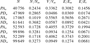
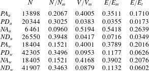
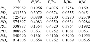
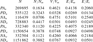
Tables 2–5 summarise the number ( $N$), number fraction (
 $N/N_{m}$), volume fraction (
 $V/V_{m}$) and energy fractions (
 $E/E_{m}$,
 $E/E_{t}$) of
 $u$- and
 $w$-structures for all cases, where
 $V=\sum (l_{x}l_{y}l_{z})$,
 $E=\sum \frac{1}{2}\unicode[STIX]{x1D719}^{2}$ and the sum is applied to different families (
 $PA$,
 $PD$,
 $NA$ or
 $ND$). The total quantities computed over all identified structures and over the whole channel are denoted by the subscripts
 $m$ and
 $t$, respectively. The results from tables 2–5 show that the number of attached structures is smaller than the detached ones, but their volume and energy are notably larger. The energy of attached structures (
 $PA$ and
 $NA$) accounts for nearly 40 % of
 $E_{t}$, whereas the energy of detached structures (
 $PD$ and
 $ND$) accounts only for 1 %–5 %. The difference suggests that wall-attached structures are representative of the energy-containing motions in turbulent flows. Consequently, in the following sections, we focus on
 $PA$ and
 $NA$ and their relationship with the predictions of the attached-eddy model.
The number ( $N$), number fraction (
 $N/N_{m}$), volume fraction (
 $V/V_{m}$) and energy fractions (
 $E/E_{m}$,
 $E/E_{t}$) of the identified
 $u$- and
 $w$-structures in Re180.

The number ( $N$), number fraction (
 $N/N_{m}$), volume fraction (
 $V/V_{m}$) and energy fractions (
 $E/E_{m}$,
 $E/E_{t}$) of the identified
 $u$- and
 $w$-structures in Re350.

The number ( $N$), number fraction (
 $N/N_{m}$), volume fraction (
 $V/V_{m}$) and energy fractions (
 $E/E_{m}$,
 $E/E_{t}$) of the identified
 $u$- and
 $w$-structures in Re550.

The number ( $N$), number fraction (
 $N/N_{m}$), volume fraction (
 $V/V_{m}$) and energy fractions (
 $E/E_{m}$,
 $E/E_{t}$) of the identified
 $u$- and
 $w$-structures in Re950.

3 Results and discussion
The statistical properties of the wall-attached  $u$- and
 $w$-structures are analysed separately in §§ 3.1 and 3.2 by using Re550. The other three cases (Re180, Re350 and Re950) are included in § 3.3 to access the Reynolds-number effects on the statistical properties of the structures. Bearing in mind the three key features of Townsend’s attached eddies: (i) their sizes are proportional to
 $y$, (ii) their population density is inversely proportional to
 $y$ and (iii) the statistical moments of the inactive parts (
 $u$ and
 $w$) follow logarithmic wall-normal scalings, we examine the properties of the structures from each of these perspectives.
3.1 The wall-attached  $u$-structures

3.1.1 Length-scale self-similarity
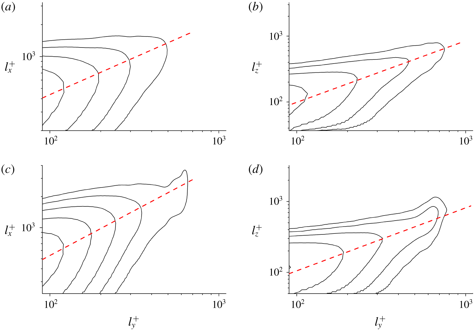
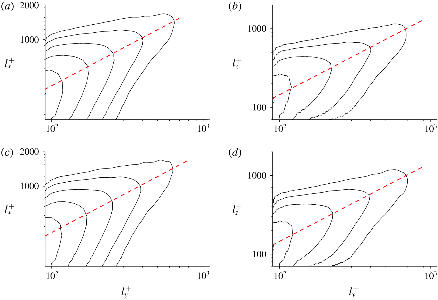
The geometrical properties of the wall-attached  $u$-structures (
 $PA_{u}$ and
 $NA_{u}$) in Re550 are examined by the joint p.d.f.s of
 $l_{x}^{+}$,
 $l_{z}^{+}$ with respect to
 $l_{y}^{+}$, as shown in figure 1. Hereafter, we mainly focus on the large-scale structures, i.e. those with
 $l_{y}^{+}>100$, whose wall-normal centres are approximately located at
 $y^{+}>50$. It can be seen that
 $l_{x}^{+}$ and
 $l_{z}^{+}$ increase with
 $l_{y}^{+}$ according to well-defined scaling laws. Nonlinear relationships are observed between
 $l_{x}^{+}$ and
 $l_{y}^{+}$, that is
 $l_{x}^{+}\propto (l_{y}^{+})^{0.70}$ for
 $PA_{u}$ and
 $l_{x}^{+}\propto (l_{y}^{+})^{0.88}$ for
 $NA_{u}$, and a linear relationship is well exhibited between
 $l_{z}^{+}$ and
 $l_{y}^{+}$. These sizes are approximately consistent with the observations in a turbulent boundary layer (Hwang & Sung Reference Hwang and Sung2018), suggesting that the geometrical self-similarity of spanwise length scales is also present in the wall turbulence even at much lower Reynolds numbers.
(a,b) Joint p.d.f.s of the length ( $l_{x}^{+}$) and width (
 $l_{z}^{+}$) of
 $PA_{u}$ in Re550 with respect to their height (
 $l_{y}^{+}$). The red dashed lines in (a,b) denote
 $l_{x}^{+}=17.41(l_{y}^{+})^{0.70}$ and
 $l_{z}^{+}=l_{y}^{+}$, respectively. (c,d) Joint p.d.f.s of the length (
 $l_{x}^{+}$) and width (
 $l_{z}^{+}$) of
 $NA_{u}$ in Re550 with respect to their height (
 $l_{y}^{+}$). The red dashed lines in (c,d) denote
 $l_{x}^{+}=9.88(l_{y}^{+})^{0.88}$ and
 $l_{z}^{+}=l_{y}^{+}$, respectively. All of these p.d.f.s are logarithmically distributed.

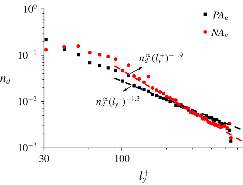
We next analyse the wall-normal decay of the population density of structures. Following Lozano-Durán et al. (Reference Lozano-Durán, Flores and Jiménez2012), we define the population density as  $n_{d}(l_{y}^{+})=N_{i}(l_{y}^{+})/(2N_{F}A)$, where
 $N_{i}(l_{y}^{+})$ is the number of structures with a given
 $l_{y}^{+}$,
 $N_{F}$ is number of the flow fields and
 $A$ represents the area of the wall
 $L_{x}\times L_{z}$. Figure 2 displays
 $n_{d}$ as a function of
 $l_{y}^{+}$. The density of structures decays as
 $n_{d}\propto (l_{y}^{+})^{-1.9}$ for
 $NA_{u}$, while for
 $PA_{u}$ the density is well approximated by
 $n_{d}\propto (l_{y}^{+})^{-1.3}$. Since the expected theoretical estimation of
 $n_{d}$ obeys
 $n_{d}\propto (l_{y}^{+})^{-1}$ (Perry & Chong Reference Perry and Chong1982; Perry et al. Reference Perry, Henbest and Chong1986), the population density of
 $PA_{u}$ follows more closely the prediction of the attached-eddy theory than that of
 $NA_{u}$.
The population density ( $n_{d}$) of
 $PA_{u}$ and
 $NA_{u}$ as a function of
 $l_{y}^{+}$ in Re550. The red and black dashed lines represent
 $n_{d}\propto (l_{y}^{+})^{-1.9}$ and
 $n_{d}\propto (l_{y}^{+})^{-1.3}$, respectively.

3.1.2 Logarithmic wall-normal scaling of the statistical moments
To evaluate the scaling of the statistical moments and further examine the differences between  $PA_{u}$ and
 $NA_{u}$, we define the conditional statistical moment of
 $u$ as
 $$\begin{eqnarray}\langle u_{a}^{2p+}\rangle ^{1/p}(y,l_{y}^{+})=\left\{\frac{1}{N_{u}(y,l_{y}^{+})}\mathop{\sum }_{i=1}^{N_{u}(y,l_{y}^{+})}\left[\frac{u_{i}(x,y,z)|_{l_{y}^{+}}}{u_{\unicode[STIX]{x1D70F}}}\right]^{2p}\right\}^{1/p},\end{eqnarray}$$
where  $N_{u}(y,l_{y}^{+})$ denotes the number of grid points belonging to a structure with
 $l_{y}^{+}$ at a given
 $y$, and
 $u_{i}(x,y,z)|_{l_{y}^{+}}$ denotes the streamwise velocity fluctuation of the
 $i$th grid point of the structure. In this manner,
 $\langle u_{a}^{2p+}\rangle ^{1/p}$ represents the
 $2p$th root of the streamwise velocity moment carried by the structures with a given scale
 $l_{y}^{+}$.
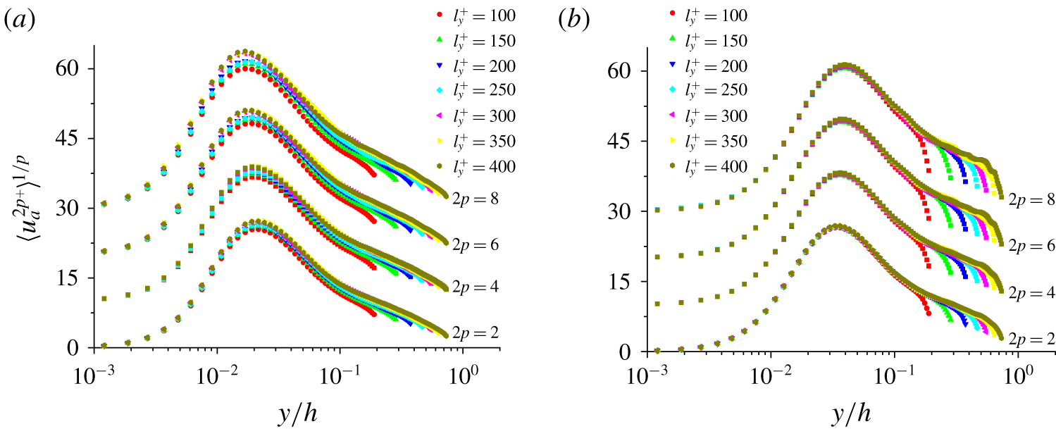
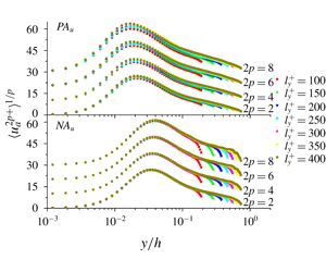
Figure 3 shows the profiles of  $\langle u_{a}^{2p+}\rangle ^{1/p}$, from
 $2p=2$ to
 $2p=8$, carried by structures with several selected
 $l_{y}^{+}$ in Re550. The figure reveals that, for increasing
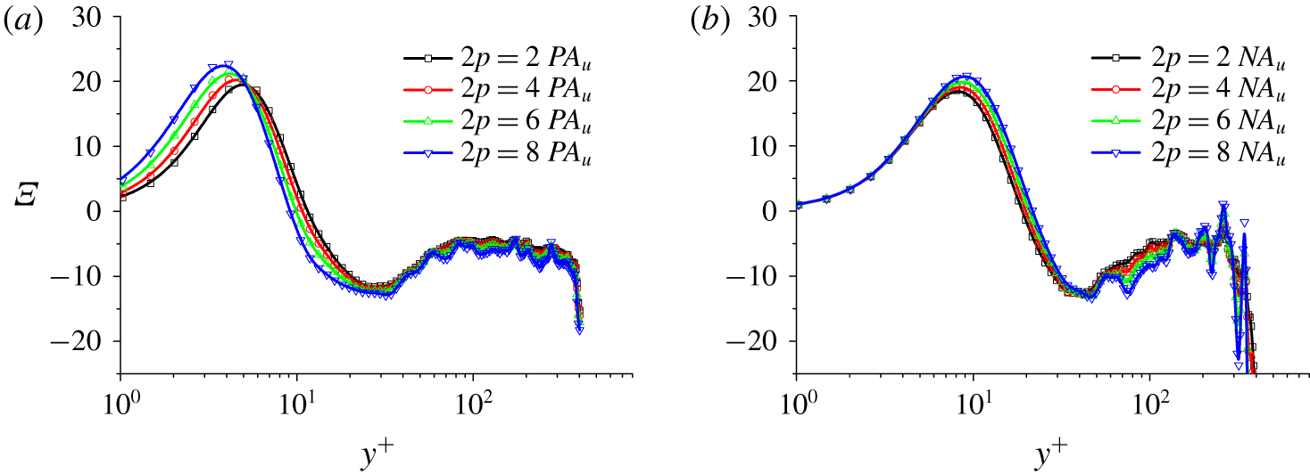
 $l_{y}^{+}$, the profiles tend to decay logarithmically. To quantify the logarithmic decay in a systematic manner, we define the indicator function
 $\unicode[STIX]{x1D6EF}=y(\unicode[STIX]{x2202}\langle u_{a}^{2p+}\rangle ^{1/p}/\unicode[STIX]{x2202}y)$. Figure 4 shows the value of
 $\unicode[STIX]{x1D6EF}$ as a function of
 $y^{+}$, for the structures with
 $l_{y}^{+}=400$. Comparatively well-defined plateaus are observed for
 $PA_{u}$ regardless of the value of
 $p$. On the contrary,
 $\unicode[STIX]{x1D6EF}$ does not approach a constant value for
 $NA_{u}$. This phenomenon, together with the observations in § 3.1.1, suggests that
 $PA_{u}$ are more inclined to behave akin to ideal wall-attached eddies.
Wall-normal variations of the  $2p$th root of moments of the streamwise velocity fluctuations carried by
 $PA_{u}$ (a) and
 $NA_{u}$ (b) with several selected wall-normal heights in Re550. The profiles of the 4th, 6th and 8th roots of the moments are shifted upward by
 $\unicode[STIX]{x1D6E5}\langle u_{a}^{4+}\rangle ^{1/2}=10$,
 $\unicode[STIX]{x1D6E5}\langle u_{a}^{6+}\rangle ^{1/3}=20$ and
 $\unicode[STIX]{x1D6E5}\langle u_{a}^{8+}\rangle ^{1/4}=30$, respectively.

Wall-normal variations of the corresponding indicator functions of the statistical moments from  $2p=2$ to
 $2p=8$ for
 $PA_{u}$ (a) and
 $NA_{u}$ (b) with
 $l_{y}^{+}=400$ in Re550.

3.1.3 Inner peaks of the statistical moments of the streamwise velocity fluctuation
Another consequence of the attached-eddy model is the increase of the inner peaks of the second-order moment of  $u$ as
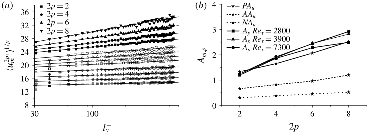
 $\ln (Re_{\unicode[STIX]{x1D70F}})$, which has been validated in previous numerical and experimental studies (Marusic & Kunkel Reference Marusic and Kunkel2003; Hoyas & Jiménez Reference Hoyas and Jiménez2006; Lee & Moser Reference Lee and Moser2015; Marusic, Baars & Hutchins Reference Marusic, Baars and Hutchins2017). By assuming that the inner peaks are the sole outcome of the wall-attached eddies residing in the logarithmic region, Meneveau & Marusic (Reference Meneveau and Marusic2013) derived a generalised formula for the inner peaks of the statistical moments of
 $u$,
 $$\begin{eqnarray}\langle u_{m}^{2p+}\rangle ^{1/p}\sim A_{p}\ln Re_{\unicode[STIX]{x1D70F}},\end{eqnarray}$$
where the coefficients  $A_{p}$ are identical to those in (1.2), and represent the growth rates of the inner peaks.
Considering that  $l_{y}^{+}$ can be interpreted as local
 $Re_{\unicode[STIX]{x1D70F}}$, by using the case of Re550, we further show in figure 5(a) the variations of
 $\langle u_{m}^{2p+}\rangle ^{1/p}$ as a function of
 $l_{y}^{+}$. For comparison, the wall-attached
 $u$-structures satisfying both (2.1) and (2.2), are also included and named
 $AA_{u}$, where
 $AA_{u}=PA_{u}+NA_{u}$. The inner peaks increase logarithmically with
 $l_{y}^{+}$ both for the high- and low-speed wall-attached
 $u$-structures, although the associated growth rates are different. In figure 5(b), the growth rates are compared with the high-Reynolds-number experimental results by Meneveau & Marusic (Reference Meneveau and Marusic2013). The growth rates of
 $PA_{u}$ are approximately in agreement with the experimental data, while the growth rates of
 $AA_{u}$ are approximately half of those of
 $PA_{u}$ due to the relatively smaller values of
 $NA_{u}$.
(a) Variations of inner peaks ( $\langle u_{m}^{2p+}\rangle ^{1/p}$) as a function of
 $l_{y}^{+}$ in Re550. The solid symbols denote
 $PA_{u}$, hollow symbols denote
 $AA_{u}$ and hollow symbols with ‘
 $+$’ denote
 $NA_{u}$. The symbols of
 $AA_{u}$ and
 $NA_{u}$ are shifted downward by
 $\unicode[STIX]{x1D6E5}\langle u_{m}^{2p+}\rangle ^{1/p}=5$ and
 $\unicode[STIX]{x1D6E5}\langle u_{m}^{2p+}\rangle ^{1/p}=12$, respectively. The solid lines are the fitting curves. (
 $b$) Variations of the growth rates of the inner peaks (
 $A_{m,p}$) as a function of the moment order
 $2p$ in Re550, compared with the
 $A_{p}$ obtained from experiments (Meneveau & Marusic Reference Meneveau and Marusic2013).

Recalling that both in experimental measurements and simulations the growth rates of the inner peaks are found to be lower than the theoretical predictions of  $A_{p}$ in (3.2), an empirical factor
 $(1-\unicode[STIX]{x1D6FE})$ was introduced to correct
 $A_{p}$ with
 $\unicode[STIX]{x1D6FE}=0.5$ (Klewicki, Fife & Wei Reference Klewicki, Fife and Wei2009; Alfredsson, Segalini & Örlü Reference Alfredsson, Segalini and Örlü2011; Meneveau & Marusic Reference Meneveau and Marusic2013; Marusic et al. Reference Marusic, Baars and Hutchins2017). Note that, in these studies, no high- and low-speed scale separation has been conducted, similar to
 $AA_{u}$ in the present study. The results from figure 5 suggest that, although the features of the inner peaks of
 $AA_{u}$ are consistent with the experimental results for the empirical correction on
 $A_{p}$, the positive structures are again more in line with the theoretical predictions of the attached-eddy model.
3.1.4 An interpretation of the asymmetric behaviour between $PA_{u}$ and $NA_{u}$


The comparison of  $PA_{u}$ and
 $NA_{u}$ has shown that the former follow more closely the theoretical predictions of the attached-eddy model framework. Hwang & Sung (Reference Hwang and Sung2019) observed a similar behaviour for the scale-based streamwise velocities in turbulent pipe flows up to
 $Re_{\unicode[STIX]{x1D70F}}=3008$. In their work, they attributed this phenomenon to the differences in the local
 $Re_{\unicode[STIX]{x1D70F}}$ conditioned to the presence of high- and low-speed streaks. In that respect, high-speed streaks are locally associated with higher Reynolds numbers, which was used to justify the emergence of logarithmic trends in quantities conditioned to the aforementioned structures. However, a similar analysis using our data (Re550) indicates that the friction Reynolds number conditioned to the presence of high-speed streaks is at most
 $Re_{\unicode[STIX]{x1D70F}}\approx 1000$, which is still too low to explain the appearance of the logarithmic trends in
 $PA_{u}$ discussed in previous subsections. Therefore, our results suggest that the differences in the local Reynolds number are probably not essential to understand the asymmetries between
 $NA_{u}$ and
 $PA_{u}$ reported above.
We provide an alternative interpretation of the differences between  $PA_{u}$ and
 $NA_{u}$ based on the asymmetries of the fluid advected by sweeps and ejections. We measure
 $u$ and
 $v$ within the interior region of an identified structure to examine the averaged advection of the structure from the perspective of the quadrant decomposition (Wallace Reference Wallace2016). For the wall-attached
 $u$-structures (
 $PA_{u}$ and
 $NA_{u}$) with
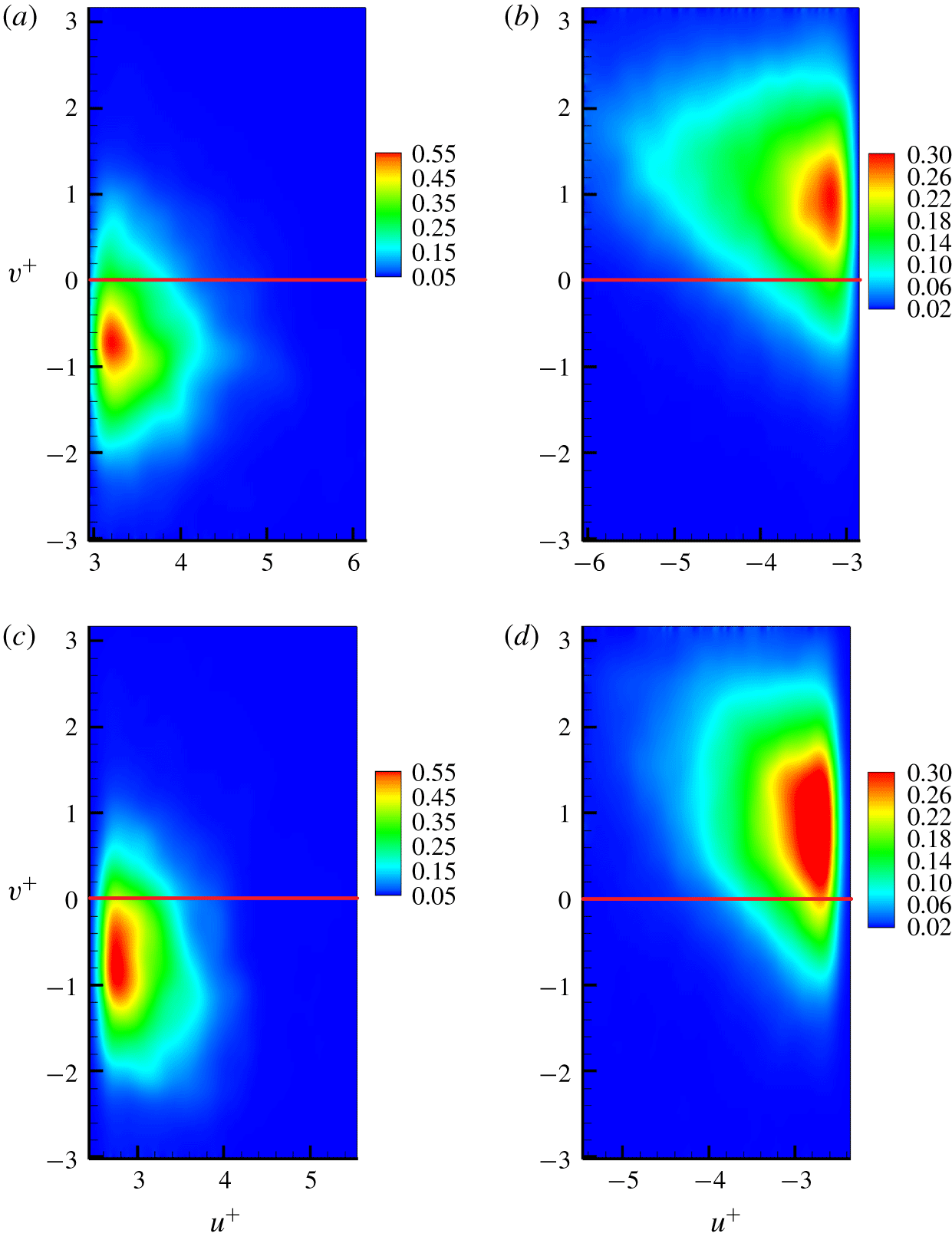
 $l_{y}^{+}=400$, the joint p.d.f.s of
 $u^{+}$ and
 $v^{+}$ at
 $y/h=0.1$ and
 $y/h=0.2$ are displayed in figure 6. The results reveal that
 $PA_{u}$ with
 $l_{y}^{+}=400$ are associated with sweep events (
 $u^{+}>0$,
 $v^{+}<0$), while
 $NA_{u}$ with
 $l_{y}^{+}=400$ are strongly correlated with the ejection events (
 $u^{+}<0$,
 $v^{+}>0$). This observation holds for varying
 $l_{y}^{+}$.
(a,b) The joint p.d.f.s of  $u^{+}$ and
 $v^{+}$ at
 $y/h=0.1$ for
 $PA_{u}$ (a) and
 $NA_{u}$ (b) with
 $l_{y}^{+}=400$ in Re550. (c,d) The joint p.d.f.s of
 $u^{+}$ and
 $v^{+}$ at
 $y/h=0.2$ for
 $PA_{u}$ (c) and
 $NA_{u}$ (d) with
 $l_{y}^{+}=400$ in Re550. The red lines denote
 $v^{+}=0$.

Consequently,  $PA_{u}$ are predominantly dominated by low shear flow from the upper region of the boundary layer, while
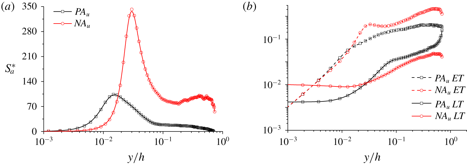
 $NA_{u}$ are strongly influenced by the higher shear and turbulence intensities of the near-wall region. The difference can be quantified more precisely using the Corrsin shear parameter (Corrsin Reference Corrsin1958)
 $S^{\ast }=SL_{\unicode[STIX]{x1D700}}/q$, which not only characterises the strength of the mean shear
 $S$, controlling the dynamics of eddies with integral length scale
 $L_{\unicode[STIX]{x1D700}}$ and turbulent kinetic energy
 $q^{2}$, but also stands for the ratio of the equilibration time
 $L_{\unicode[STIX]{x1D700}}/q$ (denoted as ET hereafter) and the life time
 $1/S$ (denoted as LT hereafter) of the eddies (Jiménez Reference Jiménez2018).
To shed light on the difference in the mean shear between  $PA_{u}$ and
 $NA_{u}$, we define the conditional (scale-based) mean streamwise velocity, turbulent kinetic energy and dissipation as
 $$\begin{eqnarray}\displaystyle & \displaystyle \langle U_{a}\rangle (y,l_{y}^{+})=\left\{\frac{1}{N_{u}(y,l_{y}^{+})}\mathop{\sum }_{i=1}^{N_{u}(y,l_{y}^{+})}U_{i}(x,y,z)|_{l_{y}^{+}}\right\}, & \displaystyle\end{eqnarray}$$
 $$\begin{eqnarray}\displaystyle & \displaystyle \langle q_{a}^{2}\rangle (y,l_{y}^{+})=\left\{\frac{1}{N_{u}(y,l_{y}^{+})}\mathop{\sum }_{i=1}^{N_{u}(y,l_{y}^{+})}q_{i}^{2}(x,y,z)|_{l_{y}^{+}}\right\}, & \displaystyle\end{eqnarray}$$
 $$\begin{eqnarray}\displaystyle & \displaystyle \langle \unicode[STIX]{x1D716}_{a}\rangle (y,l_{y}^{+})=\left\{\frac{1}{N_{u}(y,l_{y}^{+})}\mathop{\sum }_{i=1}^{N_{u}(y,l_{y}^{+})}\unicode[STIX]{x1D716}_{i}(x,y,z)|_{l_{y}^{+}}\right\}, & \displaystyle\end{eqnarray}$$
respectively, where  $U_{i}(x,y,z)|_{l_{y}^{+}}$,
 $q_{i}^{2}(x,y,z)|_{l_{y}^{+}}$ and
 $\unicode[STIX]{x1D716}_{i}(x,y,z)|_{l_{y}^{+}}$ denote instantaneous streamwise velocity, turbulent kinetic energy and dissipation of the
 $i$th grid point of the structure with size
 $l_{y}^{+}$, respectively. The mean shear is calculated by
 $S_{a}(y)|_{l_{y}^{+}}=\unicode[STIX]{x2202}\langle U_{a}\rangle /\unicode[STIX]{x2202}y|_{l_{y}^{+}}$, and the conditional shear parameter is expressed as
 $$\begin{eqnarray}S_{a}^{\ast }(y)=\frac{S_{a}\langle q_{a}^{2}\rangle }{\langle \unicode[STIX]{x1D716}_{a}\rangle }.\end{eqnarray}$$
Figure 7(a) shows the variations of  $S_{a}^{\ast }$ as a function of
 $y/h$ for
 $PA_{u}$ and
 $NA_{u}$ with
 $l_{y}^{+}=400$ in Re550. The shear parameter conditioned to
 $NA_{u}$ is visibly larger than that of
 $PA_{u}$ for
 $y/h>0.02$. This suggests that
 $NA_{u}$ originate under the strong shear conditions of the near-wall region, while
 $PA_{u}$ are controlled by the low shear flow in the upper domain of the boundary layer. Moreover, the wall-normal variations of ET and LT of
 $PA_{u}$ and
 $NA_{u}$ with
 $l_{y}^{+}=400$ are displayed in figure 7(b). For
 $PA_{u}$, the values of ET and LT are closer to each other than those of
 $NA_{u}$ when
 $y/h>0.03$. Consequently, it can be hypothesised that the flow associated with
 $NA_{u}$ is less likely to equilibrate during their life time to obey the logarithmic trends than that of
 $PA_{u}$, which is consistent with the asymmetrical features observed between
 $PA_{u}$ and
 $NA_{u}$.
(a) Wall-normal variations of the conditional shear parameter ( $S_{a}^{\ast }$) carried by
 $PA_{u}$ and
 $NA_{u}$ with
 $l_{y}^{+}=400$ in Re550. (b) Wall-normal variations of the life time and equilibration time of
 $PA_{u}$ and
 $NA_{u}$ with
 $l_{y}^{+}=400$ in Re550.

Finally, the trends for the inner peaks shown in figure 5 can also be interpreted from the sweep/ejection viewpoint. The inner peaks of  $PA_{u}$ arise from the top-to-bottom wall interactions of sweep events. In this context, it is reasonable to assume that the
 $\ln (Re_{\unicode[STIX]{x1D70F}})$ growth rate of the inner peak is mainly a consequence of the outer flow transported by
 $PA_{u}$.
3.2 The wall-attached $w$-structures

The spanwise fluctuating velocity represents another inactive component of the wall-attached eddies, which is also hypothesised to be geometrically self-similar. The length scales of wall-attached  $w$-structures (
 $PA_{w}$ and
 $NA_{w}$) are characterised by the joint p.d.f.s of
 $l_{x}^{+}$,
 $l_{z}^{+}$ with respect to
 $l_{y}^{+}$, which are shown in figure 8 using the case of Re550. Similarly to the observations for wall-attached
 $u$-structures, there is on average a nonlinear relationship between
 $l_{x}^{+}$ and
 $l_{y}^{+}$, whereas
 $l_{z}^{+}$ and
 $l_{y}^{+}$ are linearly proportional, both for
 $PA_{w}$ and
 $NA_{w}$. The results support the geometrical self-similarity of wall-attached
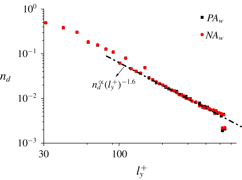
 $w$-structures. The population densities of the wall-attached
 $w$-structures is displayed in figure 9. The densities decay as
 $n_{d}\propto (l_{y}^{+})^{-1.6}$, similarly for
 $PA_{w}$ and
 $NA_{w}$, unlike the trends obtained for
 $u$-structures. The geometrical and distributional features suggest no asymmetry between
 $PA_{w}$ and
 $NA_{w}$, which is in line with expectations since the flow is statistically homogeneous in the spanwise direction. Moreover, one inevitable result of the symmetry, in stark contrast to the
 $u$-structures, is that the tendency of the
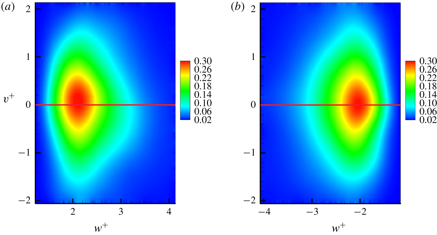
 $w$-structures associated with sweep and ejection events is absent. Figure 10 shows the joint p.d.f.s of
 $w^{+}$ and
 $v^{+}$ at
 $y/h=0.2$ conditioned to
 $PA_{w}$ and
 $NA_{w}$ with
 $l_{y}^{+}=400$ in Re550. The p.d.f.s are approximately symmetrical along
 $v^{+}=0$, which suggests that
 $PA_{w}$ and
 $NA_{w}$ connect with the sweep and ejection events in the same manner, as expected.
Given the symmetries reported between  $PA_{w}$ and
 $NA_{w}$, the statistical moments of
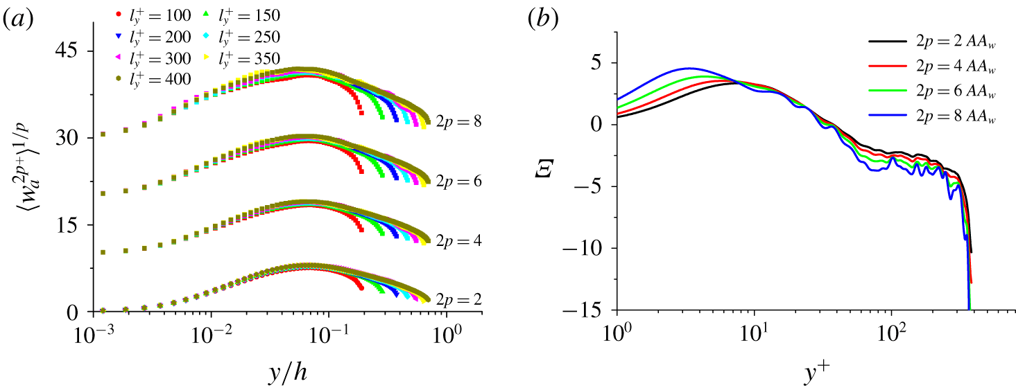
 $w$ are examined without distinguishing their signs. We define
 $AA_{w}$ as
 $AA_{w}=PA_{w}+NA_{w}$ and follow the definition of
 $\langle u_{a}^{2p+}\rangle ^{1/p}$ in (3.1). The conditional statistical moments of
 $w$,
 $\langle w_{a}^{2p+}\rangle ^{1/p}$, are shown in figure 11(a). As
 $l_{y}^{+}$ increases, the moments of
 $w$ tend to decay logarithmically. Figure 11(b) shows the corresponding indicator function
 $\unicode[STIX]{x1D6EF}$ to assess the logarithmic scaling. The values of
 $\unicode[STIX]{x1D6EF}$ are roughly constant in the range of
 $80<y^{+}<160$, which indicates that the wall-attached
 $w$-structures behave similarly to ideal attached eddies. Nevertheless, the plateaus are less defined than those observed for
 $u$-structures. This phenomenon appears to contradict the observations of Lee & Moser (Reference Lee and Moser2015), who reported that the logarithmic decay of spanwise turbulence intensity is more robust than that of streamwise turbulence intensity. This is presumably caused by the inclusion of
 $NA_{u}$ in the streamwise turbulence intensity. As an aside, the logarithmic scaling of
 $AA_{w}$ is more notable as
 $Re_{\unicode[STIX]{x1D70F}}$ increases, which will be reported in § 3.3.
(a,b) Joint p.d.f.s of the length ( $l_{x}^{+}$) and width (
 $l_{z}^{+}$) of
 $PA_{w}$ in Re550 with respect to their height (
 $l_{y}^{+}$). The red dashed lines in (a,b) denote
 $l_{x}^{+}=15.65(l_{y}^{+})^{0.70}$ and
 $l_{z}^{+}=1.45l_{y}^{+}$, respectively. (c,d) Joint p.d.f.s of the length (
 $l_{x}^{+}$) and width (
 $l_{z}^{+}$) of
 $NA_{w}$ in Re550 with respect to their height (
 $l_{y}^{+}$). The red dashed lines in (c,d) denote
 $l_{x}^{+}=15.65(l_{y}^{+})^{0.70}$ and
 $l_{z}^{+}=1.45l_{y}^{+}$, respectively. All of these p.d.f.s are logarithmically distributed.

The population density ( $n_{d}$) of
 $PA_{w}$ and
 $NA_{w}$ in Re550 as a function of
 $l_{y}^{+}$. The black dashed line represents
 $n_{d}\propto (l_{y}^{+})^{-1.6}$.

The joint p.d.f.s of  $w^{+}$ and
 $v^{+}$ at
 $y/h=0.2$ for
 $PA_{w}$ (a) and
 $NA_{w}$ (b) with
 $l_{y}^{+}=400$ in Re550. The red lines denote
 $v^{+}=0$.

(a) Wall-normal variations of the  $2p$th root of the moments of the spanwise velocity fluctuations carried by
 $AA_{w}$ with several selected wall-normal heights in Re550. The profiles of the 4th, 6th and 8th roots of moments are shifted upward by
 $\unicode[STIX]{x1D6E5}\langle w_{a}^{4+}\rangle ^{1/2}=10$,
 $\unicode[STIX]{x1D6E5}\langle w_{a}^{6+}\rangle ^{1/3}=20$ and
 $\unicode[STIX]{x1D6E5}\langle w_{a}^{8+}\rangle ^{1/4}=30$, respectively. (b) Wall-normal variations of the corresponding indicator functions of the statistical moments from
 $2p=2$ to
 $2p=8$ for
 $AA_{w}$ with
 $l_{y}^{+}=400$ in Re550.

3.3 Reynolds-number effects on the statistical properties of the structures
In this subsection, the other three cases (Re180, Re350 and Re950) are included to assess the Reynolds-number effects on the statistical properties of the wall-attached  $u$- and
 $w$-structures.
3.3.1 The wall-attached $u$-structures

We first focus on the statistical properties of the wall-attached  $u$-structures. As for the geometrical features, the relationships between
 $l_{x}^{+}$,
 $l_{z}^{+}$ and
 $l_{y}^{+}$ can be expressed as
 $l_{x}^{+}\propto (l_{y}^{+})^{\unicode[STIX]{x1D6FE}_{1}}$ and
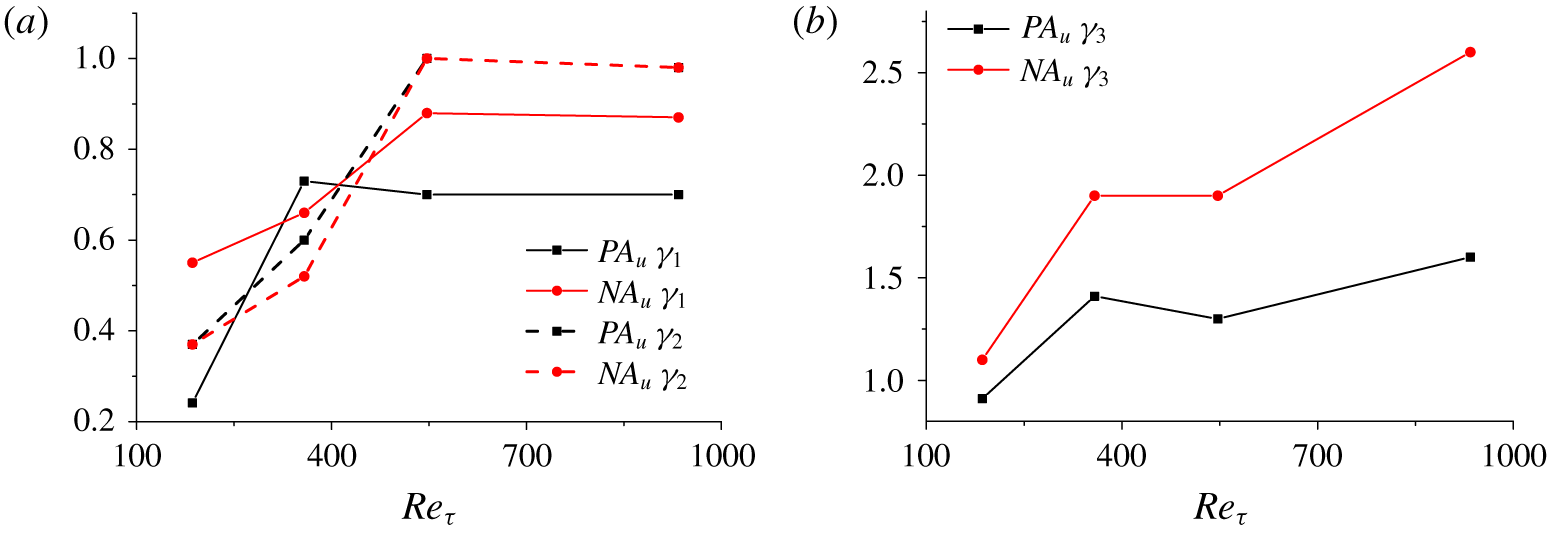
 $l_{z}^{+}\propto (l_{y}^{+})^{\unicode[STIX]{x1D6FE}_{2}}$, respectively. Figure 12(a) shows the variations of
 $\unicode[STIX]{x1D6FE}_{1}$ and
 $\unicode[STIX]{x1D6FE}_{2}$ as a function of
 $Re_{\unicode[STIX]{x1D70F}}$. Note that only the structures with
 $l_{y}^{+}>100$ are taken into account. As
 $Re_{\unicode[STIX]{x1D70F}}$ increases,
 $\unicode[STIX]{x1D6FE}_{1}$ seems to converge to a constant value; whereas remarkable asymmetries are always observed between
 $PA_{u}$ and
 $NA_{u}$, regardless of
 $Re_{\unicode[STIX]{x1D70F}}$. The value of
 $\unicode[STIX]{x1D6FE}_{2}$ is in close proximity that when
 $Re_{\unicode[STIX]{x1D70F}}\geqslant 547$, indicating the self-similarity of the
 $u$-structures. The population density of the structures is represented by
 $n_{d}\propto (l_{y}^{+})^{-\unicode[STIX]{x1D6FE}_{3}}$, and the variations of the index
 $\unicode[STIX]{x1D6FE}_{3}$ are shown in figure 12(b) as a function of
 $Re_{\unicode[STIX]{x1D70F}}$. As seen, the values of
 $\unicode[STIX]{x1D6FE}_{3}$ for
 $PA_{u}$ are invariably close to the predictions of the attached-eddy model.
(a) The variations of  $\unicode[STIX]{x1D6FE}_{1}$ and
 $\unicode[STIX]{x1D6FE}_{2}$ as a function of
 $Re_{\unicode[STIX]{x1D70F}}$ for
 $u$-structures. (b) The variations of
 $\unicode[STIX]{x1D6FE}_{3}$ as a function of
 $Re_{\unicode[STIX]{x1D70F}}$ for
 $u$-structures.

Wall-normal variations of the corresponding indicator function of the second-order moment for  $PA_{u}$ (a) and
 $NA_{u}$ (b) with selected
 $l_{y}^{+}$ for all cases.

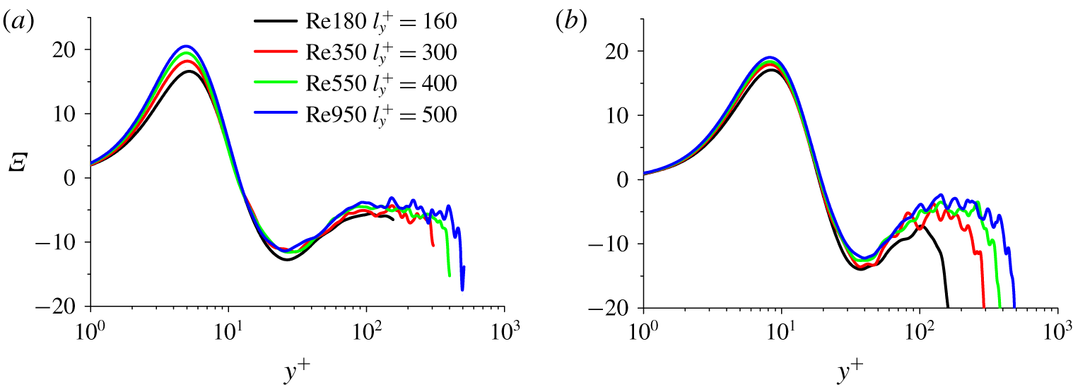
We next examine Reynolds-number effects on the statistical moments of the  $u$-structures. Figure 13 shows the corresponding indicator function
 $\unicode[STIX]{x1D6EF}$ of the second-order moment of the
 $u$-structures for all cases. It can be seen that comparatively well-defined plateaus are observed for
 $PA_{u}$. The plateaus start from
 $y^{+}\approx 80$, which corresponds to the lower limit of the logarithmic region (Jiménez Reference Jiménez2018; Baars & Marusic Reference Baars and Marusic2020). For
 $NA_{u}$, however,
 $\unicode[STIX]{x1D6EF}$ does not approach a constant value. Note that the wrinkles in figure 13 may be caused by a lack of DNS samples. To the authors knowledge, this is the first time the logarithmic decay of the streamwise turbulence intensity at such low Reynolds numbers (
 $Re_{\unicode[STIX]{x1D70F}}\approx 180{-}550$) has been shown.
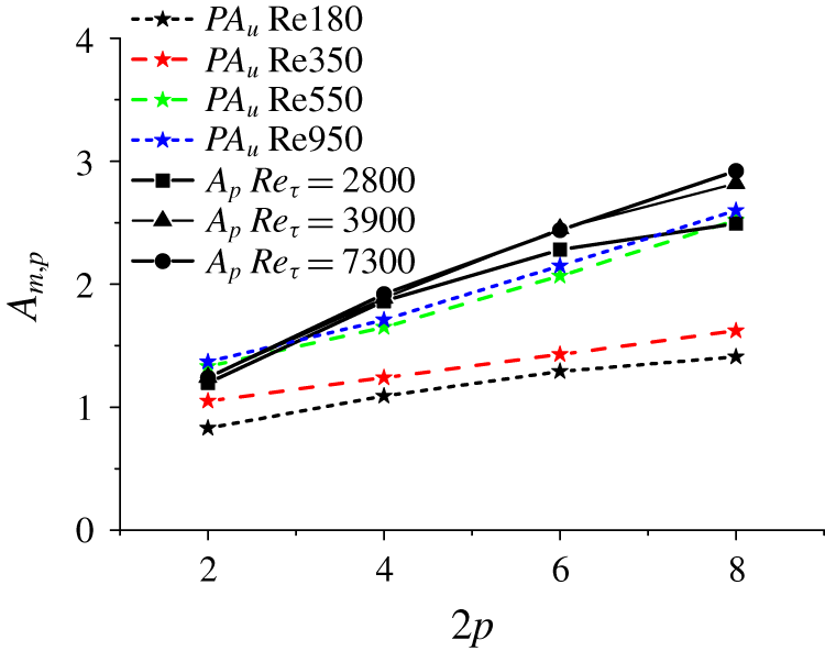
Variations of the growth rates of the inner peaks ( $A_{m,p}$) associated with
 $PA_{u}$ at different Reynolds numbers as a function of the moment order
 $2p$, compared with the
 $A_{p}$ obtained from experiments (Meneveau & Marusic Reference Meneveau and Marusic2013).

Finally, the growth rates of the inner peaks associated with  $PA_{u}$ at different Reynolds number are examined and displayed in figure 14. The growth rates of the inner peaks are increased with the Reynolds number and tend to be consistent with the experimental results when
 $Re_{\unicode[STIX]{x1D70F}}\geqslant 547$. The mismatches in Re180 and Re350 are probably related to the viscous effect, which plays a non-negligible role in outer flow transport.
3.3.2 The wall-attached $w$-structures

We examine the Reynolds-number effects on statistical properties of the wall-attached  $w$-structures. Due to the lack of asymmetry between
 $PA_{w}$ and
 $NA_{w}$, we only take
 $AA_{w}$ (
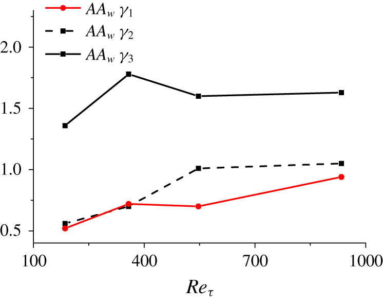
 $AA_{w}=PA_{w}+NA_{w}$) into account. Figure 15 shows the variations of
 $\unicode[STIX]{x1D6FE}_{1}$,
 $\unicode[STIX]{x1D6FE}_{2}$ and
 $\unicode[STIX]{x1D6FE}_{3}$ as functions of
 $Re_{\unicode[STIX]{x1D70F}}$ for
 $AA_{w}$. As
 $Re_{\unicode[STIX]{x1D70F}}$ increases, the values of
 $\unicode[STIX]{x1D6FE}_{1}$ and
 $\unicode[STIX]{x1D6FE}_{2}$ tend to be one, indicating the formation of the self-similarity. For
 $\unicode[STIX]{x1D6FE}_{3}$, its value is not far from the theoretical prediction (
 $\unicode[STIX]{x1D6FE}_{3}=1$), by and large.
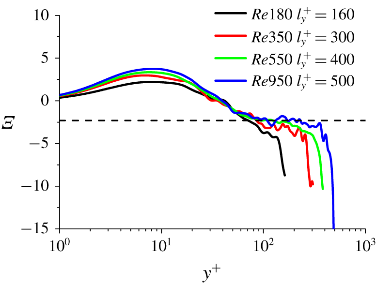
To assess the logarithmic scaling of the spanwise turbulence intensity, figure 16 shows the corresponding indicator function  $\unicode[STIX]{x1D6EF}$ of the second-order moment of the
 $w$-structures. It is readily noted that the plateau is observed in the range
 $80<y^{+}<250$ in Re950. It would be hypothesised that the logarithmic scaling of spanwise turbulence intensity is more significant at higher Reynolds numbers.
The variations of  $\unicode[STIX]{x1D6FE}_{1}$
,
 $\unicode[STIX]{x1D6FE}_{2}$ and
 $\unicode[STIX]{x1D6FE}_{3}$ as a function of
 $Re_{\unicode[STIX]{x1D70F}}$ for
 $AA_{w}$.

Wall-normal variations of the corresponding indicator function of the second-order moment for  $AA_{w}$ with selected
 $l_{y}^{+}$ for all cases.

4 Conclusions
In the present work, we adopted a three-dimensional clustering methodology to identify the wall-attached structures of streamwise and spanwise velocity fluctuations in turbulent channel flows at four Reynolds numbers ( $Re_{\unicode[STIX]{x1D70F}}=186$, 358, 547 and 934). The structures are further classified into high- and low-speed families, denoted by
 $PA$ and
 $NA$, respectively.
For the wall-attached  $u$-structures, our results show that the statistical properties of
 $PA_{u}$ and
 $NA_{u}$ are asymmetrical, and the former exhibit a closer resemblance to the theoretical predictions of the attached-eddy model, namely, (i) the spanwise length scales are self-similar with the distance to the wall (
 $y$), (ii) the population density is inversely proportional to
 $y$, (iii) the statistical moments obey a logarithmic wall-normal scaling and (iv) the inner peaks of the statistical moments increase as
 $\ln (l_{y}^{+})$. Although the low-Reynolds-number effect (
 $Re_{\unicode[STIX]{x1D70F}}=186$ and 358) obscures the geometric self-similarity, the logarithmic decay of the streamwise turbulence intensity carried by
 $PA_{u}$ is still maintained. Furthermore, we have provided an interpretation of the asymmetric behaviour between
 $PA_{u}$ and
 $NA_{u}$ from the perspective of sweep and ejection events:
 $PA_{u}$ are mostly associated with sweep events, while
 $NA_{u}$ are strongly correlated with the ejection events. As a result, the formation of
 $PA_{u}$ and
 $NA_{u}$ are different due to the asymmetry introduced by the wall:
 $PA_{u}$ are predominantly dominated by low shear flow from the upper domain of the boundary layer and
 $NA_{u}$ originate under the strong shear conditions of the near-wall region. For the wall-attached
 $w$-structures, no asymmetry is found between the high- and low-speed families, and their statistical properties are approximately consistent with the predictions of Townsend’s wall-attached model.
Note that the original attached-eddy model (Townsend Reference Townsend1976; Perry & Chong Reference Perry and Chong1982) and subsequent variants (Woodcock & Marusic Reference Woodcock and Marusic2015; Yang, Marusic & Meneveau Reference Yang, Marusic and Meneveau2016) are incapable of describing the asymmetrical features of high- and low-speed wall-attached  $u$-structures. The presence of attached eddies in the low-Reynolds-number wall turbulence presented here may aid the development of future investigations of the attached-eddy model and allow for computationally efficient strategies for wall-bounded turbulence prediction.
Acknowledgements
This work was funded by the National Natural Science Foundation of China (under grant nos 11772194 and 91952302) and the Coturb program of the European Research Council, and performed in part during the fourth Madrid Turbulence Workshop at UPM. We would like to thank Professor Jiménez for his kind invitation to the workshop. We also express our gratitude to the reviewers of this paper for their kind and constructive comments.
Declaration of interests
The authors report no conflict of interest.
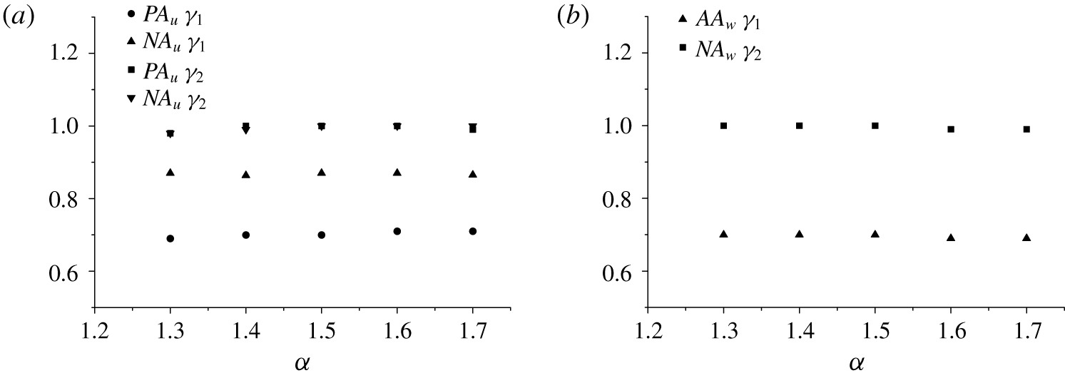
Appendix. Effects of the threshold $\unicode[STIX]{x1D6FC}$

The variations of  $\unicode[STIX]{x1D6FE}_{1}$ and
 $\unicode[STIX]{x1D6FE}_{2}$ as a function of
 $\unicode[STIX]{x1D6FC}$ for (a)
 $u$-structures and (b)
 $w$-structures in Re550.

The influence of the threshold  $\unicode[STIX]{x1D6FC}$ is examined. Figures 17(a) and 17(b) show the variations of
 $\unicode[STIX]{x1D6FE}_{1}$ and
 $\unicode[STIX]{x1D6FE}_{2}$ as a function of
 $\unicode[STIX]{x1D6FC}$ for the
 $u$-structures and
 $w$-structures in Re550, respectively. The indices barely change when
 $\unicode[STIX]{x1D6FC}$ varies from 1.3 to 1.7, indicating that the geometrical characteristics of the wall-attached structures are robust. Next, we examine the influence of
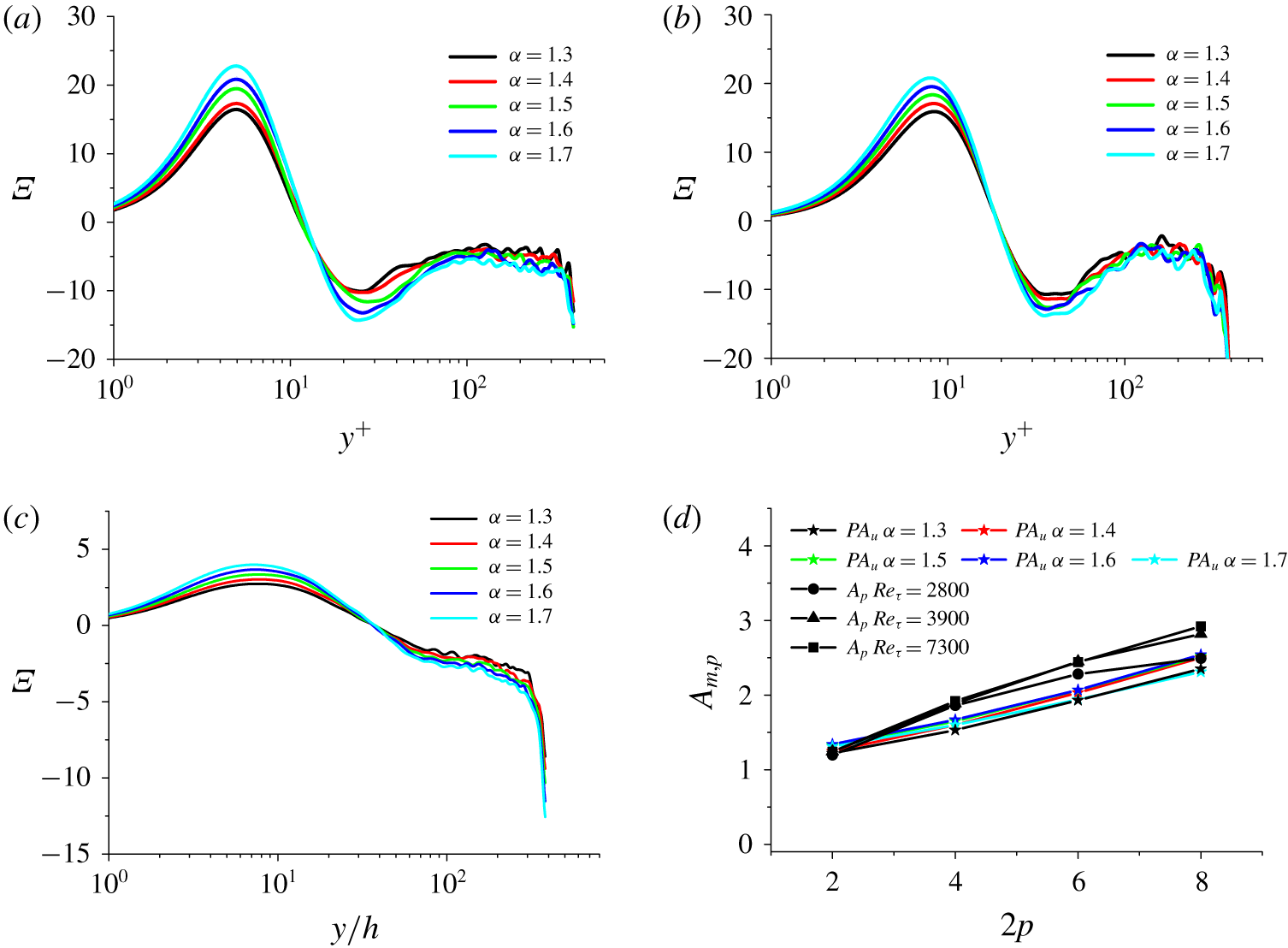
 $\unicode[STIX]{x1D6FC}$ on the statistical moments. For
 $PA_{u}$,
 $NA_{u}$ and
 $AA_{w}$, the indicator functions (
 $\unicode[STIX]{x1D6EF}$) of the second-order moment over
 $1.3\leqslant \unicode[STIX]{x1D6FC}\leqslant 1.7$ are shown in figures 18(a), 18(b) and 18(c), respectively. The results suggest that the wall-normal scalings of the second-order moment are independent of
 $\unicode[STIX]{x1D6FC}$. The growth rates of the inner peaks of
 $PA_{u}$ are plotted in figure 18(d) as a function of moment order
 $2p$ when
 $\unicode[STIX]{x1D6FC}$ varies from 1.3 to 1.7, and compared with the data obtained from high-Reynolds-number experiments (Meneveau & Marusic Reference Meneveau and Marusic2013). It can be seen that the growth rates of
 $PA_{u}$ do not change quantitatively within the range of
 $\unicode[STIX]{x1D6FC}$ considered.
The indicator functions of the second-order moment carried by (a)  $PA_{u}$, (b)
 $NA_{u}$ and (c)
 $AA_{w}$ with
 $l_{y}^{+}=400$ over
 $1.3\leqslant \unicode[STIX]{x1D6FC}\leqslant 1.7$ in Re550. (d) The growth rates of the inner peaks (
 $A_{m,p}$) of
 $PA_{u}$ as a function of the moment order
 $2p$ when
 $\unicode[STIX]{x1D6FC}$ varies from 1.3 to 1.7. The experimental measurements of
 $A_{p}$ are also shown for comparison (Meneveau & Marusic Reference Meneveau and Marusic2013).