1 Introduction
Finite-size or inertial particle dynamics are often encountered in nature and technological applications either in the form of bubbles or aerosols. Their motion differs markedly from infinitesimal particle dynamics as they exhibit clustering and dispersive behaviours, which are absent for infinitesimal fluid elements. Several studies (Tang et al. Reference Tang, Wen, Yang, Crowe, Chung and Troutt1992; Tio et al. Reference Tio, Linan, Lasheras and Ganan-Calvo1993; Martin & Meiburg Reference Martin and Meiburg1994; Vasiliev & Neishtadt Reference Vasiliev and Neishtadt1994; Marcu, Meiburg & Newton Reference Marcu, Meiburg and Newton1995; Crowe, Troutt & Chung Reference Crowe, Troutt and Chung1996) have analysed inertial particle dynamics in either analytically defined or numerically generated fluid flows. These studies are based on the Maxey–Riley (MR) equation (Maxey & Riley Reference Maxey and Riley1983), the equation of motion for small spherical particles in an unsteady non-uniform flow velocity field.
In Haller & Sapsis (Reference Haller and Sapsis2008) the authors performed a singular perturbation analysis of the MR equation and derived a slow manifold that governs the dynamics of sufficiently small particles. This low-dimensional manifold has the form of a modified velocity field, expressed in terms of the underlying flow velocity field and the particle parameters. The result is a reduced-order inertial equation that describes the particle kinematics. This analysis allows one to perform accurate time inversion, as the full MR equation becomes numerically unstable when integrated backwards due to its singular character. Moreover, due to the purely kinematic character, the inertial equation facilitates study of clustering properties (Sapsis & Haller Reference Sapsis and Haller2010) and the computation of attractive manifolds for finite-size particles (see Sapsis & Haller Reference Sapsis and Haller2009; Sapsis, Haller & Peng Reference Sapsis, Haller and Peng2010; Sudharsan, Brunton & Riley Reference Sudharsan, Brunton and Riley2016).
Despite the favourable properties of the inertial equation its use can be limited due to several reasons. First, the inertial equation is an asymptotic equation with respect to the particle size, and higher-order corrections require higher-order material derivatives of the flow field (Haller & Sapsis Reference Haller and Sapsis2008), which can be hard to obtain reliably, especially for experimental data. Even for smaller particles, the MR equation may not be valid, depending on the characteristics of the flow. In fact, for the case of neutrally buoyant particles, Sapsis et al. (Reference Sapsis, Ouellette, Gollub and Haller2011) revealed via a direct comparison with experiments that particles can have velocities different from those of the underlying flow field. Other studies (e.g. Daitche & Tél Reference Daitche and Tél2014) have suggested that the inclusion of the Basset–Boussinesq memory term can improve the performance of the MR equation, but in this case the derivation of a slow manifold approximation proves to be a formidable task.
Here we present a novel approach for the derivation of a kinematic equation for finite-size particles that relies on utilizing machine learning methods in combination with a basic physical model for the particle motion, in this case the standard MR equation. We employ the blended machine learning framework that was formulated in Wan et al. (Reference Wan, Vlachas, Koumoutsakos and Sapsis2018). The basic idea of this method is to machine learn the mismatch between data and an imperfect model that captures some of the underlying physics of the problem. Learning is performed using a long short-term memory (LSTM) recurrent neural network (RNN). The choice of an LSTM-RNN is important as it naturally incorporates memory into the resulting model. As a basic model for the underlying physics we use the first-order approximation of the slow manifold that is associated with the standard MR equation.
Note that while a purely data-driven approach using LSTM-RNN (e.g. Vlachas et al. Reference Vlachas, Byeon, Wan, Sapsis and Koumoutsakos2018) could have been employed, here we choose to maintain as much as possible of the underlying basic physics through the derived inertial equation from the MR model. This strategy has certain advantages, primarily related to the fact that the mismatch between the two models has much smaller variance and can be learned more efficiently. On the other hand learning the full model would require more data points and would ignore the MR equation, which may not be perfect but still captures some important aspects of the particle motion.
Therefore, in the present context, the combination of a basic physical model and a machine learning framework has the following favourable properties: (i) the resulting model is not limited by the particle size, as is the case in the asymptotic model – at least to the extent that finite-size particles are small enough that they can be described as points, (ii) we can directly employ data from experiments or high-fidelity DNS models, (iii) the model utilizes all the available physics for regions where data are not available, (iv) we have direct modelling of memory effects. We present our results for the case of spherical bubbles, but the extension of the analysis for aerosols is straightforward. Specifically, we train the blended model using data from the full (non-reduced) MR equation for a simple cellular flow. We then assess the learned model for different flows, a flow behind a cylinder and a two-dimensional turbulent flow, and compare the performance with the inertial equation. We perform this comparison both at the trajectory and the statistics level.
2 Kinematics of spherical particles
Let
 $\boldsymbol{u}(\boldsymbol{x},t)$
be the velocity field of a two-dimensional incompressible flow field of density
 $\unicode[STIX]{x1D70C}_{f}$
. We denote by
 $\boldsymbol{x}(t)$
the path of a finite-size particle of density
 $\unicode[STIX]{x1D70C}_{p}$
immersed in a fluid field with characteristic length
 $L$
. For spherical particles of radius
 $a\ll L$
, the Lagrangian particle velocity
 $\boldsymbol{v}(t)$
is assumed to satisfy the Maxey–Riley (MR) equation of motion (Maxey & Riley Reference Maxey and Riley1983; Haller & Sapsis Reference Haller and Sapsis2008):
 $$\begin{eqnarray}\displaystyle & \displaystyle \dot{\boldsymbol{x}}=\boldsymbol{v}, & \displaystyle\end{eqnarray}$$
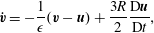 $$\begin{eqnarray}\displaystyle & \displaystyle \dot{\boldsymbol{v}}=-\frac{1}{\unicode[STIX]{x1D716}}(\boldsymbol{v}-\boldsymbol{u})+\frac{3R}{2}\frac{\text{D}\boldsymbol{u}}{\text{D}t}, & \displaystyle\end{eqnarray}$$
where
 $\text{D}/\text{D}t\equiv \unicode[STIX]{x2202}/\unicode[STIX]{x2202}t+\boldsymbol{u}\boldsymbol{\cdot }\unicode[STIX]{x1D735}$
denotes the material derivative and
 $\unicode[STIX]{x1D716}=1/\unicode[STIX]{x1D707}\ll 1$
with inertial parameter
 $\unicode[STIX]{x1D707}$
defined as
 $$\begin{eqnarray}\unicode[STIX]{x1D707}=\frac{R}{St},\quad R=\frac{2\unicode[STIX]{x1D70C}_{f}}{\unicode[STIX]{x1D70C}_{f}+2\unicode[STIX]{x1D70C}_{p}},\quad St=\frac{2}{9}\left(\frac{a}{L}\right)^{2}Re.\end{eqnarray}$$
Here
 $Re$
and
 $St$
denotes the Reynolds and particle Stokes number respectively. The density ratio
 $R$
distinguishes neutrally buoyant particles (
 $R=2/3$
) from aerosols (
 $R<2/3$
) and bubbles (
 $2/3<R<2$
). Note that the larger the inertia parameter
 $\unicode[STIX]{x1D707}$
, the less significant the effect of inertia; in the
 $\unicode[STIX]{x1D707}\rightarrow \infty$
limit, this equation describes the motion of a passive ideal tracer particle.
2.1 Slow manifold approach
For all
 $\unicode[STIX]{x1D716}>0$
, the MR equation (2.2) admits an invariant slow manifold (Haller & Sapsis Reference Haller and Sapsis2008) which has the asymptotic form
 $$\begin{eqnarray}M_{\unicode[STIX]{x1D716}}=\left\{(\boldsymbol{x},\boldsymbol{v})\boldsymbol{ : }\boldsymbol{v}\equiv \tilde{\boldsymbol{u}}(\boldsymbol{x},t)=\boldsymbol{u}(\boldsymbol{x},t)+\unicode[STIX]{x1D716}\left[\frac{3R}{2}-1\right]\frac{\text{D}\boldsymbol{u}}{\text{D}t}+O(\unicode[STIX]{x1D716}^{2})\right\}.\end{eqnarray}$$
Moreover, as shown in Sapsis & Haller (Reference Sapsis and Haller2008), although
 $M_{\unicode[STIX]{x1D716}}$
exists for all values of
 $\unicode[STIX]{x1D716}$
, it globally attracts all trajectories, in
 $O(\unicode[STIX]{x1D716})$
time, if and only if the following condition is satisfied:
 $$\begin{eqnarray}\unicode[STIX]{x1D706}_{min}[\unicode[STIX]{x1D64E}(\boldsymbol{x},t)+\unicode[STIX]{x1D707}\unicode[STIX]{x1D644}]>0,\quad \text{where }\unicode[STIX]{x1D64E}(\boldsymbol{x},t)=\frac{\unicode[STIX]{x1D735}\tilde{\boldsymbol{u}}_{\unicode[STIX]{x1D716}}(\boldsymbol{x},t)+\unicode[STIX]{x1D735}\tilde{\boldsymbol{u}}_{\unicode[STIX]{x1D716}}(\boldsymbol{x},t)^{\text{T}}}{2}.\end{eqnarray}$$
Here it is important to note that for a fixed
 $\unicode[STIX]{x1D716}$
, whether
 $M_{\unicode[STIX]{x1D716}}$
is globally attracting or not depends entirely on properties of the flow local to the particle and is unaffected by the velocity of the particle itself. Correspondingly, when a particle passes by a region where condition (2.5) is violated, its motion would diverge from
 $M_{\unicode[STIX]{x1D716}}$
, which repels all close-by trajectories.
Therefore, under the premise that (2.5) is satisfied along a particle trajectory and
 $M(t)$
is globally attracting for all
 $t>0$
, (2.4) provides an alternative description of the particle kinematics at all times. Keeping the leading-order terms, we obtain the inertial equation:
 $$\begin{eqnarray}\dot{\boldsymbol{x}}(t)\equiv \boldsymbol{v}^{\ast }(t)=\boldsymbol{u}(\boldsymbol{x},t)+\unicode[STIX]{x1D716}\left[\frac{3R}{2}-1\right]\frac{\text{D}\boldsymbol{u}}{\text{D}t}+O(\unicode[STIX]{x1D716}^{2}).\end{eqnarray}$$
Compared to the full MR equation (2.2), the inertial equation offers great modelling advantages as it has only half the dimension but non-zero divergence, which allows it to capture the clustering and dispersion of non-neutrally buoyant particles arising from finite-size effects. However, the accuracy of this approximation will be significantly compromised if (i)
 $\unicode[STIX]{x1D716}$
becomes larger and (ii) the local flow field is fast-changing either in space or time (
 $\boldsymbol{u}(\boldsymbol{x},t)$
has large partial derivatives). When either condition is satisfied, higher-order effects become non-negligible. Although closed-form analytical expressions for these high-order terms are available, they involve calculating high-order material derivatives which are difficult to obtain for arbitrary flow fields. Hence, we plan to utilize the first approximation of the inertial equation and combine this with available data in order to machine learn the higher-order corrections.
3 Blended slow manifold model
We aim to develop a new kinematic model blending the leading-order slow manifold approximation with a machine learning (ML) complement. The main purpose of the ML component is to identify when higher-order effects become important based on the local flow states encountered by the particle, and provide an accurate numerical estimate for the resulting kinematics. At the same time, this additional component does not raise the system dimensionality and keeps the model computationally efficient. More specifically, our proposed model follows the blended strategy in Wan et al. (Reference Wan, Vlachas, Koumoutsakos and Sapsis2018) and has the form
 $$\begin{eqnarray}\dot{\boldsymbol{x}}(t)=\underbrace{\boldsymbol{u}(\boldsymbol{x},t)+\unicode[STIX]{x1D716}\left(\frac{3R}{2}-1\right)\frac{\text{D}\boldsymbol{u}(\boldsymbol{x},t)}{\text{D}t}}_{\text{leading\text{-}order approx. }\boldsymbol{v}^{\ast }(t)}+\underbrace{G(\unicode[STIX]{x1D743}(t),\unicode[STIX]{x1D743}(t-\unicode[STIX]{x1D70F}),\unicode[STIX]{x1D743}(t-2\unicode[STIX]{x1D70F}),\ldots )}_{\text{data\text{-}driven model }\boldsymbol{v}_{d}(t)},\end{eqnarray}$$
which is a direct sum of the inertial model kinematics
 $\boldsymbol{v}^{\ast }$
and output of a data-driven model
 $\boldsymbol{v}_{d}$
. Here
 $\unicode[STIX]{x1D70F}$
is a time lag parameter and
 $\unicode[STIX]{x1D743}$
is a four-dimensional vector of flow states experienced by the particle along its own path at time
 $t$
:
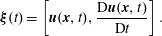 $$\begin{eqnarray}\unicode[STIX]{x1D743}(t)=\left[\boldsymbol{u}(\boldsymbol{x},t),\frac{\text{D}\boldsymbol{u}(\boldsymbol{x},t)}{\text{D}t}\right].\end{eqnarray}$$
These flow states are closely associated with the force exerted on the particle by the surrounding fluid. With the proposed model form, we aim to deduce the velocity of the particle from the forces it perceives by learning a data-driven function
 $G(\cdot )$
that maps the time series in
 $\unicode[STIX]{x1D743}$
to the corresponding series in
 $\boldsymbol{v}_{d}$
– velocity difference between the particle and the leading-order inertial model. Time history/delay coordinates are included in the model to compensate for the fact that
 $\unicode[STIX]{x1D743}(t)$
alone does not contain the full information required to evaluate the velocity on the slow manifold at time
 $t$
. Note that the choice for the components of
 $\unicode[STIX]{x1D743}$
is by no means unique and will likely affect the number of delays required for an accurate
 $G$
mapping.
We utilize RNNs as our learning method for
 $G$
. RNNs are a special type of neural network that provides a sequence-to-sequence mapping. The network reads input one at a time and computes the output from a running hidden state that is updated at every step based on the previous hidden state and the new input values, thus respecting the order of the input sequence. In particular, we utilize the LSTM (Hochreiter & Schmidhueber Reference Hochreiter and Schmidhueber1997), a special RNN unit, to map between discrete-time
 $\unicode[STIX]{x1D743}$
and
 $\boldsymbol{v}_{d}$
sequences. We use one LSTM layer with 128 hidden units, followed by one dense/fully connected layer with 64 hidden units and a rectified linear unit (ReLU) activation function to connect the input and output. The resulting model has a total of 76 032 degrees of freedom (DOFs).
The model DOFs are optimized with respect to the mean squared error loss on the output
 $\boldsymbol{v}_{d}$
. For our studies, training data are generated by directly integrating the original MR equation (2.2) and recording the model-required quantities (particle, flow velocities and material derivatives) along the path at some small uniform time step
 $\unicode[STIX]{x1D70F}$
. We treat these trajectories as the ground truth from which the model learns to predict the discrepancy between particle velocity and the leading-order manifold approximation. Predictions made in this way are single step because model output is not used to update the position of the particle and thus does not impact the model inputs in the future, regardless of any error made in the process.
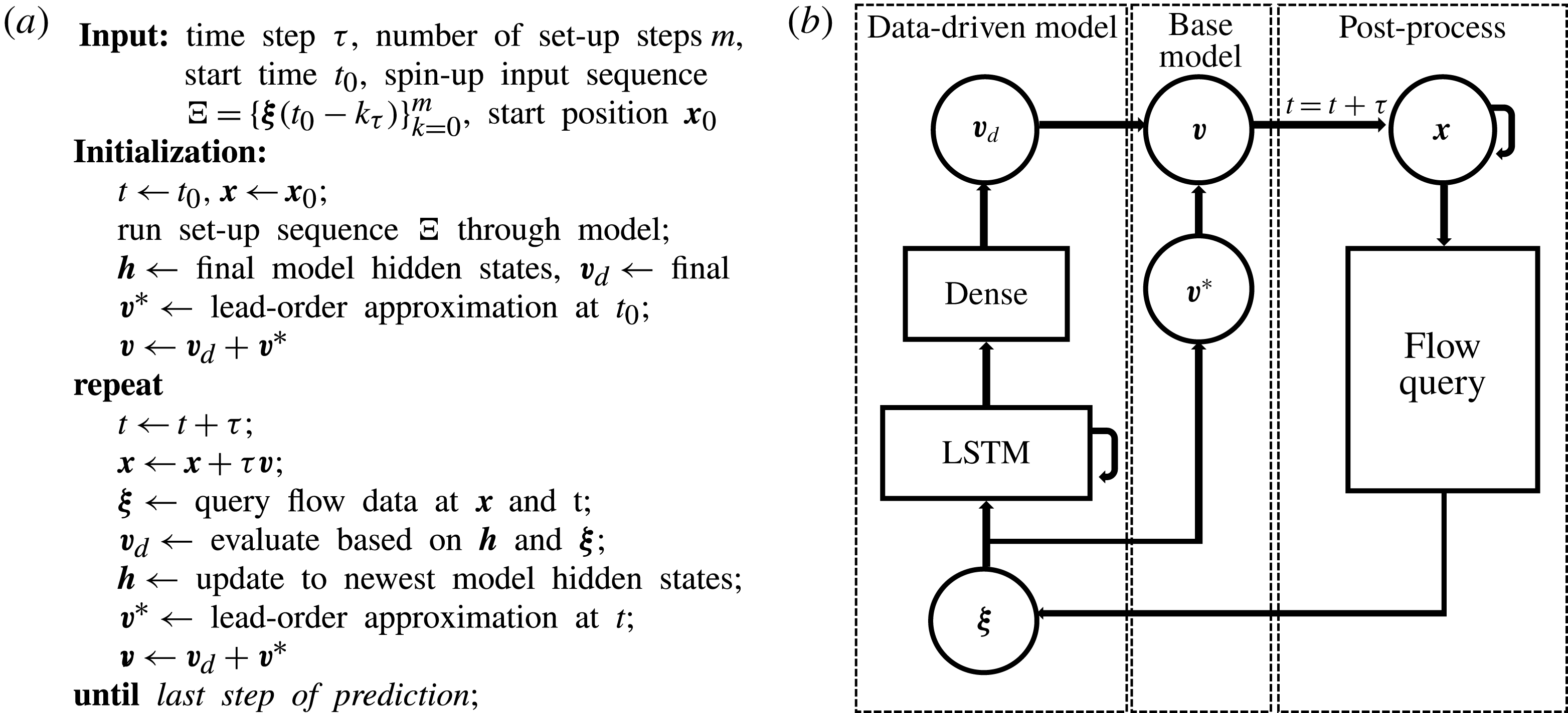
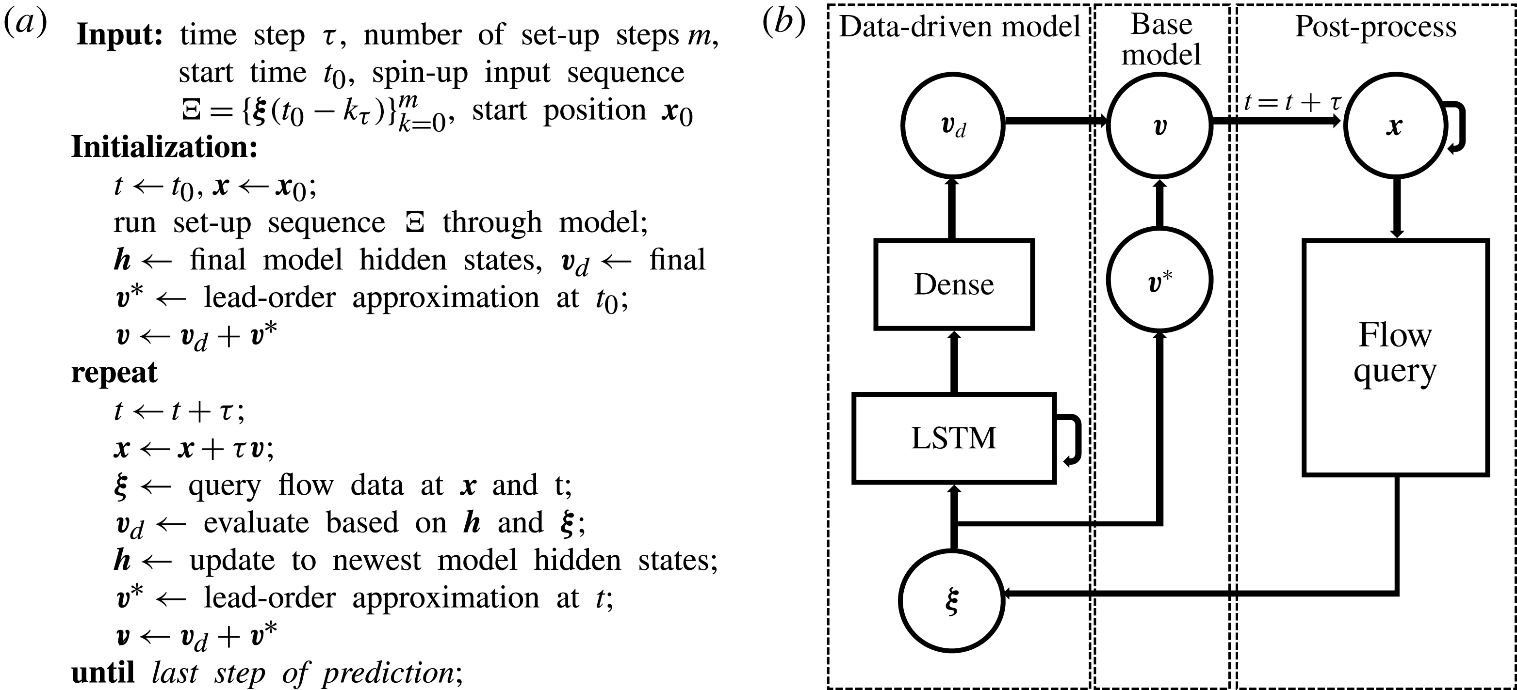
In a more practical prediction scenario, we often wish to forecast the trajectory of a particle for more than a single step. In this case, the predicted velocity fully dictates the particle position at the next time instant, which in turn determines the next model input. As a result, the model interacts with a flow database and queries for the next input based on the predicted particle position. Furthermore, an initial spin-up input sequence (typically of a few steps only) is needed such that zero initializations to the hidden states do not compromise performance. Figure 1 shows the overall multistep prediction algorithm with first-order time integration and the corresponding flow chart. We combine two such model instances, staggered in time, to achieve fourth-order integration accuracy. Finally, although it is possible to train the model by minimizing its multistep error (see Wan et al. Reference Wan, Vlachas, Koumoutsakos and Sapsis2018), we do not consider this option, mainly because the model would otherwise start to ‘anticipate’ future flow state based on training data, which is undesirable as we generalize the model to predict in time-dependent flows not encountered during training.
(a) Multistep trajectory prediction algorithm with first-order accurate time integration and (b) corresponding flow chart.
4 Applications
We demonstrate the proposed modelling methodology using three different flow problems. The first example consists of a simple two-dimensional flow with a simple periodic structure. We assume access to an excess amount of data (more than sufficient to accurately establish the functional approximation) and train the blended model to illustrate the main ideas of the proposed method. The second and third examples involve more complex flow structures – flow around a cylinder and turbulence in a periodic domain, respectively. We directly apply the models learned in the first example with no additional training and showcase the generalization capabilities of the proposed method to more realistic scenarios.
4.1 Cellular flow
We first consider the two-dimensional cellular flow model (Babiano et al. Reference Babiano, Cartwright, Piro and Provenzale2000; Cartwright et al. Reference Cartwright, Feudel, Károlyi, de Moura, Piro and Tél2010) representing a lattice of oscillating vortices or roll cells. The flow is defined by the stream function
 $$\begin{eqnarray}\unicode[STIX]{x1D713}(x,y,t)=A\cos (x+B\sin (\unicode[STIX]{x1D714}t))\cos (y)\end{eqnarray}$$
in the
 $x,y\in [-\unicode[STIX]{x03C0}/2,\unicode[STIX]{x03C0}/2]$
domain with periodic boundary conditions. The fluid velocity field can be derived by letting
 $\boldsymbol{u}=(-\unicode[STIX]{x1D713}_{y},\unicode[STIX]{x1D713}_{x})$
. Note that the time dependence in this flow can be suppressed by setting
 $B=0$
. Parameter
 $A$
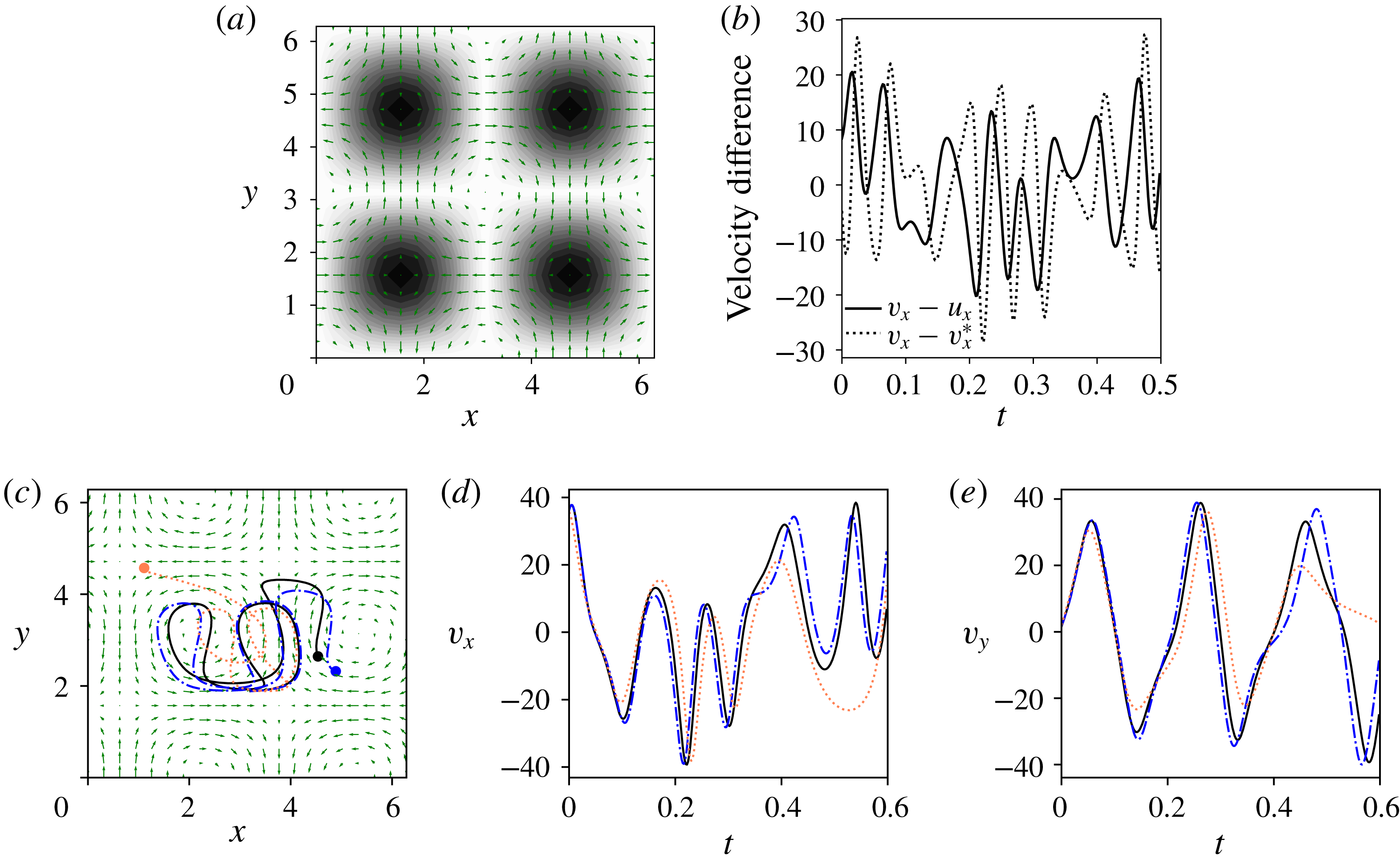
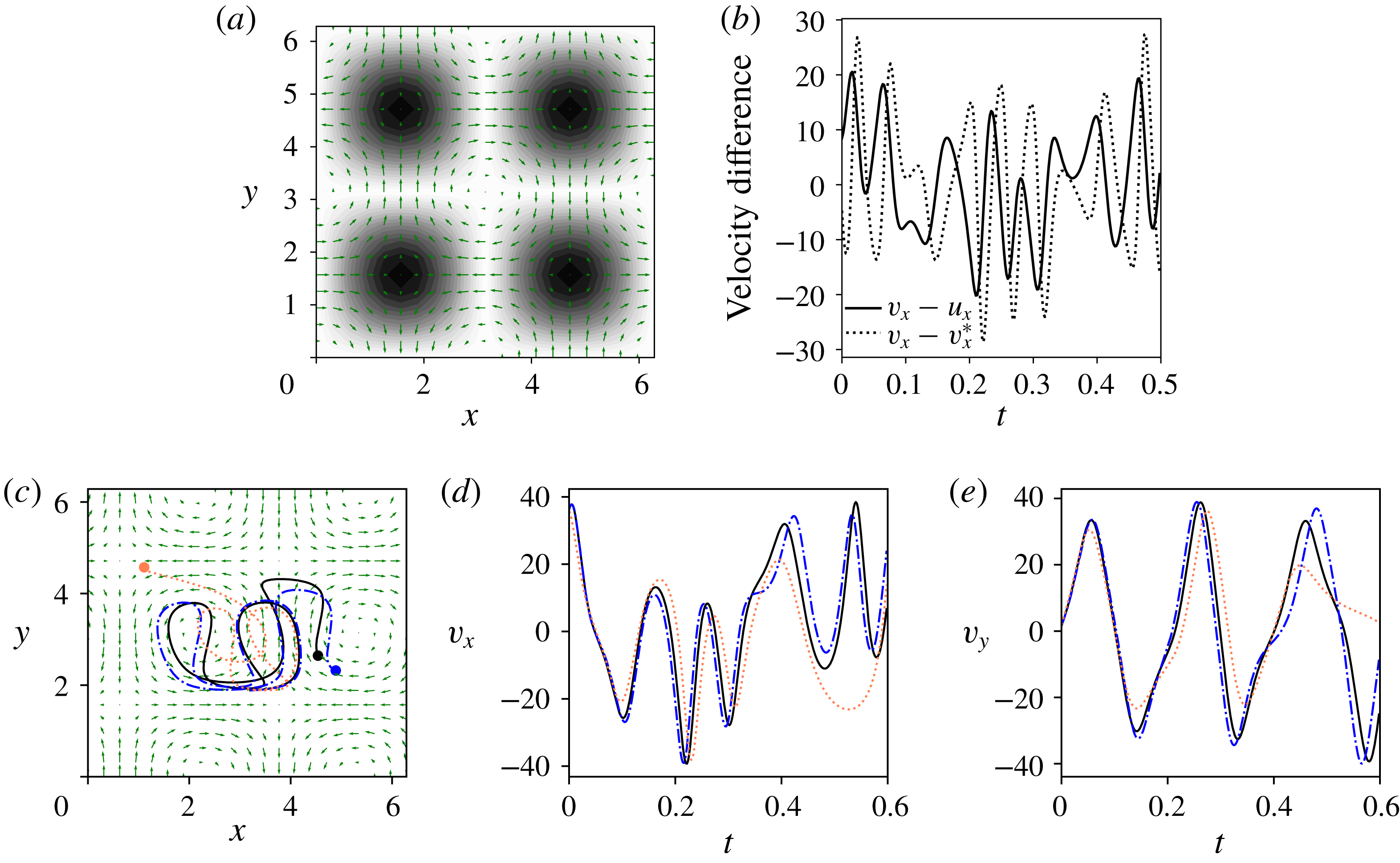
determines the strength of the vortices involved. Figure 2(a) shows the instantaneous velocity field at
 $t=0$
and contours of
 $\unicode[STIX]{x1D706}_{min}$
, the minimum eigenvalue defined in (2.5). Figure 2(b) shows the time series for the velocity difference between the particle and flow velocities, as well as between the particle and the leading-order approximation, of a bubble (
 $\unicode[STIX]{x1D716}=0.01,R=1.55$
) in a cellular flow with
 $A=47$
,
 $B=4.4$
and
 $\unicode[STIX]{x1D714}=11.5$
. These flow parameters result in large spatial and temporal derivatives in the velocity field, which leads to a large difference between the particle and flow velocities despite a small
 $\unicode[STIX]{x1D716}$
. In consequence, the effects of higher-order terms become prominent.
Cellular flow. (a) Velocity field at
 $t=0$
and magnitude of
 $\unicode[STIX]{x1D706}_{min}$
(background shading: lighter is higher
 $\unicode[STIX]{x1D706}_{min}$
). (b) Velocity difference between the particle and flow, and between the particle and leading-order approximation against time for a sample trajectory. (c–e) 300-step predictions made using the blended slow manifold model (— ⋅ —) and the leading-order approximation alone (
 $\cdots \cdots$
). (c) Trajectory in
 $(x,y)$
space (ending flow field shown in the background; solid circles mark the ending positions). (d,e) Predicted velocity time series in the
 $x$
and
 $y$
directions, respectively. Truth (——) from integration of (2.2) is plotted for comparison. Flow parameters are
 $A=32$
,
 $B=3.2$
and
 $\unicode[STIX]{x1D714}=9.2$
. Plotted trajectories start from
 $(x,y)=(3.20,1.88)$
at
 $t=0$
.
We apply the proposed method to learn a hybrid model for the slow manifold at fixed particle parameters
 $\unicode[STIX]{x1D716}=0.01$
and
 $R=1.55$
. Data are simulated by integrating (2.2) in cellular flow prescribed by (4.1) with random parameters drawn from uniform distributions:
 $A\sim {\mathcal{U}}[30,50]$
,
 $B\sim {\mathcal{U}}[0,5]$
and
 $\unicode[STIX]{x1D714}\sim {\mathcal{U}}[0,4\unicode[STIX]{x03C0}]$
. The randomization serves to inject more variety into the flow patterns seen by the model during training, and thus improve generalization. 1000 trajectories are generated at 1500 time steps of 0.002. 80% of the data are used for training and the remainder is divided equally for validation and testing. After 300 epochs, the model is able to achieve a single-step mean squared error (MSE) of
 $3\times 10^{-3}$
, averaged over all time steps and validation cases. This is almost perfect prediction, especially considering the fact that the leading-order approximation
 $\boldsymbol{v}^{\ast }$
has a MSE of 14.61 and the mean
 $L2$
-norm of
 $\boldsymbol{v}-\boldsymbol{u}$
is 25.18.
In figure 2(c–e) we compare the multistep prediction skill of the proposed RNN-blended model with the leading-order approximation
 $\boldsymbol{v}^{\ast }$
through an example test case. Due to much smaller single-step errors, the trajectory predicted by the blended model is able to remain close to the truth for a significant amount of time, despite being in a rapidly changing and unstable flow environment.
4.2 von Kármán vortex street
In a second example we consider particle motion in the von Kármán vortex street model first studied in Jung, Tél & Ziemniak (Reference Jung, Tél and Ziemniak1993). Finite-size particle motion in this flow has been studied in Benczik, Toroczkai & Tél (Reference Benczik, Toroczkai and Tél2002) and Haller & Sapsis (Reference Haller and Sapsis2008), who showed the existence of attractors for certain parameter values. The flow is governed by a stream function, and for simulation the system parameters are chosen such that the model approximates the Navier–Stokes solution for this geometry at
 $Re\approx 250$
with a flow period of
 $T_{c}=1.107$
.
We apply the model learned from the cellular flow trajectories in the previous example directly to the von Kármán vortex flow, since the learned slow manifold dynamics should be applicable regardless of the flow field encountered. In practice, we have found that this is indeed the case, demonstrating the robustness of the proposed approach. We have found that it is important to ensure that the model is never asked to extrapolate significantly, both in terms of the input and target. A rough way to check is to plot and compare the marginal density of each input and target dimension for training and test flows. For the trained model to perform well, regions where the test flow has non-negligible probability density should also have high density in the training flow.
For single-step predictions, we generate reference trajectories from (2.2) under the same particle parameters (
 $\unicode[STIX]{x1D716}=0.01,R=1.55$
) and time step (
 $0.002$
). These trajectories are randomly initiated in a rectangular box upstream of the cylinder:
 $x_{0}\sim {\mathcal{U}}[-2.1,-1.9]$
,
 $y_{0}\sim {\mathcal{U}}[-1,1]$
. The model is able to achieve a single-step MSE of 0.08, averaged over 50 test cases consisting of 550 time steps each. The performance is significantly better than the leading-order approximation alone, which records a MSE of 1.89 for the same data set. This result shows that the model we have obtained indeed generalizes well to new flow fields.
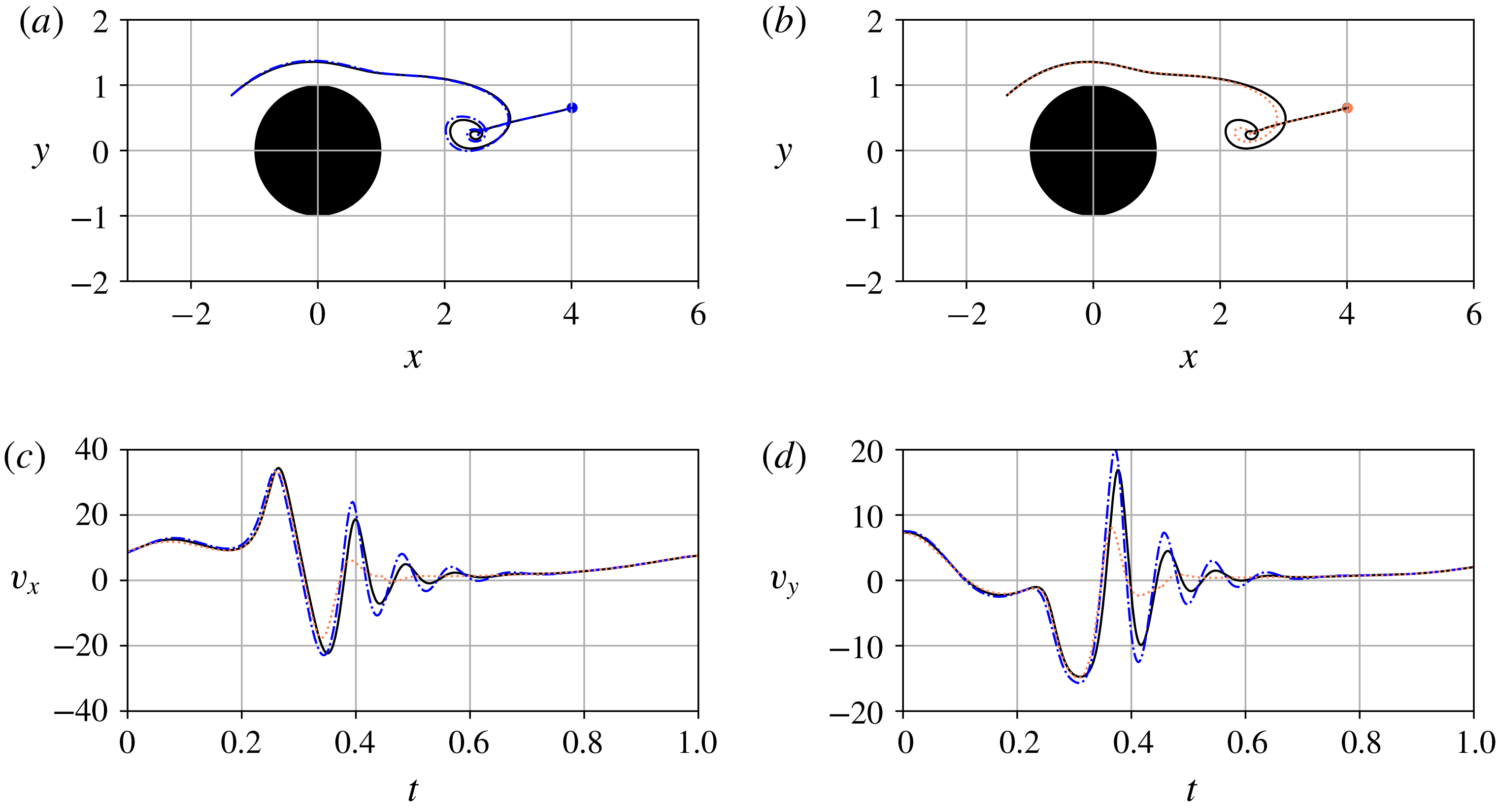
(a) 500-step trajectory predicted using the blended model for a von Kármán vortex flow trajectory compared with (b) the leading-order approximation. (c,d) Show predicted velocity versus time in the
 $x$
and
 $y$
directions. (Legend: truth ——; blended model — ⋅ —; leading-order slow manifold
 $\cdots \cdots$
).
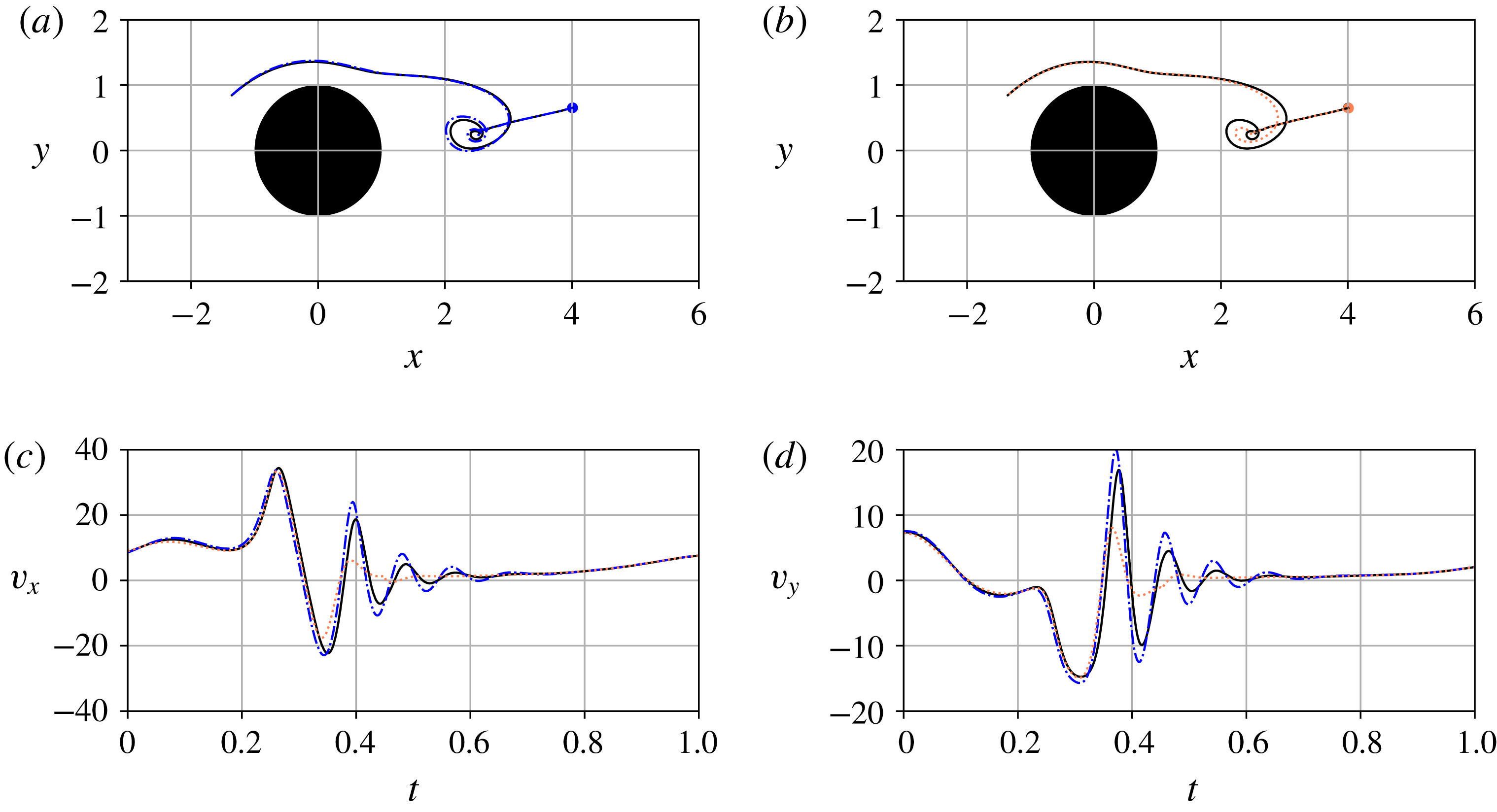
As for multistep predictions, we use a 50-step spin-up and predict for the 500 steps that immediately follow. Figure 3 shows an example prediction in terms of the resulting phase trajectory and velocity time series, compared with those given by the leading-order approximation. We observe that our blended model makes the biggest improvement in predicting how the particle travels with a shed vortex. It successfully captures the oscillation in the particle velocity as a result of the strong vorticity, which is not reflected in the leading-order approximations.
4.3 Two-dimensional turbulent flow
In the final application, we apply the blended model to an even more complex turbulent flow. The velocity field
 $\boldsymbol{u}$
for this flow is obtained as the numerical solution to the Navier–Stokes equation,
 $$\begin{eqnarray}\unicode[STIX]{x2202}_{t}\boldsymbol{u}+\boldsymbol{u}\boldsymbol{\cdot }\unicode[STIX]{x1D735}\boldsymbol{u}=-\unicode[STIX]{x1D735}p+\unicode[STIX]{x1D708}\unicode[STIX]{x0394}\boldsymbol{u}+\boldsymbol{f},\quad \unicode[STIX]{x1D735}\boldsymbol{\cdot }\boldsymbol{u}=0\end{eqnarray}$$
by a pseudo-spectral method with
 $128^{2}$
Fourier modes. We use an explicit Runge–Kutta method for temporal integration.
 $\unicode[STIX]{x1D708}=1/Re$
is the non-dimensional viscosity. The time-independent forcing
 $\boldsymbol{f}$
has constant amplitude
 $f_{a}$
and random phase, but only active for wavenumbers
 $\boldsymbol{k}$
on a circular ring, i.e. satisfying
 $k_{min}^{2}\leqslant |\boldsymbol{k}|^{2}<k_{max}^{2}$
, where
 $k_{min}$
and
 $k_{max}$
are the inner and outer radii respectively. Equation (4.2) is solved on a spatial domain
 $(x,y)\in [0,2\unicode[STIX]{x03C0}]\times [0,2\unicode[STIX]{x03C0}]$
prescribed with periodic boundary conditions. We choose to validate the blended model for flow parameters
 $Re=250$
,
 $f_{a}=1$
 $k_{min}=4$
and
 $k_{max}=5$
. Snapshots of the flow at the grid points are recorded every
 $2\times 10^{3}$
time units. A linear interpolation scheme is employed to compute the flow velocities between the grid points.
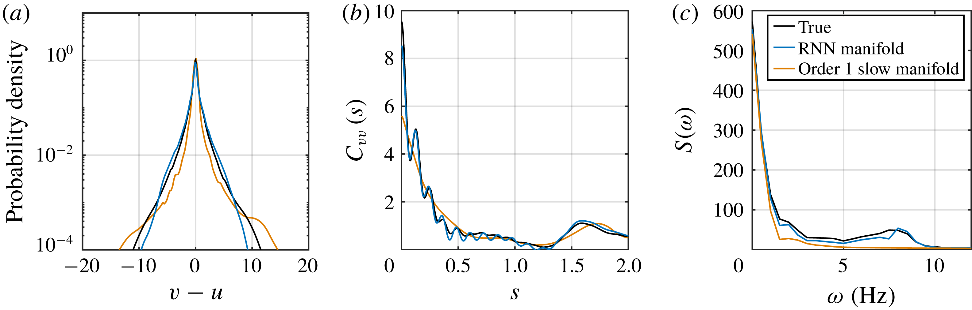
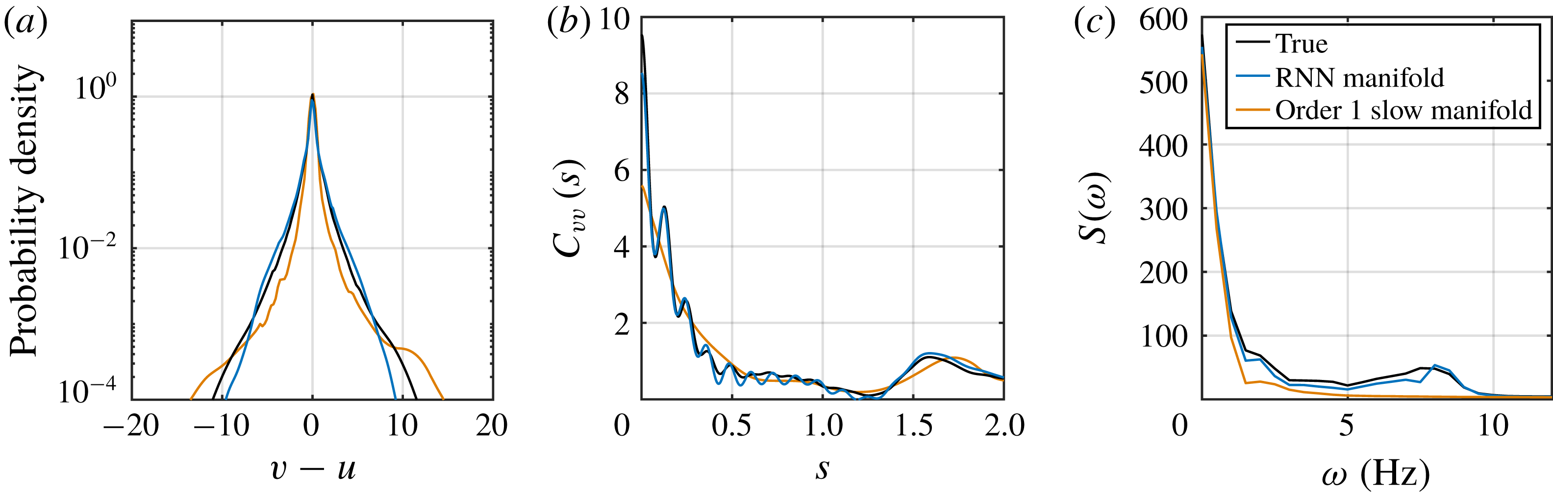
(a) Pdf for
 $v-u$
, i.e. the velocity difference between the particle and flow, (b) autocorrelation function and (c) power spectral density for
 $v$
as predicted by the true Maxey–Riley equation, multistep blended model and leading-order slow manifold approximations. Plotted quantities do not distinguish between
 $x$
and
 $y$
directions as the particle kinematics is roughly isotropic.
For this flow we model trajectories of particles with
 $\unicode[STIX]{x1D716}=0.05$
and
 $R=1.55$
. The particle inertia is increased from previous examples to raise higher-order effects. We train a model using data collected from the much simpler cellular flow with random coefficients:
 $A\sim {\mathcal{U}}[10,20]$
,
 $B\sim {\mathcal{U}}[0,3]$
and
 $\unicode[STIX]{x1D714}\sim {\mathcal{U}}[0,4\unicode[STIX]{x03C0}]$
. These parameters are slightly different from the values used in the previous examples to ensure the global attractiveness of the underlying slow manifold. After training, the blended model achieves a single-step prediction MSE of 0.09, averaged over 1200 steps and 1000 test trajectories randomly initialized in the spatial domain. In contrast, MSE of the leading-order slow manifold approximation is 9.88.
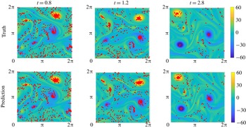
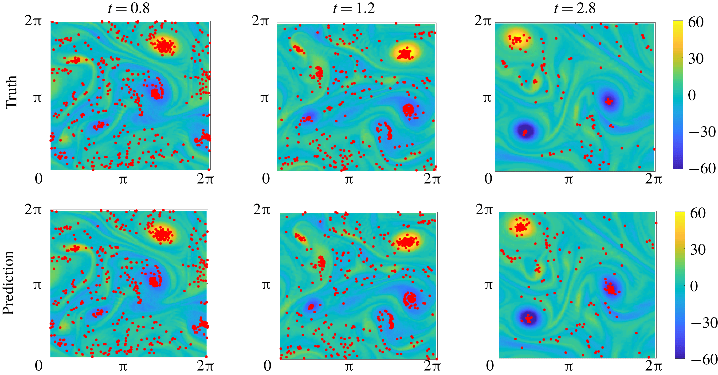
For multistep prediction we use a 200-step spin-up stage. Computing the multistep prediction error for this turbulent flow is not meaningful because any small errors made would grow exponentially with time due to the presence of chaos. However, we may still use the model to calculate long-time statistics. Running with 5000 realizations for 1000 steps, the empirical probability density function (pdf) of the difference between particle and flow velocities (in both directions, as the flow turbulence is isotropic) is shown in figure 4(a). We observe that the blended model provides a much more improved estimation compared to the leading-order approximation in both the bulk and tail regions. In figure 4(b,c) we compare the autocorrelation function and power spectral density estimations, respectively, for particle velocities. The blended model is better, primarily due to its ability to capture correlation patterns in the presence of vortices, although it tends to predict longer times for particles to be drawn to vortex centres and results in slightly stronger oscillation in the autocorrelation function. Figure 5 shows snapshots of the true and model-predicted particle positions at
 $t=0.8$
(end of spin-up period), 1.2 and 2.8, respectively. Similar characteristics are observed for both methods. In general, particles are drawn towards vortex centres because they are lighter than infinitesimal fluid elements (
 $R>2/3$
), as suggested by both the true MR and prediction models.
Particle position (marked by red dots) predicted by the Maxey–Riley equation (truth) and multistep blended model at time 0.8 (end of spin-up phase, zero error), 1.2 and 2.8, respectively. The flow vorticity field
 $\unicode[STIX]{x1D714}_{z}=\unicode[STIX]{x1D735}\times \boldsymbol{u}$
is shown in the background. Particles are drawn towards vortices. Distributions of their positions are captured to good accuracy.
5 Conclusions
We have developed a blended, model-based, machine learning approach for describing the motion of small spherical particles in fluid flows. The proposed method takes advantage of the existence of an analytical model: a low-dimensional, globally attracting slow manifold of the Maxey–Riley equation. It also employs delay coordinates through a machine learning strategy to complement the analytical leading-order approximation of the manifold and improve the overall accuracy. We have demonstrated the applicability through three different flow scenarios. We showed that a kinematical model constructed from particle trajectories in a flow with relatively simple structures can successfully generalize to more complex – and even turbulent – flows with no additional readjustment. The resulting single-step velocity predictions are significantly improved from the leading-order estimates. More impressively, the multistep implementation of the model is able to provide decent estimates for velocity statistics, as well as the autocorrelation and power spectrum. Our future endeavours will focus on the learning of the bubble dynamics directly from DNS simulations. In this case we expect that more variables will be utilized in the machine learning model, including the bubble size and fluid field pressure.
Acknowledgements
We thank Mr. A. T. Charalampopoulos for providing the code for the generation of the turbulent velocity fields in the third example. This work has been supported through the ONR MURI grant N00014-17-1-2676.