Introduction
Fuel cell components and microstructure
Fuel cells are efficient, reliable, zero-emission power generation devices for automotive applications that offer extended driving range and fast refueling. They are considered one of the most promising long-term solutions for cleaner vehicles. Among several types of fuel cells, proton exchange membrane fuel cells (PEMFCs) are considered to be the closest to widespread commercialization for automotive applications [Reference Kojima and Fukazawa1]. However, challenges remain with respect to their efficiency, durability, and cost. In a PEMFC, power is generated in membrane electrode assembly (MEA) that comprises of gas diffusion layers (GDL), including microporous layers (MPLs), and porous cathode and anode catalyst layers (CLs), separated by a dense, proton-conducting polymer membrane in the middle, as illustrated in Fig. 1. Each component of an MEA plays a crucial role in transport of species (electrons, protons, gases, and water) that support the electrochemical reactions in the CLs and the generation of power.
Schematic of a fuel cell with flow fields and MEA components: GDLs with microporous layers (MPL), anode electrode, cathode electrode, and membrane.

The microstructures in PEMFCs are heterogeneous in length scales that span over a few orders of magnitude. GDL, for example, is a few hundreds of micrometers thick carbon cloth or paper, made of carbon fibers with diameter range between 5 and 10 μm that are often coated with a nonuniformly distributed thin layer of hydrophobic polytetrafluoroethylene (PTFE) to help with water management. GDL serves as an interface between MEA and external current-collecting and gas-supplying flow field plates and provides electrical contact, thermal management, and reactant gas supply to and water removal from the CL [Reference Hoogers2, Reference Barbir3]. MPL, typically about 50- to 70-μm-thick layer coated on the GDL, is a mixture of electronically conductive carbon particles and hydrophobic PTFE binder. It provides pathway for the electrons, helps with thermal management, enables uniform gas diffusion, and maintains membrane humidification for improved performance [Reference Hoogers2, Reference Barbir3]. The most complicated aspect of species transport happens in the CLs. Both anode and cathode CLs, with thickness typically up to 10 μm, are comprised of a porous agglomerate network of carbon black nanoparticles (30–50 nm), metal catalyst, most commonly platinum (Pt), with particle size of 2–10 nm, and proton conductive polymer—ionomer (film thickness 2–8 nm [Reference More, Borup and Reeves4, Reference Lopez-Haro, Guétaz, Printemps, Morin, Escribano, Jouneau, Bayle-Guillemaud, Chandezon and Gebel5]). Carbon black, arranged in domains of connected agglomerates, provides percolation pathways for electron transport. At the same time, carbon black particles serve as a support for Pt catalyst for improved dispersion and enhanced surface area. Proton-conductive perfluorosulfonic acid (PFSA) ionomer, which is coating Pt/C agglomerates, works as a binder for carbon black and Pt, but more importantly, it provides transport pathways for protons between the reaction sites in the electrodes and the interface with the membrane. Ionomer can absorb water, which improves its proton conductivity, but complicates water management in the electrode. In addition, ionomer plays an important role in gas transport in the electrodes, since gases have to be transported through the ionomer film that often covers Pt reaction sites. Last but not least, pores within the electrodes transport reactant gases to and from the reaction sites and remove the produced water from the cathode.
The properties, composition, and microstructure of each component in the MEA affect the performance and durability of the fuel cell. Cathode CL plays an especially important role. Performance losses on the cathode are typically high due to the slower oxygen reduction kinetics and mass transport limitations caused by liquid water generated by the electrochemical reaction and carried to the cathode by electro-osmotic drag, impeding oxygen transport to the reaction sites. Cathode is also more prone to carbon corrosion in the presence of water under certain fuel cell operating conditions [Reference Enz, Dao, Messerschmidt and Scholta6]. Hence, a special focus is placed on the design of the microstructure and spatial distribution of components (carbon support, Pt catalyst, and ionomer) and pores in the cathode, and their effect on transport properties and effectiveness of the electrochemical reactions.
Current challenges in 3D imaging and modeling of fuel cell CLs
Mathematical modeling is often used to describe transport processes in CLs and contributes to understanding of parameters that affect its performance and degradation [Reference Secanell, Jarauta, Kosakian, Sabharwal and Zhou7, Reference Weber, Borup, Darling, Das, Dursch, Gu, Harvey, Kusoglu, Litster, Mench, Mukundan, Owejan, Pharoah, Secanell and Zenyuk8]. However, most macroscale transport models that are typically derived do not take into consideration actual CL microstructure and rather assume an ideal agglomerate model of the CL [Reference Weber, Borup, Darling, Das, Dursch, Gu, Harvey, Kusoglu, Litster, Mench, Mukundan, Owejan, Pharoah, Secanell and Zenyuk8, Reference Secanell, Karan, Suleman and Djilali9, Reference Cetinbas, Advani and Prasad10, Reference Epting and Litster11]. Full understanding of the effect of the microstructure on performance is hindered due to the complexity of the transport and electrochemical processes, large number of materials interacting across a wide range of length scales, and challenges to comprehend a realistic three-dimensional microstructure of the CL. With the advances in imaging techniques and computational power, 3D structural characterization coupled with modeling and simulation of transport properties and performance could open new avenues for better understandings of the MEA components microstructure and their effects on performance and durability of fuel cells. However, there are a number of challenges to overcome in both aspects of 3D imaging and modeling, especially over multiple length scales. Even though there is some reported work on utilization of 3D data sets in mathematical modeling of fuel cell properties and performance, they are very limited and do not span over multiple length scales and fuel cell components [Reference Weber, Borup, Darling, Das, Dursch, Gu, Harvey, Kusoglu, Litster, Mench, Mukundan, Owejan, Pharoah, Secanell and Zenyuk8, Reference Cetinbas, Ahluwalia, Kariuki, De Andrade, Fongalland, Smith, Sharman, Ferreira, Rasouli and Myers12, Reference Thiele, Fürstenhaupt, Banham, Hutzenlaub, Birss, Ziegler and Zengerle13, Reference Sabharwal, Pant, Putz, Susac, Jankovic and Secanell14].
Advanced 3D imaging techniques, such as electron tomography (ET), focused ion beam–scanning electron microscopy (FIB-SEM), nano- and microcomputed tomography (CT), have been utilized more recently to reveal actual CL microstructures [Reference Lopez-Haro, Guétaz, Printemps, Morin, Escribano, Jouneau, Bayle-Guillemaud, Chandezon and Gebel5, Reference Thiele, Fürstenhaupt, Banham, Hutzenlaub, Birss, Ziegler and Zengerle13, Reference Sabharwal, Pant, Putz, Susac, Jankovic and Secanell14, Reference Ziegler, Thiele and Zengerle15, Reference Epting, Gelb and Litster16, Reference Jankovic, Susac, Soboleva and Stumper17]. Imaging is typically completed only on one scale, missing the structural information on other scales. Nevertheless, these 3D data sets can be used for more realistic modeling approaches. However, use of 3D image data sets for modeling and simulation faces some common problems. On the image processing side, translating gray-scale image pixels to microstructure models that can be quantified and simulated can be difficult in several ways. First and foremost, accurate 3D reconstruction for ET, FIB-SEM, and nano-/micro-CT is often not straightforward. Image noise, most often not entirely avoidable, has to be removed, and contrast between features such as solid material and pore areas has to be enhanced. For 3D FIB-SEM, slices need to be accurately registered and subsequently reconstructed based on identifiable fiducials [Reference Sabharwal, Pant, Putz, Susac, Jankovic and Secanell14, Reference Ziegler, Thiele and Zengerle15]. For ET, beside image and tilt axis alignment, challenges arise from artifacts in the reconstructed images caused by limited number of tilt angles [Reference Leary, Midgley and Thomas18]. For nano-/micro-CT, beam hardening and ring artifacts are typical for heterogeneous material samples [Reference Boas and Fleischmann19].
After 3D reconstruction, the gray-scale data have to be segmented into separate material phases [Reference Sabharwal, Pant, Putz, Susac, Jankovic and Secanell14, Reference Salzer, Thiele, Zengerle and Schmidt20]. Manual and limited automated thresholding is typically applied, resulting in a time-consuming or sometimes even erroneous process (overestimation or underestimation of the segmented phase) [Reference Sabharwal, Pant, Putz, Susac, Jankovic and Secanell14]. The outcome of the image segmentation steps is a 3D material phase data set, where the voxel values denote the individual phases of the sample. For example, a processed FIB-SEM data set typically contains two material phases in PEMFC CLs, void and solid, while processed ET data set can contain more material phases, depending on the resolution and mode of operation (e.g., void, carbon, platinum, and still the most challenging ionomer phases). These data sets then can be analyzed using standard image quantification methods to obtain mathematical descriptors (surface areas, volume fractions, 2-point correlations, chord length, pore/particle/support size distributions, percolating volume fractions, tortuosity, etc.) of the material [Reference Secanell, Jarauta, Kosakian, Sabharwal and Zhou7].
Finally, effective transport properties can be deducted from the 3D data sets. One of the typically used approaches is that obtained mathematical descriptors can be used to indirectly determine an effective transport property, for example, by using a homogenization approach based on a simple random walk estimate [Reference Inoue, Yokoyama, Ooyama, Terao, Tokunaga, Kubo and Kawase21, Reference Inoue and Kawase22] or more complex distribution-based approaches [Reference Eikerling23]. The calculation of the effective transport properties based on the descriptors alone has the drawback as some structural assumptions have to be made. In comparison, an alternative approach would be to use voxels directly as mesh elements for numerical simulations [Reference Garboczi, Bentz and Martys24]. Generation of an explicit surface mesh, which is then converted into unstructured volume mesh, can be avoided. Furthermore, this methodology takes advantage of the hexahedron nature of the voxel elements and significantly reduces computational complexity and cost. This is the approach utilized in this work.
In this work, we are addressing a number of aforementioned challenges and providing a novel multiscale imaging and simulation approach that spans over three ranges of scales and fuel cell components. By utilizing advanced 3D imaging methods, improved segmentation approaches and direct image-based numerical calculations, we demonstrate, using effective electrical conductivity as an example, how this improved approach can be useful to provide important fuel cell structural parameters and advanced understanding of fuel cell properties and transport phenomena.
Results and discussion
Resolving microstructure on multiple scales
When a system with multiple length scales is investigated (e.g., from a few nanometers to hundreds of micrometers), both microscopy imaging and transport properties simulations need to be performed on several hierarchy levels and then appropriately combined. Using the imaging techniques mentioned earlier, microscopy data at three hierarchy levels were available and labeled as S1, S2, and S3 respectively:
(i) S1—nanoscale—obtained by ET (a few to hundreds of nanometers length scale)
(ii) S2—microscale—obtained by FIB-SEM (tens of micrometers) and,
(iii) S3—macroscale—obtained by 3DXRM (hundreds of micrometers)
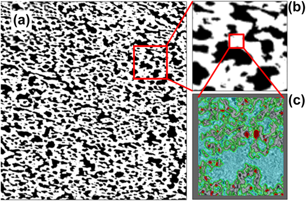
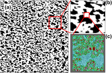
The length scale studied in this project spanned over a 5–6 orders of magnitude. The platinum particles were in the order of 3–10 nm, while the full thickness of the device was several hundreds of micrometers. It is important to note that only the smallest length scale S1 could distinguish between all the components of the CL: void, ionomer, carbon, and Pt. Each voxel could be assigned strictly to one phase without any ambiguity. Once the resolution was lowered with FIB-SEM, scale S2, each voxel in the solid phase within the CL becomes an unresolved mixture of the pore, carbon, ionomer, and platinum phases. Only solid and void (pores) phases could be resolved. Figure 2(a) shows a segmented FIB-SEM cross section of the cathode layer at the microscale S2. A magnification of a small section in Fig. 2(b) clearly shows the two segmented phases: pore ( $\Omega _{{\rm{pore}}}^{{\rm{S2}}}$) and multicomponent solid (
 $\Omega _{{\rm{eff}}}^{{\rm{S2}}}$). However the resolution of the FIB-SEM is not high enough to resolve the internal morphology and composition of the multicomponent solid (
 $\Omega _{{\rm{eff}}}^{{\rm{S2}}}$). Fortunately, the internal morphology and composition can be resolved by ET imaging at the nanoscale S1, Fig. 2(c). However, while the ET image provided the necessary resolution to resolve the platinum, carbon, and pore phase, it can cover a field of view that is only 1–2 μm in each direction. The data are not sufficiently large to model the physical properties of the CL with interconnected microscale porosity and carbon aggregates. To obtain larger sample volume, lower resolution has to be used by FIB-SEM. Imaging at even lower resolution at scale S3, using 3DXRM, enabled even larger field of view and sample volume, capturing MPL and details of the GDL layer in the MEA. However, the detection capability was lowered in the CL region, as each voxel was an unresolved combination of phases on scales S1 andS2. To resolve all phases, but also to capture large enough volume for analysis, a multiscale approach is necessary. Tables I and II list the segmented phases at the different imaged length scales S1 to S3, and the electrical conductivity parameters that can be simulated on these lengths scales.
Multiscale cathode layer as characterized by 3D imaging: (a) FIB-SEM segmented image, with the box indicating a small area magnified in (b). The white pixels denote the solid phase, whereas the black pixels represent the pore phase; (b) FIB-SEM segmented image zoomed in; (c) ET reconstructed area, with contour indicating fully resolved carbon (gray)/platinum (red)/pore (blue) phases. Ionomer (green) is artificially added as a 2-nm film.

Segmented phases at the different imaged length scales.

Description of the conducted electrical conductivity simulations on the lengths scales S1 to S3.

3D morphological analysis on multiple scales
The advantage of 3D imaging and volume reconstruction is the ability to analyze obtained 3D models and provide a number of structural parameters, some of which could be compared to other experimental values, while others are not possible to obtain otherwise.
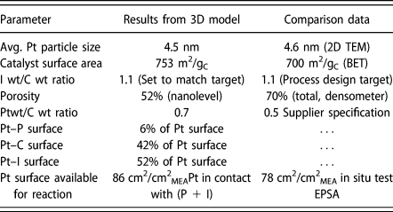
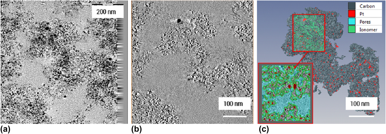
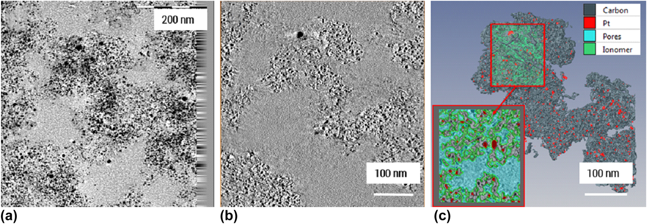
On the nanoscale, 3D model of the Pt/C agglomerate in the cathode CL obtained by ET provided an insight into the morphology of the agglomerates. Figure 2(c) shows segmented and reconstructed ROI region, where Pt particles are distinguished from a high-surface-area carbon support that has a complex morphology resembling wrinkled thin sheets. Pt is distributed mainly inside the wrinkles formed by the carbon sheets. Inner porosity of the agglomerate is therefore formed by these folded sheets, enabling gas access to active Pt sites through a maze of channels. PFSA ionomer distribution, as earlier mentioned, was challenging to determine; hence, ionomer was artificially introduced through the expand tool in Avizo (Thermo Fisher Scientific, Hillsboro, Oregon) as a 2-nm thin film covering whole Pt/C surface to fit the actual ionomer to carbon weight ratio (I/C). Scanning transmission electron microscopy with energy dispersive spectroscopy (STEM EDS) maps of the ionomer distribution using fluorine signal in the same region (Supplementary material) showed that ionomer is distributed throughout the agglomerate, confirming that this assumption is possibly close to reality. The 3D model on the nanolevel is of crucial importance for proper simulation of the transport properties, since the morphology of the carbon support and pore channels on the nanolevel is essential for electrical and gas transport. For example, electrical conductivity of the Pt/C agglomerates will be highly dependent on the electron percolation path and morphology of the carbon support in the agglomerates, as a main electronic conducive material. The closeness of the 3D model to the real agglomerate structure was assessed by comparing structural parameters obtained from the model and from actual catalyst measurements. Table III shows all structural parameters obtained from 3D model in comparison with available parameters from various experiments performed on catalyst powder (surface area by BET, Pt/C weight ratio), CL (total porosity by densometry [Reference Shukla, Stanier, Saha, Zahiri, Tam, Stumper and Secanell28]), and electrochemically measured electrochemically active Pt surface area (EPSA). Good agreement between 3D model and experimental values was achieved. For the Pt active surface area in the 3D model, it was assumed that all Pt surface in contact with pores and ionomer (Pt/(P + I)) is electrochemically active, while Pt surface in contact with carbon (Pt/C) does not participate in the electrochemical reaction. Hence, Pt/(P + I) from 3D model was compared to the experimental EPSA and comparable values were obtained. Somewhat higher value from the 3D model could indicate that not all Pt surface area is available for reaction in reality, due to Pt being buried in the pores or the agglomerate and not accessible to reactant gases. Somewhat higher Pt/C weight ratio could be explained by possibly higher content of Pt in this particular area. Porosity at the nanolevel of 52% involves only primary pores within the agglomerate and is lower than the total porosity obtained by densometry, which includes both primary and secondary porosity (pores between agglomerates). When combined with the obtained secondary porosity from FIB-SEM, a good agreement in total porosity was obtained, as explained later. Good agreement with the experimental values indicated that 3D model on the nanolevel can be used with a high confidence for further transport properties simulation. In addition, the 3D model provided structural parameters that could not be otherwise obtained, such as percentage of Pt in contact with carbon, ionomer, and pores. The morphological and compositional parameters obtained by 3DET in this work could be of high importance in mathematical models involving electrochemical reaction in addition to transport properties, and to the authors’ knowledge, such a comprehensive analysis has not been provided in the literature so far.
Morphological parameters obtained from the 3DET data set for cathode CL. Labeling: Pt = “Platinum,” P = “pore,” I =“ionomer,” C = “carbon,” EPSA = electrochemically active Pt surface area.

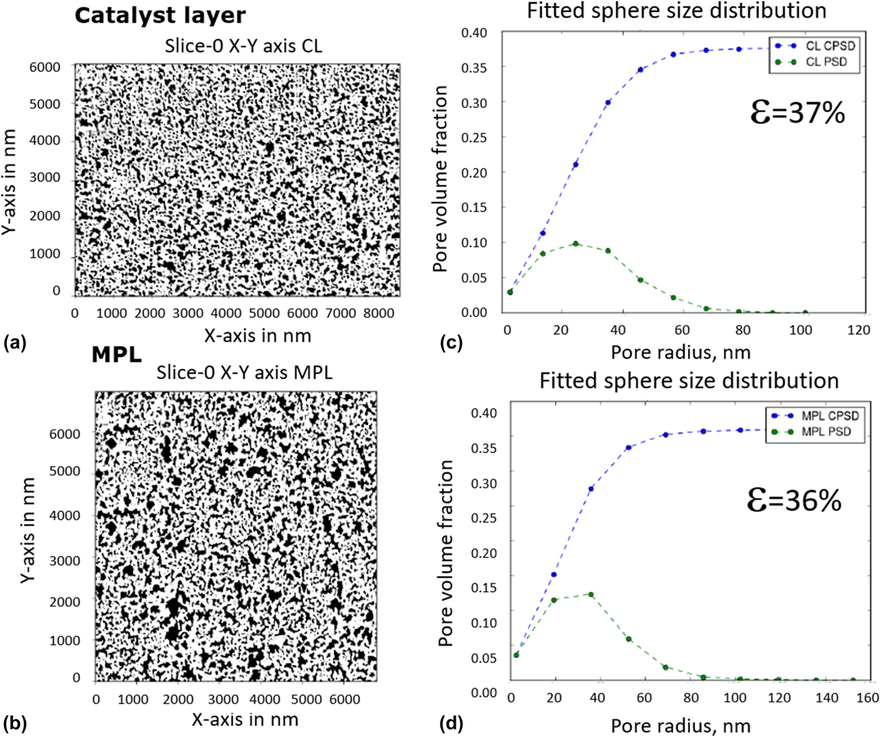
3D model analysis on the next length scale, S2, obtained by FIB-SEM provides valuable structural information on the void/solid distribution and secondary porosity in the CLs as well as MPL. Information obtained can be used to obtain effective transport properties, such as effective electrical conductivity in this work, on the microscale. Figure 3 shows the pore size distribution obtained by sphere fitting algorithm based on distance transform method [Reference Thiele, Fürstenhaupt, Banham, Hutzenlaub, Birss, Ziegler and Zengerle13] revealing similar distribution for CL and MPL, with MPL containing somewhat larger pores. Pore radius frequency for both layers peaks around 30–40 nm, and cumulative secondary porosity is close to 36–37%. Having in mind that the solid phase in FIB-SEM data set is constituted of Pt/C agglomerates similar to the one reconstructed on the nanolevel, which has 52% primary porosity, this would result in the overall CL porosity of 70% (0.37 + (1−0.37) × 0.52 = 0.70), which is in excellent agreement with the experimental value of 70% obtained by densometry [Reference Shukla, Stanier, Saha, Zahiri, Tam, Stumper and Secanell28].
FIB-SEM data sets and analysis results: segmented slices of the CL (a) and MPL (b); pore size distribution and total porosity for the CL (c) and MPL (d). CPSD: cumulative pore size distribution; PSD: pore size distribution.

Finally, the analysis of the GDL 3DXRM data sets revealed the morphology and fiber orientation on the macroscale. Porosity of the carbon paper from the 3D data set was 54%, which results in the total GDL/MPL porosity of 58% when combined with MPL porosity. Overall GDL/MPL porosity from the 3D model is somewhat lower when compared to experimentally measured porosity of 69% for used GDL/MPL by densometry. The difference could be coming from not fully resolved porosity of the MPL using FIB-SEM technique. The 3D model of the GDL can be further used to simulate effective electronic conductivity of the GDL.
After the structural analysis of the 3D data sets on three different length scales was completed and it was confirmed that the models satisfactorily represent the actual MEA, the next step was to proceed with the transport property simulations.
Multiscale simulation on images—effective electrical conductivity
It is well known how to calculate transport properties based on imaging data on any single hierarchy using commercial and open source simulation software packages [Reference Thiele, Fürstenhaupt, Banham, Hutzenlaub, Birss, Ziegler and Zengerle13, Reference Inoue and Kawase22]. However, the combination of all three image hierarchies into one unified, multiscale characterization framework of the effective transport properties has remained elusive. Two options are available: (i) Direct simulation can be conducted on the largest domain size on hierarchy S3, with sufficient resolution to fully resolve finer hierarchies S1 to S2. This requires enormous computational resources. (ii) Alternatively, direct simulation can be conducted on the largest domain size at S3. Although the voxel size at S3 is the coarsest, effective media theory is utilized to integrate physical properties computed at resolved scales S2 with higher resolution, which iteratively uses physical properties computed from S1. The generation of a computational domain suitable for such simulations has been demonstrated in the literature [Reference Thiele, Fürstenhaupt, Banham, Hutzenlaub, Birss, Ziegler and Zengerle13], but a transport simulation has not yet been executed. In this work, we are demonstrating the application of the second approach.
Direct numerical simulations were conducted on image voxels to compute physical transport properties [Reference Garboczi, Bentz and Martys24]. The physical property studied in this project is effective electrical conductivity. However, the multiscale approach is expected to be valid for other mechanical transport properties (e.g., diffusivity, thermal conductivity, permeability…).
The change in electrical potential ϕ through a simply connected domain Ω can be described by the continuity equation combined with Ohm’s law [Reference Bird, Warren and Lightfoot29],
 $$\nabla \cdot \left( {\sigma \nabla \phi } \right) = 0\;{\rm{on}}\;\Omega \quad ,$$
where σ is the electrical conductivity (scalar or 2nd-order tensor) and ∇ denotes the gradient operator. Two different potentials are applied along one of the three directions by specifying a high potential at the inlet face Γinlet and low potential at the parallel outlet face Γoutlet and no normal current at all other domain boundaries:
 $$\matrix{ \phi & \!\!\!\!= & \!\!\!\!{{\phi _{{\rm{inlet}}}} = 100} & \!\!{{\rm{on}}\;{\Gamma _{{\rm{inlet}}}}} \cr \phi & \!\!\!\!= & \!\!\!\!{{\phi _{{\rm{outlet}}}} = 1} & \!\!{{\rm{on}}\;{\Gamma _{{\rm{outlet}}}}} \cr {\left( {\sigma \nabla \phi } \right) \cdot n} & \!\!\!\!= & \!\!\!\!0 & \!\!{{\rm{on}}\;{\rm{all}}\;{\rm{other}}\;{\rm{boundaries}}} \cr} \quad .$$
The total current through the material can be calculated by integrating the normal flux component over either the inlet or outlet boundary, for example,
 $$\dot{N}_{\rm{e}}^{{\rm{outlet}}} = \int\limits_{{\Gamma _{{\rm{outlet}}}}} {\sigma \nabla \phi c \cdot n{\rm{d}}S} \quad ,$$
where n denotes the unit outward-facing normal vector and S boundary surface. In effective media theory [Reference Sabharwal, Pant, Putz, Susac, Jankovic and Secanell14, Reference Bird, Warren and Lightfoot29], the effective conductivity, c, for the potential ϕ through an equivalent homogenized domain Ωhom can be calculated by the simple one-dimensional solution of Eqs. (2)–(4):
 $${\phi _{{\rm{eff}}}} = \dot{N}_{\rm{e}}^{{\rm{outlet}}}{L \over {A\left( {{c_{{\rm{inlet}}}} - {c_{{\rm{outlet}}}}} \right)}}\quad ,$$
were A denotes the surface area of the inlet or outlet face and L the distance between them. To solve the partial differential Eq. (2) with the boundary condition (3), a finite element spatial discretization is directly built on the voxels of the segmented 3D imaging data, as opposed to using finite volume approach [Reference Sabharwal, Pant, Putz, Susac, Jankovic and Secanell14] or the reduction to a pore network model (PNM) [Reference Blunt30].
The calculation of the effective conductivity is carried out on scales S1 to S3. On scale S2 and S3, the bulk conductivity is replaced by the effective value on the previous scale. This approach is summarized in Table II.
Other physical properties that can be studied under this multiscale modeling framework include diffusivity, permeability, elastic modulus, and thermal conductivity [31].
Single-scale simulation results at the nanoscale S1
Simulation results on all scales and domains are presented in Table IV. On the nanoscale (S1), the effective electrical conductivity of the Pt/C agglomerate in the CL was simulated using 3D data set obtained by ET. The main conductive phase here was assumed to be carbon support, since Pt volumetric contribution to the electronically conductive solid is only 6%. The carbon bulk conductivity needed to calculate the effective agglomerate conductivity is not readily available. The value of 88.84 S/cm used in this study was taken from Secanell [Reference Secanell Gallart32], where it was estimated based on experimental conductivity data of packed Vulcan XC-72 carbon black [Reference Pantea, Darmstadt, Kaliaguine, Sümmchen and Roy33], a catalyst often used in fuel cell CLs. Effective conductivity expressed as percent conductivity of the pure conductive phase is given in the table in the in-plane (IP) direction X (parallel to CL) and through-plane (TP) direction Y (perpendicular to the CL). In-plane Z direction was not taken into account since the connectivity of the phases was questionable due to the artifacts of the segmentation. Comparable values in X and Y direction point out to the isotropy of the CL conductivity. The overall effective conductivity of the Pt/C agglomerates on the nanoscale was calculated by multiplying average (normalized) effective conductivity in % and bulk carbon conductivity. The obtained effective conductivity value for the Pt/C agglomerate of 4.31 S/cm is in agreement with the available literature values for Vulcan XC-72 Pt/C catalyst conductivities of 4 S/cm [Reference Pantea, Darmstadt, Kaliaguine, Sümmchen and Roy33, Reference Antolini34], as well as with our preliminary experimental values of 6 S/cm obtained for high surface area carbon (HSAC) catalyst compressed to 2MPa by four-probe measurement. A more detailed comparison with our experimental values will be published in an upcoming paper. CL pore space domain on scale S1, determined to take 52% of the Pt/C agglomerate volume, is considered to be fully nonconductive. In addition, ionomer was also assumed nonelectronically conductive.
Results of the multiscale simulation on 3D data sets.

Multiscale simulation results at the microscale S2
The length scale S2 is the first scale at which a multiscale approach is applied. The numerical simulation starts from 3D FIB-SEM data sets for the CL and MPL. As already stated, only solid and void phases can be distinguished without resolution of the inner solid structure on the nanoscale. The directional effective property values for both CL and MPL point out that the effective conductivities are mainly isotropic, with possible small anisotropy effect in through-plane Y direction (perpendicular to the CL and MPL). This could be a result of the compression during MEA fabrication. To calculate the overall effective conductivity of the CL and MPL, we assumed isotropy of both layers and averaged the directional effective conductivities.
To determine the overall effective conductivity of the CL, the multiscale approach was applied, where the information from the scale S1 was available and utilized. Namely, Pt/C agglomerate effective conductivity determined on the nanoscale S1 was used as a bulk (solid) conductivity on S2 scale. The obtained overall value for the effective conductivity of the CL was 1.5 S/cm. This value is in good agreement with the literature values that range between 1.0 and 2.0 S/cm for comparable CLs [Reference Du, Shi, Cheng and Yin35, Reference Suzuki, Murata, Hatanaka and Morimoto36], and also to our preliminary experimental values for in-plane conductivity of 1.7 S/cm obtained by four probe measurement. Since isotropy is assumed by both our approach and in the literature [Reference Suzuki, Murata, Hatanaka and Morimoto36], the values obtained by the simulation were considered acceptable.
MPL effective conductivity was computed from FIB-SEM single-scale model, by simple numerical simulation on S2 scale for single conductive (solid) phase, using bulk carbon conductivity, since no information on the nanoscale S1 was obtained. No literature or experimental values were available, since measuring of MPL electronic conductivity would require a stand-alone layer, which is not a straightforward approach. The closeness of the simulated effective conductivity will be assessed in combination with GDL in the next step of the multiscale simulation. Pores in both CLs and MPL were considered nonconductive and therefore not used in the current simulation case.
Multiscale simulation results at the microscale S3
The multiscale numerical simulation on the macroscale S3 starts with determination of the GDL effective conductivity using 3DXRM data, where carbon fiber and pore space in GDL are fully resolved. Effective conductivity for GDL substrate layer is first computed using single-scale model, where carbon fibers are the only conductive phase. The bulk fiber conductivity of 488 S/cm was used from Šafarova et al. [Reference Gregr and Šafarova37] for a similar type of fibers as in GDL used in this study. Due to the planar orientation of the GDL fibers, the in-plane (IP) conductivity of GDLs is typically higher than the through-plane (TP) conductivity [Reference Secanell Gallart32, Reference El-Kharouf, Mason, Brett and Pollet38, Reference Zhou and Liu39, Reference Mathias, Roth, Fleming and Lehnert40]. Hence, instead of single averaging of the directional conductivities previously used for isotopic MPL and CL, the in-plane conductivity in GDL was determined by computing a vector magnitude from X and Z directions,  ${\sigma _{{\rm{in\_plane\_normalized}}}} = \sqrt {\sigma _x^2 \times \sigma _z^2}$. The obtained value for in-plane conductivity is in good agreement with the literature data, as listed in Table IV. A higher through-plane conductivity of 44.3 S/cm obtained from our simulation compared to the literature values of 12–16 S/cm could be due to the stronger contact resistance effect in the through-plane direction, which was not accounted for in our simulation, and is affecting measured values in the literature.
Finally, multiscale simulation for the whole cathode side of the MEA was performed on 3DXRM data with three layers: GDL layer (with effective IP and TP conductivities computed from 3DXRM single-scale model), MPL layer (with effective conductivity computed from FIB-SEM single-scale model), and CL layer (with effective conductivity computed from FIB-SEM two-scale model, where carbon/platinum/nanoporosity aggregate phase conductivity is computed from ET data). In this step, all layers were modeled as homogenized layers, utilizing effective properties determined in the previous stages. In Table IV, we report effective conductivities for GDL/MPL layer and the overall GDL/MPL/CL combination obtained in this way. The in-plane GDL/MPL conductivity of 137.6 S/cm is comparable to the literature values for similar GDL/MPLs, while the through-plane values of 42.1 S/cm is higher, due to the contact resistance discussed earlier. It can be seen from the simulation that MPL does not affect GDL conductivity significantly, especially in the through-plane direction, since its MPL thickness is much smaller compared with GDL substrate thickness (∼30 um MPL, ∼230 um GDL substrate).
When the overall GDL/MPL/CL conductivity is calculated using the multiscale approach, the results showed that the in-plane conductivity is not significantly affected by the low-conducting CL, only 8% lower. However, the through-plane conductivity decreases from 42.1 S/cm for GDL/MPL to 16.95 S/cm for the whole electrode, almost 60% drop, due to the effect of the CL. Hence, to design MEAs with low ohmic resistance, our study confirms that one needs to focus both on CL and GDL/MPL design. Unfortunately, no literature or experimental data were available to compare our simulation results for the overall GDL/MPL/CL system, because experimental measurements of GDL/MPL/CL ohmic resistance in an assembled MEA are challenging to obtain. The same is true for the MPL layer. This, actually, proves the benefit of the reported approach, which enables understanding of separate and combined contributions of different components to the transport phenomena in the MEA. Such understanding could significantly help improve the design of the components and advance development of fuel cells.
Conclusion
A multiscale approach was utilized to image MEA cathode components using 3DET, FIB-SEM, and 3DXRM, followed by a direct numerical simulation of the effective electrical conductivity on obtained 3D data sets. The deduced structural and compositional parameters from the 3D data sets on the nano-, micro-, and macroscale had good agreement with the experimental data or specifications, proving that the models satisfactorily represented the actual MEA. 3D data sets were then used to proceed with the effective electrical conductivity simulations using the multiscale approach. The applied multiscale imaging and simulation approach provided effective electrical conductivity for Pt/C agglomerate, CL, and GDL/MPL, comparable to the experimental and literature values, while providing actual 3D morphological information on three length scales. Similar approach can be applied to determine other effective properties, such as thermal conductivity, diffusivity, and permeability. The accurate estimations of these properties, especially based on actual 3D morphologies, can be incorporated in the macroscopic fuel cell models to improve accuracy in predicting fuel cell performance. Effects of various Pt/C catalyst morphologies, CL, MPL, and GDL microstructures could be studied to design more efficient fuel cells.
Experimental section
Sample preparation
MEA for investigation was prepared in-house at Automotive Fuel Cell Cooperation Corp. (Vancouver, Canada) by conventional decal method. The catalyst ink slurry was made by dispersing catalyst (30 wt% Pt on high-surface-area carbon) with a mixture of ionomer solution, isopropyl alcohol, and DI water. The catalyst inks were coated on decal substrates using metering bars (Mayer bars) under a motorized draw-down table. Target Pt loadings for the cathode and the anode were 0.15 and 0.05 mgPt/cm2, respectively, and were measured on a dry decal by X-ray fluorescence. The weight ratio of the ionomer (dry basis) to carbon (I/C) was maintained at 1.1 for both cathode and anode. All effort was made to fabricate uniform electrodes, so that the multiscale imaging, which is rather local in nature, would be representative of the whole CL. The layer thickness uniformity was confirmed by SEM, and composition uniformity by scanning transmission electron microscopy with energy dispersive spectroscopy (STEM-EDS) (not shown here). The CLs were transferred onto commercially available Nafion membrane (NRE 211, DuPont™, Wilmington, Delaware) by hot-pressing to form the catalyst-coated membrane (CCM). MEA was assembled by hot-pressing the GDL onto the two sides of the CCM at 150 °C and 1.5 MPa pressure for 2.5 min.
Samples for ET and TEM imaging were prepared by embedding a small triangular piece of MEA (with GDLs removed) in TTE resin (trimethylolpropane triglycidyl ether and 4 4′-methylenebis 2-methylcyclohexylamine) (Sigma-Aldrich, Natick, Massachusetts), and microtomed to ∼100-nm thin sections using a Leica Ultracut UCT ultramicrotome (Leica Mikrosystem, Wien, Austria). The sections were deposited on 100-mesh Cu TEM grids.
A sample for the FIB-SEM analysis was cut from an MEA area positioned as close as possible to the TEM sample location. A small rectangular 1 × 2 cm MEA piece (including GDL and MPL) was cut with a sharp razor blade, sandwiched between two polished graphite blocks to keep them vertical, and placed in an SEM holder for cross-sectional analysis. Graphite blocks were tightened with a screw to allow sample stability and electrical connection with the rest of the holder.
For 3D X-ray microscopy (XRM) analysis, a small square piece (3 × 3 mm) of MEA, including GDL and MPL, was cut from an area close to previous two areas and wrapped in a transparent 3 M 467 MP adhesion tape. This X-ray transparent tape serves to hold the MEA layers together during 3DXRM analysis.
Obtaining 3D data sets
3D electron tomography (ET)
ET was utilized to image and reconstruct a Pt/C agglomerate in the cathode CL area at the smallest length scale S1—volume of approximate size 0.5 × 0.5 × 0.1 μm. ET was performed at 35,000 magnification in the bright-field mode using FEI Technai Osiris (Thermo Fisher Scientific, Hillsboro, Oregon) transmission electron microscope, with 200 kV acceleration voltage and Gatan Ultrascan 1000 XP-P CCD (Gatan Inc., Pleasanton, California) camera. A series of micrographs were recorded in a range of tilt angles from −60° to +70° at an interval of 1°. 3D volume was reconstructed using FEI Inspect 3D software (Thermo Fisher Scientific, Hillsboro, Oregon). The reconstructed 3D volume containing 385 orthoslices in xy plane, with voxel size 1.05 × 1.05 × 0.42 nm, was imported to Avizo software for image segmentation and 3D surface creation. Due to the complex nature of used carbon support and low gray-scale contrast with epoxy-filled pores and ionomer, no automatic image segmentation tools were helpful in segmentation of carbon. Consequently, carbon support was segmented manually using a brush tool in the Avizo Segmentation Editor. Pt particles were segmented using standard gray-scale threshold in the Avizo Segmentation Editor, selecting only gray-scale value of 0 (black) for Pt. Ionomer was challenging to segment from the tomography data sets due to the poor contrast difference with epoxy. Therefore, non-Pt and noncarbon areas were assigned to the pores, and ionomer layer was modeled as a 2-nm layer covering all Pt/C surfaces, with a total amount to match target ionomer-to-carbon weight (I/C) ratio of 1.1 [Figs. 4(a)–4(c)]. STEM-EDS maps of the same area confirmed that ionomer distribution resembles that of the 3D model. Once created, the 3D model of the CL area was analyzed using Avizo Surface Area Volume Module to determine surface areas and volumes, as well as contacts between all segmented phases, providing information to calculate a number of CL parameters, assuming known densities of carbon and ionomer [Reference Oberbroeckling, Dunwoody, Minteer and Leddy25] to be 2.00 g/cm2 and Pt to be 21.45 g/cm2. The model was validated by comparing selected parameters determined from the 3D model to the CL’s known specifications, such as BET surface area and Pt/C weight ratio of the used catalyst powder, CL Pt loading, electrochemical Pt surface area (EPSA), and layer porosity. In the case of a CL with uniform component distribution, which was used in our study, a good agreement between the model parameters and experimentally measured parameters or specifications was a confirmation that the reconstructed CL volume was representative of the whole CL. Finally, a representative region of interest (ROI) was selected for numerical simulation based on statistically sampled different subregions until surface area and Pt/C weight ratio reached a constant. In addition to ET, STEM-EDS mapping was performed in the same area, using Super-X EDX system with Silicon Drift Detector (SDD), to confirm the distribution of the CL components.
ET images and reconstruction of Pt/C agglomerate: (a) TEM image at 0 deg. tilt, after applied tilt correction and alignment; (b) one of the 385 reconstructed XY slices; (c) 3D model of the Pt/C agglomerate with the selected ROI.
Focused ion beam-scanning electron microscopy (FIB-SEM)
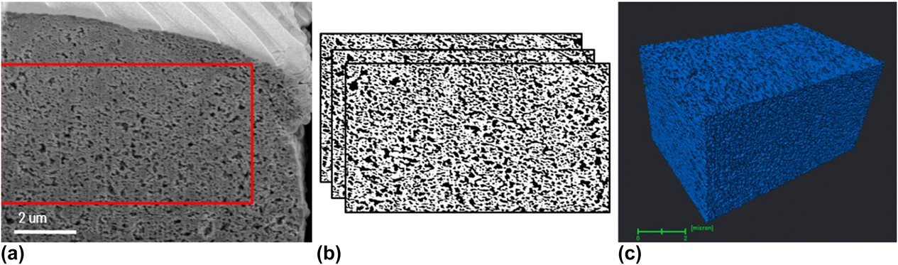
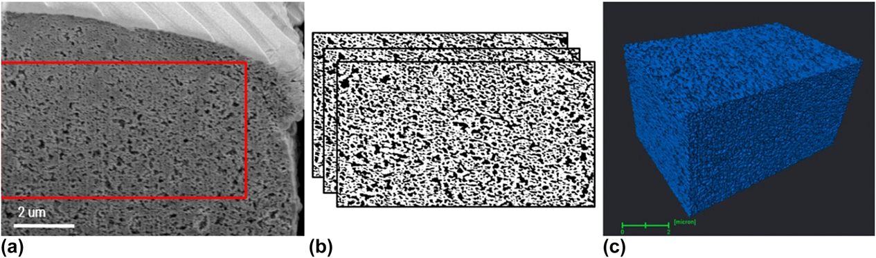
FIB-SEM imaging was performed to image and reconstruct a cathode catalyst volume on the next length scale S2—an approximate volume of 10 × 5 × 5 μm, pixel resolution 2.7 nm (Fig. 5). An FEI Helios NanoLab 650 (Thermo Fisher Scientific, Hillsboro, Oregon) dual beam system with a 30-keV Ga+ ion beam gun, operated at 3 × 10⁻⁶mbar chamber pressure was used for the FIB-SEM analysis. Once the CL ROI was identified from the sandwiched MEA, a Pt protective layer of ∼500 nm thickness was deposited using 83-pA ion current and 200-ns dwell time. On top of a protective layer, a set of line markers intended to help better image alignment were created at 45° tilt and 2-μm pitch using 83-pA ion beam current, 1000-μs dwell time, and 50% overlap. Following this process, one front and two side trenches were made around ROI using a 9.4-nA ion beam current to expose the region to be sectioned and minimize the possibility of material redeposition during slicing process. A smeared portion of CL cross section was then removed by applying 80-pA, 40-pA, and 24-pA beam currents sequentially, and a 24-pA current with 20 nm slice thickness was applied to perform slicing for a 3D reconstruction. High-resolution secondary electron microscopy (HRSEM) images with 4096 × 3536 pixel resolution were recorded after each slice using an in-lens TLD detector, 2 keV electron beam energy, immersion lens operating mode, 50 pA electron beam current. Image analysis including registration, filtering, segmentation, and binarization steps was performed using an improved in-house Python-based code as previously reported [Reference Sabharwal, Pant, Putz, Susac, Jankovic and Secanell14]. The improved image processing approach enabled more accurate reconstruction of the 3D FIB-SEM data and, hence, more accurate parameter quantification and property simulation in the next steps.
FIB-SEM images and reconstruction of cathode CL: (a) One of the raw FIB-SEM images; (b) segmented images with white areas representing solids and black areas representing voids; (c) 3D reconstructed CL with blue representing solids.
3DXRM
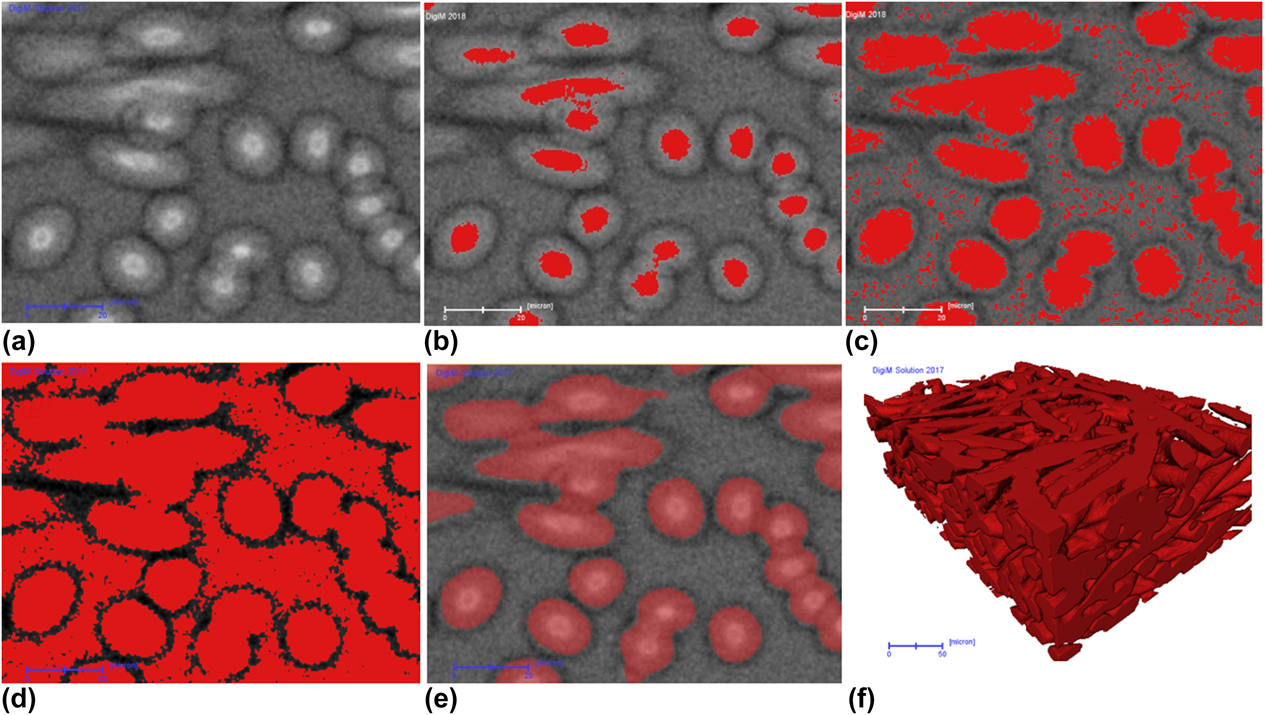
3DXRM was utilized to image the full MEA, including GDL, at the highest length scale S3—an approximate volume of 1000 × 1000 × 1000 μm. Zeiss Xradia Version 520 system (Carl Zeiss AG, Oberkochen, Germany) was used. The small square piece was mounted vertically on the rotation stage. Tomographic volume was reconstructed from 3000 projections using 80-kV energy, resulting in several different effective voxel sizes of 367 nm, 505 nm, 700 nm, 1.2 μm, 1.5 μm, and 3.2 μm. In 3DXRM, porous structure of GDL can be fully resolved. Other layers can be differentiated for upscaling purpose. Using a proprietary artificial-intelligence-based segmentation algorithm, robust and more accurate segmentation was obtained as illustrated in Fig. 6. This workflow, derived from random forest algorithm [26], starts with a set of seed voxels selected by the user to represent the pores and grains on a small, 2D training image. In addition to gray-scale intensity and its gradient, a basket of statistical measures was computed on the training data. Iterative refinement of the seed pixels on the small training image ensured that all important features were identified and correctly segmented. The segmentation procedure used on the training image was then automatically applied to the full 2D field of view and subsequently to the full 3D stack. To ensure accuracy, the number of statistical measures in the basket can be large. Furthermore, training images can be multiple 2D cross sections at different locations and orientations. Both considerations demand significant computing that desktop workstation cannot meet. A high-performance computing cluster was designed optimally for both such image processing and image-based numerical simulation [Reference Lezoray, Charrier, Cardot and Lefevre27]. Figure 6(a) shows a selected image used as the training image. Conventional single-threshold-based segmentation failed to segment the fiber material, as illustrated through Figs. 6(b)–6(d). When a low threshold value is used, the volume of the fiber material is significantly underestimated [Fig. 6(b)]. By increasing the threshold to the level indicated by Fig. 6(c), the volume of the fiber material is only slightly underestimated, but noise starts to build up on the porous region as the intensity fall-off toward the edge of the fiber is convoluted by the intensity of background voids. Smoothing will remove this noise, but the already underestimated fiber volume will be further reduced. More aggressive thresholding [Fig. 6(d)] will completely fail. In comparison, machine-learning-based segmentation algorithm was used utilizing the training image to iteratively refine the features, until a good segmentation is achieved [Fig. 6(e)]. The training set was then deployed to the full 3D volume to automatically segment the fibrous material.
Comparison of conventional thresholding-based segmentation and DigiM artificial-intelligence-based segmentation. (a) Original 3DXRM image. (b) Low threshold significantly undersegments fiber material. (c) Mild threshold that still undersegments fiber, but introduces noise. (d) Aggressive threshold that oversegments fiber. (e) DigiM artificial-intelligence-based segmentation on the training area. (f). Full 3D rendering of the final segmentation. Scale bar in (a–e) is 20 μm; scale bar in (f) is 50 μm.

Supplementary material
To view supplementary material for this article, please visit https://doi.org/10.1557/jmr.2018.458.
Acknowledgments
The authors would like to thank 4D Labs at the Simon Fraser University for access to the FIB-SEM and TEM instruments, as well as Ph.D. student Mayank Sabharwal at Prof. Marc Secanell Lab at the University of Alberta for processing FIB-SEM images. We are thankful to Dorina Manolescu from AFCC for CCM fabrication, Marcia Reid from McMaster University for microtome sample preparation and students Iva Jankovic, Brianna Bailey, and Moumita Saha for their tireless manual reconstruction of ET data set.