In 1933 President Franklin Roosevelt signed legislation creating the Tennessee Valley Authority (TVA), one of the world's first comprehensive watershed development projects. The TVA was created to construct a series of dams on the Tennessee River and its major tributaries. These dams were intended to improve flood control and navigation. As a byproduct, electricity was generated and distributed throughout the region. Electric rates, advertised by TVA, were among the lowest rates in the country. The low rates and TVA's commitment to extending service have historically been cited as a winning strategy for economic development in locations with abundant water resources.
The classic TVA story, as told by its champions, such as David Lilienthal (1944), describes how the agency both lowered electricity prices for existing customers and extended service to those without access from private companies. TVA's lower electricity prices reduced local firms’ input cost. Additionally, Lilienthal argued that the TVA expanded service to areas that had never been electrified. In both cases, lower power costs led to increases in productivity for those who gained new access. The TVA, thus, stimulated the local economies. This was particularly true for individuals and firms who sold their output in national and international markets. As the story is told, the TVA led to growth rather than transfers to the region.
Within a few short years, the TVA became the model intervention for any nation that sought to develop its water resources.Footnote 1 While the results discussed below are specific to the TVA, the fact that the TVA has served as a template for many development projects worldwide, should make it of interest for those studying other watershed development projects, and regionally targeted development projects more generally. Moreover, the rich data that is available to scholars of the TVA, allows us to carefully study its long, rich history and to fully examine the effects of this regionally targeted development project.
To explore whether TVA electrification boosted economic activity, I construct a county-level panel dataset for the southeastern United States from the 1930s through the 1950s. From 1933 to 1959 the TVA expanded its electric service territory, ultimately serving seven southeastern states. The growth was halted in 1959, when the TVA decided to become self-financing. The progressive expansion of TVA's electric service area allows us to study the short-run effects of regionally targeted development projects and improved access to electricity. There is an additional advantage because it is easy to disentangle the effects of the TVA from other programs in the region. Indeed, Department of Defense, Energy, and NASA spending in the region began in the late 1950s largely after the TVA's reach had stabilized.
I use within-county variation over time accounting for year-specific shocks in the state to measure TVA power contracts had on economic activity. Identifying the average treatment effect, however, is complicated by two matters; first, counties that contracted with the TVA were likely to have been the ones that would benefit from changing their electric provider, if these tended to be low income areas, the coefficient would be biased downward. Secondly, the TVA service area grew over time, so the timing of the switch between providers is likely driven by unobserved heterogeneity. I address these concerns in multiple ways; first, I impose sample restrictions limiting the sample to the region outlined in TVA's first power plans as its target service area, I include county-fixed effects to eliminate unobserved time invariant heterogeneity that may be correlated with selection, and I instrument for the TVA contract to address the timing of the switch in electric provider using the geographic distance between counties and newly constructed TVA dams. When new dams were completed, the cost of transmission fell. This type of variation over time serves as an exogenous cost shock. Both the locations and sequencing of the dams was determined by the U.S. Army Corps of Engineers (USACE) in 1930. At the very least, the instrument is uncorrelated with current economic conditions. Both the OLS and instrumental variables results suggest that the TVA did not have a statistically significant, positive or negative effect, on economic performance in terms of per capita retail sales, farm electrification rates, agricultural production, and manufacturing activity.
These results are in contrast to Patrick Kline and Enrico Moretti (Reference Kline and Moretti2013), henceforth KM, who find evidence that the TVA led to slight increases in median income and a shift from agricultural employment to employment in manufacturing. While my study does not focus on sectorial employment shares, our studies do overlap to some degree. Because median income is not available prior to 1950, I instead use retail sales per capita as a proxy, which is highly correlated with state level income figures. I also examine agricultural productivity and employment in manufacturing. None of these outcomes are strongly related statistically to the TVA's electricity program. There is some weak evidence that agriculture declined after switching to the TVA.
The differences between my study and KM arise for several reasons. First, KM examines the TVA over a 70-year period, beginning in 1940, whereas I examine the first 30 years of the TVA from its inception in 1933. KM's sample is composed of all counties in the United States weighted by their similarity to TVA counties prior to treatment. My sample is comprised of counties located in the Southeastern states as defined by TVA's target service area.
KM define treatment as all activity by the TVA, including dam construction, electricity programs, and reforestation programs, whereas my treatment variable only examines electricity contracts. Additionally, my identification strategy relies on the growth of the TVA service area over time, whereas KM define treatment as any county in the post1959 service area. It could be the case that dam construction leads to spillovers, such as those measured by Edson Severini (Reference Severini2012), while electrification does not. To ensure that my identification strategy is not driving the difference in results, I also estimate the effect of TVA electrification using matching methods similar to KM. When I estimate my model using matching methods, the estimates do not qualitatively change from the baseline OLS specifications. This indicates that TVA benefits probably came from something other than electrification.
Understanding the growth of the TVA service area, particularly from 1933–1939, is critical to evaluating the power program. In 1933 several municipally owned systems sought long-term power contracts with the TVA, likely leading to a negative selection bias (McCraw Reference McCraw1971). Secondly, the TVA sought a market within transmission distance of Wilson and Norris Dams, which led to the transfer of assets from private hands to the TVA. The negotiation of these acquisitions was complex and led to substantial increases in the TVA's service area. Because the TVA sought favorable test markets, failure to account for selection may lead to overly optimistic estimates of the TVA's power program.
The lack of statistical significance of the estimates makes it difficult to rule out the possibility of positive or negative effects associated with TVA electrification. To supplement the empirical exercise, I delve into the archival record of the TVA, the Federal Power Commission (FPC), the Rural Electrification Administration (REA), the National Electric Light Association (NELA), and the Edison Electric Institute (EEI). From these records, I reconstruct the average monthly bills paid by TVA residential consumers and compare them to the rates of private firms operating in the region. The data show that the rates charged by the TVA and private firms differed little; thus customers acquired by the TVA from private firms were unlikely to experience gains in productivity from lower input prices.
The TVA was also supposed to have expanded access to electricity. If the TVA connected customers that never had electric access, then it could have stimulated growth even if their prices were not lower. Using the records of the FPC, the REA, and the TVA, I show that all 101 municipalities that signed contracts with the TVA had had previous electric service. Of the 40 rural electric cooperatives that signed wholesale contracts with the TVA, only four did not receive loans from the REA for the construction of rural distribution lines (U.S. Department of Agriculture Rural Electrification Administration 1944). Combined, the lack of a price differential and TVA's weak record of extending access at the municipal level, suggests that the TVA simply transferred supply from private utilities to a federally owned wholesaler. If the TVA neither lowered prices nor heavily invested in distribution, it is difficult to attribute the growth in the region to the TVA's electric production. The complex interaction between production and distribution in electricity has echoes around the globe. Tania Barham, Mushfiq Mobrark, and Molly Lipscomb (2012), show that the expansion of hydroelectricity and distribution lines in Brazil raised economic activity and reduced poverty in part because these programs reached new customers. Similarly, Taryn Dinkelman (Reference Dinkelman2011) shows that electrification programs implemented after the end of Apartheid in South Africa, led to large productivity gains. These development programs resemble the REA far more than the TVA. Price Fishback and Carl Kitchens (Reference Fishback and Kitchens2013), show that the REA led to large increases in agricultural productivity and land values. The REA directly connected farmers to the grid. It also helped local cooperatives negotiate with utilities to sign wholesale contracts, or construct their own generation facilities. In light of this, the TVA is perhaps best represented as a new wholesaler in the region that assumed control of existing utilities service territory—a far less revolutionary role than hitherto assumed.
BACKGROUND ON THE TVA AND SOUTHERN ELECTRIFICATION
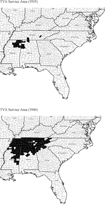
The TVA was created during Franklin Delano Roosevelt's first 100 days and charged developing the Tennessee watershed. This included flood control, navigation, soil reclamation, and electric generation and transmission. The TVA then built a series of dams on the Tennessee River and its major tributaries. While flood control and navigation were the official goals outlined in the charter, electricity generation and transmission became the focus of the agency by 1935. By 1952 the TVA provided electricity to 175 counties in seven southeastern states (See Figure 1).Footnote 2 The TVA relied on government appropriations to fund the construction of dams, reservoirs, power houses, and high voltage transmission lines, and to a lesser extent, distribution lines. Between 1933 and 1960 the TVA received over $20 billion in federal funding to cover these costs.Footnote 3
TVA SERVICE AREA

Initially, the TVA was tasked with disposing of excess electricity generated at Wilson Dam, which was transferred from the USACE to the TVA as a part of its charter.Footnote 4 Previously, the USACE contracted with private utilities in the region to distribute the excess powergenerated at the dam, which expired soon after the transfer of Wilson Dam. With the threat of an expiring contract, the TVA was faced with wasting surplus power, had no transmission capability, and had no market. After internal conflicts, the TVA pursued a plan of negotiating with private utilities and marketing its power directly to municipalities and cooperatives.Footnote 5 Government officials hoped that public power would be more efficient than private service. Thus the TVA experience would serve as a basis for comparison, or “yardstick,” both for future regulation of private utilities and further public power interventions. A key component of this baseline was establishing that the demand for electricity was highly elastic, in a hope to show that private utilities had been unfairly charging high rates. To achieve the “yardstick,” the TVA needed a market to serve under its new rate schedule. The TVA attempted to gain service territory by encouraging municipalities to vote in favor of municipal ownership so they would be able to contract directly with the TVA. The TVA signed its first wholesale electric contract with Tupelo, MS and began delivering power in 1934.
Additionally, the TVA encouraged municipalities to apply for grants and loans from the Public Works Administration (PWA) to construct duplicate distribution systems (Martin Reference Martin1953). This placed pressure on private utilities, such as Commonwealth and Southern (CS), which operated throughout the Southeast, to negotiate the transfer of service territory to avoid the devaluation of their assets (McCraw Reference McCraw1971). In 1934 CS agreed to transfer transmission and distribution assets to the TVA in 17 counties located in North Alabama, Northern Mississippi, and Western Tennessee within transmission distance of Wilson Dam, in exchange for territorial restrictions imposed on the TVA. The transfer of the Alabama and Tennessee properties was delayed by litigation until 1936.
Preferred stock shareholders in Alabama Power, a subsidiary of CS, filed a lawsuit challenging the legality of the government engaging in competition with private industry. In February of 1935 U.S. District Court Justice Grubb ruled that the TVA's power programs were unconstitutional: “Because there are generators at Wilson Dam, that doesn't give the TVA or United States government the right to sell as a private agency.”Footnote 6 His ruling, however, was overturned in the U.S. Supreme Court's Ashwander vs. TVA decision in 1936. The ruling set the precedent for a federally owned and operated corporation or agency to generate, distribute, and market electricity directly to customers from Wilson Dam, a narrow interpretation. It thus cleared the path for the TVA's expansion which had continued to sign new contracts during the litigation.
While the TVA was able to operate in the territory ceded by CS, its production capacity was exploding as its hydroelectric facilities were completed (e.g., in 1936 both Wheeler Dam and Norris Dam were completed). The TVA sought an enlarged test market with an industrial base; ultimately, it eyed the most valuable markets in Tennessee: Memphis, Knoxville, Nashville, and Chattanooga. One by one, each city voted to municipalize. This was troubling to the private companies, who relied on these large markets to cross subsidize thinner portions of their service territory. In each instance, the loss of the city corresponded to the sale of a wider operating area to include rural communities near the city. In the case of Chattanooga, then headquarters to the Tennessee Electric Power Company (TEPCO), another CS subsidiary serving most of Tennessee, the vote to municipalize led to the largest transfer of territory from private to public ownership. In 1936 TEPCO and 18 other utilities filed suit against the TVA, broadly challenging its constitutional legality in conjunction with the PWA. After an injunction in the lower courts and subsequent reversal, the U.S. Supreme Court dismissed the appeal in 1939, several of the 19 companies lacked standing. This settled any remaining challenges to the TVA's legal status as a power provider. Soon after the dismissal an agreement was reached between the TVA and TEPCO to transfer the entire system to the TVA for $78,000,000 (McCraw Reference McCraw1971). The deal increased TVA's service area to include the entire state of Tennessee, bringing it close to its TVA's configuration. With such a large increase in service territory, it was understood, on both sides, that the TVA would not have excess power to seek outside markets, thus the threat of expansion was temporarily alleviated.
As the TVA expanded its service territory, it marketed the many uses of electricity in the home and on the farm and used a promotional rate structure to attract customers. Table 1 compares TVA's 1933 rate schedule to Alabama Power's rural electric service rates in 1929. The TVA's rates were lower in the first block, and dropped faster than the Alabama Power rates as consumption increased. The lower rates made the TVA attractive to cooperative utilities and municipalities. Figure 2 shows the regional growth of the TVA between 1935 and 1940.Footnote 7 The low rates also suggest why locations served by the TVA could have experienced growth relative to locations not served by the TVA. Aggregate statistics, suggested that the TVA was improving the quality of life for its residents. Lilienthal claimed,“Per capita income had increased in the seven valley states 73 percent [in 1940] over the level of 1933; while for the same period the increase in the country as a whole was only 56 percent.”Footnote 8 Given the heavy presence of private power in the region prior to the formation of the TVA, and the transfers from private hands to the TVA, the aggregate statistics cannot reveal the TVA's true impact. In particular, the observed growth in output could simply reflect the South's recovery from the Depression.
ALABAMA POWER RURAL ELECTRIC RATE 1929 AND TVA SCHEDULE 1933

Sources:
Alabama Power Rural Rate Schedule Edison Electric Institute: “Developing Electric Service for the Farm as Exemplified by the Organizations and Methods of Alabama Power Company Serial Report of the Rural Electric Service Committee,” 1929. TVA Rate Schedule reported in the 1934 TVA Annual Report.
SAMPLE CONSTRUCTION
The data I use come from a variety of primary sources. Per capita retail sales, the farm electrification rate, value of farm products per farm, the value of farmland and equipment per farm, manufacturing value added, and number of manufacturing workers all come from census and governmental reports collected by Michael Haines (Reference Haines2004), as well as more recent efforts by Fishback, Haines, and Paul Rhode (Reference Fishback, Haines and Rhode2012) to digitize the county reports of the 1940 census of agriculture. The census provides county farm electrification rates in 1930, 1940, 1945, 1950, and 1954. Farm product values and the value of farm land and farm capital are available in 1930, 1940, and 1950. Retail sales were reported in 1929, 1933, 1936, 1939, 1948, and 1954. Per capita measures were then constructed by interpolating the population between census years. Manufacturing value added and the number of manufacturing employees were reported in 1929, 1931, 1933, 1935, 1937, 1939, 1947, and 1954. All nominal dollar values were adjusted to 2009 values using the CPI.
TVA SERVICE AREA GROWTH, 1930–1952

The TVA report,“Rate Reductions by the Distributors of TVA Power” reports when each distributor signed a wholesale electricity contract with the TVA. The locations of each cooperative service area were then obtained through each state's rural electric cooperative association's maps. A county is determined to be served by TVA in a given year if at least one municipality or a cooperative utility serving in the county had a power contract with the TVA.
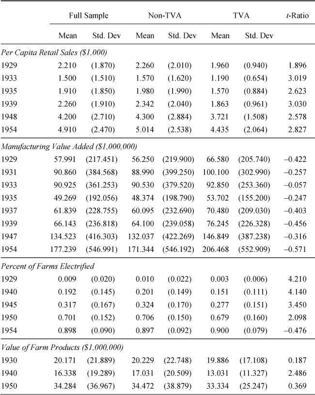
The primary sample used in the estimation was restricted to include counties in the southeastern United States: Alabama, Arkansas, Florida, Georgia, Kentucky, Louisiana, North Carolina, South Carolina, Tennessee, Virginia, and West Virginia.Footnote 9 In order to form a balanced panel, I further restrict the sample to include counties having no more than 1 missing observation for the given outcome of interest.Footnote 10 Table 2a reports summary statistics for all counties, columns 2 and 3 present the mean and standard deviation for counties that never joined the TVA, while columns 4 and 5 present the summary statistics for counties that ultimately became a part of the TVA by the end of the sample period. Column 6 presents t-statistics from difference in means test between TVA and non-TVA counties.
Table 2b shows that counties that were a part of the TVA and those that were not had been quite different. Counties that were served by the TVA were poorer than the other counties in the sample. Per capita retail sales were typically only 80–90 percent of per capita retail sales in the surrounding areas in 1929 and 1933 prior to the TVA and these differences persisted over time. TVA counties also had lower farm electrification rates. Agricultural production tended to be similar in 1930, however by 1940 there were significant differences. By 1950 differences in agricultural production were insignificant between TVA and non-TVA counties. Neither counties receiving electricity from the TVA or an alternative source had large differences in the manufacturing value added (it was low everywhere). The raw data make it clear that there was substantial growth in the Southeast United States over time and significant variation in all of the outcome variables across space. From 1930 to 1960 retail activity more than doubled, electrification reached almost every farm, farm productivity increased over 50 percent, and manufacturing tripled. Initially at least, it is unclear wither these increases would have occurred without the TVA, or if the TVA led to faster growth that closed the initial gap.
SUMMARY STATISTICS

Note:
Retail Sales per Capita are summarized in $1,000s, however the estimation below will use the actual dollar value.
Source:
Haines (Reference Haines2004).
EMPIRICAL STRATEGY
The statistics above indicate that there is substantial county-level variation over time and place. I use this variation and the timing of TVA electric contracts to identify how the TVA changed economic outcomesoutlined previously. If TVA electricity contracts were randomlyassigned, their average impact could be estimated with the following ordinary least squares regression:

Where Yit is the outcome of interest. is equal to one for every county with at least one distributor under contract with the TVA in that year, therefore, α1 would then be interpreted as the average treatment effect of a TVA power contract on the given outcome. However, the power contracts were not randomly signed, municipalities that believed they would benefit by contracting with the TVA and places that the TVA viewed as ideal test markets became the core of TVA's territory.
Thus selection would bias these naive estimates. I address this selection in multiple ways. First, I include county-specific fixed effects δi, to eliminate unobserved heterogeneity arising from time invariant features at the county level. I further control for unobserved shocks that occur nationally, such as growth associated with the end of the Depression by the including year-fixed effects, γ t . Unobserved shocks at the state level that change over time, such as changes in state legislation, are captured by the inclusion of state-year fixed effects, γ t λ s . I identify the effect of the TVA's power contracts by using variation within a county over time while controlling for year-specific shocks at the state level to determine if outcomes improved within counties following a switch to the TVA. I also include a variety of controls measured prior to treatment, X i,1930, interacted with the year-fixed effect, to control for other differences within the county that may not be captured by the inclusion of the county-fixed effects.
The vector X i,1930 includes several social, demographic, and economic variables intended to capture features of the county that affect changes in each outcome, but may not be captured by the inclusion of fixed effects. I include the home electrification rate to measure how increased access to electricity and lower electricity prices affect growth. I also include the percent of the population living in urban areas, the change in urbanization from 1920–1930, population density, which proxy forchanges in the structure of the labor market. In addition, I include other measures to capture changing features in the labor market such as the number of families in each county, the age distribution, the percent married and divorced, which may affect labor markets when interacted with access to electricity through changes in fertility and migration. I also include more direct measures of the labor market and worker ability by including the unemployment rate, and the percent of population that is illiterate.
Agricultural conditions in the county may also affect economic growth. I include the number of farms, the average size of farms, the per capita crop value, and the share of tenant farmers. These variables are intended to capture features which may affect the adoption of new electric technologies. For instance, if a large fraction of farm operators are not owners they may under invest in new electric technologies associated with better access to electricity because they do not capture the full return on the investment. Finally, I include measures that may affect how much other New Deal spending counties receive, which may affect economic performance; the percent of population owning radios (Stromberg 2004), and the share of the population that voted in 1928 (Fleck Reference Fleck1999, Reference Fleck2008). I also include measures of the ethnic and racial composition of the population which may be important due to the presence Jim Crow. Specifically, I include the percent of the population that is foreign born and the percent of the population that is black. Both voting and racial measures discussed above may also capture features of local political competition which may affect growth (Besley, Persson, and Strum Reference Besley, Persson and Sturm2010).
These pretreatment X variables are then interacted with year-fixed effects to allow each variable to have a different effect in different years. I include pretreatment controls rather than time varying controls because electricity is a general purpose technology, likely affecting many different outcomes.
Thus the baseline estimating equation becomes

The average treatment effect is only causally identified if ε it and TVA it are uncorrelated. Given the prevalence of purchase agreements that led to territorial increases beyond those targeted by TVA, it is plausible that for many markets, conditional on county-, year-, and state-by-year effects, the switch from a private utility to the TVA was exogenous, as was the case for many former TEPCO and former AL Power counties. However, there were also several municipalities that voted in favor of municipalizing so that they could contract with the TVA directly. For these counties, even in spite of the fixed effects and controls, there is still likely unobserved time-varying heterogeneity that affects the timing of the switch to the TVA.
To account for this unobserved heterogeneity, I adopt an IV estimation strategy using (Zit ) the log of the distance from the nearest completed TVA dam.Footnote 11 Over time, the distance to the nearest dam decreases as additional dams are constructed.Footnote 12 Full justification of this instrument will be provided below. Using this instrument, the estimating equations then become


In this setup, both ε it and η it are unobservable error processes. The identifying instrument Zit is the natural log of the distance to the nearest hydroelectric dam. As distance from an electric generationlocation increases the cost of obtaining service increases—partly due to increased infrastructure requirements (lines, poles, amplifiers), increased load loss (more resistance due to longer lines), and increased monitoring cost. After instrumenting, can be interpreted as a local average treatment effect (LATE) for counties that were induced to select into a TVA power contract due to a negative cost shock when a dam opened up closer to the county. If for example, an increase in retail sales per capita is estimated, it would suggest one of two things, either growth amongst existing firms and farms, or, new entry and the relocation of firms from other locations to take advantage of low electricity prices. Given that the latter is a long-run phenomenon, it is most likely that the estimates will capture changes in productivity and increased access to electricity.
Instrumental Variable Intuition
The TVA expanded its generating capacity both by building hydroelectric dams and by purchasing and building steam power plants. The instrument only focuses on the distance to dams because their locations were driven by geography and their timing by USACE plans finalized before the Great Depression. In contrast, the purchase or building of a steam plant, was much cheaper than building the dams, and thus was an endogenous response to local demand. Following World War II, the TVA rapidly constructed steam plants in response to increased electricity demand. The TVA's desire to build steam plants ultimately led to the halting of TVA's expansion in 1959.Footnote 13
Kitchens (Reference Kitchens2013) shows that TVA dams were located on medium-to large-sized rivers with steep land gradients. After conditioning on time-invariant county features, the probability that a county receives a dam should be random and, thus, uncorrelated with unobservable characteristics related to the specific timing of fluctuations in theoutcome variables. One might surmise, however the timing of dam construction was correlated with the expansion of electric service. TVA officials could have timed the construction of certain dams to increase the number and size of their electric contracts. However, this was not the case for multiple reasons.
Legally, TVA could not construct dams specifically for electrification. Under the Rivers and Harbors Act of 1899, dams for electrification could not be constructed if they interfered with the navigability of interstate rivers. Any hydroelectric dam on the Tennessee River would disrupt navigation on an interstate river. The official purpose of TVA dams was to improve navigation and flood control. In fact, the dams were opened in sequence to improve navigation according to plans outlined by the USACE in a special report to Congress filed in 1930. In response to the Great Flood of the Mississippi River in 1926/27, the USACE created a study of the Tennessee River and its tributaries. The report outlined suitable locations to build dams and reservoirs to prevent flooding downstream at the confluence of the Tennessee and Ohio Rivers and further downstream where the Ohio River empties into the Mississippi River. In addition to proposing suitable locations, the plan also outlined the order in which the dams should be constructed in order to form a navigable channel from the Ohio River to the headwaters of the Tennessee River near Knoxville, TN. All of these plans were in compliance with the Rivers and Harbors Act of 1899 (U.S. Army Corps of Engineers 1930).
TVA adopted the USACE plan in 1933 when it gained control of operations in the region. The first two dams constructed by TVA relied on the USACE's technical drawings from the 1930 report; these included the Cove Creek Project (Norris Dam) and Wilson Dam No. 3 (General Joe Wheeler Dam). The TVA followed the plans outlined by the USACE in establishing the order of the dams for flood control; therefore the order in which the dams were constructed was exogenous to uncontrolled measures of variation across time in economic outcomes after 1933. In light of this plan, the use of distance from dams should serve as a valid instrument.Footnote 14 Given that TVA used the suggestedlocations in the USACE report to locate dams, the instrument uses the distance from the nearest TVA dam in that year, as they are the same as the potential locations.
ESTIMATION RESULTS
Does Distance Increase the Probability of Signing a TVA Power Contract?
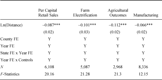
Table 3, shows the first-stage results used in the estimation of equation 4 for each sample. Each regression includes the full set of fixed effects and pretreatment covariates interacted with year indicators. The standard errors are clustered at the county level to allow for arbitrary correlation within counties over time. We should have only one first-stage estimate but as noted above, the sample varies due to missing values for dependent variables. Across the samples, the first-stage F-statistic ranges from 16 to 21, which suggest that there is not weak instrument bias if one is willing to accept weak instrument bias of no more than 10 percent in Stock-Yogo tests. Second, across the samples again, distance from a TVA dam reduces the likelihood the TVA delivers electricity to that county, Column 1 presents the results for the per capita retail sales sample with the inclusion of all instruments. In the per capita retail sales sample, a one-standard-deviation increase in distance from a TVA dam (about 260km), makes a county 22.6 percent less likely to enter into a power contract with the TVA.
Comparing the OLS and IV Results
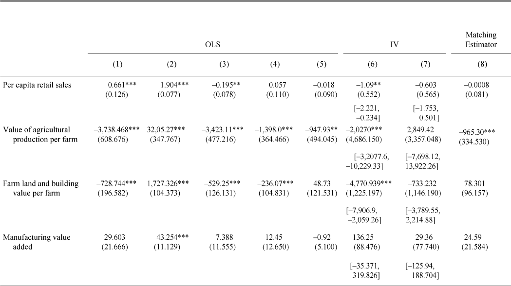
The main results are presented in Table 4. Standard errors, clustered at the county level, are reported in parenthesis. Below the IV specifications, in square brackets, I present robust confidence intervals based on a conditional likelihood ratio test developed by Marcelo Moriera (Reference Moriera2003).
Each row of the table corresponds to a different outcome. Columns 1 through 5 present the OLS results, adding additional fixed effects and covariates to each specification, while columns 6 and 7 present the IV results with the inclusion of county-fixed effects, year-fixed effects, and state-by-year fixed effects.
FIRST-STAGE REGRESSION RESULTS: THE EFFECT OF DISTANCE ON TVA POWER CONTRACTS

* p < .1.
** p < .05.
*** p < .01.
Note:
The dependent variable is a binary variable equal to 1 if the county has a TVA contract by in the given year and is zero otherwise. The Stock-Yogo Value for 10 percent bias is 16.38 and each regression includes the full set of fixed effects and controls X, which include the county electrification rate, the percent of the population living in urban areas, the change in urbanization from 1920–1930, population density, the number of families in each county, the age distribution, percent of population foreign born, percent of the population black, the percent of the population married and divorced, the number of farms, the average size of farms, the per capita crop value, the share of tenant farmers, percent of population that is illiterate, unemployment rate, percent of population owning radios, and the share of the population that voted in 1928 interacted with year fixed effects to allow them to have a different effect in each time period.
In row 1, I present the results for per capita retail sales, the broadest measure of economic activity. In column 1, the naive OLS results show a strong positive relationship between retail sales per capita and TVA electric contracts. When county-fixed effects are included, the magnitude of the relationship increases, likely capturing the growth of per capita retail sales coming out of the Depression, however, when year effects are included, eliminating nationwide increases, the sign flips and the correlation becomes strongly negative. Upon the inclusion of state-by-year fixed effects, the within-county correlation over time becomes positive, yet statistically insignificant. Finally, when adding pretreatment covariates, the correlation becomes negative.
SECOND-STAGE RESULTS: THE EFFECT OF THE TVASECOND-STAGE REGRESSION RESULTS


* p < .1.
** p < .05.
*** p < .01.
Note:
Each entry is from a separate regression and reports the coefficient of the TVA treatment variable. Standard errors are clustered at the county level to allow arbitrary correlation within the county over time. In square brackets, I present confidence intervals based on Moriera (Reference Moriera2003) conditional likelihood ratio test. Descriptions of each outcome variable are provided in the text.
In the IV specifications, Columns 6 and 7, the estimates are negative, and in the most robust specification, negative and statistically insignificant. The same trend can be found for agricultural production per farm (row 2), the value of land and equipment (row 3), manufacturing value added (row 4), and manufacturing employment (row 5). In all cases, the estimated coefficients increase in magnitude when I include county- fixed effects, decrease when I add year effects, and increase with state-by-year effects. There is some evidence that agricultural productivity declined, as the value of farm products and the value of farm land were negative. In the most robust OLS specification, that accounts for preexisting differences, agricultural production decreased. There is also some weak evidence that the TVA led to faster rural electrification, however, like the other outcomes, the result is not robust to the inclusion of pretreatment covariates. For each outcome, there is not strong evidence that the TVA power contracts improved conditions.
The results presented thus far are somewhat different from those found in KM who note that the TVA led to decreases in agricultural employment, increases in manufacturing employment, and increases in income. To ensure that the identification strategy is not driving the difference in the results, I implement a matching estimator similar to the one they suggest and reestimate my primary results, which are presented in column 8 of Table 4.
For the matching estimator, I first estimate the probability that a county will be part of the TVA by the end of my sample using a logit regression and all of the pretreatment covariates. I then obtain the propensity score. I then use the propensity score the regression weight for each observation. In this regression, I include county-fixed effects, year-fixed effects, and state-by-year fixed effects. The results in column 8 of Table 4 are qualitatively similar to the OLS results presented in column 5. I do not find statistically significant relationships between the TVA and economic activity, with the exception of a decrease in agricultural productivity. This leads me to believe that KM's broader treatment definition could be capturing the presence of spillovers associated with dam construction, as described by Severini (Reference Severini2012).
Given the lack of a strong statistical link between the TVA and economic growth in the Tennessee Valley, the historic legacy of the TVA must be explored in more depth. The TVA was supposed to be FDR's crown jewel in his efforts to weaken private power interests, provide power to the ordinary man, and stimulate the lagging Southern economy. Yet the results are, for the most part, inconclusive, making it difficult to rule out whether or not the TVA had large positive or negative effects. In the section that follows, I look for evidence that the TVA performed different functions from the preexisting private utilities and other New Deal agencies, such as the REA.
THE TVA POWER PROGRAM: A CLOSER EXAMINATION
The lack of a strong statistical relationship between the TVA and economic growth raises the question:could it be that the TVA was ineffective?The archival records of the TVA provide some clues of why the TVA had little measurable effect on economic performance.
The classic story of the TVA describes it as a key promoter of growth and rural electrification in the South, constructing dams to power new industry in the valley. However, this view is suspect because the private sector was quite active in the Tennessee watershed prior to 1933 and purchase agreements shaped most of the TVA's customer base such that it mirrored the markets served by private utilities.
Private firms had launched aggressive electrification plans in the South prior to the World War I. Alabama Power owned the Wilson Dam construction site and had options on the Wheeler Dam location (Martin Reference Martin1953).Footnote 15 Similarly, TEPCO owned the Norris Dam location and filed several applications with the FPC to acquire the rights to construct dams at other locations on the Tennessee River. Private utilities also began investing in rural electrification; Alabama Power created a special rural electrification initiative in the 1920s connecting the first farms to the grid in Alabama. Rural transmission and distributionconstruction continued to grow into the 1930s. Alabama Power constructed over 286 miles in 1935, and over 1,300 miles in 1936 (TVA 1937). By comparison, the TVA constructed 93 miles of rural line in 1934 and 200 miles in 1935. In fact, given the difference in land areas, both the TVA and Alabama Power extended rural electric service at about the same pace per square mile of territory (TVA 1934, 1935).
Limited rural service was available during the 1920s from firms such as Alabama Power and TEPCO, however their rates may have been prohibitively expensive. This was certainly true early on, but over time urban systems extended lines into rural area, which gave them access to residential service. Residential rates steadily fell throughout the 1920s and 1930s. Table 1 provides a sketch of the rural rates charged by Alabama Power to customers (famers and others) served by rural lines in 1929 (Edison Electric Institute 1929, p. 7). Under these rates, 100 kilowatt hours (KwH) a month would have cost $3.28 for electric usage plus an additional fee of $1.44–$3.28 to cover the cost of rural distribution line construction (1940 dollars). The total bill for these consumers ranged from 9–12.5 percent of monthly family income depending on the density of their electric line. By 1940 the cost had fallen to $3.50 for the same service, or about 6.6 percent of monthly income, with line charges eliminated. This decrease was consistent with the nationwide fall over the same period. Beginning in 1924, the average cost of 100 kWh was $6.67. By 1932 before the creation of the TVA, rates had fallen to about $5.53 for the same usage.Footnote 16 The price reductions came from reductions in management cost due to consolidations, changes in the generating sources, and improvements in generation and transmission technology.Footnote 17 The adoption of large coal-fired plants led to electric rates that were among the lowest in the nation.Footnote 18
In 1933 CS dropped its residential rates sharply. To many observers, the cut appeared to be a preemptive response to the inevitable creation of the TVA. However, the rate cut was not a response to pending TVA legislation since it had been scheduled by the company as part of the merger that created it in 1930. Furthermore, the rate cut was implemented throughout the entire CS system. CS noted that their southern subsidiaries were the industry leader throughout the 1920s, having pioneered low rate high volume pricing prior to the establishment of the TVA.Footnote 19 When transfers from CS to TVA occurred in 1934, 1936, and 1939, reduced rate schedules implemented by CS had already been in place for several years, both in the locations that went to TVA and those that stayed with CS.
While TVA advertised its promotional rate structure, the transfer of private assets to the TVA and municipal systems hid a portion of the price charged to the end consumer. To become a municipal system, a town had to first vote to become a municipal system, and if the ballot initiative passed, had to either construct its own lines or purchase existing distribution lines from the private utilities. Given the waste associated with duplication, most towns sought to purchase assets from the private utilities, although some strategically applied for PWA loans to threaten duplication. It was often difficult for municipalities to raise funds to purchase the distribution systems at the height of the Depression, as many investors did not want to purchase municipal bonds. In these cases, the TVA stepped in and purchased the generation, transmission, and distribution assets from the private utilities, and then sold off local distribution systems to municipalities to be paid back in installments. These payments were made through a series of separate charges listed on residential power bills.
The 1934 TVA annual report outlines the amortization fees and other surcharges when applicable (TVA Annual Report 1934, pp. 35–36). Amortization fees of one cent per kilowatt hour for the first 100 kWh with a minimum 25 cent fee were due each month in addition to the usage charge until the debt was repaid (TVA Annual Report 1937, p. 278). By 1956 only 37.5 percent of TVA distributors had paid off investments made on their behalf by the TVA (TVA 1956, pp. 8–9). This meant that for the bulk of TVA's service territory, the average monthly bill paid by customers was higher than promotional rate schedule advertised by the TVA.
Likewise, if the TVA aided the establishment of a cooperative utility, by selling acquired distribution resources or constructing rural lines, the cooperative had to pay the amortization fees. Cooperative utility members were also subject to a membership fee. As an example, I highlight the first cooperative to contract with the TVA, the Alcorn County Association, near Corinth, MS. To create the Alcorn cooperative, TVA loaned the Alcorn cooperative $154,000 to buy the Corinth, MS coal-fired plant, operated by the Mississippi Power Company, and the municipal distribution system (See http://www.ace-power.com/about/history/). Customers had to pay the amortization fees, outlined above and the cooperative membership fee (either a discounted lump sum of $80 or by incremental charges included in the monthly billof 1 cent per kWh for the first 100 kWh) (TVA Annual Report 1935, p. 27). This became the model for cooperatives extending service prior to the REA.Footnote 20 Rural cooperatives were important to the development of electricity markets in the South, yet rural customers only comprised 18.5 percent of TVA's customer base (TVA 1940).Footnote 21 Similarly, rural cooperatives only account for up to 25 percent of the customer base in Alabama, Mississippi, and Georgia, and North Carolina, thus the composition of CS's and the TVA's systems was similar.Footnote 22
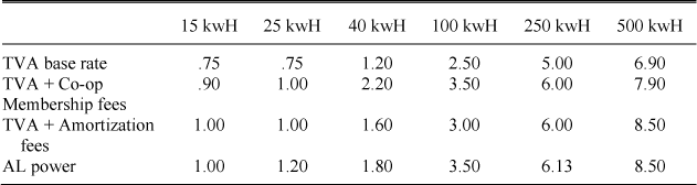
TYPICAL NET MONTHLY BILL TVA VS. ALABAMA POWER 1940

Sources:
U.S. Federal Power Commission 1940; TVA Annual Report 1937 pp. 277–89.
Provided that many of the TVA's distributers were required to pay amortization fees, cooperative membership fees, or both, the real rates paid by the TVA's consumers were actually much higher than those presented in Table 1. Table 5, reports the typical monthly bill in 1940 using the promotional rate schedule (row 1), includes cooperative membership fees (row 2), amortization fees (row 3), and compares them to the rates of Alabama Power (row 4) (U.S. Federal Power Commission 1940). When cooperative membership fees are added, the TVA rate is higher than the private utility rate for some ranges of consumption. When only amortization fees are included in the rate structure, the TVA rate is slightly lower than comparable private utility service. For the average level of consumption in 1940, 100KwH, TVA's rates were only 50 cents lower per month or about 1 percent of monthly income. For cooperative customers, at best, the rates were equal to those of Alabama Power, and potentially higher as some cooperative customers faced both amortization and membership fees (U.S. Federal Power Commission 1940).Footnote 23 Given the similarities of the customer base and the relatively small the price differentials, it seems unlikely that TVA electric contracts would have led spectacular increases in growth. While the price drop by the TVA was relatively small, the TVA could have expanded service to new customers, which would yield productivity gains.
The REA
The REA commands special attention in reference to the TVA. The REA was established in 1935 as a part of the Public Works Administration, and then created as its own agency in 1936. The REA provided loans to rural communities to construct electric distribution networks, wire homes, construct electric generation plants, and aid in the establishment of rural cooperative utilities. The REA initially had over $410 million ($6.5 billion in 2010 dollars) in federal appropriations at its disposal and by 1939 it established a network of over 350 electric cooperatives nationwide, providing an average of $350,000 per project (REA Annual Report 1939). In the Tennessee Valley, the TVA also provided some funding for the construction of distribution lines; however, they primarily focused on constructing dams and transmission lines. In 1935 the TVA's entire rural electrification budget was $84,000, less than 25 percent of a single REA project loan (TVA Annual Report 1935, p. 54).
In the Tennessee Valley, rural cooperatives served a relatively small population, yet played a crucial role in connecting new rural customers to the grid. Many of these cooperatives were established by the REA. In 1943 the REA provided financial statistics of its loan recipients, by then, forty cooperatives had signed wholesale power contracts with the TVA and 36 received loans from the REA for the construction of local distribution lines. Because the REA was so prominent in the area, it makes it difficult to disentangle the effects of the REA from the effects of the TVA. Fishback and Kitchens (Reference Fishback and Kitchens2013) find that the REA led to large increases in agricultural productivity in areas that received electricity, both in TVA counties and elsewhere, indicating that the REA may be the driver of growth, not the TVA. Given the limited funding devoted to rural electrification by the TVA, it is much more plausible that the REA was responsible for growth in rural connectionsand subsequent growth in the agricultural sector. Furthermore, the REA provided loans on an equal basis both in and outside of the TVA service area, which may explain the large aggregate increase in farm electrification rates from 1930–1950.
CLOSING REMARKS
Throughout the second half of the twentiethcentury, the TVA model has been viewed as a way to jumpstart the economy through the utilization of abundant water resources. The TVA injected over $20 billion into the Tennessee Valley from 1933 to 1960. Federal appropriations were used to construct dams, build transmission lines, and purchase existing capital from private firms. The TVA advertised low electric rates as a way to promote growth. New Dealers applauded the TVA for stimulating the economy in the Tennessee Valley, claiming that the TVA closed the income gap between the valley and the rest of the country.
However, upon careful examination of archival records, it can be seen that the TVA was primarily a wholesaler of electricity that was not active in local distribution. Furthermore, the TVA's low rates were not actually low relative to private firms in the region. After including amortization fees and cooperative membership fees, the average monthly bill of TVA consumers and private consumers were similar, and in some instances, TVA rates were higher. This discovery calls into question the ability of the TVA to act as an engine of growth, able to provide cheap energy inputs to farms and manufacturing. Additionally, other federal programs, such as the REA, played a major role in the construction of distribution infrastructure, that ultimately connected new customers to the grid.
To empirically explore the relationship between the TVA and economic outcomes, I constructed a panel of county level outcomes that measure broad based economic growth. Difference-in-Difference estimates, controlling for selection into TVA power contracts, show that the TVA did not have statistically significant impacts on per capita retail sales, rural electrification rates, agricultural production, agricultural land values, manufacturing value added, or manufacturing employment. While the empirical results are noisy, when combined with the archival records and the reconstructed rates, they suggests that the TVA's is not the engine of growth that it was previously believed to be.