1 Introduction
Environmental regulations impose severe restrictions on the emission of oxides of nitrogen from gas turbine engines. Operating the combustors at fuel lean conditions results in lower temperatures in the combustion zones, which subsequently reduces the emissions. However, at these conditions, combustors are susceptible to thermoacoustic instability (Lieuwen Reference Lieuwen2012). The occurrence of thermoacoustic instability is highly detrimental to the components and the performance of the combustor (Sujith, Juniper & Schmid Reference Sujith, Juniper and Schmid2016). Thermoacoustic instability arises from the coupling between the unsteady heat release rate of the flame and the acoustic field of the combustion chamber (McManus, Poinsot & Candel Reference McManus, Poinsot and Candel1993). Although active and passive control techniques exist to mitigate thermoacoustic instability (Schadow & Gutmark Reference Schadow and Gutmark1992; McManus et al. Reference McManus, Poinsot and Candel1993; Dowling & Morgans Reference Dowling and Morgans2005; Noiray et al. Reference Noiray, Durox, Schuller and Candel2009), it is still observed over a wide range of operating conditions and a better understanding of the complexities of the combustor is required to tackle this issue.
Traditionally, the transition from combustion noise to thermoacoustic instability has been regarded as a transition from a stable state to an unstable state, where the stable state is represented by a fixed point and the unstable state corresponds to limit cycle oscillations (Lieuwen Reference Lieuwen2002). However, Nair et al. (Reference Nair, Thampi, Karuppusamy, Gopalan and Sujith2013) suggested an alternative point of view that the stable state in a turbulent combustor need not be considered as a fixed point, but rather characterized by chaotic acoustic pressure fluctuations. Tony et al. (Reference Tony, Gopalakrishnan, Sreelekha and Sujith2015), by employing surrogate analysis, showed that the acoustic pressure fluctuations during the stable state exhibit characteristics of high-dimensional chaos contaminated with white and coloured noise. Furthermore, in turbulent combustors, Nair, Thampi & Sujith (Reference Nair, Thampi and Sujith2014) showed that the transition from combustion noise to thermoacoustic instability occurs via intermittency. During intermittency, bursts of periodic dynamics alternating between epochs of aperiodic dynamics were observed in the signals of acoustic pressure fluctuations. Findings from this study suggest that en route to thermoacoustic instability, there is a gradual emergence of periodic dynamics amidst aperiodic dynamics. Along with the gradual emergence of ordered dynamics (periodic oscillations) in time, an emergence of order (or coherent dynamics) has also been detected in the spatial dynamics.
For instance, large coherent structures or vortices emerge in the turbulent flow field and influence the flame dynamics during the state of thermoacoustic instability (Poinsot et al. Reference Poinsot, Trouve, Veynante, Candel and Esposito1987; Schadow et al. Reference Schadow, Gutmark, Parr, Parr, Wilson and Crump1989). Unni & Sujith (Reference Unni and Sujith2017) showed that the formation of large scale vortices and their interaction with the flame front causes a periodic heat release rate during the occurrence of intermittency. The evolution of large scale vortices (or large scale coherent structures) downstream of the backward-facing step appears to follow that of convectively unstable flows (Lieuwen Reference Lieuwen2012; Manoharan & Hemchandra Reference Manoharan and Hemchandra2015) where the disturbances are amplified as the flow propagates. A recent study by Kirthy et al. (Reference Kirthy, Hemchandra, Hong, Shanbhogue and Ghoniem2016) on a backward-facing step combustor reported that spatial amplification of velocity disturbances in a globally stable but locally convectively unstable flow could result in thermoacoustic instability. Further, Mondal, Unni & Sujith (Reference Mondal, Unni and Sujith2017) recognized that during the occurrence of thermoacoustic instability, the instantaneous relative phases between the acoustic pressure oscillations and the local heat release rate fluctuations exhibit spatial synchrony. During the occurrence of intermittency, regions of synchrony exist amidst regions of asynchrony, resembling a chimera state.
Thermoacoustic instabilities are driven by the interactions between the subsystems, namely the flow field, the acoustic field and the flame. A vortex is formed periodically in the flow field which entrains the reactants and hot products into itself. This mixture subsequently reacts. The consequent unsteady heat release rate excites the acoustic modes periodically, which perturbs the flow to cause the formation of the next vortex. However, in reality this interaction could be more intricate and intertwined during the transition to thermoacoustic instability. The interaction between the flame, the acoustic field and the hydrodynamic field is not unidirectional but mutual. Further, the interactions take place between all the three subsystems at every instant, throughout the reactive flow field.
Essentially, the interactions between the subsystems give rise to complexities in the spatial and temporal dynamics. Previous studies have shown that spatially extended coupled systems composed of multiple components and many degrees of freedom exhibit complex behaviour. For example, Liu et al. (Reference Liu, Dietz, Carpenter, Alberti, Folke, Moran, Pell, Deadman, Kratz and Lubchenco2007) observed complex patterns emerging due to coupling between human and natural systems in the study of the relationship between ecology and social sciences. Similarly, in a turbulent combustor, the hydrodynamic field, the flame and the acoustic field are coupled to each other. The rich spatial and temporal dynamics observed in the turbulent reacting flow is essentially the result of the interactions between these subsystems. In our paper, we investigate the spatio-temporal dynamics to extend the understanding of the coupling between the subsystems and the interactions within each individual subsystem, during the transition to thermoacoustic instability. To this end, we characterize the order emerging in the spatio-temporal dynamics en route to thermoacoustic instability as patterns emerging in the thermoacoustic system.
The flame in a turbulent combustor has a spatial structure or pattern which determines the resulting distribution of the heat release rate. Previous studies have shown that, due to spontaneous instabilities in premixed flames, smooth flames break into cellular flames which modifies the structure of the flame (Sivashinsky Reference Sivashinsky1983). Bayliss & Matkowsky (Reference Bayliss and Matkowsky1991) investigated the development of such spatial and temporal patterns in gaseous combustion through analytical and numerical studies.
The Cambridge dictionary (dictionary.cambridge.org) defines a pattern as any regularly repeated arrangement, especially a design made from repeated lines, shapes or colours on a surface. However, in the context of pattern formation literature, patterns can also be complex and irregular such as spatio-temporal chaos (Cross & Hohenberg Reference Cross and Hohenberg1994). In dynamical systems, patterns can appear both in time and in space. Pattern formation can either be the result of the occurrence of self-organization in the system or of external forcing. The Belouzov–Zhabotinsky and the Rayleigh Bénard systems are two canonical examples of systems that exhibit pattern formation (Busse Reference Busse1978; Croquette Reference Croquette1989a ,Reference Croquette b ). Various critical transitions which occur in biological systems, ecological systems etc., have been studied using the theory of pattern formation. Ball & Borley (Reference Ball and Borley1999) present an exhaustive study on fluid systems, biological systems, socio-economic systems, ecological systems etc., where spatio-temporal patterns have been observed. Further, Cross & Hohenberg (Reference Cross and Hohenberg1993) refer to various examples in hydrodynamics, nonlinear optics, biological systems etc., to illustrate complex patterns such as waves, spatio-temporal chaos, periodic and non-periodic patterns, scale-free patterns etc., observed in these systems.
Pattern formation in fluids has received a lot of attention in recent decades (Gollub & Langer Reference Gollub and Langer1999). Jakubith et al. (Reference Jakubith, Rotermund, Engel, Von Oertzen and Ertl1990) studied a reaction–diffusion system with catalytic oxidation of carbon monoxide in the presence of a platinum catalyst. This is a well-studied experimental system where many phenomena of non-equilibrium pattern formation have been observed. They observed that, with sufficiently high feedback intensities, chemical turbulence (having characteristics of spatio-temporal chaos) was replaced with another complex spatio-temporal pattern formed on the reactive surface. Previous studies have also depicted the emergence of patterns in fluid flow due to acoustic driving (Valverde Reference Valverde2015). In essence, patterns emerge in spatially extended, dissipative systems, when they are driven far from equilibrium (Staliunas & Sanchez-Morcillo Reference Staliunas and Sanchez-Morcillo2003). These patterns are often a result of instabilities in the system as a control parameter is varied beyond a critical value. Pattern formation theory is widely used to study critical transitions in ecological systems. In ecological systems, the driving forces of the instabilities which result in patterns, are positive feedbacks that operate at small spatial scales which give rise to spatial self-organization at large scales (Meron Reference Meron2016). In the context of a turbulent combustor, the local heat release rate which is due to reactions at the molecular scale drives the acoustic field of the combustor which has a much larger length scale, of the order of the length of the combustor, typically a few metres. Such similarities between the spatio-temporal dynamics observed in pattern forming systems and that observed in turbulent combustors advocate the use of pattern formation theory in understanding the transition in thermoacoustic systems.
Identifying, understanding and suppressing the spatial and temporal patterns in the flow field, the acoustic field and the flame structure are critical for preventing the transition from combustion noise to thermoacoustic instability. For example, a standing wave pattern in a rocket engine was suppressed by the insertion of baffles in the combustion chamber (Culick & Yang Reference Culick and Yang1995). Large amplitude pressure oscillations were suppressed by disrupting the formation of coherent vortices in the flow field (Paschereit & Gutmark Reference Paschereit and Gutmark2006). Samarasinghe et al. (Reference Samarasinghe, Culler, Quay, Santavicca and O’Connor2017) observed that the regions where the heat release rate were in phase with the pressure fluctuations, fluctuate out-of-phase with the pressure oscillations on the introduction of fuel staging, thereby causing suppression of thermoacoustic instability. Understanding the emergence of spatio-temporal patterns could possibly aid in the mitigation of thermoacoustic instability in turbulent combustors. Further, understanding the evolution of these spatio-temporal patterns could also pave the way for studies on early warning measures based on the emergence of these patterns.
Combustion noise exhibits irregular temporal (Nair & Sujith Reference Nair and Sujith2014; Tony et al.
Reference Tony, Gopalakrishnan, Sreelekha and Sujith2015) and spatio-temporal dynamics (Kheirkhah et al.
Reference Kheirkhah, Geraedts, Saini, Venkatesan and Steinberg2016; Mondal et al.
Reference Mondal, Unni and Sujith2017). In our study, during the occurrence of combustion noise, we observe disordered spatio-temporal dynamics. Incoherent production or absorption of acoustic power is observed during the epochs of aperiodic fluctuations. There is an intermittent emergence of ordered dynamics and a loss of chaos with the onset of intermittency. During the periodic oscillations, we observe the phenomenon of collective interaction of small scale vortices leading to the emergence of large scale vortices. Simultaneously, we also observe coherent regions of local acoustic power production (
 $p^{\prime }$
and
 $\dot{Q}^{\prime }$
in phase). Subsequently, chaotic dynamics is replaced by ordered or periodic spatio-temporal patterns during thermoacoustic instability.
In the present paper we examine the spatio-temporal dynamics and pattern formation in the subsystems during the transition from combustion noise to thermoacoustic instability. Section 2 gives a brief description of the experimental set-up and the data acquisition systems used in this study. Section 3 describes the results and observations from our experimental study. We describe and display the emerging spatio-temporal patterns during the onset of thermoacoustic instability. Further, we explain the manner in which pattern formation theory provides an alternative perspective of how the interactions within the reactive flow field which occur at smaller spatial and temporal scales lead to order at larger spatio-temporal scales. In addition, we also use indicators of pattern formation to detect the emergence of spatial and temporal patterns in the turbulent combustor. Finally, we conclude with the key findings from this study in § 4.
2 Experimental set-up
The combustor used for the present study is shown in figure 1(a). Figure 1(b) shows a technical drawing of the experimental set-up along with the dimensions of the combustion chamber and the location of the bluff body. It is a turbulent combustor with a backward-facing step and a bluff body to stabilize the flame. The bluff body is a circular disk of 47 mm diameter and 10 mm thickness and it is mounted on a central shaft which is 16 mm in diameter. The bluff body is located 45 mm from the backward-facing step. The hollow central shaft delivers the fuel into the burner through four radial injection holes of 1.7 mm located 110 mm upstream of the dump plane. Compressed air is injected into the plenum chamber and it is partially premixed with the fuel in the burner before the mixture enters the combustion chamber. Liquefied petroleum gas (LPG) (60 % butane and 40 % propane) is used as the fuel for this study. The combustible mixture is ignited by a spark provided by a spark plug connected to an ignition transformer (11 kV). The combustion chamber has a cross-section of
 $90\times 90~\text{mm}^{2}$
and it is 1100 mm long. A decoupler (
 $1000~\text{mm}\times 500~\text{mm}\times 500~\text{mm}$
) is connected to the end of the combustion chamber to reduce acoustic energy losses through acoustic radiation.
(a) Schematic of the turbulent combustor. A bluff body is used for flame stabilization. The design of this combustor was adapted from Komarek & Polifke (Reference Komarek and Polifke2010). A pressure transducer is used to measure the unsteady pressure fluctuations in the combustor duct while a PMT records the global heat release rate fluctuations. Particle image velocimetry experiments are performed using an Nd:YLF laser which illuminates the seeding particles. A high-speed camera captures the Mie scattering light from the seeding particles. Another high-speed CMOS camera captures
 $\text{OH}^{\ast }$
chemiluminescence from the flame. (b) Technical drawing of the experimental set-up used for this study. The bluff body is located 45 mm from the dump plane. Fuel is injected 110 mm upstream of the dump plane and subsequently, mixing with air takes place.

The mass flow rates of fuel and air are controlled and measured using mass flow controllers (Alicat Scientific, MCR Series) which have an uncertainty of
 $\pm 0.8\,\%$
of the reading
 $+0.20\,\%$
of the full scale. The subsequent uncertainty in the Reynolds number
 $Re$
is approximately
 $\pm 6\,\%$
for all the flow rates reported here. In this study, we discuss the results obtained at various equivalence ratios of the reactant mixture. The equivalence ratio is estimated as
 $\unicode[STIX]{x1D719}=({\dot{m}}_{f}/{\dot{m}}_{a})_{actual}/({\dot{m}}_{f}/{\dot{m}}_{a})_{stoichiometric}$
(where
 ${\dot{m}}_{f}$
is mass flow rate of fuel and
 ${\dot{m}}_{a}$
is mass flow rate of air). The uncertainty in the estimated equivalence ratio is
 $\pm 0.02$
. A piezoelectric transducer (PCB103B02 – uncertainty
 $\pm 0.15$
Pa) is mounted on the combustor wall using an external waveguide (35 mm height), located 17 mm from the dump plane to measure the unsteady pressure fluctuations. We observe that the mounting arrangement of the transducer results in less than 5 degrees phase shift for the acoustic oscillations at the dominant frequency. This is not significant enough to affect the analyses reported in this study. A photomultiplier tube (PMT) module mounted with an
 $\text{OH}^{\ast }$
filter (narrow bandwidth filter centred at 308 nm and 12 nm FWHM) captures the global unsteady heat release rate (
 $\dot{q}^{\prime }$
). The PMT module has a field of view of 70 degrees which encompasses the entire quartz duct. The signals from the piezoelectric transducer and the PMT module are acquired using an A-D card (NI-6143, 16 bit) at a sampling frequency of 10 kHz, for three seconds.
High-speed
 $\text{OH}^{\ast }$
chemiluminescence images, used to obtain the local unsteady heat release rate (
 $\dot{Q}^{\prime }(x,y)$
) of the flame, are acquired using a high-speed CMOS camera (Phantom – v 12.1) operating at a frame rate of 2 kHz and
 $800\times 527$
pixels resolution. The exposure time is fixed as 499
 $\unicode[STIX]{x03BC}\text{s}$
. The camera is equipped with a ZIESS 50 mm camera lens at
 $f/2$
aperture. In this manner, a
 $67~\text{mm}\times 44~\text{mm}$
region of the optically accessible section of the combustor duct is imaged onto
 $800\times 527$
pixels of the camera sensor. The area of the test section spans a region 23 mm downstream of the dump plane. The flame images are captured through a narrow bandwidth filter centred at 308 nm (12 nm FWHM) corresponding to
 $\text{OH}^{\ast }$
chemiluminescence. A total of 5000 images are captured at each equivalence ratio.
High-speed particle image velocimetry (PIV) is performed to acquire velocity field measurements.
 $\text{TiO}_{2}$
particles (Kronos make – product – 1071) of approximate size 1
 $\unicode[STIX]{x03BC}\text{m}$
are seeded into the reactive flow field (80 % of the particles are between the size of 0.2 and 2
 $\unicode[STIX]{x03BC}\text{m}$
. The median size of the particles is 0.61
 $\unicode[STIX]{x03BC}\text{m}$
). We use this size for seeding the flow so that the particles faithfully track the fluid flow. The Stokes number (
 $St=t_{0}/(l_{0}/t_{0})$
,
 $t_{0}=(\unicode[STIX]{x1D70C}_{p}{d_{p}}^{2}/18\unicode[STIX]{x1D707}_{g})$
where
 $t_{0}$
is the characteristic response time of the particle,
 $u_{0}$
is the gas velocity,
 $l_{0}$
is the characteristic dimension of the obstacle,
 $\unicode[STIX]{x1D70C}_{p}$
is the particle density,
 $d_{p}$
is the particle diameter and
 $\unicode[STIX]{x1D707}_{g}$
is the fluid viscosity) for the
 $\text{TiO}_{2}$
particles used in our study is calculated to be
 $7\times 10^{-4}$
. The particle phase is in a suspension form. Hence, two-way coupling effects where the particles could affect the flow dynamics are possible (Sirignano Reference Sirignano2010). However, the overall dynamics does not appear to be affected and we observe the distinct states of combustion noise, intermittency and thermoacoustic instability. Due to the small size of the particles, the test section windows become clouded quickly. To avoid this, the experiments at different equivalence ratios are performed in a discontinuous manner.
A single cavity-double pulsed Nd:YLF laser (Photonics) of operating wavelength 527 nm operating at a repetition rate of 2 kHz and a pulse duration of 200 ns produces twin pulses to illuminate the seeding particles. The laser beam is directed towards the combustion chamber using a set of right angle prisms and convex lenses (500 mm and 50 mm). The laser beam is then expanded into a laser sheet of 2 mm thickness using 600 mm spherical and
 $-16$
mm cylindrical lenses. This laser sheet is transmitted through a horizontal slit (5 mm width and 400 mm length) made of quartz on the top plate of the duct into the combustion chamber. The time delay between the two pulses is carefully chosen between 15 and 25
 $\unicode[STIX]{x03BC}\text{s}$
for various equivalence ratios such that the maximum pixel displacement of the particles between the two laser pulses is approximately between 4 and 7 pixels. We ensure that the maximum particle displacement does not exceed
 $1/4$
th of the size of the interrogation window. Such parameters are chosen to avoid loss of correlation of in-plane particles during the PIV evaluation. The light scattered by the seeding particles (Mie scattering) is captured by a high-speed CMOS camera (Photron FASTCAM SA4) synchronized with the laser onto a sequence of frames. The camera is equipped with a ZEISS 100 mm lens with the aperture at
 $f/5.6$
. The Photron camera can be operated at a maximum of
 $1024\times 1024$
pixels resolution. The image pairs are captured at 1 kHz. In our experiments, a measurement region of
 $31~\text{mm}\times 63~\text{mm}$
is imaged on to
 $500\times 1024$
pixels of the sensor. The region where PIV is performed is situated at the centrespan of the bluff body. A short bandpass optical filter centred at 527 nm (12 nm FWHM) is mounted in front of the lens to capture the Mie scattering light. The scattered light from the particles is distributed over 1.5 to 2.5 pixels. The measurement uncertainty in the pixel displacement associated with this range of particle image diameter due to peak locking is less than 0.03 pixels (Raffel, Willert & Kompenhans Reference Raffel, Willert and Kompenhans2007). The average particle image density is approximately 4 particles per interrogation window in the recirculation (low velocity) regions and 9 particles per interrogation window for the bulk flow (high velocity) regions. Higher density of seeding particles was not possible due to clouding of test section windows. The peak ratio for the velocity data illustrated in this study is in the range of 7 to 30 for the large velocity regions. However, for the low velocity regions, the lower limit of the peak ratio reduces to a low value of 2.
The Mie scattering images are processed using PIVview software (PIVview 2014). The velocity field is evaluated from the Mie scattering image pairs using a cross-correlation algorithm with a grid refining multipass approach and the least square Gaussian fit peak search scheme (Raffel et al.
Reference Raffel, Willert and Kompenhans2007). The grid refining multipass approach is started with
 $192\times 192$
pixels grid size. The final grid size is
 $32\times 32$
pixels for low flow rates (
 $\unicode[STIX]{x1D719}=0.96$
and
 $\unicode[STIX]{x1D719}=0.83$
). Further, 50 % overlap is chosen between the interrogation windows. However, for high flow rates (
 $\unicode[STIX]{x1D719}=0.63$
), the initial grid size is chosen as
 $192\times 192$
pixels followed by 4 passes with a final grid size of
 $48\times 48$
pixels to reduce in-plane loss of correlation. At these high flow rates, 65 % overlap is chosen between the interrogation windows. Ideally, the pixel displacement should be
 $1/4$
th of the size of the interrogation windows for the PIV evaluation. However, we are restricted in reducing the size of the interrogation windows (to obtain pixel displacement of 1/4th of the size of the interrogation window) due to medium density of particles in the field of view which could result in more outliers. We are restricted in increasing the seeding density of the particles as it causes faster clouding of the quartz ducts. The grid size and the overlap are chosen in such a way that the resolution of the velocity field is approximately the same for all the flow rates. This results in a vector spacing of approximately 1 mm for all the flow rates.
A number of post-processing algorithms are used to detect and replace a small number of spurious vectors. Firstly, the maximum displacement test is used with appropriate thresholds for different flow rates to detect spurious vectors (Raffel et al.
Reference Raffel, Willert and Kompenhans2007). This is based on the expected bulk flow velocities in the test section. Secondly, a vector difference filter which calculates the magnitude of the vector difference of a particular vector in question to each of its 8 neighbours is also used to detect spurious vectors (Raffel et al.
Reference Raffel, Willert and Kompenhans2007). A threshold of 2 pixels is chosen for the vector difference filter. In total, less than 1 % of the total velocity vectors are detected as spurious vectors and replaced with a bilinear interpolation method. Much of the uncertainty from this PIV evaluation arises out of the choice of the short pixel displacement. For the chosen PIV evaluation methods, estimation accuracies of the order of
 $1/10$
th to
 $1/20$
th of a pixel are realistic for
 $32\times 32$
pixel samples from 8-bit digital images. The velocity uncertainty in our study is approximately between 1.25 % and 2.5 % based on subpixel resolution between 0.05 and 0.1 pixels for
 $32\times 32$
interrogation windows (Raffel et al.
Reference Raffel, Willert and Kompenhans2007) for low flow rates where the size of interrogation windows is
 $32\times 32$
pixels. Further, particle displacement as small as 0.2 pixels in the low velocity recirculation and wake regions results in velocity uncertainties of 50 % in these regions.
We use a vortex detection scheme to detect the vortices in the flow field obtained from the PIV measurements (Schram, Rambaud & Riethmuller Reference Schram, Rambaud and Riethmuller2004; Varun, Balasubramanian & Sujith Reference Varun, Balasubramanian and Sujith2008). It uses the discriminant
 $d_{2}$
of the non-real eigenvalues of the velocity gradient matrix. For an incompressible flow,
 $d_{2}$
is calculated as
 $d_{2}=-4(u_{x}v_{y}-u_{y}v_{x})$
. The calculated eigenvalues are complex if
 $d_{2}$
is negative and these complex eigenvalues will result in a local spiral pattern of the streamline (Vollmers Reference Vollmers2001). Hence, one can consider the region with negative
 $d_{2}$
to be the vortex core. Firstly, the
 $d_{2}$
field is calculated for the velocity measurements obtained from PIV. Next, the wavelet transform of the
 $d_{2}$
field is evaluated using the Mexican hat as the mother wavelet. Previous studies have used the Mexican hat wavelet as the mother wavelet for the detection of vortex cores and the corresponding sizes (Schram & Riethmuller Reference Schram and Riethmuller2001). The local maxima of the wavelet transform of the
 $d_{2}$
field corresponds to the centre of the vortices. The scales corresponding to the maximum value of the wavelet transform are then selected to calculate the size of the vortices. A global threshold of the transformed
 $d_{2}$
field is also used to filter out vortices of lower strength. For more information on the detailed procedure of the eduction of vortices, we refer to the work by Schram & Riethmuller (Reference Schram and Riethmuller2001) and Varun et al. (Reference Varun, Balasubramanian and Sujith2008).
The Mie scattering technique using oil droplets has been used in the recent years to qualitatively describe the flame front (Shanbhogue et al.
Reference Shanbhogue, Shin, Hemchandra, Plaks and Lieuwen2009; Zhang, Shanbhogue & Lieuwen Reference Zhang, Shanbhogue and Lieuwen2010; Kheirkhah & Gülder Reference Kheirkhah and Gülder2013; Shin & Lieuwen Reference Shin and Lieuwen2013). We perform separate Mie scattering experiments at selected equivalence ratios using olive oil droplets of approximate size 1
 $\unicode[STIX]{x03BC}\text{m}$
(Gurubaran Reference Gurubaran2005) to describe the collective interaction of small scale vortices to form large scale coherent structures. The incoming air is seeded with the olive oil droplets which are produced utilizing a Laskin nozzle. The oil droplets, while passing through the flame, evaporate and burn. When the oil droplets pass through a laser sheet, light is scattered. The boundary of the illuminated region represents the flame front since the oil droplets are present only in regions with cold unburned reactants. An Nd:YLF laser which is synchronized with a high-speed camera (Phantom v 12.1) in single pulse mode is used for the Mie scattering experiments. The images are acquired by the camera at 5000 f.p.s. for a duration of 1.5 s. The camera is outfitted with a ZEISS 100 mm lens with aperture at
 $f/2.8$
. In this manner, approximately
 $55~\text{mm}\times 34~\text{mm}$
of the combustor duct is imaged on to
 $1280\times 800$
pixels of the camera sensor. Even though other techniques such as Rayleigh scattering could provide a more accurate description, the Mie scattering technique in the experiments shown here is able to qualitatively capture the collective interaction of small scale vortices to form a large vortex.
3 Results
This experimental investigation is performed on a turbulent combustor with a bluff body stabilized flame to identify and characterize the spatio-temporal dynamics observed during different dynamical states en route to thermoacoustic instability. During this transition, the anchoring point of the flame shifts and this behaviour was investigated by Unni & Sujith (Reference Unni and Sujith2017) on the same combustor. A self-excited axial mode is observed from the flame dynamics during the occurrence of thermoacoustic instability. The fuel flow rate is maintained constant (
 ${\dot{m}}_{f}=0.875\times 10^{-3}~\text{kg}~\text{s}^{-1}$
which corresponds to a thermal power of 43.6 kW) and the air flow rate is varied in discrete steps. Consequently, the equivalence ratio (
 $\unicode[STIX]{x1D719}$
) is varied from 0.98 (
 $Re=12\,500$
) to 0.63 (
 $Re=18\,000$
). Due to the partially premixed nature of the reactants, local extinction events occur at equivalence ratios less than 0.3 (Unni & Sujith Reference Unni and Sujith2015), which is away from the operating conditions of the current study. Hence, the spatio-temporal dynamics discussed in this paper is not affected by the blowout dynamics. Further, local quenching (Poinsot, Haworth & Bruneaux Reference Poinsot, Haworth and Bruneaux1993) effects near the walls are not dominant and so do not prevent the transition from the stable state to the unstable state.
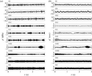
Time trace of the acoustic pressure fluctuations and the global heat release rate oscillations (obtained from PMT) acquired at various equivalence ratios
 $\unicode[STIX]{x1D719}=0.98$
(i),
 $\unicode[STIX]{x1D719}=0.94$
(ii),
 $\unicode[STIX]{x1D719}=0.9$
(iii),
 $\unicode[STIX]{x1D719}=0.87$
(iv),
 $\unicode[STIX]{x1D719}=0.83$
(v),
 $\unicode[STIX]{x1D719}=0.78$
(vi),
 $\unicode[STIX]{x1D719}=0.75$
(vii),
 $\unicode[STIX]{x1D719}=0.7$
(viii),
 $\unicode[STIX]{x1D719}=0.65$
(ix) and
 $\unicode[STIX]{x1D719}=0.63$
(x) for 3 s. It should be noted that the ordinates are different for better visual representation.
 $p^{\prime }$
has units of kPa while
 $\dot{q}^{\prime }$
has arbitrary units.

3.1 Evolution of spatio-temporal patterns
The acoustic pressure fluctuations (
 $p^{\prime }$
) and the global heat release rate fluctuations (
 $\dot{q}^{\prime }$
) obtained for various equivalence ratios are presented in figure 2. The
 $p^{\prime }$
and
 $\dot{q}^{\prime }$
signals are obtained by subtracting the mean from the instantaneous values. Both
 $p^{\prime }$
and
 $\dot{q}^{\prime }$
are aperiodic at
 $\unicode[STIX]{x1D719}=0.98$
corresponding to the regime of combustion noise. Pawar et al. (Reference Pawar, Seshadri, Unni and Sujith2017) showed that these signals are desynchronized temporally during this state. This aperiodic dynamics reflects the disordered and chaotic behaviour in the temporal dynamics of the turbulent combustor (Tony et al.
Reference Tony, Gopalakrishnan, Sreelekha and Sujith2015). Between
 $\unicode[STIX]{x1D719}=0.87$
and
 $\unicode[STIX]{x1D719}=0.7$
, we observe intermittent bursts of periodic oscillations amidst epochs of aperiodicity, previously described by Nair et al. (Reference Nair, Thampi and Sujith2014). The onset of intermittency corresponds to an onset of emerging order in the form of periodicity in the temporal dynamics. Pawar et al. (Reference Pawar, Seshadri, Unni and Sujith2017) showed that during this state, the
 $p^{\prime }$
and
 $\dot{q}^{\prime }$
signals are synchronized intermittently during the periodic bursts and desynchronized during the aperiodic epochs. At
 $\unicode[STIX]{x1D719}=0.63$
, thermoacoustic instability is observed. The aperiodic signals during combustion noise and intermittency are completely replaced by periodic temporal patterns during thermoacoustic instability, wherein
 $p^{\prime }$
and
 $\dot{q}^{\prime }$
are locked in. This illustrates a gradual emergence of periodicity in the temporal dynamics as
 $\unicode[STIX]{x1D719}$
is varied from 0.98 to 0.63.
For the spatial analyses which follow, to illustrate the phenomenon of pattern formation, we choose the equivalence ratios of 0.98, 0.83 and 0.63 which correspond to the states of combustion noise, intermittency and thermoacoustic instability respectively. Similar behaviour in the spatial dynamics is observed for the other equivalence ratios corresponding to each state.
3.1.1 Combustion noise
Instantaneous fields of local acoustic power production
 $p^{\prime }\dot{Q}^{\prime }(x,y,t)$
, are illustrated in figure 3(a–d) at different instants of time for
 $\unicode[STIX]{x1D719}=0.98$
. The instantaneous field of local acoustic power production is obtained as the product of the instantaneous pressure fluctuations,
 $p^{\prime }(t)$
and the instantaneous local heat release rate fluctuations,
 $\dot{Q}^{\prime }(x,y,t)$
obtained from the high-speed camera. Lieuwen & Zinn (Reference Lieuwen and Zinn2000) showed that if the length scale of the reaction zone is much less than the acoustic length scale, the variation of pressure across the reaction zone is small. Nair (Reference Nair2014) had also confirmed this experimentally in the same combustor used for this study. Further, as described in § 2, the chemiluminescence images are acquired for a small section of the combustion chamber where we do not expect
 $p^{\prime }$
to vary. Thus,
 $p^{\prime }(t)$
used for the calculation of
 $p^{\prime }\dot{Q}^{\prime }(x,y,t)$
is acquired using a single piezoelectric transducer near the dump plane.
(a–d) Instantaneous fields of local acoustic power production (
 $p^{\prime }\dot{Q}^{\prime }(x,y,t)$
) during the occurrence of combustion noise at
 $\unicode[STIX]{x1D719}=0.98$
for different instants of time
 $t$
. (e) The corresponding
 $p^{\prime }$
and
 $\dot{q}^{\prime }$
(obtained from PMT). Note that the colour bars used to indicate the local acoustic power production are different for the different time instants. The instantaneous fields of local acoustic power production appear seemingly grainy. The inset displayed in (a) represents a zoomed in view.
 $\dot{Q}^{\prime }(x,y,t)$
is obtained by subtracting the temporal mean at each location from the instantaneous value at that pixel location.

During the occurrence of combustion noise, the spatial distribution of
 $p^{\prime }\dot{Q}^{\prime }(x,y,t)$
appears grainy without any evident or distinct pattern for different instants of time. In other words, the value of
 $p^{\prime }\dot{Q}^{\prime }$
at one location and at one instant of time has non-similar values in its neighbourhood, which makes the field of local acoustic power production appear grainy. We call these grainy structures disordered patterns or incoherent patterns in the spatial dynamics of the turbulent reacting field. Even though the acoustic pressure fluctuations are chaotic and we observe irregular spatial dynamics during the occurrence of combustion noise, we cannot conclusively state the dynamical nature of the spatial structures as spatial chaos. However, spatio-temporal chaos has been observed in turbulent fluid systems which at certain conditions exhibit coherent behaviour. For example, Manneville (Reference Manneville2010) suggested that spatial chaos can be characterized by coherence at the local scale and incoherence at the global scale. There appears to be coherence or similar values for immediate neighbours when zooming in (refer to inset of figure 3
a) to very small scales while the spatial dynamics appears irregular at the larger scales. This behaviour during the occurrence of combustion noise suggests that the spatio-temporal dynamics could be spatio-temporal chaos.
(a–d) Instantaneous velocity vector fields during the occurrence of combustion noise, overlaid on the vorticity field. The region marked as grey is representative of the region occupied by the bluff body and areas with high reflection. The contours of the vortices detected by the vortex detection algorithm are coloured purple. We do not observe any large scale vortices upstream of the buff body in the shear layer region during the occurrence of combustion noise. The shear layer upstream of the bluff body can be identified by higher vorticity strength.

The instantaneous fields of velocity vectors corresponding to the same conditions as in figure 3(a–d) are shown in figure 4(a–d) overlaid on the vorticity field. These fields represent an area approximately 23 mm downstream of the dump plane. We do not observe any large scale vortices in figure 4. It should be noted that the smallest vortex that can be captured is limited by the resolution of the PIV. Some small scale vortices are observed just above the bluff body. These structures could form as a result of boundary layer separation from the bluff body.
(a–d) Instantaneous field of local acoustic power production
 $p^{\prime }\dot{Q}^{\prime }(x,y,t)$
at different instants of time
 $t$
during a periodic epoch of intermittency. (e) Simultaneous
 $p^{\prime }(t)$
and
 $\dot{q}^{\prime }(t)$
(obtained from PMT) corresponding to (a–d) are marked. Here,
 $p^{\prime }\dot{Q}^{\prime }(x,y,t)$
comprises of regions of coherent dynamics. During the periodic epochs, the values of
 $p^{\prime }\dot{Q}^{\prime }(x,y,t)$
are one order of magnitude higher than those during combustion noise. At
 $\unicode[STIX]{x1D719}=0.83$
, the emergence of correlated regions illustrates the emergence of coherence in the spatial dynamics of the turbulent thermoacoustic system. (f–i) Instantaneous field of local acoustic power production during the aperiodic regime of the intermittency. (j) Simultaneous
 $p^{\prime }(t)$
and
 $\dot{q}^{\prime }(t)$
(obtained from PMT). In general, we observe grainy structures upstream and downstream of the bluff body with clustered regions of low magnitude negative
 $p^{\prime }\dot{Q}^{\prime }$
downstream of the bluff body.

3.1.2 Intermittency
Figure 5(a–d) shows the instantaneous fields of local acoustic power production
 $p^{\prime }\dot{Q}^{\prime }(x,y,t)$
during a periodic epoch of intermittency at
 $\unicode[STIX]{x1D719}=0.83$
. Regions of coherent behaviour with large magnitude begin to emerge in the field of
 $p^{\prime }\dot{Q}^{\prime }(x,y,t)$
(refer to figure 5
d). One can observe a region upstream of the bluff body with a cluster of similar values of
 $p^{\prime }\dot{Q}^{\prime }$
. This clustering phenomenon observed in the spatial dynamics hints at self-organization and the emergence of localized coherent spatial structures amidst incoherent regions (grainy regions) (Mondal et al.
Reference Mondal, Unni and Sujith2017). In other words, the local interactions at the small scale in the field of
 $p^{\prime }\dot{Q}^{\prime }$
, enabled by the favourable local flame speeds, result in coherence at the large scale. Similar behaviour of the emergence of localized patterns was observed in an experimental study on pattern formation in the transverse acoustic pressure field (Sánchez-Morcillo et al.
Reference Sánchez-Morcillo, Martínez-Mora, Pérez-Arjona, Espinosa and Alonso2010). They observed that the localized structure emerges due to the effect of spatial coupling. Figure 5(f–i) shows the fields of
 $p^{\prime }\dot{Q}^{\prime }(x,y,t)$
obtained during an aperiodic epoch of intermittency. For all the instants of time depicted here, there appears to be very low acoustic power production. Coherence is observed at a large scale in figure 5(f) downstream of the bluff body although its magnitude is very low. Incoherent regions or grainy structures are observed upstream and downstream of the bluff body. Here, there are clustered regions of negative
 $p^{\prime }\dot{Q}^{\prime }$
around the bluff body. Further, one should note that in general, these regions of negative
 $p^{\prime }\dot{Q}^{\prime }$
during the aperiodic epochs of intermittency have higher magnitude than that of the state of combustion noise.
(a–d) Instantaneous velocity vector fields which are overlaid on the vorticity field during a large amplitude periodic epoch of intermittency. A large scale coherent structure with high vorticity strength is detected upstream of the bluff body in (c). (e–h) Instantaneous velocity fields corresponding to the aperiodic epoch of intermittency. Here, we do not observe large scale coherent structures upstream of the bluff body. The vorticity strength during these aperiodic oscillations is slightly higher than the strength observed during combustion noise in the shear layer region. These images correspond to the same instants of time as those shown in figure 5.

The instantaneous velocity fields during the periodic epoch of intermittency corresponding to the figure 5(a–d) are shown in figure 6(a–d). In these images, one can observe the emergence of relatively large vortices upstream of the bluff body (refer to figure 6
c). Large scale coherent structures promote entrainment and stirring at the macro-scale (Eckart Reference Eckart1948). Upon impingement or breakdown of these large structures, the fine scale turbulence enhances the diffusivity and, subsequently, molecular scale mixing (Eckart Reference Eckart1948). In this manner, in the turbulent combustor, the large coherent structures promote entrainment, stirring and, subsequently, mixing between the fresh reactants and hot products upon impingement. This initiates the combustion of the entrained fresh reactants causing heat release rate to occur in unison and to be localized. We conjecture that, at intermittency, the observed coherence or ordered dynamics of
 $p^{\prime }\dot{Q}^{\prime }(x,y,t)$
is due to this coherent heat release rate at an appropriate phase of pressure fluctuations resulting in the periodic pattern of the acoustic pressure oscillations.
During the aperiodic epochs of intermittency, we do not observe any large scale vortex in figure 6(e–h) similar to that observed during the periodic epochs of intermittency. However, we observe small scale vortices downstream and upstream of the bluff body. These vortices either do not grow in size or they vanish in consecutive time instants. Acoustic perturbations or heat release rate fluctuations could disrupt the vortex growth and cause the suppression of the growth of these structures (Renard et al. Reference Renard, Thevenin, Rolon and Candel2000). Similarly, in our turbulent combustor, it is probable that the shear layer is perturbed by the acoustic fluctuations and the baroclinic vorticity generated by the flame, leading to the suppression of the growth of unstable modes in the shear layer (Renard et al. Reference Renard, Thevenin, Rolon and Candel2000).
(a–f) Instantaneous fields of local acoustic power production
 $p^{\prime }\dot{Q}^{\prime }(x,y,t)$
at different instants of time (
 $t$
) during the occurrence of thermoacoustic instability for one periodic cycle. (g) Simultaneous
 $p^{\prime }(t)$
and
 $\dot{q}^{\prime }(t)$
(obtained from PMT). Here, we observe that the fields of
 $p^{\prime }\dot{Q}^{\prime }(x,y,t)$
comprise of regions of coherent dynamics.

3.1.3 Thermoacoustic instability
Figure 7(a–f) shows the fields of
 $p^{\prime }\dot{Q}^{\prime }(x,y,t)$
for one periodic cycle during the occurrence of thermoacoustic instability at
 $\unicode[STIX]{x1D719}=0.63$
. We observe large regions of coherent dynamics similar to that observed during the periodic epochs of intermittency. These coherent regions are observed mainly on top of the bluff body and downstream of the bluff body. The magnitude of the positive
 $p^{\prime }\dot{Q}^{\prime }(x,y,t)$
in these coherent regions is higher compared to that observed during the occurrence of intermittency. Further, the magnitude of the positive acoustic power in these coherent regions is significantly higher than their negative counterparts found in other regions of the reactive flow field.
The instantaneous velocity fields with detected vortices overlaid on the vorticity field in figure 8 show the emergence of large scale coherent structures upstream of the bluff body. In addition, the vorticity fields obtained during thermoacoustic instability show higher strength. Large vortices are also observed downstream of the bluff body, which are likely due to vortex shedding from the bluff body. At these low equivalence ratios, where thermoacoustic instability is observed, the temperature differences between the unreacted mixture and the hot products become small. It is possible that the resulting lower strength of baroclinic vorticity does not hinder the growth of the stronger large scale vortices. The large structures in figure 8(d,e) are detected with data smoothing of the velocity field using a Gaussian weighted kernel, prior to the calculation of the
 $d_{2}$
field in addition to the post-processing steps described in § 2 before the vortex detection procedure. This is to ensure a better eduction of the large scale structure observed in the velocity vector field (Varun et al.
Reference Varun, Balasubramanian and Sujith2008). One should note that when comparing figure 7(e,f) with the corresponding vorticity field in figure 8(e,f), regions with highest values of the local acoustic power production exist at regions of high vorticity downstream of the bluff body. One should also note that this occurs after the formation of the large vortex observed in figure 8(d) upstream of the bluff body and its subsequent impingement. Here, the strong interaction between the flow patterns and the spatial structure of the flame results in self-sustained periodic acoustic pressure oscillations.
A previous study by Ho & Nosseir (Reference Ho and Nosseir1981) observed the phenomenon of ‘collective interaction’ of small scale coherent structures impinging on a flat plate. These studies established that this process, termed collective interaction, closes the feedback loop between the convected coherent structures and the propagating pressure waves generated by the impingement of the coherent structures resulting in self-sustained oscillations. Additionally, they observed that due to this collective interaction, there is an emergence of a single dominant frequency. The observed large scale vortices in figure 6(c) during the periodic epoch of intermittency and that in figure 8(d) during thermoacoustic instability are likely to be the result of this collective interaction of multiple small scale vortices. This collective interaction process in the turbulent combustor is illustrated in detail in the next section.
(a–f) Instantaneous velocity vector fields during thermoacoustic instability (
 $\unicode[STIX]{x1D719}=0.63$
) overlaid on the field of vorticity. We can observe the emergence of a large vortex upstream of the bluff body larger than the vortices observed during the periodic epochs of intermittency. These images correspond to the same conditions as figure 7.

3.1.4 Self-organization leading to emergence of coherent structures in the flow field
(a) Perturbation of the flame edge (green curve) during aperiodic oscillations. Small scale vortices (marked as purple circles) during the occurrence of aperiodic oscillations wherein collective interaction does not occur. (b) Schematic representing the collective interaction in fluid flow wherein small scale vortex interactions lead to self-organization at large scales (dark blue circle) during periodic oscillations of intermittency and thermoacoustic instability. Here, the small scale structures are intact within the large scale structure.

The illustration shown in figure 9(b) describes the phenomenon of collective interaction in the bluff body combustor wherein small scale vortices interact with each other, resulting in the self-organization and order at the larger scales. In figure 9(a), even though small scale vortices are observed in the flow field, collective interaction does not occur, in the sense, the multiple small scale vortices do not form a large structure by themselves, which could be the case during the occurrence of the aperiodic oscillations.
(a–t) Mie scattering images corresponding to the states of combustion noise, intermittency and thermoacoustic instability (combustion noise: (a–e), periodic epoch of intermittency: (f–j), aperiodic epoch of intermittency: (k–o), thermoacoustic instability: (p–t)). The circles marked in green qualitatively represent the vortices in the flow field. The regions marked in purple indicate the bluff body, the central shaft and the dump plane. (u–x) The corresponding pressure fluctuations during the states of (u) combustion noise, (v) periodic epoch of intermittency, (w) aperiodic epoch of intermittency and (x) thermoacoustic instability.

We perform separate experiments to acquire planar Mie scattering images using oil droplets and simultaneous acoustic pressure fluctuations at
 $\unicode[STIX]{x1D719}=0.98$
, 0.83 and 0.63 and the results are shown in figure 10. We mark the regions possibly occupied by vortices with circles based on the observed perturbation of the flame front. Since the spatial resolution is not lost, which usually occurs for PIV evaluation (e.g. we obtain a vector corresponding to an interrogation window of size, say
 $32\times 32$
pixels), the Mie scattering images could provide better insight in detecting collective interaction. During the occurrence of combustion noise (refer to figure 10
a–e), we find that the flame front contains small scale vortices which remain relatively small in size as they proceed toward the bluff body. The small scale vortices appear to pass through the reactive flow field as illustrated in figure 9(a). Here, collective interaction does not occur. However, during the periodic epoch of intermittency, one can observe small vortices interacting to form a larger vortex. It is likely that collective interaction between small scale vortices is occurring in figure 10(h,j). The phenomenon of collective interaction is clearer in figure 10(r,s) during thermoacoustic instability. Here, within the large vortex, the structure of the small scale vortices is intact (refer to figure 10
q–s). During the aperiodic epoch of intermittency (refer to figure 10
k–o), we observe small scale vortices similar to those observed during combustion noise. During intermittency (periodic epochs) and thermoacoustic instability, the emergence of large scale vortices from the interaction of small scale vortices points toward the phenomenon of pattern formation through self-organization in the thermoacoustic system.
One could adopt the view that spatio-temporal patterns are the effect of the coupling between the flame, the flow field and the acoustic field. It is seen that as the equivalence ratio is reduced, small scale interactions within the flow field take place, resulting in the formation of large scale structures. The process by which small scale interactions take place within a subsystem itself, resulting in the emergence of order at the macro-scales is the pattern forming process. This should be distinguished from the interactions across the subsystems, which are referred to as the coupling. Once the patterns form through small scale interactions, the coupling between the subsystems is more ordered. In the absence of patterns, the coupling between the subsystems is disordered. In reality, it is probable that a two-way process occurs through which the coupling among the subsystems results in the patterns and the patterns in turn influence the coupling between the subsystems. The notion that these events occur simultaneously likely points to self-organization in the thermoacoustic system.
It would be interesting to investigate how the self-organized patterns in the flow affect the flame speeds to understand the interaction between the flow patterns and the flame structure in a better way. Since a partially premixed flame is used in this study, direct correlations with other studies on variations in flame speed due to the emergence of patterns in the flow field would be misleading. However, being a partially premixed flame, there are similarities in the dynamics with that of fully premixed flames. Using network theory, Singh et al. (Reference Singh, Belur, Chaudhuri and Sujith2017) observed the emergence of hubs in folded regions of the flame. Essentially, these hubs are locations in the flame where the connectivity with other parts of the flame is high. These folded regions are characterized by a large local displacement flame speed (Chaudhuri Reference Chaudhuri2015; Uranakara et al. Reference Uranakara, Chaudhuri, Dave, Arias and Im2016) due to its curvature. In figure 10, during the occurrence of combustion noise, the folded regions appear to be spread out over the flame front. This distribution could result in local flame speed fluctuations and spatial disorder of the heat release rate. With the emergence of the large vortex due to small scale interactions, it is probable that even a greater connectivity exists between the parts of the folded region. Future investigations are needed to show conclusively show that the self-organized structure results in lesser fluctuations of the local flame speed and leads to spatial order of the heat release rate.
3.2 Pattern formation as a link between subsystems en route to thermoacoustic instability
Patterns form in a non-equilibrium system as a result of symmetry breaking. Symmetry breaking from disordered dynamics to ordered dynamics has been found to be the principle behind pattern formation in a reaction diffusion system (Gunaratne, Ouyang & Swinney Reference Gunaratne, Ouyang and Swinney1994). During the occurrence of combustion noise, we observe disordered states (figure 3) and we also observe lower values of spatial correlation of the field of acoustic power (described in § 3.4). However, during the occurrence of intermittency and thermoacoustic instability, we observe regions of ordered behaviour (figures 5 and 7). In previous studies, it has been suggested that spatio-temporal chaos is symmetric (Field & Golubitsky Reference Field and Golubitsky2009). The reactive flow field during the occurrence of combustion noise is largely turbulent and possibly spatio-temporal chaos. Studies in the past have found that intermittent states emerge from disordered spatio-temporal dynamics due to forced symmetry breaking (Moehlis & Knobloch Reference Moehlis and Knobloch1998; Knobloch & Moehlis Reference Knobloch and Moehlis1999; Rüdiger & Knobloch Reference Rüdiger and Knobloch2003). It is possible that symmetry breaking is occurring during the transition from disordered states at combustion noise to partially ordered states at intermittency.
Pattern formation provides an intermediary link between the hydrodynamic field, the flame and the acoustic field. We conjecture that the subsystems interact with each other through the emerging spatio-temporal patterns.

It is generally understood that the three-way coupling between combustion, hydrodynamics and acoustics can result in thermoacoustic instability in a confined duct and various studies have shown different mechanisms for its occurrence (Lieuwen & Zinn Reference Lieuwen and Zinn1998; Paschereit, Gutmark & Weisenstein Reference Paschereit, Gutmark and Weisenstein2000; Ducruix et al.
Reference Ducruix, Schuller, Durox and Candel2003; Lieuwen Reference Lieuwen2012). One may reason that, as the system dynamics transitions from combustion noise to thermoacoustic instability, the change in the distribution of
 $p^{\prime }\dot{Q}^{\prime }(x,y,t)$
is not surprising. Nevertheless, it should be noted that the three-way coupling exists whenever the flame is present in a confinement, for all equivalence ratios. The current study reframes the present understanding of the coupling that always exists between the subsystems and proposes pattern formation as the link through which the enhanced coupling occurs during thermoacoustic instability (refer to figure 11). Each subsystem has a direct effect on the spatial and temporal patterns which emerge in the turbulent combustor and consequently, the subsystems interact with each other through these patterns. Thus, the direct links of each subsystem with the patterns result in the formation of indirect causal relationships between each of the subsystems as illustrated in figure 11.
Small scale vortices interact with each other creating order at the large scale (pattern formation) amidst interactions with the flame and the acoustics. Impingement of the large scale flow structures causes the reactions at the molecular scale to be locally coherent and causes the emergence of coherence in the spatial flame dynamics (pattern formation). It is the emergence of the spatio-temporal patterns or order at the larger scales due to small scale interactions which results in the mutual enhancement of the coupling across the subsystems. In turn, the interactions across the subsystems affect the small scale interactions which take place within the flow field and within the reactive field leading to self-organization in the turbulent combustor en route to thermoacoustic instability. The coherent dynamics in
 $p^{\prime }\dot{Q}^{\prime }$
and the flow field cause the emergence of periodic temporal patterns (standing wave pattern) in the acoustic pressure oscillations. Subsequently, the periodic oscillation of the acoustic pressure causes alternating high and low pressure regions at the dump plane. The existence of the low pressure region near the dump plane results in a sudden acceleration of the flow and the emergence of the large vortex through collective interaction at high
 $Re$
which closes the feedback loop. In this manner, the different subsystems interact with each other through pattern formation. The acoustic waves which are generated as a result of the instantaneous heat release rate perturb the shear layer which results in the formation of vortices.
Meanwhile, the interactions across subsystems are not strongly coupled during the occurrence of aperiodic oscillations. This is possibly due to the interactions across multiple temporal and spatial scales (we shall revisit this in detail in the subsequent section on space–time correlation). Due to the less coherent interactions at the small scales, i.e. absence of collective interaction in the flow and incoherence in the local acoustic power production, the coupling across the subsystems is inconsistent and disordered. During thermoacoustic instability, the heat release rate has a spiky nature as illustrated by Pawar et al. (Reference Pawar, Seshadri, Unni and Sujith2017) in figures 7 and 8 of their study. This happens when the vortex containing the reactive fluid impinges on the wall or the bluff body. The turbulent thermoacoustic system can thus be modelled as a kicked oscillator system (Matveev & Culick Reference Matveev and Culick2003; Seshadri, Nair & Sujith Reference Seshadri, Nair and Sujith2016; Pawar et al.
Reference Pawar, Seshadri, Unni and Sujith2017). The subsequent formation of the coherent regions of
 $p^{\prime }\dot{Q}^{\prime }(x,y,t)$
is critical and they are able to provide consistent kicking times of the acoustic field. Subsequently, the coupling across the subsystems becomes more ordered and consistent. The coupling depends on the temporal pattern of the impingement of the vortices on the bluff body (Matveev & Culick Reference Matveev and Culick2003) and spatial factors such as the size and circulation strength of the vortex structures etc. In such a manner, the interactions among the subsystems are mediated through pattern formation in the turbulent combustor.
3.3 Effect of pattern formation on space–time correlation
In this section, we try to investigate the interactions across different spatio-temporal scales during the states of combustion noise and thermoacoustic instability by calculating the space–time correlation (Wallace Reference Wallace2014). Generally, flame wrinkles and flow disturbances are convected by the flow dynamics. The convection of the wrinkles in the turbulent flow leads to local fluctuations in the heat release rate and subsequently, spatial incoherence. The presence of the large coherent structures during thermoacoustic instability plays an important role in the spatio-temporal coupling. Here, the local heat release rate is probably less dependent on the convection of the flow and flame disturbances. Instead, the large scale flow structures result in coherence of the local heat release rate on a large scale. The space–time correlation
 $R(\unicode[STIX]{x1D70F})$
at different time delays for the instantaneous local heat release rate is calculated as
 $$\begin{eqnarray}R(\unicode[STIX]{x1D70F})=\frac{\langle \dot{Q}^{\prime }(x,y,t)\dot{Q}^{\prime }(x+\unicode[STIX]{x0394}x,y,t+\unicode[STIX]{x1D70F})\rangle }{\sqrt{\langle \dot{Q}^{\prime 2}(x,y,t)\rangle }\sqrt{\langle \dot{Q}^{\prime 2}(x+\unicode[STIX]{x0394}x,y,t+\unicode[STIX]{x1D70F})\rangle }}\end{eqnarray}$$
where
 $\unicode[STIX]{x0394}x$
is 20 mm for all cases,
 $\unicode[STIX]{x1D70F}$
is the time delay, which is varied from 0 to 0.1 s and
 $\langle \cdot \rangle$
refers to the average over all time instants. The local heat release rate
 $\dot{Q}^{\prime }(x,y,t)$
is substituted with the resultant of the velocity vectors to calculate the space–time correlation corresponding to the velocity field. The space–time correlations are calculated for the entire duration of data available.
Figure 12 shows the space–time correlation obtained using the field of heat release rate
 $\dot{Q}^{\prime }(x,y,t)$
from the high-speed
 $\text{OH}^{\ast }$
chemiluminescence images (a,c) and velocity fluctuations (b,d) obtained from PIV for the pair A shown as the inset. The plots are shown for the states of combustion noise (refer to figure 12
a,b) at
 $\unicode[STIX]{x1D719}=0.98$
and thermoacoustic instability (refer to figure 12
c,d) at
 $\unicode[STIX]{x1D719}=0.63$
.
During the state of combustion noise, the space–time correlation shows low correlation for all time delays for pair A for the heat release rate (refer to figure 12 a). Similarly, there is no time delay which shows a distinct high correlation for the velocity fluctuations (refer to figure 12 b). Nair & Sujith (Reference Nair and Sujith2014) proposed that multifractal characteristics of combustion noise could possibly be due to multiple time scales in the system. Small scale vortices provide limited entrainment of the fresh reactants and the hot radicals due to their small time scales. These vortices breakdown and reactions take place, although in a disordered manner resulting in multiple time scales of the acoustic pressure fluctuations. These multiple time scales of the acoustic fluctuations, in turn, perturb the flow dynamics near the dump plane in a disordered manner. This incoherent heat release rate is possibly the reason for the low values for the space–time correlation during combustion noise.
(a,b) Space–time correlations obtained for the state of combustion noise at the equivalence ratio of
 $\unicode[STIX]{x1D719}=0.98$
(
 $Re=12\,500$
), calculated for the local heat release rate
 $\dot{Q}^{\prime }(x,y)$
fluctuations (a) obtained from flame images and the velocity (resultant of
 $u$
and
 $v$
) fluctuations (b) obtained from PIV. (c,d) Space–time correlations for the state of thermoacoustic instability at
 $\unicode[STIX]{x1D719}=0.63$
(
 $Re=18\,000$
), calculated for the local heat release rate
 $\dot{Q}^{\prime }(x,y)$
fluctuations (c) and the velocity fluctuations (d). The position of the pair A, where the calculation is performed is shown as the inset.

During the state of thermoacoustic instability, there is a high correlation at
 $\unicode[STIX]{x1D70F}=0$
for the heat release rate (refer to figure 12
c). This denotes the correlation of the local heat release rate in space at the large scales upstream of the bluff body which is likely due to the emergence of the large vortex through collective interaction. Thus, the disturbance in the flame is correlated in space, making it less dependent on the convection by the bulk flow. This results in consistent timing and ordered excitation of the acoustic field. With increase in the time delay, the correlation reduces and subsequently increases for the next cycle of periodic oscillation and this keeps repeating. For the velocity fluctuations, the space–time correlation is highest for
 $\unicode[STIX]{x1D70F}=0.002$
s (refer to figure 12
d), which corresponds to the convection of the flow disturbances. The time period between the maximum peaks, which is approximately 0.007 s, is the same as that for the heat release rate fluctuations and it corresponds to the time period of the acoustic pressure oscillations at
 $\unicode[STIX]{x1D719}=0.63$
. The large scale vortices observed during thermoacoustic instability cause a higher degree of entrainment and stirring of the hot radicals and the fresh reactants due to their longer time scales. Due to the coherence (in time and in space) in the subsequent reactions and the excitation of the acoustic field, there is a better transfer of energy into the acoustic field. Thus, a dominant length scale of the flow field causes the emergence of a characteristic time scale in the pressure fluctuations (strong coupling between spatial and temporal dynamics). The spatio-temporal coupling becomes not only dependent on the convective nature of the bulk flow, but also reliant on the emergence of the coherent flow patterns which cause spatial coherence in the local heat release rate.
3.4 Indicators of pattern formation
We have now examined the temporal and spatial dynamics for different equivalence ratios in a turbulent combustor. As the dynamics transitions from combustion noise to thermoacoustic instability, there are ordered spatio-temporal patterns emerging from disordered spatio-temporal dynamics. Figure 13 shows the emergence of self-organized regions of coherent spatial structures in the field of
 $p^{\prime }\dot{Q}^{\prime }$
which corresponds to the increase in the root mean square value of the acoustic pressure oscillations (
 $p_{rms}^{\prime }$
) as the equivalence ratio is reduced. We remark that the spatial patterns which are observed during intermittency and thermoacoustic instability are not similar to the patterns observed in classical pattern formation systems such as the Rayleigh Bénard system, where studies have shown the emergence of spatially repeating patterns, hexagons, spiralling structures etc.
The variation in the
 $p_{rms}^{\prime }$
with respect to the equivalence ratio. The insets are instantaneous fields of local acoustic power production for the corresponding equivalence ratio. This figure shows the emergence of the self-organized coherent regions in the field of acoustic power on varying
 $\unicode[STIX]{x1D719}$
. We observe the increase in size and strength of
 $p^{\prime }\dot{Q}^{\prime }$
with a decrease in
 $\unicode[STIX]{x1D719}$
.

In our experiments, the spatial patterns are regions in space which appear seemingly coherent and ordered. In these regions, the spatial dynamics appears to form clusters, wherein local dynamics behaves in the same manner. Thus, we characterize the evolution of the spatial dynamics from disordered states to ordered states as pattern formation in the turbulent combustor when the equivalence ratio is reduced. Brockmann (Reference Brockmann2010) defines pattern formation as ‘By pattern formation we mean that certain systems have the ability to self-organize into spatially structured states from initially unstructured or spatially homogenous states’. Various spatial indicators have been used previously to identify the formation of spatial patterns prior to transitions in pattern forming systems (Kéfi et al.
Reference Kéfi, Guttal, Brock, Carpenter, Ellison, Livina, Seekell, Scheffer, van Nes and Dakos2014). We use spatial statistics as indicators to check for patterns or order emerging from disordered states. For the present analysis,
 $p^{\prime }\dot{Q}^{\prime }(x,y,t)$
is used as the variable of interest to calculate the spatial statistics.
(a–c) Pressure fluctuations corresponding to the regimes of combustion noise, intermittency and thermoacoustic instability. (d–f) Global heat release rate oscillations during the state of combustion noise, intermittency and thermoacoustic instability. (g–i) Instantaneous spatial variance obtained by taking the sum of all the fluctuations of the local instantaneous acoustic power production
 $p^{\prime }{\dot{Q}^{\prime }}_{ij}(t)$
about the spatial average
 $\overline{p^{\prime }\dot{Q}^{\prime }}(t)$
for
 $\unicode[STIX]{x1D719}=0.98$
(g), 0.83 (h) and 0.63 (i). There is an increase in the spatial variance as the equivalence ratio is reduced. The increase in spatial variance implies spatial patterns or ordered spatial structures emerging in the spatial dynamics.

3.4.1 Spatial variance
One of the measures which indicate the formation of patterns in the spatial domain is the spatial variance which measures the variability of a signal in space (Guttal & Jayaprakash Reference Guttal and Jayaprakash2009). We investigate the transition from combustion noise to thermoacoustic instability by calculating the spatial variance of the field of
 $p^{\prime }\dot{Q}^{\prime }(x,y,t)$
. Spatial variance is calculated as
 $$\begin{eqnarray}\unicode[STIX]{x1D70E}(t)=\mathop{\sum }_{i=1}^{m}\mathop{\sum }_{j=1}^{n}(p^{\prime }{\dot{Q}^{\prime }}_{ij}(t)-\overline{p^{\prime }\dot{Q}^{\prime }}(t))^{2},\end{eqnarray}$$
where
 $p^{\prime }{\dot{Q}^{\prime }}_{ij}(t)$
is the variable of interest at the location (
 $i,j$
) of the field of instantaneous local acoustic power production;
 $\overline{p^{\prime }\dot{Q}^{\prime }}(t)$
is the spatial average of
 $p^{\prime }{\dot{Q}^{\prime }}_{ij}(t)$
at that time instant and
 $m$
,
 $n$
are the number of pixels in the horizontal and vertical direction respectively. Spatial variance has been used as a statistical measure to study patterns in ecology, biology, weather etc. Strong fluctuations about the mean due to increased recovery time can cause an increase in the spatial variation of a system prior to a transition (Kéfi et al.
Reference Kéfi, Guttal, Brock, Carpenter, Ellison, Livina, Seekell, Scheffer, van Nes and Dakos2014). It has been used in a recent study on the transition to thermoacoustic instability in a combustor with a swirl-stabilized flame (George et al.
Reference George, Unni, Raghunathan and Sujith2018).
The spatial variance increases due to the formation of spatial patterns amidst incoherent/disordered regions. Figure 14 shows the spatial variance calculated for the instantaneous fields of local acoustic power production at equivalence ratios
 $\unicode[STIX]{x1D719}=0.98$
(g), 0.83 (h) and 0.63 (i). The corresponding time traces of
 $p^{\prime }$
and
 $\dot{q}^{\prime }$
are also shown. The spatial variance increases as the combustion dynamics transitions from combustion noise to thermoacoustic instability. Even during the occurrence of intermittency, there is an increase in the spatial variance in the field of acoustic power, indicating the intermittent emergence of spatial patterns. The maximum value of spatial variance is observed during thermoacoustic instability. Spatial variance is large for both the peaks and troughs of the pressure fluctuations. However, we also observe large values of spatial variance alternating with values of low spatial variance. The lower value of spatial variance is observed during the transition from positive to negative and negative to positive cycles of acoustic pressure.
3.4.2 Spatial correlation
Another spatial indicator which illustrates the emergence of patterns in the spatial dynamics is the spatial correlation. Dakos et al. (Reference Dakos, van Nes, Donangelo, Fort and Scheffer2010) used spatial correlation as an indicator to study catastrophic transitions in ecological systems. Their study states that as a control parameter is varied, the spatial correlation between neighbouring cells tends to increase well before the transition. In our combustor, during periodic oscillations, it is likely that the collective interaction of the vortices and the subsequent ordered reaction causes neighbouring regions to behave in the same manner. In our analysis, we use Moran’s
 $I$
correlation (Moran Reference Moran1950) to measure the spatial correlation. It is calculated as
 $$\begin{eqnarray}I=\frac{N}{\displaystyle \mathop{\sum }_{i=1}^{m}\mathop{\sum }_{j=1}^{m}w_{ij}}\frac{\displaystyle \mathop{\sum }_{i=1}^{m}\mathop{\sum }_{j=1}^{m}w_{ij}(X_{i}-\overline{X})(X_{j}-\overline{X})}{\displaystyle \mathop{\sum }_{i=1}^{m}(X_{i}-\overline{X})^{2}},\end{eqnarray}$$
where
 $N$
is the number of spatial units indexed by
 $i$
and
 $j$
(
 $N=m\times n$
).
 $X$
is the value of
 $p^{\prime }\dot{Q}_{ij}^{\prime }$
at the corresponding value of the matrix at (
 $i,j$
) and
 $\overline{X}$
is the spatial average of
 $X$
; and
 $w_{ij}$
is a component of a matrix of spatial weights. Values of Moran’s
 $I$
correlation range from
 $-1$
to
 $+1$
where negative values indicate negative spatial autocorrelation and positive values indicate positive spatial autocorrelation. A zero value indicates a random spatial pattern. In our study, we calculate the spatial correlation statistics only for regions where the maximum heat release rate is observed to reduce the computational effort. Dakos et al. (Reference Dakos, van Nes, Donangelo, Fort and Scheffer2010) used a spatial weight of 1 for the neighbouring units of a cell and 0 otherwise. However, there are many schemes available in the literature to choose the spatial weights matrix (Cliff & Ord Reference Cliff and Ord1973; Getis Reference Getis2009; Getis & Aldstadt Reference Getis and Aldstadt2010). In our study, the spatial weight for the calculation is input as 1 if the distance between the two points is under a threshold and 0 if it is above. In our analysis, we have used a threshold of half the diameter of the bluff body. This threshold is sufficient to capture the formation of the emerging spatially coherent structures.
(a–c) Pressure fluctuations corresponding to
 $\unicode[STIX]{x1D719}=0.98$
(a), 0.83 (b) and 0.63 (c). (d–f) Global heat release rate oscillations corresponding to
 $\unicode[STIX]{x1D719}=0.98$
(d), 0.83 (e) and 0.63 (f). (g–i) Spatial correlation for different equivalence ratios
 $\unicode[STIX]{x1D719}=0.98$
(g), 0.83 (h) and 0.63 (i). As the equivalence ratio is reduced, the spatial correlation (Moran’s
 $I$
correlation) increases due to the increase in correlation among nearby locations in space. This is characteristic of formation of spatial patterns. Here, the spatial correlation calculated is two-dimensional.

In figure 15, we observe an increase in the spatial correlation with a reduction in the equivalence ratio which indicates the emergence of patterns in the spatial dynamics as the system transitions from combustion noise to thermoacoustic instability. Spatial correlation of the acoustic power field is able to detect the emergence of patterns because during periodic oscillations, there is coherence in the field of instantaneous local acoustic power production. The increased coherence in the spatial dynamics during thermoacoustic instability and periodic epochs of intermittency is due to the heat release rate in unison upon impingement, which we have explained earlier in § 3.2.
4 Conclusion
We investigate the transition of a thermoacoustic system from combustion noise via intermittency to thermoacoustic instability by examining the spatio-temporal dynamics of a bluff body stabilized turbulent combustor. During the occurrence of combustion noise and aperiodic epochs of intermittency, we observe incoherent or disordered regions in the instantaneous local acoustic power production. Mie scattering images illustrate the irregular formation of small scale vortices that perturb the flame front causing aperiodic dynamics. During the periodic epochs of intermittency, periodic and coherent spatio-temporal patterns emerge as a result of self-organization of the reactive flow field, wherein the collective interaction of small scale vortices results in the emergence of large scale vortices. These large scale vortices, upon impingement on the bluff body and combustor walls, cause localized regions of high heat release rate leading to the emergence of ordered spatio-temporal patterns in the flow field during intermittency. During the occurrence of thermoacoustic instability, collective interaction of small scale vortices leads to sustained periodic emergence of large scale structures. As a result, large regions of coherence with substantial magnitude of instantaneous local acoustic power production are observed, causing self-sustained periodic pressure oscillations. It is also possible that small scale interactions are taking place in the field of local heat release rate leading to correlations at the large scale. Thus, we describe the onset of thermoacoustic instability as the emergence of mutually sustained patterns, namely, the standing wave pattern in the acoustic field, the large scale flow pattern in the flow field and the localized coherent patterns of the flame. Further investigations are needed to understand the role of self-organization in the relation between local interactions within a subsystem and the coupling between the subsystems.
Using space–time correlation, we show that as a result of pattern formation, the disturbances in the local heat release rate are correlated in space and less dependent on their convection by the bulk flow. Spatial variance and spatial correlation of the instantaneous local acoustic power production quantify the emergence and growth of these coherent regions in space as the combustion dynamics transitions from combustion noise to thermoacoustic instability via intermittency. Traditionally, thermoacoustic instability occurs due to the positive feedback between the acoustic field and the unsteady heat release rate. We highlight the link which patterns provide between the subsystems, namely the flame, the flow field and the acoustic field. The interaction between the subsystems occurs through these emerging spatio-temporal patterns, leading to increased order or coherence in the combustion dynamics. The emergence of coherent regions in the reactive flow field is critical for the transfer of energy from the reaction to the acoustic field. Thus, the framework of pattern formation provides an alternative perspective of the spatio-temporal coupling and its importance in the transition from combustion noise to limit cycle oscillations in a turbulent combustor. The challenge in future research on turbulent thermoacoustic systems would be to control the creation and growth of these coherent patterns and thereby suppress thermoacoustic instability.
Acknowledgements
This work was funded partly by ONR Global and partly by the European Commission under call FP7-PEOPLE-ITN-2012 within the Marie Curie Initial Training Network Thermo-acoustic and aero-acoustic nonlinearities in green combustors with orifice structures (TANGO). We acknowledge M. Raffel and A. Gardner for providing the design for the particle seeder and guidance in the vortex detection. We wish to thank Professor M. V. Panchagnula for providing the Photron high-speed camera used for our study. We wish to acknowledge T. Komarek and Professor W. Polifke for the combustor design. We wish to thank A. V. Varun and S. Mondal for guiding us with the vortex detection algorithm. We also acknowledge S. Thilagaraj for his assistance with the experimental set-up.