
1. Introduction
Patterns form during fluid–fluid displacement in porous media in many natural and industrial processes. As sand castles dry, air percolates into the sand matrix and the integrity of the structure depends strongly on the resulting moisture distribution (Richefeu, El Youssoufi & Radjaï Reference Richefeu, El Youssoufi and Radjaï2006; Møller & Bonn Reference Møller and Bonn2007). In sugar processing, liquor-saturated charcoal packs are periodically cleansed with water, where channelling of the water phase is undesirable (Hill Reference Hill1952). In refractory ceramics manufacturing, the ceramic matrix is infiltrated by molten metal, where a higher degree of infiltration leads to more resilient ceramics (Léger, Weber & Mortensen Reference Léger, Weber and Mortensen2015). In hydrocarbon recovery, oil is produced by displacing it with water, and higher displacement efficiency is more economically desirable (Datta, Ramakrishnan & Weitz Reference Datta, Ramakrishnan and Weitz2014). Understanding morphology of the displacement front during such processes is of great value.
Lenormand, Touboul & Zarcone (Reference Lenormand, Touboul and Zarcone1988) presented a phase diagram (figure 1) to characterize fluid–fluid displacement in a porous medium with two dimensionless parameters: the mobility ratio  $M \equiv \mu _i/\mu _d$ and the capillary number
 ${Ca} \equiv \mu _i u/\gamma$; where
 $u$ is the characteristic velocity,
 $\gamma$ is the interfacial tension, and
 $\mu _i$ and
 $\mu _d$ are the dynamic viscosities of the invading and defending fluids, respectively. For high
 ${Ca}$, viscous forces dominate over capillary forces. For
 $M > 1$ (favourable displacement) and high
 ${Ca}$, the displacement front is viscously stable and the invading fluid sweeps the porous medium compactly (Lenormand et al. Reference Lenormand, Touboul and Zarcone1988). For
 $M < 1$ (unfavourable displacement) and high
 ${Ca}$, the displacement front is subject to the Saffman–Taylor instability (Reference Saffman and Taylor1958) and develops a self-similar viscous-fingering pattern (Hill Reference Hill1952; Van Meurs Reference Van Meurs1957; Chuoke, van Meurs & van der Poel Reference Chuoke, van Meurs and van der Poel1959; Paterson Reference Paterson1984; Chen & Wilkinson Reference Chen and Wilkinson1985; Måløy, Feder & Jøssang Reference Måløy, Feder and Jøssang1985; Homsy Reference Homsy1987; Feder et al. Reference Feder, Hinrichsen, Måløy and Jøssang1989; Hinrichsen et al. Reference Hinrichsen, Måløy, Feder and Jøssang1989; Meakin, Tolman & Blumen Reference Meakin, Tolman and Blumen1989; Ben Amar Reference Ben Amar1991a, Reference Ben Amarb; Li et al. Reference Li, Lowengrub, Fontana and Palffy-Muhoray2009; Patmonoaji et al. Reference Patmonoaji, Muharrik, Hu, Zhang and Suekane2020). For low
 ${Ca}$, capillary forces dominate over viscous forces and the displacement front advances via capillary invasion regardless of
 $M$ (Chandler et al. Reference Chandler, Koplik, Lerman and Willemsen1982; Wilkinson & Willemsen Reference Wilkinson and Willemsen1983; Lenormand & Zarcone Reference Lenormand and Zarcone1985).
(a) Lenormand's phase diagram for a non-wetting fluid displacing a wetting fluid in a porous medium. The displacement front advances through either viscous fingering, stable displacement or invasion percolation, depending on the values of  ${Ca}$ and
 $M$. Adapted from Lenormand (Reference Lenormand1990); we endow Lenormand's phase diagram with wettability, characterized through angle
 $\theta$: (b)
 $\theta >90^{\circ }$ in drainage and (c)
 $\theta <90^{\circ }$ in imbibition.

The wetting properties of the fluid–fluid–solid system are not a part of the original Lenormand et al. (Reference Lenormand, Touboul and Zarcone1988) diagram, although the significance of wettability has been acknowledged in Lenormand (Reference Lenormand1990). A number of studies have discussed the importance of wettability at both high and low  ${Ca}$ (Stokes et al. Reference Stokes, Weitz, Gollub, Dougherty, Robbins, Chaikin and Lindsay1986; Cieplak & Robbins Reference Cieplak and Robbins1988, Reference Cieplak and Robbins1990; Holtzman & Segre Reference Holtzman and Segre2015; Trojer, Szulczewski & Juanes Reference Trojer, Szulczewski and Juanes2015; Jung et al. Reference Jung, Brinkmann, Seemann, Hiller, Sanchez de La Lama and Herminghaus2016; Zhao, MacMinn & Juanes Reference Zhao, MacMinn and Juanes2016; Odier et al. Reference Odier, Levaché, Santanach-Carreras and Bartolo2017; Singh et al. Reference Singh, Scholl, Brinkmann, Di Michiel, Scheel, Herminghaus and Seemann2017; Primkulov et al. Reference Primkulov, Talman, Khaleghi, Rangriz Shokri, Chalaturnyk, Zhao, MacMinn and Juanes2018, Reference Primkulov, Pahlavan, Fu, Zhao, MacMinn and Juanes2019; Zhao et al. Reference Zhao2019). Wettability can be characterized by the contact angle
 $\theta$ at which the fluid–fluid interface meets the solid surface, measured from the invading fluid (figure 1b,c). For
 $\theta <90^{\circ }$, a more-wetting fluid displaces a less-wetting fluid and the process is called imbibition; for
 $\theta >90^{\circ }$, a less-wetting fluid displaces a more-wetting fluid and the process is called drainage. As the system transitions from strong drainage to weak imbibition, the displacement becomes more compact: for high
 ${Ca}$ and
 $M<1$, the viscous fingers become wider (Stokes et al. Reference Stokes, Weitz, Gollub, Dougherty, Robbins, Chaikin and Lindsay1986; Trojer et al. Reference Trojer, Szulczewski and Juanes2015; Zhao et al. Reference Zhao, MacMinn and Juanes2016); for low
 ${Ca}$ and all
 $M$, the displacement patterns are very compact (Cieplak & Robbins Reference Cieplak and Robbins1988, Reference Cieplak and Robbins1990; Trojer et al. Reference Trojer, Szulczewski and Juanes2015; Zhao et al. Reference Zhao, MacMinn and Juanes2016; Primkulov et al. Reference Primkulov, Talman, Khaleghi, Rangriz Shokri, Chalaturnyk, Zhao, MacMinn and Juanes2018). When a capillary-dominated system (low
 ${Ca}$) is in strong imbibition, the displacement front advances by preferentially filling crevices and corners in the pore space (corner flow) (Levaché & Bartolo Reference Levaché and Bartolo2014; Zhao et al. Reference Zhao, MacMinn and Juanes2016; Odier et al. Reference Odier, Levaché, Santanach-Carreras and Bartolo2017; Primkulov et al. Reference Primkulov, Talman, Khaleghi, Rangriz Shokri, Chalaturnyk, Zhao, MacMinn and Juanes2018).
The invading fluid does not always displace the defending fluid completely from invaded pores; corner flow is one such case. Another instance of incomplete displacement takes place in strong drainage at high  ${Ca}$ (Park & Homsy Reference Park and Homsy1984; Zhao et al. Reference Zhao, MacMinn and Juanes2016, Reference Zhao2019). Here, solid surfaces behind the displacement front remain coated with a film of defending fluid (Bretherton Reference Bretherton1961; Landau & Levich Reference Landau and Levich1988; Zhao et al. Reference Zhao, MacMinn and Juanes2016, Reference Zhao2019). The opposite happens in strong imbibition for high
 ${Ca}$ and
 $M<1$: films of invading fluid advance on the solid surfaces ahead of the bulk displacement front (Levaché & Bartolo Reference Levaché and Bartolo2014; Zhao et al. Reference Zhao, MacMinn and Juanes2016; Odier et al. Reference Odier, Levaché, Santanach-Carreras and Bartolo2017; Zhao et al. Reference Zhao2019).
Pore-network models are often used to simulate flow in porous media, as they are both intuitive and computationally inexpensive (Fatt Reference Fatt1956; Blunt & Scher Reference Blunt and Scher1995; Celia, Reeves & Ferrand Reference Celia, Reeves and Ferrand1995; Øren, Bakke & Arntzen Reference Øren, Bakke and Arntzen1998; Constantinides & Payatakes Reference Constantinides and Payatakes2000; Blunt Reference Blunt2001; Patzek Reference Patzek2001; Joekar-Niasar & Hassanizadeh Reference Joekar-Niasar and Hassanizadeh2012). The pore geometry in such models is approximated by a network of nodes and links, and the flow within each phase is assumed to be fully developed Poiseuille flow. The relatively low computational cost of such models makes them ideal for exploring full the  $M$–
 ${Ca}$–
 $\theta$ parameter space required for extending the original Lenormand diagram. No study to date, pore network or otherwise, has produced a three-dimensional (3-D) version of the Lenormand phase diagram, capturing gradual wettability-induced changes in the displacement patterns. The majority of pore-network studies have targeted only a limited range of wettability conditions. While fluid–fluid displacement has been extensively studied in separate sections of the
 $M$–
 ${Ca}$ space in drainage (Chandler et al. Reference Chandler, Koplik, Lerman and Willemsen1982; Wilkinson & Willemsen Reference Wilkinson and Willemsen1983; Chen & Wilkinson Reference Chen and Wilkinson1985; Lenormand et al. Reference Lenormand, Touboul and Zarcone1988; Aker et al. Reference Aker, Måløy, Hansen and Batrouni1998; Al-Gharbi & Blunt Reference Al-Gharbi and Blunt2005; Joekar-Niasar, Hassanizadeh & Dahle Reference Joekar-Niasar, Hassanizadeh and Dahle2010; Gjennestad et al. Reference Gjennestad, Vassvik, Kjelstrup and Hansen2018), weak imbibition (Øren et al. Reference Øren, Bakke and Arntzen1998; Patzek Reference Patzek2001; Valvatne & Blunt Reference Valvatne and Blunt2004) and strong imbibition with precursor wetting film flow through crevices and microroughness (Vizika, Avraam & Payatakes Reference Vizika, Avraam and Payatakes1994; Blunt & Scher Reference Blunt and Scher1995; Tzimas et al. Reference Tzimas, Matsuura, Avraam, Van Der Brugghen, Constantinides and Payatakes1997; Constantinides & Payatakes Reference Constantinides and Payatakes2000), only a few pore-network studies have explored the continuous transition in displacement patterns due to changes in
 $\theta$.
A substantial advance towards capturing continuous wettability-induced changes in displacement patterns was made by Cieplak & Robbins (Reference Cieplak and Robbins1988, Reference Cieplak and Robbins1990). Their model, which was designed for a two-dimensional (2-D) porous medium comprised of a cylindrical obstacle array, reproduced experimentally observed compaction of the invading fluid as the system shifted from drainage to imbibition. This was done by introducing three pore-scale invasion mechanisms – burst, touch and overlap – whose relative frequencies shaped the displacement patterns at a given wettability. While this model was only valid for vanishing injection rates, Holtzman & Segre (Reference Holtzman and Segre2015) extended it by including viscous effects for  $M\ll 1$. The model allowed capturing the experimentally observed stabilization of fingering displacement patterns away from
 ${Ca}\rightarrow 0$ (Trojer et al. Reference Trojer, Szulczewski and Juanes2015; Stokes et al. Reference Stokes, Weitz, Gollub, Dougherty, Robbins, Chaikin and Lindsay1986).
At the same time, both pore-network models fell short of capturing 3-D effects that become important in strong imbibition. When  $\theta <45^{\circ }$, the Laplace pressure of a wetting fluid in the corner between a post and a plate can be negative. Therefore, a strongly wetting invading fluid can advance predominantly through crevices between the top/bottom plates and the cylindrical obstacles. We account for this 3-D mode of invasion by introducing a corner-flow event to the quasi-static model of Cieplak and Robbins (Primkulov et al. Reference Primkulov, Talman, Khaleghi, Rangriz Shokri, Chalaturnyk, Zhao, MacMinn and Juanes2018). Specifically, we incorporate the corner flow event in the ‘moving capacitor’ framework (Primkulov et al. Reference Primkulov, Pahlavan, Fu, Zhao, MacMinn and Juanes2019), where we treat local fluid–fluid interfaces within a micromodel as analogues to capacitors in electrical circuits. Our approach in strong imbibition is similar to models by Blunt & Scher (Reference Blunt and Scher1995) and Constantinides & Payatakes (Reference Constantinides and Payatakes2000), where displacement patterns are determined by competing flow through crevices and pore centres. However, unlike the model of Blunt & Scher (Reference Blunt and Scher1995), our model fully accounts for viscous pressure gradients and is therefore not limited to small length scales. Furthermore, our model does not preassign a distribution of microchannels like the work of Constantinides & Payatakes (Reference Constantinides and Payatakes2000); instead, connectivity of the invading fluid through crevices is determined by local micromodel geometry, and this connectivity evolves with the sequence of corner flow events. Ours is the first pore-network model to capture the continuous change in displacement patterns across all wettability conditions at arbitrary
 ${Ca}$ and
 $M$. This feature, along with its computational efficiency, allows for the conducting of an extensive parameter sweep over the entirety of
 $M$–
 ${Ca}$–
 $\theta$ space. We utilize this model to build the first picture of a 3-D version of Lenormand's diagram, including an axis that represents wettability.
Recent studies have made strides in this direction, but stopped short of producing the full 3-D diagram. Holtzman & Segre (Reference Holtzman and Segre2015) outlined the changes in displacement patterns within  ${Ca}$–
 $\theta$ space for
 $M\ll 1$ using a pore-network model, excluding the possibility of corner flow. Hu et al. (Reference Hu, Wan, Yang, Chen and Tokunaga2018) subsequently used continuum simulations to explore boundaries between viscous-dominated and capillary-dominated regimes for
 $M\approx 26$. This study was complemented by Lan et al. (Reference Lan, Hu, Yang, Wu and Chen2020), who used a dynamic pore-network model to explore the interplay between wettability and
 ${Ca}$ for
 $M\approx 3 \times 10^{-3}$ which, like the model of Holtzman & Segre (Reference Holtzman and Segre2015), neglected corner flow and was therefore limited to
 $\theta >45^{\circ }$. The phase diagrams produced in these studies correspond to a set of partial
 ${Ca}$–
 $\theta$ slices of the
 $M$–
 ${Ca}$–
 $\theta$ diagram we present in our manuscript.
In § 2, we present our ‘moving capacitor’ pore-network framework in detail (Primkulov et al. Reference Primkulov, Pahlavan, Fu, Zhao, MacMinn and Juanes2019), which has been extended to all  $\theta$ by incorporating corner flow events. Our model is based on the analogy between flow in porous media and currents in electrical circuits (Fatt Reference Fatt1956), and it treats the local fluid–fluid interfaces as a combination of batteries and capacitors. The model builds on many existing ideas in the porous-media community (Cieplak & Robbins Reference Cieplak and Robbins1988, Reference Cieplak and Robbins1990; Blunt & Scher Reference Blunt and Scher1995; Aker et al. Reference Aker, Måløy, Hansen and Batrouni1998; Constantinides & Payatakes Reference Constantinides and Payatakes2000; Holtzman & Segre Reference Holtzman and Segre2015; Primkulov et al. Reference Primkulov, Talman, Khaleghi, Rangriz Shokri, Chalaturnyk, Zhao, MacMinn and Juanes2018, Reference Primkulov, Pahlavan, Fu, Zhao, MacMinn and Juanes2019) and combines them into a single framework that is able to handle
 $M$–
 ${Ca}$ space over all wettability conditions (
 $0^{\circ } < \theta < 180^{\circ }$). The model is built for the quasi-2-D, paradigmatic case of randomly placed cylindrical pillars between the flat plates of a Hele-Shaw cell. We use the model to explore the principal flow regimes of fluid–fluid displacement in porous media (§ 3). We then discuss the crossover from capillary invasion to viscous fingering under unfavourable displacement (
 $M<1$) through pore-scale event statistics, symmetry of the displacement front and autocorrelation of the flow field (§ 4). Finally, we synthesize the results of over 7000 dynamic simulations into an extension of Lenormand's phase diagram that accounts for arbitrary wettability, in § 5.
2. Method
The model presented below builds on the analogy originally suggested by Fatt (Reference Fatt1956), who pointed to the similarities between flow of a single fluid through a porous medium and flow of electrical current through a network of resistors. In this analogy, Ohm's and Kirchhoff's laws of electricity are analogous to the Hagen–Poiseuille law and conservation of mass for incompressible fluids, respectively. Therefore, resolving the viscous pressure drop due to flow through a particular network of tubes is equivalent to resolving the potential drop through an electrical circuit with identical topology.
This picture can be extended to two-phase flow by recognizing the similarities between local fluid–fluid interfaces and electrical capacitors. Electrical capacitors are traditionally used to store electrical charge: current builds up opposing charges across the capacitor plates, resulting in a step-change in electrical potential across the capacitor. This potential difference builds with current until a maximum is reached, which may result in dielectric breakdown of the capacitor. Similarly, when one fluid displaces another within a porous medium, the curvature of fluid–fluid interfaces increase as they advance into narrow sections of the pore geometry (i.e. pore throats), corresponding to higher Laplace pressure across the interface. Overcoming the maximum Laplace pressure (i.e. the capillary entry pressure) results in rapid invasion of the pore space ahead. This invasion is analogous to dielectric breakdown; however, unlike capacitors, the fluid–fluid interface will subsequently find the nearest pore throat and start rebuilding the Laplace pressure (thus curvature). We therefore refer to the model presented here as a ‘moving capacitor’ model.
We use the paradigmatic case of cylindrical obstacles in a Hele-Shaw cell as a quasi-2-D porous medium (Cieplak & Robbins Reference Cieplak and Robbins1988, Reference Cieplak and Robbins1990; Holtzman & Segre Reference Holtzman and Segre2015; Holtzman Reference Holtzman2016; Jung et al. Reference Jung, Brinkmann, Seemann, Hiller, Sanchez de La Lama and Herminghaus2016; Zhao et al. Reference Zhao, MacMinn and Juanes2016; Primkulov et al. Reference Primkulov, Talman, Khaleghi, Rangriz Shokri, Chalaturnyk, Zhao, MacMinn and Juanes2018, Reference Primkulov, Pahlavan, Fu, Zhao, MacMinn and Juanes2019; Borgman et al. Reference Borgman, Darwent, Segre, Goehring and Holtzman2019; Hu et al. Reference Hu, Lan, Wei and Chen2019). In this case, there is also an out-of-plane contribution to the Laplace pressure that is analogous to a battery at the displacement front. This ‘battery’ represents the overall affinity of the porous medium to the invading fluid. For a constant and uniform gap between the plates, we assume that this out-of-plane curvature is fixed by the value of the contact angle, and is positive in drainage and negative in imbibition. By doing so, we neglect the effect of dynamic contact angle (Hoffman Reference Hoffman1975; Voinov Reference Voinov1977; Cox Reference Cox1986).
We organize the remainder of this discussion into three subsections. We begin by explaining how we construct the pore network in § 2.1. Then, we discuss the single-phase-flow model in § 2.2. Finally, we present the details of the two-phase-flow model (i.e. the ‘moving capacitor’ model) in § 2.3.
2.1. Pore-network construction
Unless otherwise specified, simulations are conducted in the geometry of a benchmark flow cell: a circular, patterned Hele-Shaw cell with a pore-throat size distribution that has a mean of  $665\ \mathrm {\mu }\textrm {m}$ and a standard deviation of
 $337\ \mathrm {\mu }\textrm {m}$. The cell is
 $30\ \textrm {cm}$ in diameter and has a centred injection port. We set the gap between the two plates of our flow cell to
 $100\ \mathrm {\mu }\textrm {m}$. The benchmark flow geometry is constructed using MATLAB's pdemesh tool with meshing parameters tuned to match the pore-throat size distribution reported in Zhao et al. (Reference Zhao, MacMinn and Juanes2016). In this construction, posts are centred at the nodes of the triangular mesh, and their radii are set to
 $45\,\%$ of the length of the shortest adjacent edge.
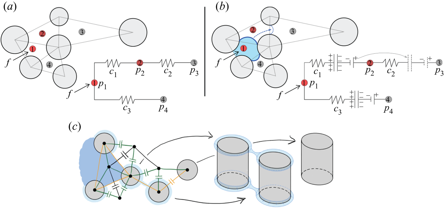
Each mesh triangle represents a pore (figure 2a), so we can build the pore-network incidence matrix (Strang Reference Strang2007) by examining the adjacency of the triangles. We number all pores and adopt the convention that pore connections are oriented in the direction of increasing pore number. As such, the incidence matrix of the network presented in figure 2(a) is
 \begin{equation} \boldsymbol{A} = \begin{bmatrix} -1 & 1 & 0 & 0 \\ 0 & -1 & 1 & 0 \\ -1 & 0 & 0 & 1 \end{bmatrix}, \end{equation}
where rows and columns of  $\boldsymbol {A}$ represent edges and nodes, respectively. Here, 1 and
 $-1$ indicate entering and leaving the node, respectively. For example, edge
 $1$ in (2.1) is directed from node
 $1$ to node
 $2$.
Schematic of flow through a porous medium and the analogue electrical circuit for (a) single-phase flow and (b) two-phase flow. Nodes of the electrical circuit correspond to pore centres. Viscous pressure drop is analogous to potential drop through resistors, and fluid–fluid interfaces are analogous to a combination of a capacitor and a battery. (c) Schematic of the dynamic pore-network model in strong imbibition ( $\theta <45^{\circ }$), where capacitors are placed at the fluid–fluid interfaces. Nodes are placed at pore and post centres; black, orange and green edges correspond to pore-to-pore, post-to-post and pore-to-post edges, respectively.

We also make use of the diagonal conductance matrix  $\boldsymbol {C}$, whose elements are the hydraulic conductivities of the network edges. The elements of
 $\boldsymbol {C}$ can be calculated as
 $c = {\rm \pi}r^{4}/8 \mu L$, assuming fully developed Hagen–Poiseuille flow through a rectangular tube with hydraulic radius
 $r$ and length
 $L$, which corresponds to pore-throat radius and the distance between pore centres in a micromodel geometry, respectively.
2.2. Single-phase flow
The difference in potential across the network edges can be obtained from the incidence matrix as  $\boldsymbol {e}=-\boldsymbol {A}\boldsymbol {p}$ (Strang Reference Strang2007). Here,
 $\boldsymbol {p}$ is an array of node potentials, which in the example of figure 2(a) would read as
 $\boldsymbol {p} = (p_1,p_2,p_3,p_4)^\textrm {T}$. The network currents can be calculated from the potential difference as
 $\boldsymbol {q}=\boldsymbol {C}\boldsymbol {e}$, where the example of figure 2(a) would have
 $\boldsymbol {q} = (q_1,q_2,q_3)^\textrm {T}$ and
 \begin{equation} \boldsymbol{C} = \begin{bmatrix} c_1 & 0 & 0 \\ 0 & c_2 & 0 \\ 0 & 0 & c_3 \end{bmatrix}. \end{equation}
At the same time, currents must obey Kirchhoff's current law (or mass conservation in fluid flow),  $\boldsymbol {A}^{T}\boldsymbol {q}=\boldsymbol {f}$, where
 $\boldsymbol {f}$ is the array of current sources at the nodes, and would read
 $\boldsymbol {f} = (f, 0, 0, 0)^\textrm {T}$ for the example in figure 2(a). After eliminating
 $\boldsymbol {e}$, single-phase flow through the network is captured by the following system of equations:
 $$\begin{gather} \boldsymbol{q}={-}\boldsymbol{C}\boldsymbol{Ap}, \end{gather}$$
 $$\begin{gather}\boldsymbol{A}^{T}\boldsymbol{q}=\boldsymbol{f}. \end{gather}$$
Eliminating  $\boldsymbol {q}$, the node potentials are given by
 \begin{equation} \boldsymbol{p}={-}(\boldsymbol{A}^{T}\boldsymbol{CA})^{{-}1}\boldsymbol{f}. \end{equation}
We set constant-flow boundary conditions at the inlet pores (at the centre of the flow cell) and zero-pressure boundary conditions at the outlet pores (at the edges of the flow cell).
2.3. Two-phase flow: moving capacitors
To extend the model to two-phase flow, we take advantage of the analogy between a capacitor and a fluid–fluid interface, where the drop in potential across the capacitor plates is analogous to the Laplace pressure. Consider the network diagram in figure 2(b). Initially, the capacitor is between nodes 1 and 2. As the current flows through the network, the capacitor accumulates charge and the potential difference across its plates builds. Capacitors with high accumulated potential difference hinder further flow, redirecting it elsewhere. Once the capacitor is filled to its maximum capacity, we allow it to advance to the next stable configuration at the neighbouring edges (between nodes 2 and 3).
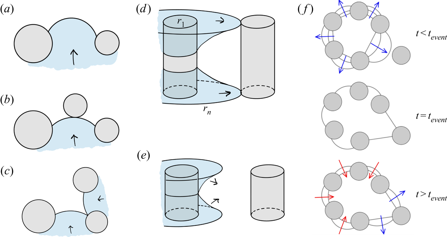
Our previous work on quasi-static fluid–fluid displacement (Primkulov et al. Reference Primkulov, Talman, Khaleghi, Rangriz Shokri, Chalaturnyk, Zhao, MacMinn and Juanes2018) provides a framework for deciding how and when capacitors move. For any given configuration of the fluid–fluid interface (capacitor locations), the quasi-static model predicts both the critical Laplace pressures ( $\Delta {p_{{crit}}}$) and the type of interface instability. The type of instability event (i.e. burst, touch, overlap or corner flow; see figure 3) determines the next stable interface configuration (Cieplak & Robbins Reference Cieplak and Robbins1988, Reference Cieplak and Robbins1990; Primkulov et al. Reference Primkulov, Talman, Khaleghi, Rangriz Shokri, Chalaturnyk, Zhao, MacMinn and Juanes2018). The critical Laplace pressure for burst, touch and overlap events can be written as
 \begin{equation} \Delta{p_{{crit}}} = \gamma \left(\frac{1}{r_{in}} + \frac{1}{r_{out}}\right), \end{equation}
where  $1/r_{out} = 2\cos \theta /h$ is the out-of-plane curvature of the fluid–fluid interface and
 $1/r_{in}$ is the in-plane curvature that corresponds to either burst, touch or overlap configurations (figure 3a–c). Burst events correspond to the highest stable in-plane curvature of the interface between two posts (figure 3a). Touch events correspond to the interface coming in contact with a nearby post (figure 3b). Overlap events occur when two neighbouring interfaces coalesce within the pore space (figure 3c). When
 $\theta <45^{\circ }$, the invading fluid tends to coat the corners between the posts and top/bottom plates. Corner-flow events occur when the horizontal extent of such meniscus reaches the nearest uncoated post (figure 3d). If these corner menisci instead overlap midpost, they form a capillary bridge that expands spontaneously to the nearest post (figure 3e). The value of
 $\Delta {p_{{crit}}}$ for corner flow and capillary bridge events is calculated from the total curvature of the meniscus configurations depicted in figure 3(d,e). A more detailed description of all pore-scale events is given in Primkulov et al. (Reference Primkulov, Talman, Khaleghi, Rangriz Shokri, Chalaturnyk, Zhao, MacMinn and Juanes2018).
(a) A burst event occurs when the interface pushes past its highest stable curvature. (b) A touch event occurs when the interface touches the post ahead. (c) An overlap event occurs when two neighbouring interfaces touch and coalesce, filling the pore cooperatively. (d) A corner-flow event occurs when a corner meniscus touches and coats the neighbouring post. (e) A capillary-bridge event occurs when corner menisci coalesce midpost before reaching the next post. (f) A sequence of interface configurations before and after pore-invasion event at  $t=t_{event}$ in capillary-dominated displacement. Figure adapted from Primkulov et al. (Reference Primkulov, Talman, Khaleghi, Rangriz Shokri, Chalaturnyk, Zhao, MacMinn and Juanes2018).

We assume that the pressure drop across a capacitor at time  $t$ can be written as
 $\Delta {p_{{crit}}} \varPhi (t) + \Delta {p_{{min}}}(1-\varPhi (t))$, where the filling ratio
 $\varPhi (t)$ measures the fraction of the throat filled with invading fluid (Holtzman & Segre Reference Holtzman and Segre2015). A throat volume is defined as
 $2r L h$. We chose
 $\Delta {p_{{min}}}$ so that it is equal to the smallest value of
 $\Delta {p_{{crit}}}$ minus the standard deviation of
 $\Delta {p_{{crit}}}$ within the network. This choice ensures that all menisci have the same Laplace pressure when corresponding throats are empty. Taking into account the direction of the edges (an array
 $\boldsymbol {d}(t)$ consisting of
 $1$ and
 $-1$ for edges directed towards and away from the defending fluid, respectively), the total pressure drop across the network edges can be written as
 $\boldsymbol {e} = \boldsymbol {b} - \boldsymbol {Ap}$, where non-zero components of pressure drop array
 $\boldsymbol {b}(t)$ are written as
 $-\boldsymbol {d}(t)[\Delta {p_{{crit}}} \varPhi (t) + \Delta {p_{{min}}}(1-\varPhi (t))]$. Therefore, the equations governing two-phase flow through the network are
 \begin{equation} \begin{bmatrix} \boldsymbol{C}^{{-}1}(t) & \boldsymbol{A} \\ \boldsymbol{A}^{T} & \boldsymbol{0} \end{bmatrix} \begin{bmatrix} \boldsymbol{q}(t) \\ \boldsymbol{p}(t) \end{bmatrix} = \begin{bmatrix} \boldsymbol{b}(t)\\ \boldsymbol{f} \end{bmatrix}. \end{equation}
We now discuss the time-stepping method in our two-phase flow model. After we initialize the interface locations within the ‘circuit’, we use adaptive forward Euler time-stepping to update the filling ratios of the network edges at the interface,  $\varPhi (t)$. We ensure that no pore throat is filled in a single time step (Aker et al. Reference Aker, Måløy, Hansen and Batrouni1998). After every time step, we use the effective viscosity (Aker et al. Reference Aker, Måløy, Hansen and Batrouni1998; Holtzman & Segre Reference Holtzman and Segre2015)
 $\mu = \mu _i \varPhi (t)+\mu _d(1-\varPhi (t))$ to update the conductivity matrix
 $\boldsymbol {C}(t)$ and resolve the flow via (2.7) with updated pressure drops across capacitors.
Whenever we encounter a time step ( $\Delta {t}$) where one of the components of
 $\varPhi (t)$ is greater than one, we repeat the time step with an adjusted
 $\Delta {t}$ until the unstable edge is exactly filled. Then, we remove the filled capacitor and replace it with empty capacitors at locations based on the type of instability that the quasi-static model outputs for the corresponding network edge (Primkulov et al. Reference Primkulov, Talman, Khaleghi, Rangriz Shokri, Chalaturnyk, Zhao, MacMinn and Juanes2018). Newly added capacitors are initialized with
 $\varPhi =0$ and accumulate potential drop as the above steps are repeated.
The typical solution of (2.7) in capillary-dominated regime produces the invasion sequence depicted in figure 3(f), which can be separated into three steps: (i) interface curvatures build slowly across the displacement front ( $t< t_{event}$); (ii) one of the interfaces reaches a ‘burst’, ‘touch’ or ‘overlap’ configuration, and the corresponding pore is instantaneously invaded with new interfaces having zero in-plane curvature and
 $\varPhi$ (
 $t=t_{event}$); and (iii) the invading fluid redistributes to equalize the Laplace pressures at the displacement front (
 $t>t_{event}$). The displacement front spends the majority of its time in step (i). Since capturing the short-time dynamics of invasion events (e.g. Haines Reference Haines1930) was not the primary objective of this work, we chose to make step (ii) instantaneous, and chose a relatively coarse
 $\Delta {t}$, with (iii) taking up only a few time steps between pore-invasion events. As a result, having
 $\varPhi =0$ correspond to zero in-plane curvature (our model) and having
 $\varPhi =0$ correspond to a negative in-plane curvature (expected experimentally) would only make an appreciable difference in the short-time-scale dynamics, which is outside the scope of interest of this study. Indeed, it is likely that a fully resolved model of the interface at the pore level is needed to capture these short-time-scale dynamics.
While our model of two-phase flow allows for re-emptying of network edges at the interface (figure 3f), our current implementation prohibits instability events in the reverse direction for simplicity of bookkeeping.
2.4. Moving-capacitor model in strong imbibition
When  $\theta <45^{\circ }$, the total curvature of a corner meniscus (figure 3d,e) can be negative. This means that at some
 $\theta <45^{\circ }$, invading fluid may advance by coating post corners instead of filling pore volumes. This was demonstrated in the strong imbibition experiments of Zhao et al. (Reference Zhao, MacMinn and Juanes2016). Our treatment of strong imbibition fits naturally into the two-phase model described above, where the lowest
 $\Delta {p_{crit}}$ corresponds to either corner flow (figure 3d) or a capillary bridge event (figure 3e). Below, we highlight a few distinguishing features of the ‘moving capacitor’ model for
 $\theta <45^{\circ }$.
The overall flow network accounts for three distinct components: (i) a pore network, where nodes are pore centres and edges are pore-to-pore channels (black network in figure 2c); (ii) a post corner network, where nodes are placed at the centres of posts and edges are post-to-post connections (orange network in figure 2c); and (iii) a network connecting post centres to pore centres (green network in figure 2c).
Hydraulic radii of post-to-post and pore-to-post connections are taken as twice the ratio of channel cross-sectional area to its wetted perimeter, which are calculated from the shape of the corner meniscus at its critical Laplace pressure (figure 3d,e). Volume assigned to a corner meniscus is defined to be  $2{\rm \pi} r_{post} {\rm \pi}r_{hydr}^{2}$, where
 $r_{post}$ and
 $r_{hydr}$ are radius of the post and hydraulic radius of the meniscus, respectively.
In post-to-post and pore-to-post capacitors, the value of  $\varPhi$ is assigned to a post, so that capacitors belonging to the same post have identical Laplace pressures at any given time. When a new post is coated, only one capacitor is removed from the network, the capacitor at the post-to-post connection (figure 2c), and new capacitors are added at the fluid–fluid boundaries of the new post.
Another distinction between the model we present here from the original ‘moving capacitor’ model is that the corner events depicted in figure 3(d,e) can trigger pore invasion. The volume of each pore in our network is bounded by three posts. Therefore, if all three posts experience corner events, the oil phase within the pore space pinches off and pore gets filled with invading fluid (Odier et al. Reference Odier, Levaché, Santanach-Carreras and Bartolo2017).
Finally, our model assumes perfectly smooth surfaces and leaves out the role that surface roughness, dynamic contact angle and potential precursor films may play in the fluid–fluid displacement experiments. While our model on this idealized substrate predicts no corner flow when  $h=100\ \mathrm {\mu }\textrm {m}$ (Primkulov et al. Reference Primkulov, Talman, Khaleghi, Rangriz Shokri, Chalaturnyk, Zhao, MacMinn and Juanes2018), experiments detect the onset of corner flow for
 $\theta$ somewhere between
 $7^{\circ }$ and
 $60^{\circ }$ (Zhao et al. Reference Zhao, MacMinn and Juanes2016). This discrepancy between experiment and the model is reconciled through a fitting parameter that we discuss in detail in Appendix A.
3. Principal flow regimes
We begin our discussion by exploring the five principal regimes of fluid–fluid displacement in porous media: (i) viscous fingering; (ii) stable displacement; (iii) invasion percolation; (iv) cooperative pore filling; and (v) corner flow. We anchor our discussion of principal flow regimes around a few key metrics that help to characterize and distinguish the regimes.
(i) Fractal dimension
 $D_f$ is a measure of how a pattern fills the space in which it is embedded. For a 2-D pattern, $D_f$ varies between 1 (for a line) and 2 (for a compact object). We calculate $D_f$ with the box-counting method (Kenkel & Walker Reference Kenkel and Walker1996). Following this method, we tile our flow patterns with boxes of size $\epsilon$ and count the number of boxes $N$ of that size needed to cover the pattern. We repeat this process for a sequence of $\epsilon$ and take $D_f$ to be the slope of $N$ against $\epsilon$ on a log–log plot (see Primkulov et al. (Reference Primkulov, Talman, Khaleghi, Rangriz Shokri, Chalaturnyk, Zhao, MacMinn and Juanes2018) for more details).
(ii) Finger width
$w/a$ is the ratio of mean finger width to mean pore size. We estimate $w/a$ following a scheme detailed in Primkulov et al. (Reference Primkulov, Talman, Khaleghi, Rangriz Shokri, Chalaturnyk, Zhao, MacMinn and Juanes2018), which is an adaptation of an approach by Cieplak & Robbins (Reference Cieplak and Robbins1988, Reference Cieplak and Robbins1990). Briefly, we divide our images into slices and record the mean size $w$ of one-dimensional clusters containing the pattern. We repeat the same process for an image where we treat the entire pore space as a pattern and record the mean pore throat size as $a$.(iii) Modified capillary number (
${Ca}^{*}$) measures the fraction of characteristic viscous to capillary pressures in our setup. We take
(3.1)after expanding the characteristic pressure drop as\begin{equation} {Ca}^{*} = \frac{\Delta p_{visc}}{\Delta p_{cap}} = \frac{\max({Ca},{Ca}/M)}{|\Delta p_{crit}|}\frac{\gamma R}{a h}, \end{equation}$\Delta p_{visc} = \max (\mu _i,\mu _d) u R /ah$, where $R$ is the radius of the Hele-Shaw cell. The term $\max ({Ca},{Ca}/M)$ ensures that the greater viscous forces are taken into account, and the magnitude of critical Laplace pressure $|\Delta p_{crit}|$ is taken directly from simulations.


All of these metrics are time dependent. We evaluate  $D_f$ and
 $w/a$ at the moment of breakthrough, when the invading fluid first reaches the outer boundary of the flow cell. The characteristic velocity
 $u$ used in calculating
 ${Ca}$ and
 ${Ca}^{*}$ is taken as
 $Q/2{\rm \pi} r_{min}$, where
 $r_{min}$ is the radial distance of the post closest to centre of the Hele-Shaw cell. Additionally, we define a directional flow rate as the mean flow rate along different directions of the radial flow cell. We do so by dividing the flow cell into
 $10^{\circ }$ sectors and calculating the mean flow rate for each sector as time progresses.
3.1. Stable displacement ($D_f=1.93$, $w/a=37$, ${Ca}^{*}>1$)


When a more viscous fluid displaces a less viscous fluid ( $M>1$), the displacement front is hydrodynamically stable (Saffman & Taylor Reference Saffman and Taylor1958) because viscous forces smooth perturbations.
Simulations at  $M=10^{3}$,
 ${Ca}=10^{-1}$,
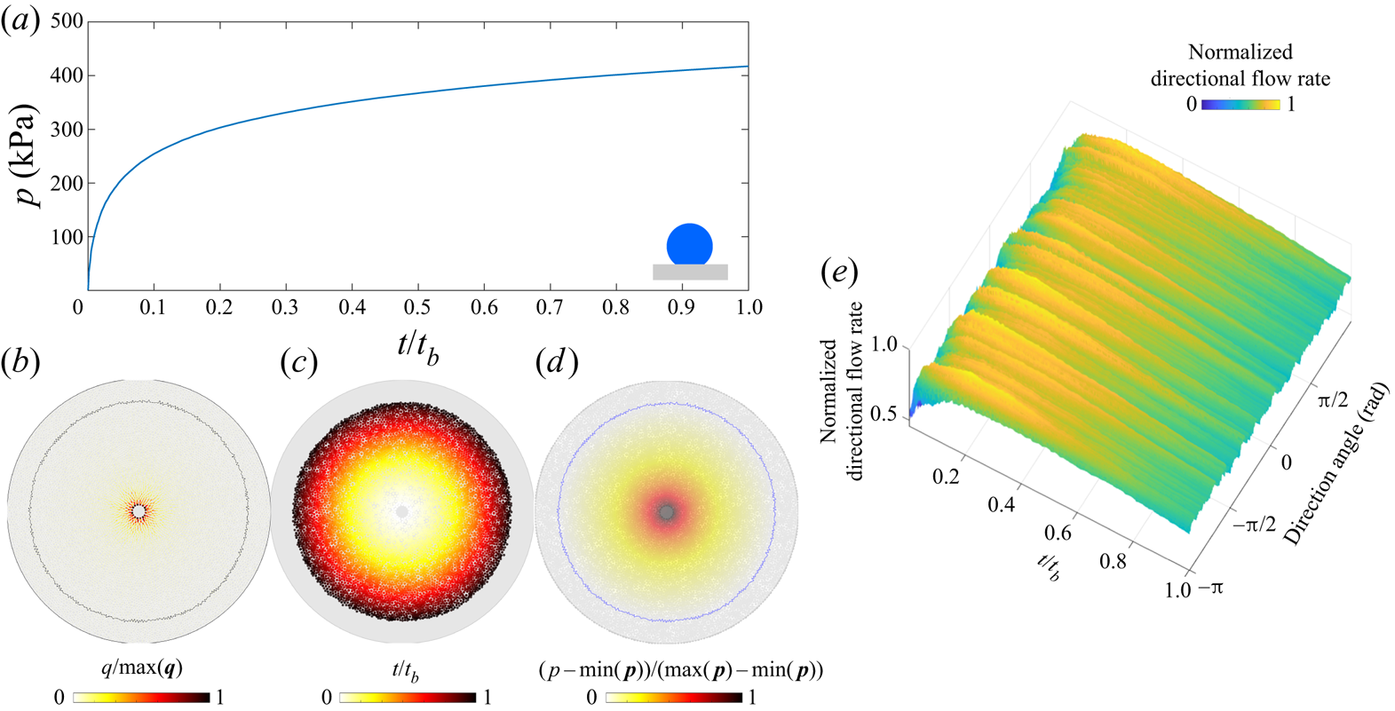
 $\theta \in [46^{\circ },180^{\circ }]$ produce nearly perfectly circular patterns (figure 4). The injection pressure increases as the displacement progresses (figure 4a), with most of the pressure drop taking place in the invading fluid (figure 4d). The flow rate is radially symmetric, decreasing with radius (figure 4b,e) and pattern symmetry is maintained throughout (figure 4c).
Stable displacement in the benchmark geometry for  ${Ca}=10^{-1}$,
 $M=10^{3}$ and
 $\theta =170^{\circ }$: (a) the injection pressure increases monotonically (
 $t_b$ is the breakthrough time); (b) flow rates within the network show radial symmetry and radially decreasing intensity (
 $\max (\boldsymbol {q}$) is the largest local flow rate at given
 $t$); (c) pore-invasion times reflect the radial symmetry in pattern growth; (d) pore-pressure distribution, where pressure gradients are significant only in the invading fluid (
 $\max (\boldsymbol {p}$) is the largest local pressure at given
 $t$); and (e) the evolution of the directional flow rate is indicative of continuous compact flow, where apparent ridges are artefacts due to discrete pore throats with high flow rates near the cell centre.

3.2. Viscous fingering ($D_f=1.63$, $w/a=2.1$, ${Ca}^{*}>1$)


Stable displacement is often desirable, but not always attainable in industrial applications such as oil recovery (Chuoke et al. Reference Chuoke, van Meurs and van der Poel1959) and sugar processing (Hill Reference Hill1952). Viscous fingers develop under potential flow when a less-viscous fluid displaces a more viscous one ( $M<1$).
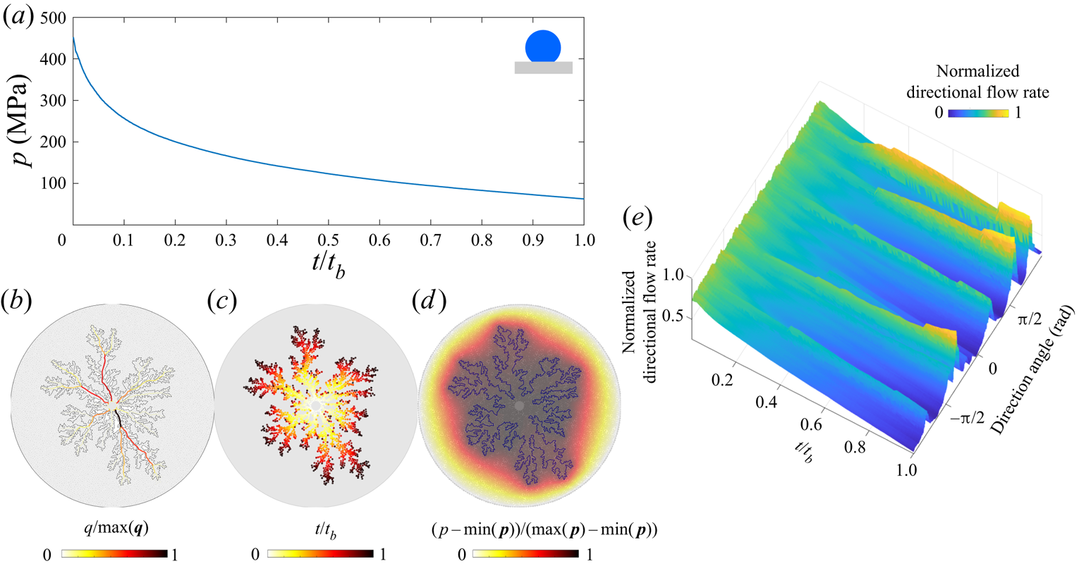
In figure 5, we highlight the signatures of viscous fingering for the benchmark pore geometry. The simulation in figure 5 is conducted for  ${Ca}=10^{-1}$,
 $M=10^{-3}$,
 $\theta =170^{\circ }$. As the displacement advances, the injection pressure decreases (figure 5a) because the majority of the pressure drop takes place in the defending fluid (figure 5d). Although the pressure appears to decrease smoothly in time, removing the global trend from the signal would expose fluctuations due to intermittent activity at the displacement front (Primkulov et al. Reference Primkulov, Pahlavan, Fu, Zhao, MacMinn and Juanes2019). As the fingers develop and grow, they focus the flow along their main branches (figure 5b,e). The displacement pattern remains radially symmetric throughout (figure 5c). In fact, the diffusive signature of the pressure field in the defending fluid is what generates the striking similarity between viscous fingering and other patterns in nature, such as diffusion-limited aggregation (known as DLA) (Meakin et al. Reference Meakin, Tolman and Blumen1989), dielectric breakdown of materials (Niemeyer, Pietronero & Wiesmann Reference Niemeyer, Pietronero and Wiesmann1984) and spreading of fire fronts (Conti & Marconi Reference Conti and Marconi2010). The diffusive pressure field arises from Darcy flow and incompressibility, which lead to
 $\nabla ^{2}p=0$ in the defending fluid, which is identical to the diffusive solute concentration field in diffusion-limited aggregation (Paterson Reference Paterson1984).
Viscous fingering in the benchmark geometry for  ${Ca}=10^{-1}$,
 $M=10^{-3}$ and
 $\theta =170^{\circ }$: (a) the injection pressure decreases monotonically in time (
 $t_b$ is the breakthrough time); (b) flow rates within the network are pronounced along the main branches of the viscous fingers (
 $\max (\boldsymbol {q}$) is the largest local flow rate at given
 $t$); (c) pore-invasion times reflect the radial symmetry in pattern growth; (d) pore-pressure distribution, where most pressure changes occur within the defending fluid (
 $\max (\boldsymbol {p}$) is the largest local pressure at given
 $t$); and (e) the evolution of the directional flow rate shows persistent (rather than sporadic) growth of viscous fingers.

3.3. Invasion percolation ($D_f=1.8$, $w/a=3$, ${Ca}^{*}<1$)


When the invading fluid advances very slowly and viscous forces are negligible ( ${Ca}\rightarrow 0$), the flow is governed exclusively by capillary forces. In drainage (
 $\theta >90^{\circ }$), the invading fluid advances mainly through burst events and the flow is well captured by the invasion percolation model (Chandler et al. Reference Chandler, Koplik, Lerman and Willemsen1982; Wilkinson & Willemsen Reference Wilkinson and Willemsen1983; Lenormand & Zarcone Reference Lenormand and Zarcone1985).
We explore the characteristics of invasion percolation by simulating fluid–fluid displacement at  ${Ca}=10^{-7}$,
 $M=1$, and
 $\theta =170^{\circ }$ on the benchmark pore geometry (figure 6). The pressure distribution in the invasion percolation regime is spatially uniform within each fluid (figure 6d), with the two fluid pressures differing by the Laplace pressure. As the displacement front advances, the pressure in the invading fluid is modulated by the sequence of lowest capillary entry pressures, and fluctuates sharply (figure 6a) (Måløy et al. Reference Måløy, Furuberg, Feder and Jøssang1992; Furuberg, Måløy & Feder Reference Furuberg, Måløy and Feder1996). This intermittency is also reflected in the flow field: only a small fraction of the pore space is active at any given time (figure 6b), and the flow direction changes frequently (figure 6e). As a result, the emerging flow pattern lacks radial symmetry throughout the displacement, with invasion-time patches reflecting invasion avalanches (figure 6c).
Invasion percolation in the benchmark geometry for  ${Ca}=10^{-7}$,
 $M=1$ and
 $\theta =170^{\circ }$: (a) the injection pressure fluctuates sharply due to pore-invasion events (
 $t_b$ is the breakthrough time); (b) flow rates within the network are very localized, only a small fraction of the pore space is hydrodynamically active at any given time (
 $\max (\boldsymbol {q}$) is the largest local flow rate at given
 $t$); (c) pore-invasion times show asymmetric pore invasion clusters; (d) the pore-pressure distribution is uniform within each fluid (
 $\max (\boldsymbol {p}$) is the largest local pressure at given
 $t$); and (e) the evolution of the directional flow rate shows intermittency in flow direction.

3.4. Cooperative pore filling ($D_f=1.93$, $w/a=15$, ${Ca}^{*}<1$)


Cooperative pore filling is a capillary-dominated regime that produces compact displacement patterns. Although cooperative pore filling can take place in viscous flow regimes, they are most prominent in weak imbibition and can dominate the displacement pattern when viscous forces are small. During cooperative pore filling, the displacement front advances mainly through overlap and touch events (see § 2), and the increased fraction of overlap events smoothens the displacement front (Cieplak & Robbins Reference Cieplak and Robbins1988, Reference Cieplak and Robbins1990; Holtzman & Segre Reference Holtzman and Segre2015; Primkulov et al. Reference Primkulov, Talman, Khaleghi, Rangriz Shokri, Chalaturnyk, Zhao, MacMinn and Juanes2018). As a result, the displacement front sweeps the defending fluid completely, producing compact displacement patterns (figure 7).
Cooperative pore filling in the benchmark geometry for  ${Ca}=10^{-7}$,
 $M=1$ and
 $\theta =46^{\circ }$: (a) the injection pressure is highly intermittent (
 $t_b$ is the breakthrough time); (b) flow rates within the network are localized, and only a small fraction of them have appreciable flow; (c) pore-invasion times reveal pore-invasion clusters (
 $\max (\boldsymbol {q}$) is the largest local flow rate at given
 $t$); (d) the pore-pressure distribution is uniform within each fluid phase (
 $\max (\boldsymbol {p}$) is the largest local pressure at given
 $t$); and (e) the evolution of the directional flow rate shows a high degree of intermittency in the flow direction.

Cooperative pore-filling simulations on the benchmark pore geometry at  ${Ca}=10^{-7}$,
 $M=1$ and
 $\theta =46^{\circ }$ (figure 7) show many similarities to invasion percolation (§ 3.3). The pressure is uniform in each fluid phase (figure 7d), but exhibits sharp fluctuations in time (figure 7a). The flow field is highly intermittent (figure 7e), with only a small fraction of pores active at any given moment (figure 7b). This intermittency results in asymmetric and patch-like growth of the displacement pattern (figure 7c). Unlike invasion percolation, cooperative pore filling produces compact displacement patterns with no trapped patches of defending fluid. The difference stems from the nature of pore-scale invasion events: invasion percolation is dominated by burst events while cooperative pore filling is dominated by overlap and touch events (Cieplak & Robbins Reference Cieplak and Robbins1988, Reference Cieplak and Robbins1990; Holtzman & Segre Reference Holtzman and Segre2015; Primkulov et al. Reference Primkulov, Talman, Khaleghi, Rangriz Shokri, Chalaturnyk, Zhao, MacMinn and Juanes2018).
3.5. Corner flow ($D_f=1.54$, $w/a=0.8$, ${Ca}^{*}<1$)


In strong imbibition, the invading fluid no longer advances by filling the pores completely – instead, the invading fluid advances mainly through corner-flow events where it coats the corners at the intersection of posts with the top and bottom plates of the Hele-Shaw cell (figure 2c).
Figure 8 explores corner flow through simulations at  ${Ca}=5 \times 10^{-7}$,
 $M=0.1$ and
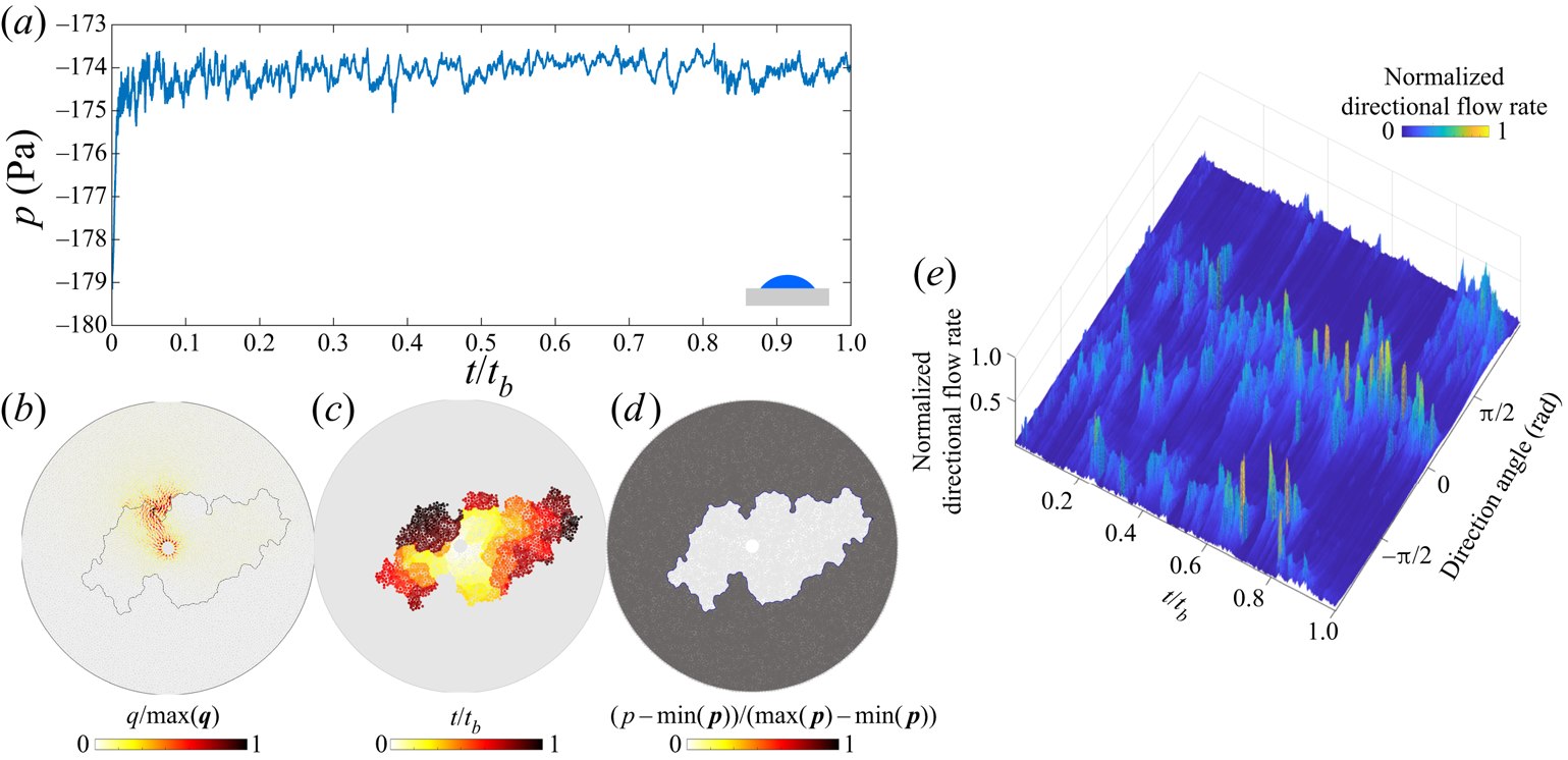
 $\theta =4^{\circ }$ on the benchmark pore geometry. Corner flow shares many similarities with other capillary-dominated regimes. The spatial distribution of pressure is uniform within each fluid (figure 8d), while the injection pressure shows intermittency characteristic of capillary-dominated displacements (figure 8a). Only a small fraction of the pore space has appreciable flow (figure 8b), and flow changes direction frequently (figure 8e). The resulting pattern grows asymmetrically throughout the displacement (figure 8c).
Corner flow in the benchmark geometry for  ${Ca}=5\times 10^{-7}$,
 $M=0.1$ and
 $\theta =4^{\circ }$: (a) the injection pressure is highly intermittent (
 $t_b$ is the breakthrough time); (b) flow rates within the network are localized, and only a small fraction of them have appreciable flow (
 $\max (\boldsymbol {q}$) is the largest local flow rate at given
 $t$); (c) pore-invasion times show radial asymmetry; (d) the pore-pressure distribution is uniform within each fluid phase (
 $\max (\boldsymbol {p}$) is the largest local pressure at given
 $t$); and (e) the evolution of the directional flow rate shows a high degree of intermittency in the flow direction.

4. Crossover from viscous-dominated to capillary-dominated flow
We examine the difference in the invasion dynamics between high and low  ${Ca}$ through the spatial and temporal distributions of pore-invasion events. In this section, we focus on unfavourable viscosity contrast displacement,
 $M=1/340$ (Zhao et al. Reference Zhao, MacMinn and Juanes2016, Reference Zhao2019). The effective ratio of viscous to capillary forces is therefore
 ${Ca}/M$, which we use in this section. Figure 9(a) shows histograms of the Euclidean distance
 $\Delta s$ between consecutive pore-invasion events. The distribution of
 $\Delta s$ indicates that consecutive pore-invasion events are significantly more likely to take place near each other for low
 ${Ca}/M$ than for high
 ${Ca}/M$. Furthermore, the time
 $\Delta t_{inv}$ between consecutive pore-invasion events at
 ${Ca}/M=10^{-7}$ shows that the median
 $\Delta t_{inv}$ increases as
 $\theta \rightarrow 46^{\circ }$ (figure 9b). As the wettability of the substrate changes from strong drainage to weak imbibition, the relative frequency of cooperative pore-filling events increases (Cieplak & Robbins Reference Cieplak and Robbins1990, Reference Cieplak and Robbins1988; Primkulov et al. Reference Primkulov, Talman, Khaleghi, Rangriz Shokri, Chalaturnyk, Zhao, MacMinn and Juanes2018). The increase in
 $\Delta t_{inv}$ is chiefly due to the increase in relative frequency of overlap events, which result in rapid invasion of several neighbouring pores. This in turn leads to significant retraction of the invading fluid from all of the throats at the displacement front. Thus, more time is needed to refill the pores at the displacement front, which results in the steady increase in
 $\Delta t_{inv}$ as
 $\theta$ decreases (figure 9b).
(a) Histogram of the distance ( $\Delta s$) between consecutive pore-invasion events. (b) Median time (
 $\Delta t_{inv}$) between consecutive pore-invasion events as a function of
 $\theta$. (c) Spatio-temporal autocorrelation of the normalized directional flow rate fields for
 $\theta =46^{\circ }$. (d–f) Temporal evolution of the normalized directional-flow-rate fields for
 $\theta =46^{\circ }$ and (d)
 ${Ca}/M = 10^{-3}$, (e)
 ${Ca}/M = 10^{-6}$, (f)
 ${Ca}/M = 10^{-7}$. The plots are complemented with the pore invasion time diagrams (insets).

The velocity distribution within the porous medium is also strikingly different at low and high  ${Ca}/M$. We plot the temporal evolution of the directional flow rate for
 $\theta =46^{\circ }$ in figure 9(d–f). At
 ${Ca}/M=10^{-3}$, the invading fluid forms high velocity flow channels that persist until breakthrough (figure 9d). The pressure gradients in the defending fluid dominate the dynamics, and the invading fluid flows through growing viscous fingers. The displacement front advances with strong radial symmetry (figure 9d), as observed experimentally (Måløy et al. Reference Måløy, Feder and Jøssang1985; Løvoll et al. Reference Løvoll, Méheust, Toussaint, Schmittbuhl and Måløy2004; Holtzman, Szulczewski & Juanes Reference Holtzman, Szulczewski and Juanes2012). As
 ${Ca}/M$ decreases (figure 9e,f), the front velocity becomes increasingly intermittent. The pressure gradients within the fluids are negligible, and the pressure changes in the network are due almost exclusively to the Laplace pressure at the displacement front. Only portions of the displacement front are active at any given time (Ferer et al. Reference Ferer, Ji, Bromhal, Cook, Ahmadi and Smith2004; Holtzman et al. Reference Holtzman, Szulczewski and Juanes2012), and the front advances in asymmetric patches (figure 9e,f).
This transition from viscous-dominated to capillary-dominated flow can be quantified through the spatio-temporal autocorrelation of the normalized directional flow rate (figure 9c). The autocorrelation is calculated as  $C(\alpha ,\tau )={\langle q(\alpha ,t)q(\alpha ,t+\tau ) \rangle }/\langle q(\alpha ,t) q(\alpha ,t) \rangle$, where
 $\langle \cdot \rangle$ indicates the ensemble average over time,
 $\alpha$ is the direction and
 $\tau$ is the time separation between the directional flow rate profiles. The average of
 $C(\alpha ,\tau )$ over all
 $\alpha$ is shown in figure 9(c) for
 $\theta =46^{\circ }$. The flow field becomes increasingly uncorrelated at low
 ${Ca}/M$, with a qualitative transition taking place below
 ${Ca}/M=10^{-5}$.
5. Extending Lenormand's phase diagram
We extend Lenormand's diagram by simulating fluid–fluid displacement over a wide range of  $\theta$,
 ${Ca}$,
 $M$ on the benchmark pore geometry (7560 simulations in total). This thorough sweep of the parameter space is possible due to the relatively low computational cost of our model. For each simulation, we measure
 $D_f$,
 $w/a$ and
 ${Ca}^{*}$ at the moment of breakthrough. We use these variables to delineate regions corresponding to the different principal flow regimes.
First, we use the fractal dimension  $D_f$ to separate compact patterns from non-compact patterns. Compact patterns include stable displacement and cooperative pore filling, both of which have
 $D_f>1.92$ (maroon isosurface in figure 10d). A threshold based on
 $w/a$ provides similar results (not shown).
Evolution of  $D_f$ in
 $M$–
 ${Ca}$–
 $\theta$ space. Slices of the simulation data in (a) drainage, (b) weak imbibition and (c) strong imbibition. (d) The maroon isosurface corresponding to
 $D_f=1.92$ is used to draw the boundary between compact and non-compact displacement patterns. The black lines are the intersections of the isosurface with the cross-sections.

Next, we use  ${Ca}^{*}$ to separate viscous-dominated flow regions (stable displacement and viscous fingering) from capillary-dominated flow regions (cooperative pore filling, invasion percolation and corner flow). The surface resulting from
 ${Ca}^{*} = 1$ in (3.1) is depicted in figure 11 in dark grey: the space above this surface is viscous-dominated, the space below it is capillary-dominated. The crease on the
 ${Ca}^{*} = 1$ surface originates from a vanishing out-of-plane contribution to Laplace pressure near
 $\theta =90^{\circ }$.
Viscous-dominated and capillary-dominated regions of  $M$–
 ${Ca}$–
 $\theta$ space are separated by setting
 ${Ca}^{*} = 1$ in (3.1). This is depicted with a dark grey surface in this figure.

The combination of the maroon and grey isosurfaces from figures 10 and 11 is sufficient for delineating the principal flow regimes as follows.
(i) Invasion percolation is capillary dominated (
${Ca}^{*}<1$) and non-compact ($D_f<1.92$).(ii) Cooperative pore filling is capillary dominated (
${Ca}^{*}<1$) and compact ($D_f>1.92$).(iii) Corner flow is capillary dominated (
${Ca}^{*}<1$) and non-compact ($D_f<1.92$).(iv) Viscous fingering is viscous dominated (
${Ca}^{*}>1$) and non-compact ($D_f<1.92$).(v) Stable displacement is viscous dominated (
${Ca}^{*}>1$) and compact ($D_f>1.92$).


Although we use sharp boundaries to outline regions that belong to different flow regimes, the transitions from one regime to another are smooth, as is evident from the cross-section images in figures 10 and 11.
Our extension of Lenormand's diagram with added wettability axis is presented in figure 12. Our model faithfully reproduces the original diagram in drainage (cross-section  $\theta =180^{\circ }$ in figure 12), but reveals a more complete picture of the fluid–fluid displacement in porous media by augmenting the phase diagram with a wettability (
 $\theta$) axis.
Extended Lenormand diagram constructed using  ${Ca}^{*}$ and
 $D_f$ phase boundaries from figures 10 and 11 to separate the five principal flow regimes within the
 $M$–
 ${Ca}$–
 $\theta$ parameter space: viscous fingering, stable displacement, invasion percolation and cooperative pore filling. Results from the ‘moving capacitor’ model are complemented with results from the quasi-static model that allows inferring the extent of cooperative pore filling in the limit
 ${Ca}\rightarrow 0$.

To assess the influence of pore-scale disorder on the displacement pattern, we run simulations on a pore geometry in which we can precisely define, and tune, the degree of geometric variability among realizations. To do so, we generate a regular triangular lattice with 2.8 mm spacing between vertices and place posts on its vertices. The radii of the posts are drawn from a uniform distribution  $(r_0-\xi r_v,r_0+\xi r_v)$, where
 $r_0=1100\ \mathrm {\mu }\textrm {m}$ and
 $r_v=300\ \mathrm {\mu }\textrm {m}$ are selected to match the mean post size of the benchmark geometry and
 $\xi \in [0,1]$ is the index of disorder. When
 $\xi =0$, the medium is ordered and anisotropic; when
 $\xi =1$, the medium is disordered and isotropic. As demonstrated in Appendix B, the values of
 $D_f$ and
 $w/a$ do not change significantly with the degree of disorder
 $\xi$. Therefore, although the data in figure 12 were collected from simulations on a single benchmark pore geometry, the results apply generally to porous media with varying degree of disorder. The capillary-dominated region of the phase diagram (
 ${Ca}^{*}<1$) is divided into invasion percolation, cooperative pore filling and corner flow. The boundary between compact and non-compact flow in the capillary-dominated region of figure 12 changes significantly with
 ${Ca}$: the upper and lower bounds (in
 $\theta$) of the cooperative pore filling region move apart as
 ${Ca}$ approaches the grey surface. When
 $M>1$, viscous forces stabilize the displacement front and aid cooperative pore filling events in making the patterns more compact (Hu et al. Reference Hu, Wan, Yang, Chen and Tokunaga2018).
The shape of the extended Lenormand diagram can be inferred outside the  $M$–
 ${Ca}$–
 $\theta$ parameter space probed with the ‘moving capacitor’ model in figure 12. In particular, the cooperative pore filling region extends farther into the
 $M<1$ region as
 ${Ca}$ decreases. This is evident from the quasi-static limit of the model, where cooperative pore filling boundaries are independent of
 $M$.
The extended Lenormand diagram in figure 12 is generated for a single pore geometry. While the overall shape of the diagram is expected to hold across different micromodels with a wide range of pore-scale disorder, spacing between the posts and gap thickness  $h$, the boundaries between the principal flow regimes are likely to shift depending on the pore structure. For example, increasing the spacing between the post centres would bring the onset of cooperative pore filling to higher
 $\theta$ (Primkulov et al. Reference Primkulov, Talman, Khaleghi, Rangriz Shokri, Chalaturnyk, Zhao, MacMinn and Juanes2018). Larger spacing between the posts would also make corner flow less dominant in strong imbibition, as higher critical pressures would be needed to coat post corners. Therefore, compact displacement would occupy a greater proportion of the overall space in figure 12. The degree of disorder is also known to roughen the displacement front and shift the boundary between invasion percolation and viscous fingering (Holtzman & Juanes Reference Holtzman and Juanes2010; Holtzman Reference Holtzman2016; Hu et al. Reference Hu, Lan, Wei and Chen2019). Given that the pore geometry used in figure 12 is similar to one with
 $\xi =0.99$ in Appendix B, a pore space with smaller degree of disorder would make compact displacement more favourable, which in turn would enlarge the compact displacement region in figure 12 (stable displacement and cooperative pore filling).
One should not think of the boundaries between the principal flow regimes in figure 12 as sharp, because transitions from one regime to another are gradual. Regions of the  $M$–
 $\theta$–
 ${Ca}$ space near the maroon and grey boundaries correspond to crossover zones between principal flow regimes.
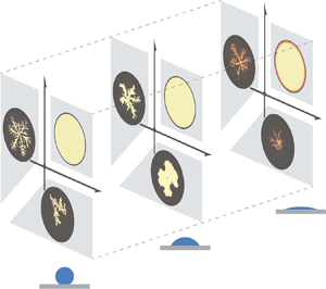
We summarize the findings from our comprehensive study with a schematic (figure 13). The classic phase diagram of Lenormand was developed for strong drainage (figure 13a), where displacement patterns advance through either viscous fingering, stable displacement or invasion percolation. This diagram undergoes a qualitative change when the system moves to weak imbibition (figure 13b), in which viscous fingers become significantly wider and invasion percolation is replaced by cooperative pore filling. Therefore, the majority of the  $M$–
 ${Ca}$ space leads to compact displacement patterns. Strong imbibition has only been sparsely studied (Zhao et al. Reference Zhao, MacMinn and Juanes2016; Odier et al. Reference Odier, Levaché, Santanach-Carreras and Bartolo2017; Primkulov et al. Reference Primkulov, Talman, Khaleghi, Rangriz Shokri, Chalaturnyk, Zhao, MacMinn and Juanes2018), but enough is known to outline the main modes of displacement (figure 13c). The displacement patterns advance through corner flow at low
 ${Ca}$, where the injected fluid occupies only a fraction of the pore space (denoted by darker shades in figure 13c). This mode of displacement has been explored experimentally by Zhao et al. (Reference Zhao, MacMinn and Juanes2016) and Odier et al. (Reference Odier, Levaché, Santanach-Carreras and Bartolo2017), and numerically in the quasi-static limit (Primkulov et al. Reference Primkulov, Talman, Khaleghi, Rangriz Shokri, Chalaturnyk, Zhao, MacMinn and Juanes2018). The invasion pattern advances through thin films on the solid surface for high
 ${Ca}$ and
 $M<1$ (Levaché & Bartolo Reference Levaché and Bartolo2014), while maintaining the viscous fingering morphology (Zhao et al. Reference Zhao, MacMinn and Juanes2016).
A sketch of Lenormand's phase diagram in (a) strong drainage, (b) weak imbibition and (c) strong imbibition. The darker shades in strong imbibition represent partial pore-scale displacement. Art credit: Kamilla Omarova.

The simulations in figure 12 reproduce many experimental observations. First, as  $\theta$ changes from
 $180^{\circ }$ to
 $46^{\circ }$, displacement patterns change from invasion percolation to cooperative pore filling (Trojer et al. Reference Trojer, Szulczewski and Juanes2015; Zhao et al. Reference Zhao, MacMinn and Juanes2016), and finger width increases in the viscous-fingering region of the diagram (Stokes et al. Reference Stokes, Weitz, Gollub, Dougherty, Robbins, Chaikin and Lindsay1986; Trojer et al. Reference Trojer, Szulczewski and Juanes2015; Zhao et al. Reference Zhao, MacMinn and Juanes2016). Second, the injection pressure fluctuates sharply in capillary-dominated regimes (Måløy et al. Reference Måløy, Furuberg, Feder and Jøssang1992; Furuberg et al. Reference Furuberg, Måløy and Feder1996), but instead varies monotonically with time in viscous-dominated regimes. Third, the model naturally reproduces the intermittent flow that is modulated by pore disorder in capillary-dominated flow. Finally, the model reproduces the interplay between imposed ordered post lattice and the flow morphology: snow flake patterns in viscous fingering (Chen & Wilkinson Reference Chen and Wilkinson1985; Chen Reference Chen1987), regular crystal-growth morphology in cooperative pore filling regime (Lenormand Reference Lenormand1990), perfect circles in stable displacement and disordered morphology in invasion percolation (Wilkinson & Willemsen Reference Wilkinson and Willemsen1983; Lenormand & Zarcone Reference Lenormand and Zarcone1985; Måløy et al. Reference Måløy, Furuberg, Feder and Jøssang1992).
While our ‘moving capacitor’ model is successful in reproducing the dynamics of the principal flow regimes (figure 13), it assumes piston-like displacement for burst, touch and overlap events. As a result, the model overestimates the invading fluid saturation at high  ${Ca}$, as pointed out by Zhao et al. (Reference Zhao2019). Strong drainage and high
 ${Ca}$ features residual films of defending fluid (Bretherton Reference Bretherton1961; Zhao et al. Reference Zhao, MacMinn and Juanes2016). In strong imbibition, invading fluid films dominate the displacement patterns in viscous fingering and corner flow regimes (Levaché & Bartolo Reference Levaché and Bartolo2014; Zhao et al. Reference Zhao, MacMinn and Juanes2016; Odier et al. Reference Odier, Levaché, Santanach-Carreras and Bartolo2017). These regimes are captured more naturally through pore-scale 3-D continuum models (Zhao et al. Reference Zhao2019), which are unfortunately still prohibitively expensive for populating significant portions of the
 $M$–
 ${Ca}$–
 $\theta$ parameter space in Lenormand's diagram (figure 12).
6. Conclusion
We have presented the results of a ‘moving capacitor’ dynamic pore-network model that is able to reproduce the full  $M$–
 ${Ca}$ space of Lenormand's phase diagram and extend it with a third dimension
 $\theta$, thus accounting for the system's wettability. The model captures the pressure and flow within the porous medium, and our analysis of the model results shows the contrast in pore-scale dynamics between viscous-dominated and capillary-dominated flow through pore-invasion-event statistics and autocorrelation of the velocity field. The ‘moving capacitor’ model provides a single framework that captures the dynamics of fluid–fluid displacement in micromodels across an unprecedented span of
 $M$–
 ${Ca}$–
 $\theta$ parameters. The model cannot be directly applied to generic porous materials with complex shapes or hierarchical geometries. However, in the spirit of Lenormand et al. (Reference Lenormand, Touboul and Zarcone1988) and Cieplak & Robbins (Reference Cieplak and Robbins1988), here we studied a simpler pore geometry in order to learn something general about two-phase displacement in more complex porous media. We use our model to build the first 3-D version of Lenormand's phase diagram with wettability as the third axis, whose general shape we expect to hold for more complex 3-D porous materials. We demonstrate that cooperative pore filling can occupy a significant portion of
 $M$–
 ${Ca}$–
 $\theta$ space, and that two metrics – the classical fractal dimension and modified capillary number
 ${Ca}^{*}$ – are sufficient for delineating the five principal displacement regimes. One can use the diagram to design efficient fluid–fluid displacement in disordered porous media. Furthermore, the ‘moving capacitor’ model used in this work enables modelling multiphase flow in deformable granular media (movable posts) (Jain & Juanes Reference Jain and Juanes2009; Sandnes et al. Reference Sandnes, Flekkøy, Knudsen, Måløy and See2011; Lee et al. Reference Lee, Lee, Le Mestre, Xu and MacMinn2020), while accounting for the wettability effects, when combined with discrete element method (known as DEM) models (Meng et al. Reference Meng, Primkulov, Yang, Kwok and Juanes2020).
Acknowledgements
The authors would like to thank A. Jacquey, E. Haghighat, J.A. da Silva Jr., W. Li, J. Li and P. Mora for insightful discussions and help with computation during the project.
Funding
This work was funded by the KFUPM-MIT collaborative agreement ‘Multiscale Reservoir Science’. R.J. acknowledges funding from the US Department of Energy (grant DE-SC0018357).
Declaration of interests
The authors declare no conflict of interest.
Appendix A. Fitting parameter for corner flow
A.1. Ideal system
We first highlight how changes in  $h$ – the height of posts within our micromodel – impact the onset of corner flow. This has been explored in earlier work (Primkulov et al. Reference Primkulov, Talman, Khaleghi, Rangriz Shokri, Chalaturnyk, Zhao, MacMinn and Juanes2018), but we include it here for completeness. We examine the transition to corner flow in the quasi-static limit, where we set the outer radius of the micromodel to 15 cm.
The out-of-plane contribution to Laplace pressure for burst, touch and overlap events is a function of  $h$ and reads as
 $-{\gamma \cos \theta }/{h/2}$. Therefore, the total Laplace pressure of burst, touch and overlap decreases with decreasing
 $h$. In contrast, the critical Laplace pressure of a corner-flow event is independent of
 $h$ (Primkulov et al. Reference Primkulov, Talman, Khaleghi, Rangriz Shokri, Chalaturnyk, Zhao, MacMinn and Juanes2018). In capillary-dominated displacement, events with lowest critical Laplace pressure take precedence. Therefore, the onset of corner flow depends on
 $h$. The impact of
 $h$ on the onset of corner flow at
 ${Ca}=0$ is summarized in figure 14. When the posts are infinitely tall (
 $h \rightarrow \infty$), the mode of fluid–fluid displacement changes smoothly from invasion percolation to cooperative pore filling and then sharply to corner flow as wettability conditions change from drainage to weak and then strong imbibition. For
 $h \rightarrow \infty$,
 $\theta =39^{\circ }$ marks the onset of corner flow. Decreasing the value of
 $h$ moves the onset of corner flow towards lower
 $\theta$, until corner flow disappears altogether. Corner flow does not take place when
 $h=100\ \mathrm {\mu }\textrm {m}$ in our micromodel.
Transition to corner-flow regime as a function of post height  $h$. Decreasing
 $h$ narrows the range of
 $\theta$ where corner flow dominates.

Alternatively, one can shift the onset of corner flow by changing the spacing between the posts: narrower spacing would trigger corner flow at higher  $\theta$. The Laplace pressure of a corner meniscus is a monotonically increasing function of its size: it increases from
 $-\infty$ to
 $\Delta {p_{crit}}$ as the meniscus volume increases from zero to its critical volume (figure 3d). Therefore, smaller spacing between the posts lowers critical Laplace pressures for corner-flow events and shifts the onset of corner flow to higher
 $\theta$. The changes in the spacing between the posts would also shift the transition from invasion percolation to cooperative filling (Primkulov et al. Reference Primkulov, Talman, Khaleghi, Rangriz Shokri, Chalaturnyk, Zhao, MacMinn and Juanes2018), where wider spacing extends the cooperative pore filling regime to higher
 $\theta$.
A.2. Real system
We now compare the model outcomes with experimental data from Zhao et al. (Reference Zhao, MacMinn and Juanes2016). The major difference between the model and experiments is in the onset of corner flow: corner flow is the primary mode of capillary-dominated displacement in experiments with  $h=100\ \mathrm {\mu }\textrm {m}$ and
 $\theta =7^{\circ }$, while our model anticipates no corner flow for
 $h=100\ \mathrm {\mu }\textrm {m}$ (figure 3d). In our model, corner flow is triggered when the horizontal radius of a corner meniscus reaches a neighbouring uncoated post; this radius is marked
 $r_n$ in figure 3(d). In the experiments, in contrast, neighbouring posts are frequently coated well before the corner meniscus swells to the radius
 $r_n$ (figure 3d). Experiments suggest that more complex dynamics at the scale of the contact line can trigger the transition to corner flow.
While our model is strictly applicable for micromodels with ideal surfaces, the model can be tuned to match the experimentally observed onset of corner flow at  $h=100\ \mathrm {\mu }\textrm {m}$ by introducing a fitting parameter. Motivated by the observations in figure 15(a), we can either trigger corner flow before the horizontal radius of a corner meniscus reaches
 $r_n$ or lower the critical Laplace pressure of corner flow events by out-of-plane curvature multiplied by coefficient
 $c_{parm}$. We chose the latter approach in this study. Setting
 $c_{parm}>0$ triggers earlier coating of the nearest posts through corner flow. We explore the sensitivity of our model to
 $c_{parm}$ in figure 15(b) by reporting the fraction of corner-flow events as a function of
 $\theta$ and
 $c_{parm}$. We set
 $c_{parm}=1$ for the remainder of the discussion, which corresponds to a transition from cooperative pore filling to corner flow at
 $\theta =39^{\circ }$, in agreement with known experimental data (Zhao et al. Reference Zhao, MacMinn and Juanes2016), where the transition from cooperative pore filling to corner flow takes place somewhere between
 $7^{\circ }$ and
 $60^{\circ }$.
(a) Experimental image sequences of corner flow taken from Zhao et al. (Reference Zhao, MacMinn and Juanes2016) demonstrate instances where post-coating events take place before a circular portion of the corner meniscus swells to the extent of the nearby post; (b) changes in the fraction of corner flow events as a function of  $\theta$ and the fitting parameter
 $c_{parm}$ are explored through the sweep of quasi-static simulations. The value of
 $c_{parm}$ used in this work and corresponding transition to corner flow are highlighted in red.

The physical mechanisms behind the earlier onset of corner flow are not yet known. We speculate that since UV-treated NOA81 surfaces are highly hydrophilic (Levaché et al. Reference Levaché, Azioune, Bourrel, Studer and Bartolo2012) and not ideally smooth, micron-scale water films may be present throughout the micromodel – between oil and the solid. This is in line with postulated film flow through microroughness by Vizika et al. (Reference Vizika, Avraam and Payatakes1994), Tzimas et al. (Reference Tzimas, Matsuura, Avraam, Van Der Brugghen, Constantinides and Payatakes1997) and Constantinides & Payatakes (Reference Constantinides and Payatakes2000). However, since water saturation was tracked through concentration of the dye within the injected water phase in experiments of Zhao et al. (Reference Zhao, MacMinn and Juanes2016), detecting such films was not trivial. More detailed pore-scale studies are needed to fill this gap, where either water-sensitive dye is added to NOA81 or electric conductivity is utilized to sense pre-existing water films.
Appendix B. Impact of pore-scale disorder on displacement patterns
Displacement patterns in each principal flow regime outlined in § 3 interact with pore-scale disorder. We document this dependence briefly below.
B.1. Stable displacement
When  ${Ca}$ is sufficiently high and
 $M \gg 1$, the displacement pattern becomes insensitive to both wettability (given
 $\theta >45^{\circ }$) and disorder. The pattern is insensitive to wettability because viscosity dominates capillarity at high
 ${Ca}$, and the pattern is insensitive to disorder because viscosity stabilizes the small perturbations from disorder.
B.2. Viscous fingering
In a circular Hele-Shaw cell without obstacles, the most unstable wavelength  $\lambda$ of the instability follows (Saffman & Taylor Reference Saffman and Taylor1958)
 \begin{equation} \frac{\lambda}{h} = {\rm \pi}\sqrt{\frac{M}{{Ca}(1-M)}}, \end{equation}
where  $h$ is the spacing between the plates. In a radial Hele-Shaw cell, the number of viscous fingers with thickness
 $\lambda /2$ increases with the radial distance from the centre as the displacement evolves (Chen Reference Chen1987, Reference Chen1989).
Heterogeneity and anisotropy in the pore geometry can control the number of viscous fingers. In general, the degree of rotational symmetry of viscous fingers in ordered anisotropic media can be controlled by changing the post pattern. For instance, setting a rectangular lattice pattern on one plate of a circular Hele-Shaw cell promotes four-fold symmetry in finger growth (Chen Reference Chen1987). A similar pattern occurs when posts are arranged on a rectangular lattice (Chen & Wilkinson Reference Chen and Wilkinson1985). The simulations in figure 16 reproduce the results of the seminal work of Chen & Wilkinson (Reference Chen and Wilkinson1985), but on a triangular lattice. As  $\xi$ increases from 0 to 1, the invasion pattern moves away from the sixfold symmetry imposed by the lattice (figure 16a) (Holtzman Reference Holtzman2016). The fractal dimension remains within the range
 $1.61< D_f<1.73$, consistent with experiments (Chen & Wilkinson Reference Chen and Wilkinson1985; Måløy et al. Reference Måløy, Feder and Jøssang1985), while the finger width ranges from two to five pores (
 $2< w/a<5$).
Viscous-fingering simulations ( ${Ca}=10^{-1}$ and
 $M=10^{-3}$) conducted on a regular triangular lattice with varying degree of disorder
 $\xi$. (a) Black invasion patterns are in drainage (
 $\theta =170^{\circ }$), blue patterns are in imbibition (
 $\theta =46^{\circ }$). (b) Fractal dimension
 $D_f$ and (c) finger width
 $w/a$ are higher in imbibition across all degrees of disorder
 $\xi$. The error bars in panels (b,c) represent standard deviation of nine realizations.

Whether the flow cell is ordered or disordered, wettability strongly influences the invasion patterns. Stokes et al. (Reference Stokes, Weitz, Gollub, Dougherty, Robbins, Chaikin and Lindsay1986) were the first to report that viscous fingers in imbibition are wider than in drainage. This observation has been confirmed in subsequent experimental studies (Trojer et al. Reference Trojer, Szulczewski and Juanes2015; Zhao et al. Reference Zhao, MacMinn and Juanes2016; Lan et al. Reference Lan, Hu, Yang, Wu and Chen2020). We observe the same trend for all degrees of disorder: both the finger width and the fractal dimension are consistently higher in imbibition than in drainage (figure 16b,c).
B.3. Invasion percolation
In this regime, the invading fluid preferentially enters pores with the lowest capillary entry pressures, one at a time. This process results in incomplete displacement of the defending fluid, which becomes trapped in clusters (figure 17, black). Both  $D_f$ and
 $w/a$ of the resulting patterns remain nearly unaffected by the degree of disorder, with
 $1.61 < D_f < 1.79$ and
 $w/a \approx 3$ (figure 17b,c). Invasion percolation requires disorder in the throat sizes, but the actual degree of disorder does not matter when viscous forces are negligible (
 ${Ca}\rightarrow 0$). The lack of sensitivity of such invasion percolation patterns to disorder is intuitive, as the pattern is ultimately determined only by the sequence in which pores are invaded. Therefore, a porous medium with small variations in throat size is equivalent to a porous medium with large variations in throat size – only the relative order of the throat sizes and their locations matter in shaping the invasion percolation fronts. Therefore, unlike most fluid–fluid displacement regimes, it is very difficult to alter invasion-percolation patterns by imposing the order in the post lattice (see figure 17, black). This lack of sensitivity to disorder is likely responsible for the robustness and universality of the resulting patterns across different kinds of disordered media (Wilkinson & Willemsen Reference Wilkinson and Willemsen1983; Cieplak, Maritan & Banavar Reference Cieplak, Maritan and Banavar1996; Sheppard et al. Reference Sheppard, Knackstedt, Pinczewski and Sahimi1999).
Capillary-dominated simulations ( ${Ca}=10^{-7}$ and
 $M=1$) conducted on a regular triangular lattice with varying degree of disorder
 $\xi$. (a) Black invasion patterns are in drainage (
 $\theta =170^{\circ }$) and correspond to invasion percolation, blue patterns are in imbibition (
 $\theta =46^{\circ }$) and correspond to cooperative pore filling. (b) Fractal dimension
 $D_f$ and (c) finger width
 $w/a$ are higher in imbibition across all degrees of disorder
 $\xi$. The error bars in panels (b,c) represent standard the deviation of nine realizations.

B.4. Cooperative pore filling
Cooperative pore-filling events, which tend to smooth local concavities of the displacement front, allow patterns to be controlled by the post configuration. Slow injection of a wetting fluid into a porous medium with a regular triangular lattice results in a hexagonal invasion pattern (figure 17, blue). In fact, equivalents to our crystal-like patterns in imbibition and  $\xi =0.01$ have been observed experimentally by Lenormand (Reference Lenormand1990). One can tune the displacement patterns to be squares, triangles (Lenormand Reference Lenormand1990), and hexagons (figure 17, blue), via the lattice structure. Increasing
 $\xi$ makes the regular structure of the invading fluid become distorted.
B.5. Corner flow
Corner flow is remarkably similar to invasion percolation in how it interacts with disorder. While corner flow is sensitive to even mild disorder, it does not distinguish between different degrees of disorder, much like invasion percolation. Therefore, corner flow is, in a sense, an analogue of invasion percolation for strong imbibition and may, therefore, possess universal features – producing robustly similar invasion pattern across different kinds of disordered media (figure 18).
Quasi-static simulations in strong imbibition ( $\theta =10^{\circ }$) in a flow cell with a triangular post lattice and different degrees of disorder
 $\xi$. Dark blue regions represent fully invaded pores and light blue regions represent partially invaded pores with coated post corners.