





1. Introduction
Magnetohydrodynamic (MHD) turbulence is a nonlinear multiscale system in which fluctuations evolve through the interplay of spatial structure, characteristic times and wave propagation effects (when a mean magnetic field is present) (Zhou, Matthaeus & Dmitruk Reference Zhou, Matthaeus and Dmitruk2004). In such systems, the appearance of a low-frequency
 $1/f$
spectrum is not trivial: unlike the inertial-range dynamics, which is commonly associated with nonlinear transfer across scales, a
 $1/f$
range indicates the presence of correlations extending over times much longer than the characteristic turnover times of the turbulent fluctuations. Understanding how such long-period variability arises is therefore a relevant problem for MHD turbulence itself, beyond its observational manifestation in space plasmas. In the solar wind, magnetic field fluctuations display a well-known double power-law structure, with an inertial range spectrum close to
 $f^{-5/3}$
at intermediate frequencies and a shallower large-scale component close to
 $f^{-1}$
at lower frequencies (Bavassano et al. Reference Bavassano, Dobrowolny, Mariani and Ness1982; Burlaga & Goldstein Reference Burlaga and Goldstein1984; Bruno & Carbone Reference Bruno and Carbone2013; Davis et al. Reference Davis, Chandran, Bowen, Badman, Dudok de Wit, Chen, Bale, Huang, Sioulas and Velli2023; Huang et al. Reference Huang2023; Dorseth et al. Reference Dorseth, Perez, Bourouaine, Palacios and Raouafi2024). The radial evolution of the break between these two ranges further suggests that the large-scale spectrum is dynamically significant, and closely connected to the origin, transport and nonlinear dynamics of solar wind fluctuations.
The physical origin of the
 $1/f$
range is still under debate. One class of interpretations associates it with processes rooted in the solar atmosphere or below, such as the superposition of structures with a broad distribution of correlation scales, large-scale magnetic reorganisation, or signatures linked to solar rotation and coronal dynamics (Matthaeus & Goldstein Reference Matthaeus and Goldstein1986; Matthaeus et al. Reference Matthaeus, Breech, Dmitruk, Bemporad, Poletto, Velli and Romoli2007; Wang et al. Reference Wang, Pecora, Chhiber, Pradata, Adhikari and Matthaeus2026a
,
Reference Wang, Pecora, Chhiber, Roy and Matthaeusb
; Wicks et al. Reference Wicks, Roberts, Mallet, Schekochihin, Horbury and Chen2013; Huang et al. Reference Huang, Velli, Chandran, Shi, Ding, Matteini and Choi2025; Pradata et al. Reference Pradata, Roy, Matthaeus, Wang, Chhiber, Pecora and Yang2025). Another class of interpretations emphasises local or in-transit mechanisms, including Alfvénic reflection in the expanding wind, the nonlinear interactions between outward and reflected fluctuations, and the progressive development of correlations during solar wind evolution (Velli, Grappin & Mangeney Reference Velli, Grappin and Mangeney1989; Verdini et al. Reference Verdini, Grappin, Pinto and Velli2012; Perez & Chandran Reference Perez and Chandran2013; Meyrand et al. Reference Meyrand, Squire, Mallet and Chandran2025). Additional ideas invoke the role of parametric decay and inverse transfer, through which the nonlinear evolution of an initially higher-frequency Alfvénic spectrum can generate a
 $1/f$
range at lower frequencies (Chandran Reference Chandran2018). Other proposed mechanisms highlight the possible role of transverse inhomogeneity and linear wave evolution, including phase mixing and resonant absorption, in shaping large scale
 $1/f$
spectra (Magyar & Van Doorsselaere Reference Magyar and Van Doorsselaere2022). The saturation of fluctuation amplitudes under low magnetic compressibility can also naturally lead to a spectral flattening at large scales (Matteini et al. Reference Matteini, Stansby, Horbury and Chen2018; Brodiano et al. Reference Brodiano, Sahraoui, Manzini, Hadid, Pugliese, Dmitruk and Andres2026). Altogether, current observational and theoretical results suggest that the
 $1/f$
range may not arise from a single universal mechanism, but rather from the combined action of source-region processes and nonlinear evolution during solar wind expansion.
Numerical studies have played an important role in clarifying which ingredients are capable of producing long-period fluctuations. In homogeneous turbulence, long-duration simulations have shown that low-frequency
 $1/f$
signatures can arise in MHD systems, particularly when large-scale modes contribute significantly to the dynamics and when a strong mean magnetic field is present, whereas in hydrodynamic (HD) turbulence, the evidence is weaker and becomes clearer mainly in two-dimensional configurations (Dmitruk & Matthaeus Reference Dmitruk and Matthaeus2007). In the solar wind context, reduced models including reflection and nonlinear coupling in the sub-Alfvénic corona and solar wind have reproduced double power-law spectra, and suggested that part of the
 $1/f$
range may be formed in these regions and then advected beyond the Alfvénic critical point without substantial evolution (Verdini et al. Reference Verdini, Grappin, Pinto and Velli2012). Likewise, weak-turbulence treatments of parametric instability have shown that inverse transfer towards lower frequencies can generate a
 $1/f$
spectrum under suitable conditions (Chandran Reference Chandran2018). These results demonstrate that MHD dynamics can generate large-scale spectral flattening under a variety of physical conditions.
These results are particularly relevant in the context of in situ observations, because spacecraft do not measure spatial fields directly; instead, they record time series along their trajectories through a flowing plasma (e.g. Sorriso-Valvo et al. Reference Sorriso-Valvo, Marino, Carbone, Noullez, Lepreti, Veltri, Bruno, Bavassano and Pietropaolo2007; Hadid et al. Reference Hadid, Sahraoui, Kiyani, Retinò, Modolo, Canu, Masters and Dougherty2015; Andrés et al. Reference Andrés, Sahraoui, Galtier, Hadid, Ferrand and Huang2019, Reference Andrés, Sahraoui, Hadid, Huang, Romanelli, Galtier, DiBraccio and Halekas2021; Brodiano, Dmitruk & Andrés Reference Brodiano, Dmitruk and Andrés2023). For this reason, synthetic spacecraft or virtual probe techniques provide a natural bridge between numerical simulations and in situ observations. By sampling the fields along prescribed trajectories, one can assess how the measured temporal spectra depend not only on the underlying turbulence, but also on the probe velocity, the angle between the trajectory and the mean magnetic field, and the degree to which a Taylor-like mapping between space and time is valid. Using synthetic measurements, Klein, Howes & TenBarge (Reference Klein, Howes and TenBarge2014) have shown that when the sampling speed is not sufficiently large compared with characteristic propagation speeds, intrinsic plasma frame dynamics can modify the measured frequency spectrum and limit the applicability of the frozen-flow approximation. In this sense, the observed temporal spectrum is shaped both by the plasma dynamics, and by the geometry and speed of the sampling procedure itself.
In this work, we investigate the emergence of the
 $1/f$
range using direct numerical simulations (DNSs) of three-dimensional (3-D) incompressible magnetohydrodynamic (IMHD) turbulence combined with virtual spacecraft sampling. We focus on how the measured temporal magnetic energy spectrum depends on three key parameters: the strength of the mean magnetic guide field
 $B_0$
, the probe velocity relative to the Alfvén speed
 $V/V_A$
and the sampling angle
 $\theta$
with respect to the guide field. By constructing synthetic time series from a large ensemble of probes moving through statistically stationary turbulence, we seek to determine under which conditions a clear
 $1/f$
interval appears, how its extent varies across sampling configurations and to what extent changes in the measured spectrum may reflect the sampling process itself. This approach allows us to isolate, within a controlled numerical framework, the roles of anisotropy, advection, Alfvénic propagation and probe motion in shaping the low-frequency spectrum.
The paper is organised as follows. In § 2, we present the dimensionless IMHD equations. In § 3, we describe the numerical set-up and the implementation of the virtual probes. In § 4, we present the temporal spectra measured by the probes and analyse how the appearance of the
 $1/f$
range depends on the
 $B_0$
,
 $V/V_A$
and
 $\theta$
. We then introduce a quantitative indicator to characterise the quality and extent of the detected
 $1/f$
intervals and use it to summarise the trends across parameter space. Finally, we examine how the spectra measured at different probe velocities are related through rescaling arguments, and in § 5, we summarise our main numerical results and discuss their implications for the analysis and interpretation of low-frequency spacecraft measurements in space plasmas.
2. Incompressible MHD equations
The 3-D IMHD equations in dimensionless form are given by the momentum equation, the induction equation for the magnetic field and the solenoidal condition for both fields as
 \begin{align} \frac {\partial \boldsymbol{u}}{\partial t} + \boldsymbol{u}\boldsymbol{\cdot }\boldsymbol{\nabla }\boldsymbol{u} = -\boldsymbol{\nabla } p + \boldsymbol{J}\times \boldsymbol{B} + \nu ' {\nabla} ^2 \boldsymbol{u}, \end{align}
 \begin{align} \frac {\partial \boldsymbol{B}}{\partial t} = \boldsymbol{\nabla }\times (\boldsymbol{u}\times \boldsymbol{B}) + \eta ' {\nabla} ^2 \boldsymbol{B}, \end{align}
 \begin{align} \boldsymbol{\nabla }\boldsymbol{\cdot }\boldsymbol{u}=0, \end{align}
 \begin{align} \boldsymbol{\nabla }\boldsymbol{\cdot }\boldsymbol{B}=0. \end{align}
Here,
 $\boldsymbol{u}$
is the fluctuating velocity field and
 $\boldsymbol{B}=\boldsymbol{B}_0+\boldsymbol{b}$
is the total magnetic field, where
 $\boldsymbol{B}_0$
is a uniform mean magnetic field and
 $\boldsymbol{b}$
represents the fluctuating component. The scalar field
 $p$
is the total pressure (including both HD and magnetic contributions) and
 $\boldsymbol{J}=\boldsymbol{\nabla }\times \boldsymbol{B}$
is the electric current density. These equations are written in dimensionless form using a characteristic length scale
 $L_0$
, a mean scalar density
 $\rho _0$
and pressure
 $P_0$
, and a typical magnetic and velocity field magnitude
 $b_{\textit{rms}}$
and
 $u_{\textit{rms}}=b_{\textit{rms}}/\sqrt {4\pi \rho _0}$
(i.e. the root-mean-square (r.m.s.) Alfvén velocity), respectively. The unit of time is defined as
 $t_0=L_0/u_{\textit{rms}}$
, corresponding to the large-scale turnover time (or, equivalently, the Alfvén crossing time when
 $u_{\textit{rms}}\sim b_{\textit{rms}}$
). The parameters
 $\nu '$
and
 $\eta '$
are the dimensionless viscosity and magnetic diffusivity, respectively, which can be expressed in terms of the kinetic and magnetic Reynolds numbers as
 $\nu '=1/R_e$
and
 $\eta '=1/R_m$
, where
 $R_e=u_{\textit{rms}}L_0/\nu$
and
 $R_m=u_{\textit{rms}}L_0/\eta$
.
3. Numerical set-up and virtual spacecraft sampling
To investigate the emergence of the
 $1/f$
range, we performed DNS of the IMHD equations in the presence of a uniform magnetic guide field
 $\boldsymbol{B}_0=B_0\,{\hat z}$
in a three-dimensional periodic domain of size
 $2\pi$
, using spatial resolutions of
 $128^3$
and
 $256^3$
grid points (here, we show only results from the
 $256^3$
simulations). The IMHD equations (2.1)–(2.4) were solved with the Fourier pseudospectral code GHOST (Gómez et al. Reference Gómez, Mininni and Dmitruk2006; Mininni et al. Reference Mininni, Rosenberg, Reddy and Pouquet2011). Time integration was carried out with a second-order Runge–Kutta scheme, which ensures exact energy conservation for the continuous time, spatially discrete equations (Mininni et al. Reference Mininni, Rosenberg, Reddy and Pouquet2011). Each simulation was evolved for a total duration of
 $800\,t_0$
. This long integration time is necessary to properly resolve the low-frequency part of the magnetic energy spectrum and to access the large-scale regime characterised by a power-law behaviour close to
 $E(f)\propto f^{-1}$
.
For simplicity, we considered identical dimensionless viscosity and magnetic diffusivity,
 $\nu '=\eta '=1.7\times 10^{-3}$
, corresponding to a magnetic Prandtl number
 $P_m=1$
, typical for the solar wind (Osman et al. Reference Osman, Wan, Matthaeus, Breech and Oughton2011; Brodiano, Andrés & Dmitruk Reference Brodiano, Andrés and Dmitruk2021; Pecora et al. Reference Pecora, Servidio, Primavera, Greco, Yang and Matthaeus2023; Pugliese et al. Reference Pugliese, Brodiano, Andrés and Dmitruk2023). To reach a statistically stationary turbulent state, both the velocity field and the magnetic vector potential were externally forced. A mechanical forcing
 $\boldsymbol{F}$
was applied to the velocity field, while an electromotive forcing
 $\boldsymbol{\epsilon }$
was applied to the magnetic vector potential. These forcings are uncorrelated and inject neither kinetic nor magnetic helicity. At
 $t=0$
, for each forcing function, a random three-dimensional isotropic field
 $f_{\boldsymbol{k}}$
is generated in Fourier space by populating all modes within a spherical shell
 $2\lt k\lt 3$
with fixed amplitude
 $f$
and assigning a random phase
 $\phi _{\boldsymbol{k}}$
to each wavevector
 $\boldsymbol{k}$
. This forcing procedure continuously injects energy at the largest scales of the system.
To simulate in situ measurements in the solar wind, we implemented a set of virtual probes within the simulation domain. These probes move through the computational box with prescribed constant velocities, sampling the plasma fields along their trajectories. In total, we initialised 440 000 virtual probes. Since the guide field is directed along
 $\widehat {\boldsymbol{z}}$
, the velocity of each probe was defined as
 $\boldsymbol{V}=V(\sin \theta \cos \phi \,\widehat {\boldsymbol{x}}+\sin \theta \sin \phi \,\widehat {\boldsymbol{y}}+\cos \theta \,\widehat {\boldsymbol{z}}).$
Here,
 $\theta$
is the polar angle between
 $\boldsymbol{V}$
and
 $\boldsymbol{B}_0$
, and
 $\phi$
is the azimuthal angle around the guide-field direction. The probe ensemble was initialised using 11 prescribed speed magnitudes and 10 equally spaced polar angles between
 $0^\circ$
and
 $90^\circ$
, including both endpoints. For each combination of probe speed and polar angle, 1000 azimuthal directions were sampled uniformly over
 $0\leqslant \phi \lt 2\pi$
, with four probes initialised at distinct positions for each direction, yielding 4000 probes per
 $(V,\theta )$
configuration. The initial positions were distributed throughout the periodic domain. At fixed
 $\theta$
, varying
 $\phi$
rotates the probe velocity direction around
 $\boldsymbol{B}_0$
, so that the velocity directions span a cone around the guide field rather than being restricted to a common plane. Each probe follows a straight ballistic trajectory through the three-dimensional periodic box. For
 $\theta =90^\circ$
, the probe velocity has no component along
 $\boldsymbol{B}_0$
, so each trajectory remains in a plane of constant
 $z$
, although the probes are not confined to a single common plane. The sampling geometry is illustrated schematically in figure 1. To assess possible statistical redundancy within the probe ensemble, we also computed pairwise cross-correlations of the magnetic field fluctuations for a random subset of 100 probes belonging to the same sampling configuration. Using the maximum absolute correlation over the considered time lags,
 $C_{ij}^{\max }=\max _{\tau }|C_{ij}(\tau )|$
, we find that 95 % of the probe pairs have
 $C_{ij}^{\max }\lt 0.083$
, indicating that the sampled signals are largely statistically decorrelated.
Schematic representation of the virtual probe sampling procedure. Virtual probes move through the periodic simulation domain along straight trajectories with prescribed constant velocities, forming an angle
 $\theta$
with respect to
 $\boldsymbol{B}_0$
. Along each path, the probes sample the turbulent fields at fixed time intervals, generating synthetic time series analogous to in situ spacecraft measurements. The background colourmap represents the
 $z$
component of the current density, normalised by its maximum value,
 $J_z/J_{z,\max }$
.

Figure 1. Long description
A heat map represents the component of the current density, normalized by its maximum value. The heat map is overlaid with black arrows indicating the direction of a magnetic field and virtual probe trajectories. The color scale ranges from -1 to 1, with red indicating higher values and blue indicating lower values. The heat map is divided into a grid layout with axes labeled x, y, and z. The virtual probes move along straight trajectories forming an angle with respect to the magnetic field. The background color map shows variations in the current density component, with red areas indicating higher current density and blue areas indicating lower current density.
For both the weak guide field case (
 $B_0=1$
) and the strong guide field case (
 $B_0=6$
), the measured field time series were sampled with the same cadence,
 $\Delta t = 2.5\times 10^{-3}$
. We refer to the weak magnetic field case as Run I and to the strong case as Run II. The choice of probe velocities is best understood in terms of the ratio
 $V/V_A$
, where
 $V$
is the probe speed and
 $V_A$
is the Alfvén speed associated with each simulation. Because
 $V_A$
increases with the guide field intensity, the same sampling procedure and comparable absolute probe velocities correspond to markedly different values of
 $V/V_A$
in the two runs. As a result, in the Run I case, we were able to explore a much broader range, reaching
 $V/V_A \sim 10$
, whereas in the Run II case, the explored range extends only up to
 $V/V_A \sim 3$
, which is consistent with the spacecraft speed relative to the solar wind speed (typically,
 $V \sim 400\,\textrm{km s}^{-1}$
and
 $V_A \sim 150\,\textrm{km s}^{-1}$
). This distinction is important because the appearance and quality of the
 $1/f$
range depend not only on the sampling angle, but also on the ratio between the probe velocity and the characteristic Alfvénic propagation speed. In this way, the selected set of probe velocities allows us to assess how the measured spectra change across different sampling regimes, from relatively slow to effectively super-Alfvénic trajectories.
By varying both the probe speed and its angle
 $\theta$
relative to
 $\boldsymbol{B}_0$
, we explored a broad set of sampling configurations and analysed under which conditions a
 $1/f$
magnetic energy spectrum emerges. This procedure enables the construction of synthetic spacecraft time series directly from the numerical simulations and provides a framework for diagnosing turbulent fluctuations using methods commonly applied to observational data.
4. Results and discussion
4.1. Role of the magnetic guide field in the presence of
 $1/f$
spectrum

As previously mentioned, the simulations performed in this work were analysed only after a statistically stationary regime had been reached, in which the total energy and the total dissipation rate of the system (not shown here) exhibit a stable temporal evolution. In particular, we monitored the full time series of the kinetic and magnetic energies,
 $E_k(t)$
and
 $E_b(t)$
, for both magnetic guide field amplitudes. Figures 2(a) and 2(b) show the temporal evolution of these quantities during the simulation, after discarding the initial transient. In both cases, the energies fluctuate around well-defined mean values over the entire integration interval. Figure 2 also reveals a qualitative difference between the two magnetic guide field runs. For Run I (panel a), both
 $E_k$
and
 $E_b$
display comparatively faster and more irregular fluctuations, with shorter-time variations superimposed on the mean level. By contrast, for Run II (panel b), the global energies evolve more smoothly and exhibit broader, longer-time modulations.
Temporal evolution of the kinetic and magnetic energies,
 $E_k(t)$
and
 $E_b(t)$
, for (a) Run I (
 $B_0=1$
) and (b) Run II (
 $B_0=6$
), after discarding the initial transient. Solid lines show the instantaneous energy time series, while dashed lines correspond to running averages computed over a fixed number of points and are included for visualisation purposes, highlighting the large-scale temporal trends in the energy evolution.

To quantify the energy partition, we computed the normalised residual energy over the statistically stationary interval as
 $\sigma _r=(\langle E_k\rangle -\langle E_b\rangle )/(\langle E_k\rangle +\langle E_b\rangle )$
. We obtain
 $\sigma _r=-0.28$
for Run I and
 $\sigma _r=0.02$
for Run II, indicating a magnetically dominated state in the former and a state close to kinetic-magnetic equipartition in the latter. Because the two runs are driven identically, this difference cannot be attributed to a change in the forcing scheme. However, with a single realisation for each guide-field amplitude, we regard it as a property of the statistically steady states reached in the present simulations rather than as a general consequence of increasing
 $B_0$
.
Compensated magnetic energy spectra measured by the virtual probes for Run I (
 $B_0=1$
, first row) and Run II (
 $B_0=6$
, second row). Each column corresponds to a fixed probe velocity, normalised by the Alfvén speed,
 $V/V_A$
. The coloured curves represent different sampling angles between the probe trajectory and the magnetic guide field, from
 $0^\circ$
to
 $90^\circ$
, as indicated by the colourbar. For clarity, a vertical offset has been applied between curves. The grey shaded regions denote the frequency intervals used to identify the candidate
 $1/f$
ranges, while the black dashed and dotted vertical lines indicate the correlation frequency
 $f_c$
and the Taylor frequency
 $f_\lambda$
, respectively. The third row shows the locally fitted spectral slope
 $\alpha (f)$
for
 $\theta =0^\circ$
and
 $\theta =90^\circ$
, using the same colours as in the spectra. Dashed lines correspond to Run I and solid lines to Run II. The grey dashed and dotted horizontal lines indicate the reference slopes
 $\alpha =-1$
and
 $\alpha =-5/3$
, respectively. The vertical dashed and dotted lines indicate the corresponding
 $f_c$
and
 $f_\lambda$
, respectively, with lighter and darker grey lines referring to Run I and Run II. For the cases exhibiting the most extended
 $1/f$
ranges, corresponding to the highest probe velocity and perpendicular sampling, the locally fitted slopes within the candidate
 $1/f$
intervals are
 $\alpha \simeq -0.96$
for Run I and
 $\alpha \simeq -0.98$
for Run II.

Figure 3. Long description
Panel A: A line graph shows compensated magnetic energy spectra for Run I with varying probe velocities normalized by the Alfvén speed. Colored curves represent different sampling angles between the probe trajectory and the magnetic guide field, ranging from 0 to 90 degrees. Panel B: A similar line graph for Run I with a higher probe velocity. Panel C: A line graph for Run II with a lower probe velocity. Panel D: A line graph for Run II with a higher probe velocity. Panel E: A line graph for Run II with an even higher probe velocity. Panel F: A line graph for Run II with the highest probe velocity. Panel G: A line graph for Run II with the highest probe velocity and perpendicular sampling. Panel H: A line graph for Run II with the highest probe velocity and perpendicular sampling. Panel I: A line graph shows the locally fitted spectral slope for Run I and Run II, using the same colors as in the spectra. Dashed lines correspond to Run I and solid lines to Run II. The grey shaded regions denote the frequency intervals used to identify the candidate ranges, while the black dashed and dotted vertical lines indicate the correlation frequency and the Taylor frequency, respectively. The grey dashed and dotted horizontal lines indicate the reference slopes and -5/3, respectively. The vertical dashed and dotted lines indicate the corresponding and, respectively, with lighter and darker grey lines referring to Run I and Run II.
Figure 3 shows the average (in probes) temporal magnetic power spectral density (PSD) measured by the virtual probes for a range of angles and probe velocities, for Run I (panels a–d) and Run II (panels e–h). Each panel displays the compensated magnetic spectrum as a function of frequency for a fixed value of the probe velocity
 $V/V_A$
, normalised by the Alfvén speed
 $V_A$
. The different coloured curves correspond to different angles
 $\theta$
between the probe trajectory and the mean magnetic field, ranging from
 $0^\circ$
(light green) to
 $90^\circ$
(blue). For visualisation purposes, the spectra have been vertically offset, allowing the angular dependence of the spectral trends to be more clearly distinguished. The grey shaded region indicates the frequency interval considered as a candidate
 $1/f$
range, while the vertical dashed and dotted lines mark the correlation frequency
 $f_c$
and the Taylor frequency
 $f_\lambda$
, respectively. The correlation frequency
 $f_c$
is determined from a local spectral slope diagnostic. For each temporal spectrum, the local slope
 $\alpha (f)$
is computed within a centred moving frequency window by performing a linear least-squares fit of
 $\log _{10}E(f)$
as a function of
 $\log _{10}f$
. The resulting
 $\alpha (f)$
curve is then used to identify
 $f_c$
as the transition from the low-frequency, near-
 $1/f$
behaviour towards the steeper spectral range (e.g. Ghanbari & Florinski Reference Ghanbari and Florinski2023). For each fixed probe velocity, the value of
 $f_c$
shown in figure 3 corresponds to the median value over the different sampling angles. To quantify its angular variability, we also compute the normalised standard deviation of the
 $f_c(\theta )$
values, defined as the standard deviation divided by the median value of
 $f_c$
. For Run I, no angular dependence is found for
 $V/V_A=1$
, 2 and 4, while at
 $V/V_A=6$
, the normalised spread is approximately
 $21\,\%$
. For Run II, no angular variation is resolved for
 $V/V_A=0.7$
and 1, whereas the corresponding values are approximately
 $16\,\%$
and
 $21\,\%$
for
 $V/V_A=2$
and 3, respectively. The larger angular spread at the highest probe velocities is consistent with the stronger dependence of the temporal spectra on the sampling direction in these cases. Meanwhile, the Taylor frequency is computed (for each temporal spectrum) as
 $f_\lambda =(\int f^2 \textrm {PSD}(f)\,{\rm d}f/\int \textrm {PSD}(f)\,{\rm d}f )^{1/2}$
and the value shown corresponds to the median over sampling angles for each fixed probe velocity. This definition is the spectral counterpart of the Taylor scale estimated by Chuychai et al. (Reference Chuychai, Weygand, Matthaeus, Dasso, Smith and Kivelson2014). This frequency is therefore used as a temporal reference scale to indicate the transition towards smaller-scale fluctuations within the probe spectrum.
In this representation, a horizontal plateau indicates a spectral scaling close to
 $E(f)\propto f^{-1}$
, so that the extent of the plateau within the shaded region provides a direct measure of the presence of the
 $1/f$
range. The comparison between panels therefore allows us to evaluate how this low-frequency regime depends on the guide field amplitude, the probe speed and the sampling direction. In addition, in figure 3(i–l), the locally fitted spectral slope is shown as a function of frequency, which provides a complementary diagnostic of the frequency intervals where the spectra are consistent with a
 $1/f$
scaling or depart towards steeper slopes.
We first consider Run I, for which the spectra (panels a–d) exhibit only a limited low-frequency plateau and a weak dependence on the sampling direction, particularly at the lowest probe speeds. For
 $V/V_A=1$
, the spectra corresponding to different angles remain similar over a broad frequency interval. Even at higher relative probe speeds, however, the development of an extended
 $1/f$
range remains limited. Although some curves at larger angles display a flatter low-frequency behaviour, the plateau remains narrow and is followed by a transition towards steeper slopes. Moreover, in panels (i–l), the local slopes show only short intervals close to
 $\alpha =-1$
, followed by a rapid departure towards more negative values, and the separation between different sampling directions remains weak. Thus, in Run I, increasing the probe speed alone is not sufficient to produce a broad
 $1/f$
interval across all directions. This suggests that, for a weak guide field, the low-frequency spectral organisation is weaker and the
 $1/f$
regime is less developed. Under these conditions, the distinction between parallel and perpendicular sampling is reduced, indicating weaker anisotropy of the fluctuations.
A different behaviour is found in Run II, where the dependence on the sampling direction is much clearer. For all explored probe velocities (panels e–h), the spectra display a systematic ordering: as the trajectories become more perpendicular to the mean magnetic field, the compensated spectra become flatter at low frequencies and the corresponding plateau extends over a wider interval. This trend is already visible at the lowest velocity shown,
 $V/V_A=0.7$
(panel e), and becomes progressively more pronounced as the probe speed increases to
 $V/V_A=1$
,
 $2$
and
 $3$
(panels f–h). Thus, the extension of the candidate
 $1/f$
range increases not only with the degree of perpendicular sampling, but also with the relative probe velocity. The curves associated with nearly perpendicular trajectories show the widest plateaus, while more parallel samplings depart earlier from the low-frequency regime. This is further supported by the local spectral slopes (panels i–l) exhibiting an extended interval close to
 $\alpha =-1$
for the highest velocities and most perpendicular directions, followed by a transition to the inertial range. Therefore, in the presence of a strong guide field, the observed temporal spectrum is controlled by the combined effect of sampling geometry and probe speed, with faster perpendicular trajectories favouring the clearest development of a broad
 $1/f$
interval.
To quantify more explicitly the extent of the temporal
 $1/f$
behaviour, we divided the frequency axis into adjacent, non-overlapping intervals of equal logarithmic width and determined the widest contiguous interval compatible with an
 $f^{-1}$
spectrum. An interval was considered resolved when its global spectral slope remained within a prescribed tolerance around
 $\alpha =-1$
, the deviations from the corresponding power-law fit were sufficiently small and the slopes obtained over shorter subintervals remained locally stable. This procedure prevents an isolated crossing of
 $\alpha =-1$
from being interpreted as an extended
 $1/f$
range. For the most favourable sampling conditions, corresponding to the highest probe velocity and nearly perpendicular trajectories, the maximum logarithmic width is approximately
 $\simeq 0.28$
decade for Run I (
 $B_0=1$
) and
 $\simeq 0.65$
decade for Run II (
 $B_0=6$
). By contrast, no resolved
 $1/f$
interval is detected for the least favourable cases, corresponding to the lowest probe velocity and parallel sampling, in either run. In these cases, no contiguous frequency interval simultaneously satisfies the slope, fit-quality and local-stability conditions required by our diagnostic.
As an additional control, we also examined the temporal spectra measured by fixed probes (
 $V=0$
) in both simulations (not shown). The compensated spectra exhibit, at most, only a very narrow interval compatible with an
 $f^{-1}$
scaling, which does not satisfy our present criterion for a resolved
 $1/f$
range for either Run I or Run II. By contrast, the near-
 $1/f$
interval becomes progressively broader as the probe velocity increases, particularly for the strong guide field case. This comparison supports the interpretation that probe motion plays an important role in the development of the extended temporal
 $1/f$
ranges observed in the simulations. At the same time, these results do not exclude a possible contribution from the intrinsic long-time dynamics of the large-scale modes. In contrast, they highlight the relevance of probe motion in broadening and enhancing the observed
 $1/f$
signature.
Moreover, we analysed the display of the full angular dependence in figure 4, where
 $\alpha (\theta ,f)$
is shown for all sampled angles. The dashed contours delimit the regions in which the local spectral slope satisfies
 $|\alpha +1|\leqslant 0.2$
, corresponding to spectra locally compatible with an
 $f^{-1}$
scaling. For Run I, the contoured regions remain relatively narrow and show only a weak systematic dependence on
 $\theta$
. In contrast, for Run II, they broaden towards larger sampling angles and higher values of
 $V/V_A$
, further confirming that the clearest and most extended
 $1/f$
-like intervals are obtained for higher probe velocities and nearly perpendicular sampling.
Angular dependence of the local spectral slope
 $\alpha (\theta ,f)$
, defined through
 $E(f)\propto f^{\alpha }$
. The top row corresponds to Run I (
 $B_0=1$
), with
 $V/V_A=1$
,
 $2$
,
 $4$
and
 $6$
, whereas the bottom row corresponds to Run II (
 $B_0=6$
), with
 $V/V_A=0.7$
,
 $1$
,
 $2$
and
 $3$
. The dashed contours delimit the regions in which the local spectral slope satisfies
 $|\alpha +1|\leqslant 0.2$
.

To complement the spectral analysis discussed previously, we constructed two-dimensional maps to quantify how clearly a
 $1/f$
range develops as a function of probe velocity and sampling angle. Although compensated spectra provide a direct visual indication of flat low-frequency plateaus, a quantitative criterion is useful to compare all sampled configurations in a systematic way. For this purpose, we define a
 $1/f$
score based on the compensated temporal magnetic spectrum,
 $Y(f)=f\kern-2.5pt E(f)$
, within a prescribed candidate frequency band.
The score is obtained by searching for locally
 $1/f$
-like intervals within a prescribed frequency band, hereafter referred to as the search band, through sliding window linear fits in log–log coordinates. These search bands are given by
 $0.7\leqslant f\leqslant 5.0$
and
 $1.8\leqslant f\leqslant 8.1$
for Run I and Run II, respectively. Local fits are performed using five spectral points, with consecutive windows displaced by one spectral point. A window is considered compatible with a candidate
 $1/f$
-like signature when its local slope satisfies
 $|m_{\textrm {loc}}|\leqslant 0.2$
, corresponding to
 $|\alpha +1|\leqslant 0.2$
for the underlying PSD. We additionally require
 $Y_{\textrm {med}}/Y_{\max }\geqslant 0.45$
, where
 $Y_{\textrm {med}}$
is the median compensated amplitude within the local window and
 $Y_{\max }$
is the maximum compensated amplitude within the search band. This condition prevents low-amplitude portions of the spectrum from being selected solely because they are locally flat. Finally, the r.m.s. residual scatter of the local fit is required to satisfy a prescribed threshold given by
 $\sigma _{\textrm {loc}}\leqslant 0.08$
and
 $\sigma _{\textrm {loc}}\leqslant 0.06$
for Run I and Run II, respectively. If several consecutive windows satisfy these conditions within the search band, the longest contiguous sequence defines the candidate interval
 $[f_1,f_2]$
. The frequency extent of the candidate interval is measured in logarithmic units as
 \begin{align} \mathrm{width}_{\textrm {dec}}=\log _{10}\left (\frac {f_2}{f_1}\right ). \end{align}
The final score is then defined as
 \begin{align} S=C^p F R, \end{align}
where
 \begin{align} C=\frac {\mathrm{width}_{\textrm {dec}}}{\log _{10}(f_{\textrm {max}}/f_{\textrm {min}})} \end{align}
is the relative coverage of the candidate band, while the flatness (
 $F$
) and smoothness (
 $R$
) factors are
 \begin{align} F= \frac {1}{1+\left (|m|/m_{\textrm {ref}}\right )^2} \end{align}
and
 \begin{align} R= \frac {1}{1+\left (\sigma /\sigma _{\textrm {ref}}\right )^2}. \end{align}
Here,
 $m$
and
 $\sigma$
are respectively the slope and r.m.s. residual obtained from a global log–log fit over the selected candidate interval. Since each sampled configuration
 $(V/V_A,\theta )$
may yield a different
 $[f_1,f_2]$
, the normalisation values
 $m_{\textrm {ref}}$
and
 $\sigma _{\textrm {ref}}$
are defined as the 75th percentiles of the distributions of
 $|m|$
and
 $\sigma$
obtained from all candidate intervals identified using the reference diagnostic parameters. These normalisation values are then kept fixed. The exponent
 $p$
controls the relative weight assigned to the spectral coverage and we retain the reference value
 $p=1.3$
. Thus, the score increases for candidate intervals that occupy a larger fraction of the search band, remain closer to an
 $f^{-1}$
scaling and exhibit smaller deviations from a power-law fit. A single valid local window is sufficient to produce a non-zero score. We refer to a sampled
 $(V/V_A,\theta )$
configuration with
 $S\gt 0$
as a score point. Therefore, the identification of a score point indicates the presence of a local candidate and does not, by itself, imply the existence of a resolved
 $1/f$
range, which is assessed independently using a more restrictive criterion described earlier.
Two-dimensional maps of the
 $1/f$
score for (a) Run I (
 $B_0=1$
) and (b) Run II (
 $B_0=6$
), as a function of the sampling angle
 $\theta$
and the normalised probe velocity
 $V/V_A$
. For visualisation purposes, black contour lines indicate selected score levels.

The resulting score maps are shown in figures 5(a) and 5(b). To facilitate the visualisation of the global trends, the discrete score values were smoothed using a two-dimensional kernel filter and the resulting fields are displayed together with contour lines indicating selected score levels. In Run I (panel a), the score remains generally modest over most of the explored parameter space. The lowest values are found at the smallest probe velocities, where the spectra show only a very limited low-frequency flattening. As
 $V/V_A$
increases, the score also tends to increase, indicating that the detected
 $1/f$
-like interval becomes somewhat broader and better defined. However, the angular dependence remains weak: rather than showing a systematic enhancement towards nearly perpendicular sampling, the score is relatively similar across
 $\theta$
for a given velocity, consistent with a more isotropic distribution of fluctuations. A different pattern is observed in Run II (panel b), as the score map exhibits a clear and systematic increase with both
 $V/V_A$
and
 $\theta$
. The lowest scores are again associated with slow and nearly parallel sampling, but the score rises steadily as the trajectories become faster and more perpendicular to the guide field. This trend is clearly highlighted by the contour lines, which show a progressive displacement of higher score levels towards larger
 $V/V_A$
and
 $\theta$
. This behaviour indicates that, in the strong guide field regime, the detected
 $1/f$
-like intervals are not only flatter, but also more extended and smoother than in Run I. In other words, the score map quantitatively confirms that a strong field, combined with sufficiently fast and nearly perpendicular sampling, produces the clearest temporal signature of the
 $1/f$
range.
To assess the sensitivity of this diagnostic to its adjustable parameters, we varied each parameter independently around the reference configuration. Specifically, we considered coverage exponents
 $p=1.0$
and
 $1.6$
around the reference value
 $p=1.3$
, slope tolerances of
 $0.15$
and
 $0.25$
, amplitude thresholds
 $Y_{\textrm {med}}/Y_{\max }=0.35$
and
 $0.55$
, and residual thresholds varied by
 $\pm 25\,\%$
. We also displaced the candidate frequency interval by one spectral point while preserving the number of spectral points whenever permitted by the available frequency resolution.
For each set of diagnostic parameters
 $i$
, we define
 $\mathcal{C}_i$
as the set of score points. The overlap with the reference set
 $\mathcal{C}_0$
is quantified through the Jaccard index (Barnes et al. Reference Barnes, DeRosa, Jones, Arge, Henney and Cheung2023; Gonidakis et al. Reference Gonidakis2026; McClure et al. Reference McClure, Silva, Verth, Ballai and Fedun2026),
 \begin{align} J_i= \frac {|\mathcal{C}_0\cap \mathcal{C}_i|} {|\mathcal{C}_0\cup \mathcal{C}_i|}. \end{align}
The Jaccard index ranges from
 $0$
to
 $1$
, with
 $J=1$
indicating that the set of score points remains unchanged and
 $J=0$
corresponding to no overlap between the two sets. We additionally compute the Spearman rank correlation coefficient
 $\rho _{\textrm {S}}$
over score points common to the reference and modified cases to determine whether their relative ordering is preserved. In this case,
 $\rho _{\textrm {S}}=1$
indicates an identical ranking,
 $\rho _{\textrm {S}}=0$
indicates no monotonic relation and
 $\rho _{\textrm {S}}=-1$
corresponds to a completely reversed ordering. Changes associated with score points entering or leaving the set are therefore captured by
 $J$
, whereas
 $\rho _{\textrm {S}}$
measures the stability of the relative score distribution among the common points. When fewer than three common score points are available, no Spearman coefficient is reported. The results are summarised in table 1.
Sensitivity of the
 $1/f$
score to variations around the reference set of diagnostic parameters.
 $J$
is the Jaccard index relative to the reference case and
 $\rho _{\textrm {S}}$
is the Spearman rank correlation over common score points. A dash indicates that fewer than three common score points are available for a meaningful rank correlation. The low-
 $f$
and high-
 $f$
cases denote a one spectral point displacement of the complete reference search band towards lower and higher frequencies, respectively, while preserving the number of spectral points. For Run I, the low-
 $f$
displacement does not generate a distinct band and is therefore omitted.

Table 1. Long description
The table has two main sections labeled Run I and Run II, each with multiple rows and columns. The columns are labeled Variation, J, and ρS. Each run has a reference variation with p = 1.3 and several other variations with different parameters. The table lists the Jaccard index (J) and Spearman rank correlation coefficient (ρS) for each variation. For Run I, variations include changes in p, m_loc, Y_med/Y_max, σ_loc, and High-f band. For Run II, variations include changes in p, m_loc, Y_med/Y_max, σ_loc, Low-f band, and High-f band. The table shows the values of J and ρS for each variation, with some cells containing dashes indicating fewer than three common score points for meaningful rank correlation.
The sensitivity analysis reveals a clear difference between the two runs. For Run II (
 $B_0=6$
), the set of score points is highly stable against variations of the slope tolerance, amplitude threshold and residual threshold, with
 $J\gtrsim 0.93$
in all of these cases. The coverage exponent
 $p$
plays a different role because it enters only as a positive weighting of the coverage factor after the candidate interval has been identified. Therefore, varying
 $p$
cannot change whether a sampled configuration has
 $S\gt 0$
, and the corresponding
 $J=1$
values are expected by construction. Its non-trivial effect is instead assessed through the relative ordering of the score values. Changing
 $p$
from
 $1.3$
to
 $1.0$
or
 $1.6$
gives Spearman coefficients of
 $0.98$
and
 $0.99$
, respectively, showing that the score ranking is essentially unaffected by this choice. We retain the original choice
 $p=1.3$
in the present analysis. The candidate frequency interval produces the largest sensitivity, although the modified cases continue to overlap substantially with the reference set. Here, the low-
 $f$
and high-
 $f$
cases correspond to shifting the complete reference search band by one spectral point towards lower or higher frequencies, respectively, while preserving the number of spectral points. Importantly, these variations broaden or reduce the same overall portion of
 $(V/V_A,\theta )$
space rather than producing a qualitatively different trend, so the strongest
 $1/f$
-like signatures remain associated with sufficiently large
 $V/V_A$
and nearly perpendicular sampling.
Run I (
 $B_0=1$
) is more sensitive to the diagnostic parameters, particularly to the residual threshold and to the precise candidate frequency interval. This behaviour is consistent with the independently determined extent of the resolved
 $1/f$
-like interval. As discussed earlier, its maximum width is only approximately
 $0.28$
decade in Run I, so a modest modification of the accepted frequency range can strongly affect whether this narrow interval contributes to the score. By contrast, Run II develops a substantially broader interval, reaching approximately
 $0.65$
decade and, correspondingly, shows much greater stability under the same diagnostic variations. The sensitivity analysis therefore supports the distinction between the more marginal
 $1/f$
-like behaviour found in Run I and the substantially more developed signature obtained in Run II. In addition, we verified that the kernel filter used to display the score maps does not affect the conclusions of the analysis. The sensitivity metrics reported here are computed from the unsmoothed score values, and comparison with the filtered maps shows that the same overall distribution and trends in
 $(V/V_A,\theta )$
space are preserved.
Finally, we verified the robustness of these results with respect to numerical resolution by performing an analogous comparison using the corresponding
 $128^3$
simulations. The same overall trends with probe velocity and sampling angle are recovered, indicating that the conclusions drawn from the score analysis are not specific to the higher-resolution simulations.
4.2. Probe velocity and Taylor hypothesis
The results presented in the previous section suggest that the observed temporal spectra may be shaped, at least in part, by the way the probe samples the spatial structure of the turbulent fluctuations. We therefore examine to what extent the synthetic probe measurements are consistent with the Taylor hypothesis (Taylor Reference Taylor1938). In a few words, the frequency measured by a moving probe for an Alfvénic fluctuation is generally given by
 \begin{align} \omega _{\mathrm{sc}} = \pm k_{\parallel ,\mathrm{loc}}V_A + \boldsymbol{k}\boldsymbol{\cdot }\boldsymbol{V}, \end{align}
where
 $k_{\parallel ,\mathrm{loc}}$
is the component of the wavevector along the local magnetic field direction. Under the Taylor hypothesis, the temporal variations measured along the probe trajectory are assumed to be dominated by advection, so that the intrinsic temporal evolution of the turbulent structures can be neglected compared with the relative motion of the probe through the flow. Equation (4.7) then reduces to
 \begin{align} \omega _{\mathrm{sc}} \simeq \boldsymbol{k}\boldsymbol{\cdot }\boldsymbol{V}, \end{align}
which requires
 $\left |k_{\parallel ,\mathrm{loc}}\right |V_A \ll \left |\boldsymbol{k}\boldsymbol{\cdot }\boldsymbol{V}\right |$
. In this limit, the temporal spectrum measured by the probe can be directly associated with a reduced spatial spectrum along the sampling direction. This approximation is expected to perform better when the probe speed is sufficiently large compared with the characteristic propagation speed of the fluctuations. More generally, when the standard Taylor approximation is not strictly satisfied, the sampling angle relative to the local magnetic field and the spectral broadening associated with intrinsic plasma-frame dynamics become important for interpreting spacecraft-frame frequency spectra (Bourouaine & Perez Reference Bourouaine and Perez2020; Perez et al. Reference Perez, Bourouaine, Chen and Raouafi2021). In the present problem, this condition is naturally related to the ratio
 $V/V_A$
, since
 $V_A$
sets the relevant Alfvénic propagation speed of the system. A local magnetic field direction can be estimated along each probe trajectory. However, knowing
 $\widehat {\boldsymbol{B}}_{\mathrm{loc}}(t)$
does not determine the full wavevector
 $\boldsymbol{k}$
of the fluctuations contributing to the power measured at a given temporal frequency. In general, that power combines contributions from several wavevectors, orientations and intrinsic temporal evolutions, and therefore cannot be assigned a unique value of
 $k_{\parallel ,\mathrm{loc}}$
. Inferring such a spatial wavenumber from the probe series would require an additional correspondence between temporal and spatial scales, thereby reintroducing the same space–time mapping whose validity is being tested. For this reason, the following comparison is performed relative to the global guide field
 $\boldsymbol{B}_0=B_0\widehat {\boldsymbol{z}}$
, consistently with the definition of the available Eulerian spectra. In particular, the Eulerian spectrum denoted as parallel is a reduced spectrum in
 $k_{\parallel }=\boldsymbol{k}\boldsymbol{\cdot }\widehat {\boldsymbol{B}}_0$
, rather than a spectrum defined relative to the scale-dependent local magnetic field. Similarly,
 $k_\perp$
is defined with respect to
 $\boldsymbol{B}_0$
.
For probes moving parallel to the guide field, we approximate
 $k_{\parallel ,\mathrm{loc}}\simeq k_\parallel$
, so that (4.7) gives
 $\omega _{\mathrm{sc}}\simeq k_\parallel (V\pm V_A)$
. The two signs correspond to opposite Alfvénic propagation directions, which can be characterised through the Elsasser variables
 $\boldsymbol{z}^{\pm }=\boldsymbol{u}\pm \boldsymbol{b}$
. The corresponding spectral energies
 $E^\pm$
quantify the relative contribution of the two counter-propagating Alfvénic populations, so that a strong imbalance between
 $E^+$
and
 $E^-$
would provide a physical basis for emphasising one of the two branches. To assess this possibility, we performed an additional diagnostic using simultaneous velocity and magnetic field time series from a random subset of 100 probes in the fastest parallel sampling configuration of Run II. For each probe, we constructed
 $\boldsymbol{z}^{\pm }$
and estimated their spectral energies using the same procedure adopted for the probe spectra. The frequency-dependent Elsasser balance does not show a persistent dominance of either population, while the integrated energies give
 $E^+/E^-\simeq 1.08$
, corresponding to a normalised cross-helicity
 $\sigma _c=(E^+-E^-)/(E^++E^-)\simeq 0.04$
. These values indicate an approximately balanced state with respect to the two Elsasser populations and therefore do not provide a physical basis for uniquely selecting either propagation branch. Nevertheless, the
 $V+V_A$
branch produces a more systematic alignment of the spectra measured at different probe velocities and a better agreement with the Eulerian reference than the
 $|V-V_A|$
branch. We therefore adopt
 \begin{align} \frac {k_{\parallel }}{2\pi } \simeq \frac {f}{V+V_A}, \end{align}
as an empirical single-branch alignment for comparison with the Eulerian spectra, rather than as a uniquely selected physical Alfvénic mapping. For perpendicular sampling, the Alfvénic propagation contribution is reduced relative to the Doppler term for anisotropic fluctuations satisfying
 $\left |k_{\parallel ,\mathrm{loc}}\right |\ll k_\perp$
. We therefore retain the standard conversion
 \begin{align} \frac {k_\perp }{2\pi } \simeq \frac {f}{V}. \end{align}
The converted probe spectra are compared with the corresponding reduced Eulerian magnetic spectra. Here, the Eulerian reference corresponds to the isotropic spatial magnetic energy spectra parallel and perpendicular to the global guide field, obtained from Fourier space spectral outputs at fixed times and then averaged over all available snapshots. In this way, we obtain the mean Eulerian spectra
 $E(k_\parallel )$
and
 $E(k_\perp )$
, which characterise the average spatial distribution of magnetic fluctuations in the two directions. Unlike the probe spectra, which are constructed from temporal signals measured along moving trajectories, these Eulerian spectra contain only spatial information and therefore provide the natural reference for assessing the validity of the Taylor hypothesis.
Comparison between temporal and spatial (Eulerian) compensated magnetic energy spectra. Panels (a) and (b) correspond to Run I (
 $B_0=1$
), while panels (c) and (d) correspond to Run II (
 $B_0=6$
). The left and right columns show spectra obtained from probes sampling parallel and perpendicular to the global guide field, respectively. The coloured curves represent the compensated temporal spectra measured at different normalised velocities
 $V/V_A$
, while the dashed black curves denote the corresponding compensated Eulerian magnetic spectra. Here,
 $k_{\parallel }$
and
 $k_\perp$
are defined relative to
 $\boldsymbol{B}_0$
.

Figure 6 shows the compensated magnetic energy spectra for Run I (panels a and b) and Run II (panels c and d), separated into parallel and perpendicular sampling with respect to the guide field. The coloured curves correspond to the spectra measured by virtual probes moving at different normalised velocities. For the parallel panels, temporal frequencies are converted using (4.9), whereas (4.10) is used for the perpendicular panels. In both cases, the wavenumber is plotted in units of
 $k/(2\pi )$
, consistent with the convention used for the Eulerian spectra. The dashed black curves represent the corresponding Eulerian compensated magnetic energy spectra. For Run I (panels a and b), increasing
 $V/V_A$
leads to a progressively better agreement between the probe spectra and the Eulerian spectra in both directions. At the lowest velocities, larger differences remain in their spectral shapes and characteristic scales, indicating a greater contribution from the intrinsic temporal dynamics of the fluctuations. As the velocity increases, the converted spectra recover the overall Eulerian shape more closely. The distinction between the parallel and perpendicular directions is relatively modest, consistent with the weaker anisotropy discussed in the previous section. Some discrepancies remain, particularly at the highest wavenumbers, where the global mean-field correction cannot account for variations of the local magnetic field direction.
For Run II (panels c and d), the agreement also improves systematically as
 $V/V_A$
increases. At intermediate and high wavenumbers, the spectra measured by the fastest probes recover the Eulerian spectral shape over an extended interval in both sampling directions. After including the global Alfvénic correction, the alignment of the parallel spectra becomes comparable to that obtained for perpendicular sampling, and their characteristic spectral scales are consistently recovered as the probe velocity increases. The main directional difference appears instead at the largest scales. For parallel sampling, the temporal spectra display a narrow
 $1/f$
interval and remain comparatively close to the corresponding Eulerian spectrum towards low wavenumbers. In contrast, the perpendicular probe spectra exhibit a substantially clearer temporal
 $1/f$
range, particularly for the fastest probes. This low-frequency contribution extends into a range of effective perpendicular wavenumbers where the Eulerian spectrum does not display a corresponding
 $1/k_\perp$
scaling. Consequently, the temporal and Eulerian spectra cease to overlap at the largest perpendicular scales. This mismatch shows that the temporal
 $1/f$
range cannot be interpreted as the direct Taylor-mapped image of a pre-existing Eulerian
 $1/k_\perp$
range, even though the temporal and spatial spectra agree well at intermediate and smaller scales. Together with the fixed-probe control discussed in § 4.1, these results show that probe motion substantially broadens the temporal near-
 $1/f$
range. However, the present analysis does not identify which specific aspect of the sampling process is responsible for this broadening.
As a complementary quantitative test, we independently estimated the Eulerian magnetic correlation length from the reduced spatial spectra as
 $L_{\textrm {corr}}=\int k^{-1}E(k)$
 ${\rm d}k/\int E(k)\,{\rm d}k$
, separately for the global parallel and perpendicular directions. These spatial correlation scales were then converted into the predicted probe frame correlation frequencies, denoted by
 $f_{\kern-0.3pt\textrm{corr}}$
, using the same space–time mappings adopted previously (see (4.9) and (4.10)). For parallel sampling,
 $f_{\textrm {corr}}$
therefore represents the correlation frequency associated with the empirical
 $V+V_A$
single-branch mapping. In particular, we quantify the agreement between
 $f_c$
and
 $f_{\kern-0.3pt\textrm{corr}}$
through the relative difference
 $|f_c-f_{\textrm {corr}}|/f_{\textrm {corr}}$
. The correspondence generally improves as the probe velocity increases, with the directional differences reflecting the validity conditions of the parallel and perpendicular mappings. This behaviour is particularly clear for Run II. At the largest velocity,
 $V/V_A=3$
, the relative difference is approximately
 $15\,\%$
for parallel sampling and only
 $6\,\%$
for the perpendicular one. In this regime, the combination of strong spectral anisotropy and sufficiently large
 $V/V_A$
makes the Alfvénic contribution subdominant relative to the Doppler term. It is relevant to note that this agreement does not imply a direct correspondence between the temporal and Eulerian spectral shapes at the largest scales. In particular, for perpendicular sampling in Run II, the temporal
 $1/f$
range extends towards scales where the Eulerian spectrum does not exhibit a corresponding
 $1/k_\perp$
scaling, as previously discussed. At the lower velocity
 $V/V_A=1$
, the corresponding differences increase to approximately
 $36\,\%$
and
 $41\,\%$
for parallel and perpendicular sampling, respectively. For Run I, where the directional anisotropy is weaker, the particularly good agreement obtained for perpendicular sampling in Run II is no longer observed: at the largest velocity shown,
 $V/V_A=6$
, the differences are approximately
 $9\,\%$
and
 $17\,\%$
for parallel and perpendicular sampling, respectively. These results indicate that the agreement between
 $f_c$
and
 $f_{\textrm { corr}}$
depends not only on the relative sampling velocity, but also on the anisotropy of the fluctuations. We also compared
 $f_{\textrm {corr}}$
with the approximate probe-frame images of the box and forcing scales. For Run I,
 $f_{\textrm {corr}}$
lies close to the lower boundary of the mapped forcing interval in both sampling directions. For Run II, the parallel
 $f_{\textrm { corr}}$
lies between the mapped box and forcing frequencies, whereas the perpendicular
 $f_{\textrm {corr}}$
lies within the mapped forcing interval. Therefore, the present simulations do not provide sufficient scale separation to disentangle the inferred large-scale correlation from forcing and finite-box effects. Therefore, simulations with a larger separation between the box and forcing scales would be required, which is beyond the scope of the present work.
4.3. Spectral rescaling under Taylor hypothesis
The following rescaling analysis is restricted to perpendicular sampling (
 $\theta =90^\circ$
) in Run II. For these trajectories, the Alfvénic propagation term is expected to be subdominant relative to the Doppler term for anisotropic fluctuations. The dependence of the measured temporal spectra on the probe velocity can be understood, to first approximation, as a sampling effect under the Taylor hypothesis. Consider a probe moving at constant speed
 $V$
through a spatial field
 $u(x)$
, so that the recorded signal is
 \begin{align} s(t)=u(x=Vt). \end{align}
If the same field is instead sampled by a probe moving at speed
 $V'$
, the measured time series becomes
 \begin{align} s'(t)=u(V't)=s\!\left (\frac {V'}{V}t\right ). \end{align}
Thus, changing the probe speed does not modify the underlying spatial structure being sampled, but only changes the rate at which that structure is traversed in time. In this sense, the temporal signal is dilated or compressed depending on the ratio
 $V'/V$
. This simple time rescaling has a direct spectral consequence. If two probe signals correspond to the same spatial field sampled at different velocities, their PSDs are related by the standard scaling property
 \begin{align} \text{PSD}_{V\rightarrow V'}(f)=\frac {V}{V'}\,\text{PSD}_V\!\left (\frac {V}{V'}f\right ). \end{align}
Therefore, increasing the probe velocity shifts the temporal spectrum towards higher frequencies and rescales its amplitude accordingly. This relation provides a simple way to predict how the spectrum measured at one probe speed should transform when the same fluctuations are observed at another speed. In this framework, the dependence of the temporal spectrum on
 $V$
arises mainly from the change in sampling rate by a factor
 $V'/V$
, rather than from a modification of the underlying spatial fluctuations.
To test this idea, we take one measured spectrum as a reference and use the previous expression to predict its form at a different sampling velocity. The result is then compared with the spectrum obtained directly from probes moving at that target speed. Figure 7 shows the velocity rescaling procedure for Run II. The compensated temporal spectrum measured at
 $V/V_A=3$
is taken as the reference, while the spectra obtained at lower probe velocities,
 $V/V_A=0.7$
,
 $1$
and
 $2$
, are shown together with their rescaled counterparts. Each colour corresponds to a different probe velocity. Solid colour lines indicate the original spectra, dashed colour lines represent the rescaled spectra and the dotted black line denotes the reference spectrum at
 $V/V_A=3$
. For visualiastion purposes, a vertical offset has been applied to the original spectra, allowing the frequency displacement associated with the rescaling to be more clearly compared. Once the rescaling is applied, the remapped curves shift in frequency and collapse much more closely onto the reference spectrum over a broad frequency interval. The agreement is particularly good for the highest of the rescaled velocities, while larger discrepancies remain for the slowest probes. To measure the improvement of the spectral collapse, we compute the root-mean-square logarithmic distance between each rescaled compensated spectrum and the reference spectrum. Therefore, we introduce
 \begin{align} D_{\textit{rms}}(V) = \left [ \frac {1}{N} \sum _{i=1}^{N} \left ( \log _{10}Y_{\textrm {res}}(f_i) - \log _{10}Y_{\textrm {ref}}(f_i) \right )^2 \right ]^{1/2}, \end{align}
where
 $Y_{\textrm {res}}(f)$
is the rescaled compensated spectrum,
 $Y_{\textrm {ref}}(f)$
is the reference spectrum and
 $N$
is the number of frequency points considered. By construction,
 $D_{\textit{rms}}=0$
corresponds to a perfect collapse onto the reference spectrum. In particular, we obtain
 $D_{\textit{rms}}\simeq 0.065$
,
 $0.038$
and
 $0.034$
for
 $V/V_A=0.7$
,
 $1$
and
 $2$
, respectively. Thus, the decreasing spectral distance with increasing probe velocity quantitatively confirms the improved agreement observed in figure 7. This behaviour indicates that, when the probe velocity is sufficiently large, the effect of changing the sampling speed can be described to a good approximation as a dilation or compression of the temporal signal. Conversely, for slower probes, the rescaling is less successful, suggesting that the measured time series retains a stronger contribution from the intrinsic temporal dynamics of the fluctuations. This result is consistent with the previous analysis: the mapping between spatial and temporal scales becomes more reliable at larger probe velocities, while deviations from a simple Taylor-like interpretation become more important in the slow sampling regime.
Overall, this analysis shows that a substantial part of the velocity dependence of the measured temporal spectra can be interpreted as a consequence of the sampling procedure itself. In particular, the collapse obtained for the fastest probes supports the idea that, in that regime, the Taylor hypothesis provides a useful approximation for relating spectra measured at different probe velocities. At the same time, the residual differences observed at lower
 $V/V_A$
indicate that this approximation becomes less accurate, in agreement with the behaviour discussed earlier.
Test of the sampling-rescaling relation for the perpendicular temporal magnetic spectra in Run II (
 $B_0=6$
). The compensated spectrum measured at
 $V/V_A=3$
is used as the reference and compared with the spectra measured at lower probe velocities,
 $V/V_A=0.7$
,
 $1$
and
 $2$
, together with their rescaled counterparts. Solid lines show the original spectra, dashed lines the rescaled spectra and the dotted black line the reference spectrum. Each colour corresponds to a different probe velocity. A vertical offset has been applied to the original spectra for visualisation purposes.

5. Discussion and conclusions
We examined how the emergence of a low-frequency
 $1/f$
range depends on the amplitude of the magnetic guide field. To this end, we compared the temporal magnetic spectra measured by virtual probes in Run I (
 $B_0=1$
) and Run II (
 $B_0=6$
), considering different sampling velocities and angles with respect to the mean magnetic field. The compensated spectra shown in figure 3 reveal that Run I develops only limited low-frequency plateaus, with a relatively weak dependence on the sampling direction. By contrast, in Run II, the spectra exhibit a much clearer angular organisation: nearly perpendicular trajectories show flatter and more extended
 $1/f$
range, and this behaviour becomes more pronounced as the probe velocity increases. This trend is also reflected in the score maps, which show modest and weakly angle-dependent values for Run I, but a systematic increase of the
 $1/f$
score with both
 $V/V_A$
and
 $\theta$
for Run II. These results indicate that the presence of a clear temporal
 $1/f$
range is not determined by the guide field strength alone, but rather by its combined effect with the sampling geometry and probe speed.
These findings are broadly consistent with the previous numerical study by Dmitruk & Matthaeus (Reference Dmitruk and Matthaeus2007), who also found that the low-frequency
 $1/f$
range becomes more prominent as the mean magnetic field is increased. In that work, compensated magnetic energy spectra measured in the direction perpendicular to the guide field, using fixed probes located in a plane at the centre of the simulation domain, showed that the
 $1/f$
interval was almost absent for small
 $B_0$
, but became progressively clearer for larger guide field amplitudes, together with the appearance of longer-time fluctuations in the corresponding time series. A similar trend is recovered here, as broader long-time modulations are observed in the global energy time series for the strong guide field case (see figure 2).
The numerical trends described herein can be placed in the broader context of recent in situ observations in the inner heliosphere. Indeed, a large-scale magnetic spectrum is known to evolve with distance from the Sun: the break between the low-frequency
 $1/f$
range and the inertial interval shifts toward lower frequencies with increasing heliocentric distance, a trend usually associated with the growth of the correlation length and the broadening of the outer scale (Bruno & Carbone Reference Bruno and Carbone2013; Chen et al. Reference Chen2020). More recent Parker Solar Probe (PSP) studies have further shown that this evolution is better organised when intervals are ordered by the advection time,
 $t_{\textrm {adv}}=R/V_{\textrm {sw}}$
, rather than by heliocentric distance alone, and that the low-frequency spectral index tends to approach values close to
 $-1$
during the outward evolution of the young solar wind (Davis et al. Reference Davis, Chandran, Bowen, Badman, Dudok de Wit, Chen, Bale, Huang, Sioulas and Velli2023; Huang et al. Reference Huang2023). Although a clear
 $1/f$
range is most often associated with fast, highly Alfvénic streams, carefully conditioned slow wind intervals can also display a full
 $1/f$
range at 1 au (Dorseth et al. Reference Dorseth, Perez, Bourouaine, Palacios and Raouafi2024). Therefore, these results suggest that the large-scale spectrum is shaped not only by the local turbulent dynamics, but also by the expansion history, the advection speed and the way the fluctuations are sampled.
In that observational context, our results are qualitatively consistent with the observational picture that the development of the large-scale spectrum depends both on the radial evolution of the solar wind and on how fluctuations are advected and sampled. Observationally, the low-frequency spectral properties evolve with heliocentric distance, while the magnetic field amplitude tends to decrease outwards through the inner heliosphere (see, e.g. Šafránková et al. Reference Šafránková, Němeček, Němec, Verscharen, Horbury, Bale and Přech2023). In our simulations, the clearest
 $1/f$
range appears for higher probe speeds and in the strong guide field case. However, the probe velocity is not directly equivalent to the solar wind bulk speed and the variation of the uniform guide field does not represent the radial evolution of the heliospheric magnetic field. Our numerical result should therefore be regarded as a qualitative analogy: stronger guide fields and faster sampling favour the appearance of clearer temporal
 $1/f$
ranges within the controlled conditions of the simulations. Moreover, the present homogeneous and incompressible set-up, with a uniform and constant guide field, does not include the large scale gradients and expansion required to describe reflection-driven turbulence or the radial evolution of solar wind fluctuations (Perez & Chandran Reference Perez and Chandran2013; Meyrand et al. Reference Meyrand, Squire, Mallet and Chandran2025).
The dependence on probe speed discussed here also has implications for the interpretation of the measured temporal spectra. Since the clearest
 $1/f$
ranges are obtained under specific sampling conditions, the low-frequency temporal signal cannot be interpreted independently of how the turbulent fields are sampled. The comparison with the Eulerian spectra (see figure 6) shows that the relation between temporal and spatial fluctuations is not uniform across scales. After including the global mean-field Alfvénic correction for parallel sampling, the spectra measured by the fastest probes recover the Eulerian spectral shape at intermediate and high wavenumbers in both sampling directions, particularly in Run II. The main directional difference remains at the largest scales: the perpendicular probe spectra exhibit the clearest temporal
 $1/f$
range, which extends into a range of effective wavenumbers where the Eulerian spectrum does not display a corresponding
 $1/k_\perp$
scaling. This difference highlights that the temporal and Eulerian spectra contain different information. The Eulerian spectrum describes the spatial distribution of fluctuations within the box at a given time, whereas the probe spectra are constructed from trajectories through the evolving turbulent domain. Together with the fixed-probe control, our results show that probe motion plays an important role in broadening the temporal near-
 $1/f$
range. However, the present analysis does not identify the specific sampling mechanism responsible for this broadening. The low-frequency temporal range should therefore not be interpreted as the direct recovery of a spatial low-
 $k$
power law.
This point is related to the superposition principles discussed by Wang et al. (Reference Wang, Pecora, Chhiber, Pradata, Adhikari and Matthaeus2026a
), who showed that a
 $1/f$
spectrum can be generated or preserved through different ways of combining signals, including the concatenation of time series. In the solar wind, such superposition is associated with the fact that long-duration spacecraft measurements necessarily include plasma patches originating from different source regions and subsequently mixed during heliospheric transport. Although our numerical set-up does not model this heliospheric mixing explicitly, repeated sampling of the periodic turbulent domain provides a possible analogue of such superposition scenarios. The present results, however, do not establish concatenation or repeated box crossings as the unique mechanism responsible for the temporal
 $1/f$
range. Testing this possibility would require disentangling it from the other effects of probe motion and intrinsic temporal evolution.
In previous observational studies on the applicability of Taylor’s hypothesis in the solar wind, single-spacecraft frequency spectra are commonly interpreted as spatial spectra under the assumption that plasma structures are effectively frozen and advected past the observer, so that temporal and spatial scales are related through the sampling velocity (Bruno & Carbone Reference Bruno and Carbone2013; Chen Reference Chen2016). However, both recent and earlier observational works have emphasised that the validity of this approximation is not uniform across solar wind conditions. On the one hand, Perez et al. (Reference Perez, Bourouaine, Chen and Raouafi2021) showed, using PSP data, that the recovery of the underlying spatial spectrum is favoured when the sampling is sufficiently oblique with respect to the local magnetic field, so that the measured frequency spectral indices can still provide a reliable representation of the plasma frame spectrum. On the other hand, Perri & Balogh (Reference Perri and Balogh2010), extending previous results by Matthaeus & Goldstein (Reference Matthaeus and Goldstein1982), found that the applicability of the Taylor hypothesis becomes only marginal in mixed-stream intervals, where strong shears, compressions and departures from weak stationarity make the interpretation of time series in purely spatial terms less robust. From this perspective, our numerical results are qualitatively consistent with the idea that the success of the Taylor mapping depends not only on the magnitude of the sampling speed, but also on the sampling geometry relative to the magnetic field, which controls the anisotropic character of the measured fluctuations (Horbury, Forman & Oughton Reference Horbury, Forman and Oughton2008; Turner et al. Reference Turner, Gogoberidze, Chapman, Hnat and Müller2011). In particular, the progressively better agreement between the converted probe spectra and the Eulerian spectra at larger
 $V/V_A$
, obtained in both sampling directions after accounting for the Alfvénic contribution to parallel sampling, supports the view that the temporal signal is more reliably interpreted as a sampling of spatial structure when advection dominates over the intrinsic dynamics of the fluctuations. Although the present analysis is based on single-probe sampling, this limitation also underscores the broader importance of multipoint strategies, which can access spatial statistics more directly and reduce the reliance on Taylor assumptions, particularly in anisotropic turbulence (see e.g. Pecora et al. Reference Pecora, Pucci, Malara, Klein, Marcucci, Retinò and Matthaeus2024).
In addition, the spectral rescaling analysis provides a complementary way to interpret this velocity dependence. This test asks whether spectra measured at different probe velocities can be related to each other through the simple frequency and amplitude transformation expected from Taylor’s hypothesis. For Run II, the rescaled spectra collapse more closely onto the reference spectrum as the probe velocity increases, whereas the collapse remains poorer for the slowest probes. This result reinforces the idea that the sampling velocity controls not only the apparent frequency range over which the
 $1/f$
spectrum is observed, but also the degree to which the measured signal can be interpreted as the advection of an approximately frozen turbulent field. This trend is qualitatively consistent with the slow-flow regime discussed by Klein et al. (Reference Klein, Howes and TenBarge2014). Using synthetic spacecraft measurements, the authors showed that when the advection speed is not sufficiently large compared with the characteristic Alfvénic propagation speed, the frequency in the plasma frame can no longer be neglected in the transformation to the measured frequency, and the resulting spectrum is shifted towards higher frequencies with respect to the Taylor prediction while approximately preserving its spectral slope. Although our set-up is different, the behaviour of our slowest probes is compatible with the same general interpretation. In particular, the fact that the simple rescaling performs worst for the lowest values of
 $V/V_A$
suggests that, in that regime, the measured temporal signal is no longer controlled only by advection across an approximately frozen spatial structure. Instead, intrinsic temporal dynamics begin to contribute more significantly to the observed spectrum, preventing a simple collapse under the Taylor-based transformation. From this perspective, the improved agreement obtained for faster probes supports the idea that the dominant effect of changing the probe speed is indeed a frequency shift associated with sampling, whereas the discrepancies at low
 $V/V_A$
reflect the progressive breakdown of that approximation. It is worth noting that, although we focus on the
 $1/f$
range whereas Klein et al. (Reference Klein, Howes and TenBarge2014) considered the inertial and kinetic-scale ranges, both analyses point to the same basic effect: changes in the sampling speed modify the observed frequency spectrum. In that sense, our results suggest that the slow-flow argument may remain relevant beyond the inertial and kinetic regimes, extending as well to the low-frequency MHD range explored by our virtual probes. More generally, this interpretation is also in line with previous work showing that relaxing the frozen-flow assumption mainly introduces Doppler-like shifts and frequency broadening, rather than a complete modification of the underlying spectral scaling (Wilczek & Narita Reference Wilczek and Narita2012; Everard et al. Reference Everard, Katul, Lawrence, Christen and Parlange2021).
More broadly, the origin and development of the
 $1/f$
range remain open questions. Although low-frequency
 $1/f$
spectra are commonly observed in the solar wind, it is still unclear to what extent they reflect source-region processes, nonlinear evolution during solar wind expansion, sampling effects, or the superposition of structures with different correlation properties. In forthcoming works, the virtual probe framework could be used to test superposition scenarios more directly by separating individual box-crossing intervals, estimating their correlation times, and constructing new synthetic records through controlled concatenation or random truncation procedures, in analogy with the methods explored by Wang et al. (Reference Wang, Pecora, Chhiber, Pradata, Adhikari and Matthaeus2026a
). Such an analysis would make it possible to determine whether the temporal
 $1/f$
range found here is mainly controlled by the spatial organisation of the MHD turbulence, by the sampling geometry and velocity, or by the effective superposition of multiple sampled intervals with distinct characteristic time scales. A complementary direction will be to compare these numerical results with in situ spacecraft measurements, applying similar spectral diagnostics and sampling criteria to solar wind intervals observed under different Alfvénic conditions and at different heliocentric distances.
Acknowledgements
The author(s) would like to thank Fouad Sahraoui for fruitful scientific discussions. We also thank the anonymous referees for their constructive comments which greatly improved the manuscript.
Editor Francesco Califano thanks the referees for their advice in evaluating this article.
Funding
All authors acknowledge financial support from the following grants: ECOS SUD 2022
 $\#$
A22U02 CNRS / CONICET grant. PIP Grant No. 11220200101752, UBACyT Grant Nos. 20020220300122BA and 0020250100107BA, and Redes de Alto Impacto REMATE from Argentina. The authors also acknowledge SICyT and its administrative team for providing supercomputing time on Clementina XXI within the framework of project PAD-115 (2025).
Declaration of interests
The authors report no conflict of interest.


 θ
 B0
 z
 Jz/Jz,max

 Ek(t)
 Eb(t)
 B0=1
 B0=6

 B0=1
 B0=6
 V/VA
 0∘
 90∘
 1/f
 fc
 fλ
 α(f)
 θ=0∘
 θ=90∘
 α=−1
 α=−5/3
 fc
 fλ
 1/f
 1/f
 α≃−0.96
 α≃−0.98

 α(θ,f)
 E(f)∝fα
 B0=1
 V/VA=1
 2
 4
 6
 B0=6
 V/VA=0.7
 1
 2
 3
 |α+1|⩽0.2

 1/f
 B0=1
 B0=6
 θ
 V/VA
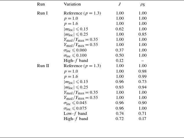
 1/f
 J
 ρS
 f
 f
 f

 B0=1
 B0=6
 V/VA
 k∥
 k⊥
 B0

 B0=6
 V/VA=3
 V/VA=0.7
 1
 2

 Open access

