1 Introduction
The interfacial instability that arises when a heavier fluid is superposed over a lighter fluid is a classic problem in hydrodynamic instability, known as the Rayleigh–Taylor (R–T) instability (Rayleigh Reference Rayleigh1882). A detailed review of the physics of R–T instability may be found in the work of Sharp (Reference Sharp1984). The nonlinear evolution of such an unstable interface is known to exhibit subcritical behaviour that proceeds towards rupture, i.e. the film locally attains zero thickness (Yiantsios & Higgins Reference Yiantsios and Higgins1989). However, in pool boiling experiments, it is often found that a heavier liquid phase is stably supported by an underlying blanket of its less dense vapour (Rajabi & Winterton Reference Rajabi and Winterton1987; Abbassi & Winterton Reference Abbassi and Winterton1989). The presence of such a stable vapour blanket near the heated surface is called the boiling crisis phenomenon and results in unfavourable burnout of heat exchangers (Theofanous et al. Reference Theofanous, Tu, Dinh and Dinh2002). It is the presence of an evaporative phase change that suppresses R–T instability and sustains a vapour blanket adjacent to the heated surface, as shown theoretically by Adham-Khodaparast, Kawaji & Antar (Reference Adham-Khodaparast, Kawaji and Antar1995); Panzarella, Davis & Bankoff (Reference Panzarella, Davis and Bankoff2000) and Kanatani & Oron (Reference Kanatani and Oron2011). The current work aims to investigate the possibility of employing a binary mixture as the working fluid to destabilize the vapour blanket and cause the interface to rupture. This idea is motivated by the fact that a suitable binary mixture, wherein the more volatile component has a lower surface tension with its vapour, can result in solutal Marangoni convection on the liquid–vapour interface that acts to destabilize the system (Uguz & Narayanan Reference Uguz and Narayanan2012; Li & Yoda Reference Li and Yoda2016). To understand why this is so, we first briefly discuss the physics of evaporation in a single-component system, and then proceed to discuss what happens in the case of a binary mixture.
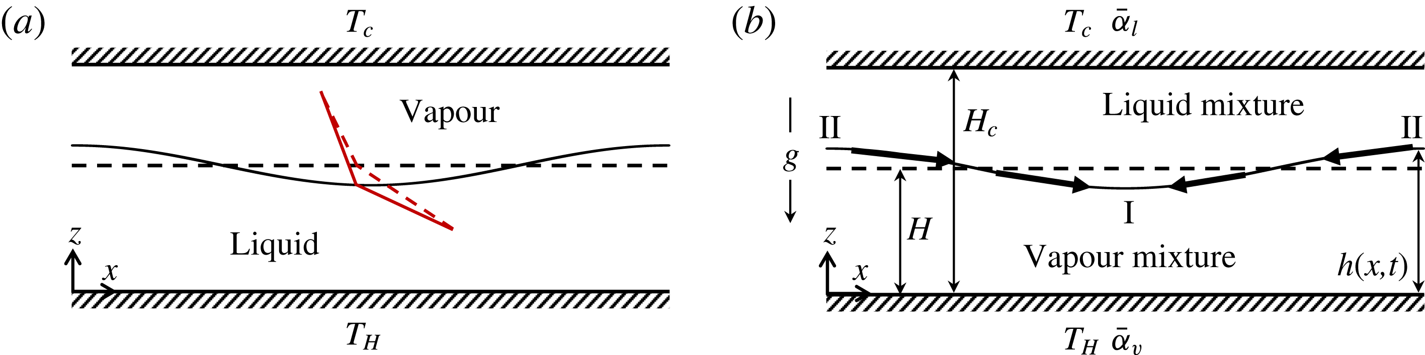
(a) Physical mechanism of evaporation in a single-component system when heated from the liquid side. Dashed lines denote the interface and the local temperature profiles in base state. Solid lines denote the temperature profiles upon perturbation. (b) Schematic of a Rayleigh–Taylor unstable binary mixture, heated from the vapour side. The vapour-side wall is at a hot temperature,
 $T_{H}$
, and high volatile component concentration,
 $\bar{\unicode[STIX]{x1D6FC}}_{v}$
, while the liquid-side wall is at a cold temperature,
 $T_{C}$
, and high volatile component concentration,
 $\bar{\unicode[STIX]{x1D6FC}}_{l}$
.
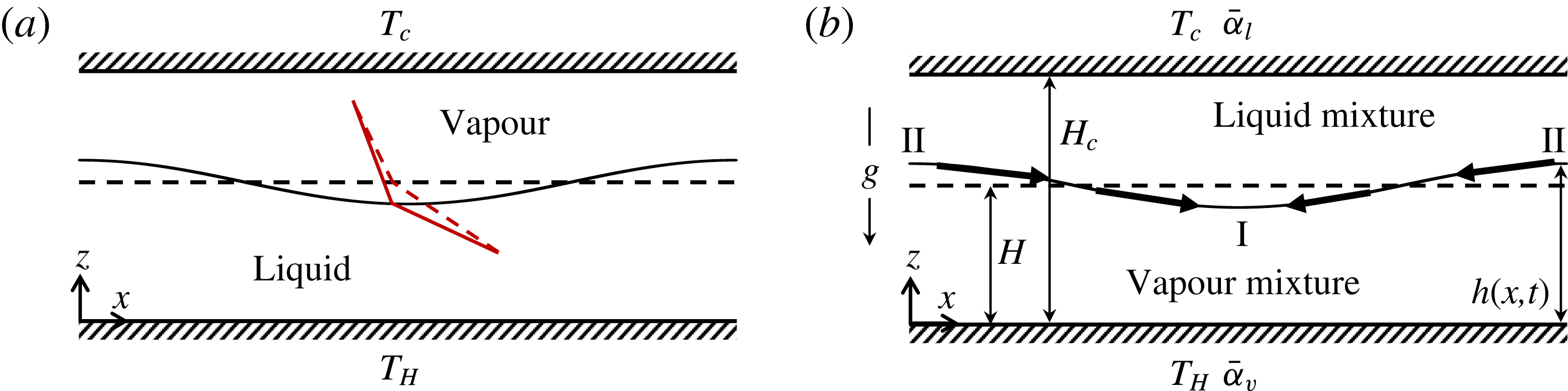
Consider a hermetically sealed liquid–vapour bilayer confined between two flat plates as shown in figure 1(a). The liquid-side wall is maintained at a hot temperature
 $T_{H}$
, while the vapour-side wall is maintained at a cold temperature
 $T_{C}$
. The base state allows a flat interface with no flow, no phase change and a temperature profile characterized purely by thermal conduction. The dashed lines in figure 1(a) depict the base temperature profile at the interface. Now, if we impose a mechanical perturbation on the interface, the trough gets closer to the hot plate and the crest gets closer to the cold plate. At the trough, it then results in a stronger temperature gradient in the liquid and a weaker temperature gradient in the vapour phase (see the solid lines in figure 1
a). Therefore, more heat is transferred from the liquid to the interface and less heat is transferred away to the vapour phase, causing evaporation at the trough. This results in the trough getting deeper, reinforcing the perturbation and causing the interface to be unstable. Such an instability arises even in the absence of gravity or surface tension gradients, and is termed evaporative instability (Miller Reference Miller1973; Ozen & Narayanan Reference Ozen and Narayanan2004), the wavelength being decided by the interfacial tension. It can then be seen that, by inverting the wall temperatures and heating from the vapour side, the interface returns to its base flat state. It is this stabilizing effect of the phase change which sustains a stable vapour blanket below the liquid and manifests as the boiling crisis phenomenon.
Now, let us look at what happens when an evaporating binary mixture is heated from the vapour side in a R–T unstable configuration (liquid on top), as shown in figure 1(b). The vapour-side wall is at a hot temperature,
 $T_{H}$
, and the liquid-side wall is at a cold temperature,
 $T_{C}$
. In the base state, we have no flow with a flat interface and a linear temperature profile in each phase. For any assigned liquid composition, the vapour composition is determined by Raoult’s law and the wall condition could be either one of no-flux or of a constant concentration, as depicted in figure 1(b). When the interface is now perturbed, gravity of course is destabilizing. In addition, as the trough (shown by I) is closer to the hot plate, it acts as the site of evaporation, while condensation takes place at the crest (shown by II). Therefore, liquid moves from region II to I, making the trough deeper and promoting instability for two reasons. First, region I gets more evaporative and therefore richer in the less volatile component. Second, this region which is more concentrated in the less volatile component gets closer to the bottom wall, which again is a source of the less volatile component. This results in a region of higher surface tension at the trough as compared to the crest, thereby promoting the solutal Marangoni flow along the interface. The thermal Marangoni flow, though opposing, is known to be weak in the presence of a phase change (Margerit et al.
Reference Margerit, Colinet, Lebon, Iorio and Legros2003). The objective in this study is to examine the evolution of the interface towards possible rupture in such a case, motivated by its applications to the boiling crisis phenomenon.
The linear stability analyses by Hsieh were the earliest to suggest that R–T instability can be stabilized by evaporation (Hsieh Reference Hsieh1972). Recent works by Kim & Kim (Reference Kim and Kim2016) and Konovalov, Lyubimov & Lyubimova (Reference Konovalov, Lyubimov and Lyubimova2017), based on linear theory, present analytical expressions quantifying the effect of fluid viscosities, layer thickness as well as non-quasiequilibrium effects on the evaporative suppression of R–T instability. The nonlinear dynamics of a R–T unstable interface in the presence of evaporation, using thin-film lubrication models, was investigated by Bestehorn & Merkt (Reference Bestehorn and Merkt2006) and Kanatani & Oron (Reference Kanatani and Oron2011). They showed that the R–T unstable system can be linearly stabilized with strong enough evaporation. When the system is linearly unstable, it may yet nonlinearly saturate to a steady state with a stable vapour blanket, leading to dry-out. To delay dry-out, several experiments have suggested using either binary mixtures (Li & Yoda Reference Li and Yoda2016) or self-rewetting fluids (Savino & Paterna Reference Savino and Paterna2006; Savino, Cecere & Paola Reference Savino, Cecere and Paola2009) as the working fluid. These have reported improved thermal management due to the solutal Marangoni flow generated, with a possibility of delayed vapour film formation and therefore dry-out.
We enquire in the current study if a vapour film, once formed, can rupture due to solutal Marangoni convection. Though linear stability predicts enhanced instability due to solutal Marangoni convection for a binary mixture, to predict whether the instability leads to interface rupture or whether it just leads to a saturated steady state requires a nonlinear computation. Therefore, in the current work, we examine the nonlinear evolution of the interface using a long-wavelength approximation. The results will show that, while an interface under a binary liquid mixture advances more towards a hot vapour wall than an interface under a single-component liquid under the same conditions, it will not rupture. Calculations will also show that the principal reason for this lies in the physics of the fluid flow arising from evaporation. The fluid flow becomes stronger as the interface thins, and ultimately reverses the direction of flow in the liquid phase. The implication of this result is that a vapour film, once formed, cannot easily be destabilized to rupture, at least not by injecting the liquid with a secondary component with the hope of creating Marangoni instability. In what follows, we present the mathematical model and solution methodology in § 2. In § 3 significant results from the model are discussed. A concluding summary of the key results is given in § 4.
2 Mathematical model
A binary Newtonian liquid mixture lying above its own vapour confined between two flat plates is considered (figure 1
b). The nomenclature is denoted in the figure and its caption. Calculations are done using the example of the ethanol–sec-butanol system, with ethanol being the more volatile component. Constant thermophysical properties are assumed, except surface tension (
 $\unicode[STIX]{x1D6FE}$
), which decreases linearly with the concentration of the more volatile component and the lower surface tension. All liquid and vapour variables are denoted with subscripts
 $l$
and
 $v$
. The densities, viscosities, thermal conductivities and species diffusivities are denoted by
 $\unicode[STIX]{x1D70C}_{i}$
,
 $\unicode[STIX]{x1D707}_{i}$
,
 ${\mathcal{K}}_{i}$
and
 $D_{i}$
 $(i=l,v)$
. For a given concentration,
 $\bar{\unicode[STIX]{x1D6FC}}_{i}$
, the liquid and vapour properties are determined from the two components using the mass-averaged mixing rule. The horizontal and vertical components of velocity are denoted by
 $u_{i}$
and
 $w_{i}$
. Both phases are assumed to be thin films and therefore the long-wave approximation
 $(H_{c}\ll \unicode[STIX]{x1D6EC})$
is used, where
 $\unicode[STIX]{x1D6EC}$
is the characteristic horizontal length scale arising from the instability. This separation of length scales helps us to obtain a reduced set of evolution equations for the interface position,
 $h$
, and the phase flow rates,
 $q_{l}$
and
 $q_{v}$
. In thin films, buoyancy convection is insignificant (cf. Zhang Reference Zhang and Savino2006) and is therefore ignored in this study. We follow the weighted-residual integral boundary layer (WRIBL) method as described by Dietze & Ruyer-Quil (Reference Dietze and Ruyer-Quil2013) to obtain the evolution equations.
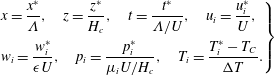
The following scales are used to non-dimensionalize the variables, denoted with an asterisk.
 $$\begin{eqnarray}\displaystyle \left.\begin{array}{@{}l@{}}x={\displaystyle \frac{x^{\ast }}{\unicode[STIX]{x1D6EC}}},\quad z={\displaystyle \frac{z^{\ast }}{H_{c}}},\quad t={\displaystyle \frac{t^{\ast }}{\unicode[STIX]{x1D6EC}/U}},\quad u_{i}={\displaystyle \frac{u_{i}^{\ast }}{U}},\\[11.0pt] w_{i}={\displaystyle \frac{w_{i}^{\ast }}{\unicode[STIX]{x1D716}U}},\quad p_{i}={\displaystyle \frac{p_{i}^{\ast }}{\unicode[STIX]{x1D707}_{i}U/H_{c}}},\quad T_{i}={\displaystyle \frac{T_{i}^{\ast }-T_{C}}{\unicode[STIX]{x0394}T}}.\end{array}\right\} & & \displaystyle\end{eqnarray}$$
Here,
 $\unicode[STIX]{x1D716}$
is a small parameter defined as
 $\unicode[STIX]{x1D716}=H_{c}/\unicode[STIX]{x1D6EC}$
and
 $\unicode[STIX]{x0394}T=T_{H}-T_{C}$
represents the imposed temperature difference across the plates. The characteristic velocity scale,
 $U=\unicode[STIX]{x1D716}^{2}\unicode[STIX]{x1D6FE}/\unicode[STIX]{x1D707}_{l}$
, is obtained by a balance of pressure and capillary forces in the interfacial stress balance.
For very thin films, it is reasonable to assume that the Reynolds numbers are sufficiently small (
 $Re\ll 1$
) so as to neglect all inertial effects. In fact, our computations have shown that while thermal inertia is destabilizing, it cannot override the stabilization due to the evaporation in the long-wave limit. On the other hand, solutal inertia is expected to be stabilizing, and so dropping it gives a conservative prediction of the possibility of rupture. The non-dimensional governing equations obtained using the above scales, after neglecting inertia and other terms of
 $O(\unicode[STIX]{x1D716}^{2})$
and smaller, are
 $$\begin{eqnarray}\displaystyle & \displaystyle {\displaystyle \frac{\unicode[STIX]{x2202}u_{i}}{\unicode[STIX]{x2202}x}}+{\displaystyle \frac{\unicode[STIX]{x2202}w_{i}}{\unicode[STIX]{x2202}z}}=0,\quad -\unicode[STIX]{x1D716}{\displaystyle \frac{\unicode[STIX]{x2202}p_{i}}{\unicode[STIX]{x2202}z}}-\unicode[STIX]{x1D716}\left({\displaystyle \frac{\unicode[STIX]{x1D70C}}{\unicode[STIX]{x1D707}}}\right)^{\unicode[STIX]{x1D6FF}_{iv}}G=0,\quad -\unicode[STIX]{x1D716}{\displaystyle \frac{\unicode[STIX]{x2202}p_{i}}{\unicode[STIX]{x2202}x}}+{\displaystyle \frac{\unicode[STIX]{x2202}^{2}u_{i}}{\unicode[STIX]{x2202}z^{2}}}=0 & \displaystyle\end{eqnarray}$$
 $$\begin{eqnarray}\displaystyle & \displaystyle {\displaystyle \frac{\unicode[STIX]{x2202}^{2}T_{i}}{\unicode[STIX]{x2202}z^{2}}}=0,\quad {\displaystyle \frac{\unicode[STIX]{x2202}^{2}\unicode[STIX]{x1D6FC}_{i}}{\unicode[STIX]{x2202}z^{2}}}=0,\quad \text{where }i=l,v\text{ and }\unicode[STIX]{x1D70C}={\displaystyle \frac{\unicode[STIX]{x1D70C}_{v}}{\unicode[STIX]{x1D70C}_{l}}},\unicode[STIX]{x1D707}={\displaystyle \frac{\unicode[STIX]{x1D707}_{v}}{\unicode[STIX]{x1D707}_{l}}},G={\displaystyle \frac{\unicode[STIX]{x1D70C}_{l}gH_{c}^{2}}{\unicode[STIX]{x1D707}_{l}U}}. & \displaystyle\end{eqnarray}$$
 $\unicode[STIX]{x1D6FF}_{iv}$
is the Kronecker delta function. Equations (2.2a,b
) are the long-wave equations of continuity, momentum, energy and species balance of component A (ethanol). At the walls, no-slip and no-penetration conditions are imposed. In addition, the temperature and concentration satisfy the following boundary conditions:
 $$\begin{eqnarray}\displaystyle & \displaystyle T_{v}=1,\quad \unicode[STIX]{x1D6FC}_{v}=\bar{\unicode[STIX]{x1D6FC}}_{v}\quad \text{at }z=0 & \displaystyle\end{eqnarray}$$
 $$\begin{eqnarray}\displaystyle & \displaystyle T_{l}=0,\quad \unicode[STIX]{x1D6FC}_{l}=\bar{\unicode[STIX]{x1D6FC}}_{l}\quad \text{at }z=1 & \displaystyle\end{eqnarray}$$
 $$\begin{eqnarray}\displaystyle & \displaystyle T_{l}=T_{v},\quad \unicode[STIX]{x1D716}\left(w_{l}-u_{l}{\displaystyle \frac{\unicode[STIX]{x2202}h}{\unicode[STIX]{x2202}x}}-{\displaystyle \frac{\unicode[STIX]{x2202}h}{\unicode[STIX]{x2202}t}}\right)=E_{1}\left({\mathcal{K}}{\displaystyle \frac{\unicode[STIX]{x2202}T_{v}}{\unicode[STIX]{x2202}z}}-{\displaystyle \frac{\unicode[STIX]{x2202}T_{l}}{\unicode[STIX]{x2202}z}}\right)+\unicode[STIX]{x1D70C}E_{2}{\displaystyle \frac{\unicode[STIX]{x2202}\unicode[STIX]{x1D6FC}_{v}}{\unicode[STIX]{x2202}z}}\quad \text{at }z=h\quad & \displaystyle\end{eqnarray}$$
 $$\begin{eqnarray}\displaystyle & \displaystyle \unicode[STIX]{x1D70C}D{\displaystyle \frac{\unicode[STIX]{x2202}\unicode[STIX]{x1D6FC}_{v}}{\unicode[STIX]{x2202}z}}={\displaystyle \frac{\unicode[STIX]{x2202}\unicode[STIX]{x1D6FC}_{l}}{\unicode[STIX]{x2202}z}},\quad p_{v}\unicode[STIX]{x1D714}_{v}=P^{A}\unicode[STIX]{x1D714}_{l}\quad \text{at }z=h. & \displaystyle\end{eqnarray}$$
 ${\mathcal{K}}={\mathcal{K}}_{v}/{\mathcal{K}}_{l}$
,
 $D=D_{v}/D_{l}$
and
 $P^{A}$
denotes the saturation pressure of ethanol (A).
 $E_{1}=({\mathcal{K}}_{l}\unicode[STIX]{x0394}T)/(\unicode[STIX]{x1D70C}_{l}U\bar{{\mathcal{L}}}H_{c})$
is a measure of the latent heat of phase change for the mixture, while
 $E_{2}=({\mathcal{L}}^{A}-{\mathcal{L}}^{B})D_{v}/U\bar{{\mathcal{L}}}H_{c}$
accounts for the enthalpy transferred to the interface due to species diffusion. Here,
 ${\mathcal{L}}^{j}$
denotes the latent heat of the species
 $j$
and
 $\bar{{\mathcal{L}}}={\mathcal{L}}^{A}\bar{\unicode[STIX]{x1D6FC}}_{l}+{\mathcal{L}}^{B}(1-\bar{\unicode[STIX]{x1D6FC}}_{l})$
denotes the mixture latent heat. Also,
 $\unicode[STIX]{x1D714}_{i}$
denotes the ethanol mole fraction and can be related to its mass fraction,
 $\unicode[STIX]{x1D6FC}_{i}$
, using molecular weights. The expression in parenthesis on the left-hand side of (2.3c
) represents the negative of evaporative mass flux (
 $J$
). Using (2.2b
) and (2.3), the temperature and concentration profiles can be obtained solely in terms of the interface position (
 $h$
) and the fluid flow rates (
 $q_{l},q_{v}$
).
We assume thermodynamic equilibrium along the interface, which is valid for low evaporation rates (Huang & Joseph Reference Huang and Joseph1992). The assumption of thermodynamic equilibrium is further justified in our case, wherein we have a hermetically sealed system with no evaporation in the base state. Any phase change happens only due to instability. We use the Clausius–Clapeyron equation in its linear approximation as
 $$\begin{eqnarray}\displaystyle & \displaystyle \unicode[STIX]{x1D707}(P^{j}-P_{ref})=\unicode[STIX]{x1D6F7}^{j}(T_{v}-T_{ref}),\quad \text{where }\unicode[STIX]{x1D6F7}^{j}={\displaystyle \frac{S^{j}\unicode[STIX]{x0394}TH_{c}}{\unicode[STIX]{x1D707}_{l}U}}. & \displaystyle\end{eqnarray}$$
In the above,
 $P^{j}$
is the saturation pressure of the species
 $j$
and
 $S^{j}$
is a dimensional coefficient that appears in the linearized Clausius–Clapeyron equation and has the value
 $S^{A}=4226.2\,\text{Pa}/^{\circ }\text{C}$
and
 $S^{B}=2023.8\,\text{Pa}/^{\circ }\text{C}$
. Also,
 $P_{ref}$
is the saturation pressure at a reference temperature,
 $T_{ref}$
. The non-dimensional parameter,
 $\unicode[STIX]{x1D6F7}^{j}$
, accounts for the relative volatility difference between the two components. It relates the saturation pressure for each component based on the interface temperature, and therefore also determines the interfacial composition through Raoult’s law.
At the interface, the kinematic condition is given by
 $$\begin{eqnarray}\displaystyle & \displaystyle w_{l}-u_{l}{\displaystyle \frac{\unicode[STIX]{x2202}h}{\unicode[STIX]{x2202}x}}-{\displaystyle \frac{\unicode[STIX]{x2202}h}{\unicode[STIX]{x2202}t}}=\unicode[STIX]{x1D70C}\left(w_{v}-u_{v}{\displaystyle \frac{\unicode[STIX]{x2202}h}{\unicode[STIX]{x2202}x}}-{\displaystyle \frac{\unicode[STIX]{x2202}h}{\unicode[STIX]{x2202}t}}\right). & \displaystyle\end{eqnarray}$$
The continuity of velocity at the interface gives
 $u_{l}=u_{v}$
. The tangential and normal stress balances at the interface are
 $$\begin{eqnarray}\displaystyle & \displaystyle \unicode[STIX]{x1D707}{\displaystyle \frac{\unicode[STIX]{x2202}u_{v}}{\unicode[STIX]{x2202}z}}-{\displaystyle \frac{\unicode[STIX]{x2202}u_{l}}{\unicode[STIX]{x2202}z}}=-\unicode[STIX]{x1D716}Ma\left({\displaystyle \frac{\unicode[STIX]{x2202}\unicode[STIX]{x1D6FC}_{l}}{\unicode[STIX]{x2202}x}}+{\displaystyle \frac{\unicode[STIX]{x2202}\unicode[STIX]{x1D6FC}_{l}}{\unicode[STIX]{x2202}z}}h_{x}\right)\quad \text{and}\quad \unicode[STIX]{x1D716}\unicode[STIX]{x1D707}p_{v}-\unicode[STIX]{x1D716}p_{l}=-\unicode[STIX]{x1D716}{\displaystyle \frac{\unicode[STIX]{x2202}^{2}h}{\unicode[STIX]{x2202}x^{2}}},\quad & \displaystyle\end{eqnarray}$$
where
 $Ma=-\unicode[STIX]{x1D6FE}_{\unicode[STIX]{x1D6FC}}/\unicode[STIX]{x1D6FE}$
and
 $\unicode[STIX]{x1D6FE}_{\unicode[STIX]{x1D6FC}}$
denotes the sensitivity of surface tension to ethanol mass fraction. Thermocapillarity is unimportant in the presence of a phase change for a single component (Margerit et al.
Reference Margerit, Colinet, Lebon, Iorio and Legros2003) as well as binary mixtures (Uguz & Narayanan Reference Uguz and Narayanan2012), and therefore has been neglected in the tangential stress balance. It is to be noted that the pressure and curvature terms in the normal stress balance are of the same order. This is due to the implicit assumption of the capillary number (
 $Ca=\unicode[STIX]{x1D707}_{l}U/\unicode[STIX]{x1D6FE}$
) being
 $O(\unicode[STIX]{x1D716}^{2})$
, from the choice of our velocity scale (
 $U=\unicode[STIX]{x1D716}^{2}\unicode[STIX]{x1D6FE}/\unicode[STIX]{x1D707}_{l}$
). This assumption of low capillary number or high surface tension is justified for most practical fluids. Also, the effects of surface tension are known to be usually significant in the long-wave theory of thin films (Oron, Davis & Bankoff Reference Oron, Davis and Bankoff1997), and this order of magnitude assignment to
 $Ca$
retains the effects of interfacial curvature in the long-wave model.
Integrating the vertical component of momentum balance and eliminating pressure, we obtain the usual boundary layer equations (Dietze & Ruyer-Quil Reference Dietze and Ruyer-Quil2013). Next, the boundary layer equations for both phases are multiplied by appropriate weight functions (
 $F_{i}$
) and integrated across each film thickness. We follow the Galerkin method, wherein the weight functions are chosen to be exactly of the same functional form as the locally parabolic velocity profile observed in creeping flow. In the creeping flow limit, this method directly yields the lubrication equations. Whereas, when inertia is retained, the Galerkin method converges faster and turns out to be the most efficient (Ruyer-Quil & Manneville Reference Ruyer-Quil and Manneville2002). The weight functions,
 $F_{i}$
, are therefore defined by
 $$\begin{eqnarray}\displaystyle & \displaystyle {\displaystyle \frac{\unicode[STIX]{x2202}^{2}F_{v}}{\unicode[STIX]{x2202}z^{2}}}=A_{v},\quad {\displaystyle \frac{\unicode[STIX]{x2202}^{2}F_{l}}{\unicode[STIX]{x2202}z^{2}}}=A_{l},\quad F_{v}|_{0}=0,\quad F_{l}|_{1}=0,\quad F_{v}|_{h}=F_{l}|_{h},\quad \left.\unicode[STIX]{x1D707}{\displaystyle \frac{\unicode[STIX]{x2202}F_{v}}{\unicode[STIX]{x2202}z}}\right|_{h}=\left.{\displaystyle \frac{\unicode[STIX]{x2202}F_{l}}{\unicode[STIX]{x2202}z}}\right|_{h}. & \displaystyle \nonumber\\ \displaystyle & & \displaystyle\end{eqnarray}$$
To obtain two equations governing the flow rates of the two phases,
 $q_{v}$
and
 $q_{l}$
, the constants
 $(A_{v},A_{l})$
are chosen to be
 $(1,1)$
and
 $(1,-1)$
for the first and second equation, respectively. The weight functions obtained from these choices of
 $(A_{v},A_{l})$
are denoted by
 $F_{i}^{(+)}$
and
 $F_{i}^{(-)}$
, respectively. The integrals of the weight functions across their respective domains are denoted by
 $I_{i}^{(+)}$
and
 $I_{i}^{(-)}$
. The final set of evolution equations along with the integrated form of the continuity equation are
 $$\begin{eqnarray}\displaystyle & & \displaystyle \displaystyle (\unicode[STIX]{x1D70C}-1){\displaystyle \frac{\unicode[STIX]{x2202}h}{\unicode[STIX]{x2202}t}}=-\left(\unicode[STIX]{x1D70C}{\displaystyle \frac{\unicode[STIX]{x2202}q_{v}}{\unicode[STIX]{x2202}x}}+{\displaystyle \frac{\unicode[STIX]{x2202}q_{l}}{\unicode[STIX]{x2202}x}}\right)\end{eqnarray}$$
 $$\begin{eqnarray}\displaystyle & & \displaystyle \displaystyle \unicode[STIX]{x1D707}q_{v}+q_{l}+\unicode[STIX]{x1D716}MaF_{l}^{(+)}(h){\displaystyle \frac{\text{d}}{\text{d}x}}\unicode[STIX]{x1D6FC}(h)-\unicode[STIX]{x1D716}\unicode[STIX]{x1D707}{\displaystyle \frac{\text{d}}{\text{d}x}}p_{v}(h)(I_{v}^{(+)}+I_{l}^{(+)})-\unicode[STIX]{x1D716}{\displaystyle \frac{\unicode[STIX]{x2202}^{3}h}{\unicode[STIX]{x2202}x^{3}}}I_{l}^{(+)}\nonumber\\ \displaystyle & & \displaystyle \qquad -\,\unicode[STIX]{x1D716}G{\displaystyle \frac{\unicode[STIX]{x2202}h}{\unicode[STIX]{x2202}x}}(\unicode[STIX]{x1D70C}I_{v}^{(+)}+I_{l}^{(+)})=0\end{eqnarray}$$
 $$\begin{eqnarray}\displaystyle & & \displaystyle \displaystyle \unicode[STIX]{x1D707}q_{v}-q_{l}+\unicode[STIX]{x1D716}MaF_{l}^{(-)}(h){\displaystyle \frac{\text{d}}{\text{d}x}}\unicode[STIX]{x1D6FC}(h)-\unicode[STIX]{x1D716}\unicode[STIX]{x1D707}{\displaystyle \frac{\text{d}}{\text{d}x}}p_{v}(h)(I_{v}^{(-)}+I_{l}^{(-)})-\unicode[STIX]{x1D716}{\displaystyle \frac{\unicode[STIX]{x2202}^{3}h}{\unicode[STIX]{x2202}x^{3}}}I_{l}^{(-)}\nonumber\\ \displaystyle & & \displaystyle \qquad -\,\unicode[STIX]{x1D716}G{\displaystyle \frac{\unicode[STIX]{x2202}h}{\unicode[STIX]{x2202}x}}(\unicode[STIX]{x1D70C}I_{v}^{(-)}+I_{l}^{(-)})=0.\end{eqnarray}$$
 $q_{v}$
and
 $q_{l}$
are flow rates associated with the respective phases and are defined as
 $q_{v}=\int _{0}^{h}u_{v}\,\text{d}z$
and
 $q_{l}=\int _{h}^{1}u_{l}\,\text{d}z$
. Equation (2.8) represents our nonlinear model, consistent at first order. We now rescale the system by taking
 $\unicode[STIX]{x1D6EC}\rightarrow H_{c}$
, i.e.
 $\unicode[STIX]{x1D716}=1$
. This implies that in the discussion of our results, physical lengths in both horizontal and transverse directions are scaled with
 $H_{c}$
.
We carry out a linear stability analysis of the evolution equations (2.8) using the method of modal analysis. The base state is assumed to be a static no-flow state with a flat interface. The variables are perturbed around their base state as
 $h=H+h^{\star }\text{e}^{\unicode[STIX]{x1D70E}t+\text{i}kx}$
and
 $q_{i}=q_{i}^{\star }\text{e}^{\unicode[STIX]{x1D70E}t+\text{i}kx}$
, where the starred variables denote the amplitudes of linear perturbations,
 $k$
is the spatial wavenumber and
 $\unicode[STIX]{x1D70E}$
is the corresponding linear growth rate.
For our nonlinear simulations, equations (2.8) are solved with an initial disturbance corresponding to the fastest growing linear mode (
 $k_{m}$
). The initial condition for the time-dependent variables are
 $h(x,0)=H+0.01\cos (k_{m}x)$
and
 $q_{i}(x,0)=0$
. The Fourier spectral collocation technique (Labrosse Reference Labrosse2011) is used to discretize the spatial derivatives in a periodic domain of length
 $2\unicode[STIX]{x03C0}/k_{m}$
. All calculations are carried out with
 $H_{c}=0.5~\text{mm}$
and
 $H=0.3$
. The time integration is performed using the NDSolve subroutine in Mathematica® v.10.3.
3 Results and discussion
The calculations are carried out using the physical properties of ethanol and sec-butanol as listed in Uguz & Narayanan (Reference Uguz and Narayanan2012). Both linear and nonlinear stability analyses are carried out and the observed results are discussed.
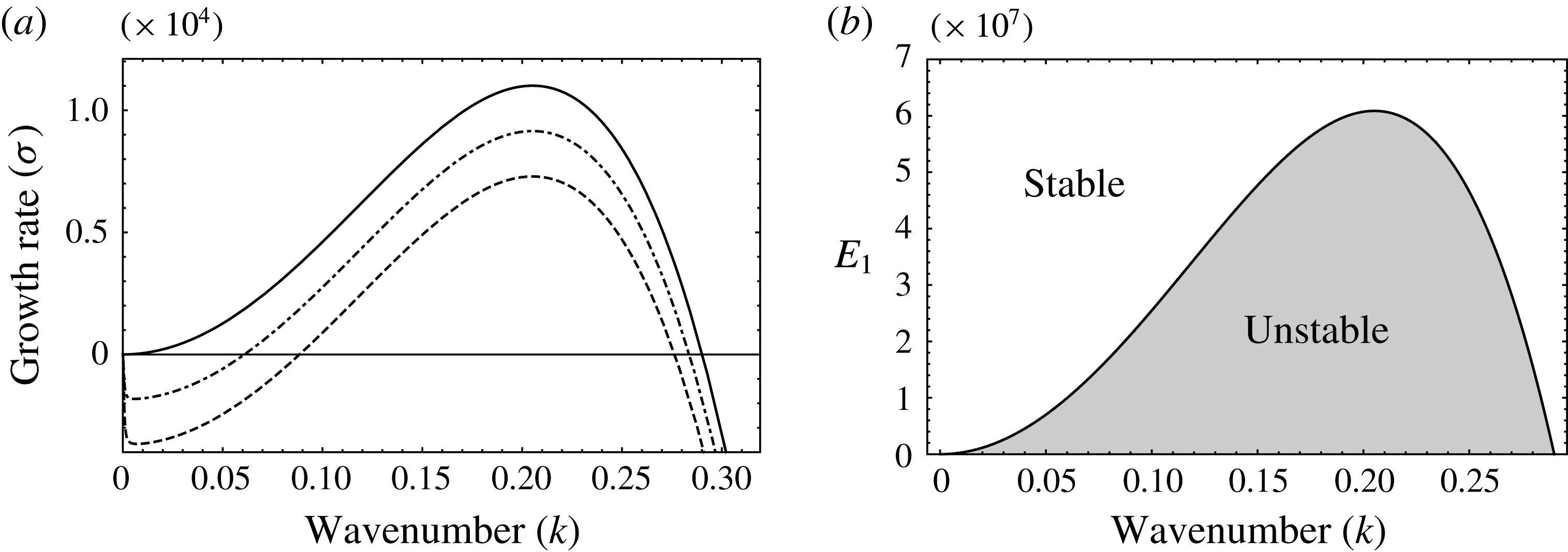
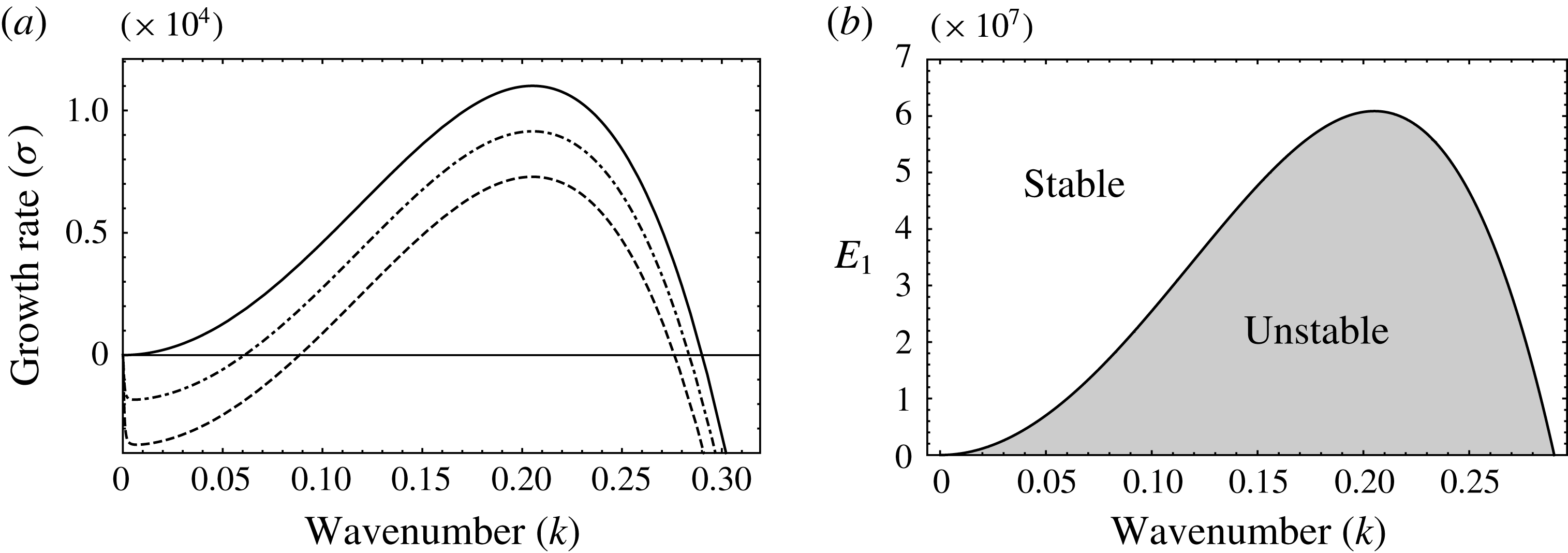
(a) Linear growth rates versus wavenumber for an ethanol bilayer; pure R–T (solid),
 $\unicode[STIX]{x0394}T=5~^{\circ }\text{C}$
(dash-dotted) and
 $\unicode[STIX]{x0394}T=10~^{\circ }\text{C}$
(dashed). (b) Neutral curve corresponding to the division of stable and unstable (shaded) regions.
3.1 Pure-component system
We begin with a discussion on the pure-component evaporation, taking ethanol as an example. An understanding of the physics of this system serves as a basis for comparison with that of the binary mixture of ethanol and sec-butanol discussed later. In figure 2(a), the linear growth rates as a function of wavenumber are plotted for three different cases. The solid curve represents pure R–T instability in the absence of evaporation. The dash-dotted and dashed curves correspond to an imposed
 $\unicode[STIX]{x0394}T=5~^{\circ }\text{C}$
and
 $10~^{\circ }\text{C}$
. It is clear from the panel that the higher the imposed
 $\unicode[STIX]{x0394}T$
, the lower the linear growth rates as well as the range of unstable wavenumbers. This effect of the phase change is depicted clearly in figure 2(b), wherein we have plotted the neutral curve that divides the stable and unstable (shaded) regions in the
 $k-E$
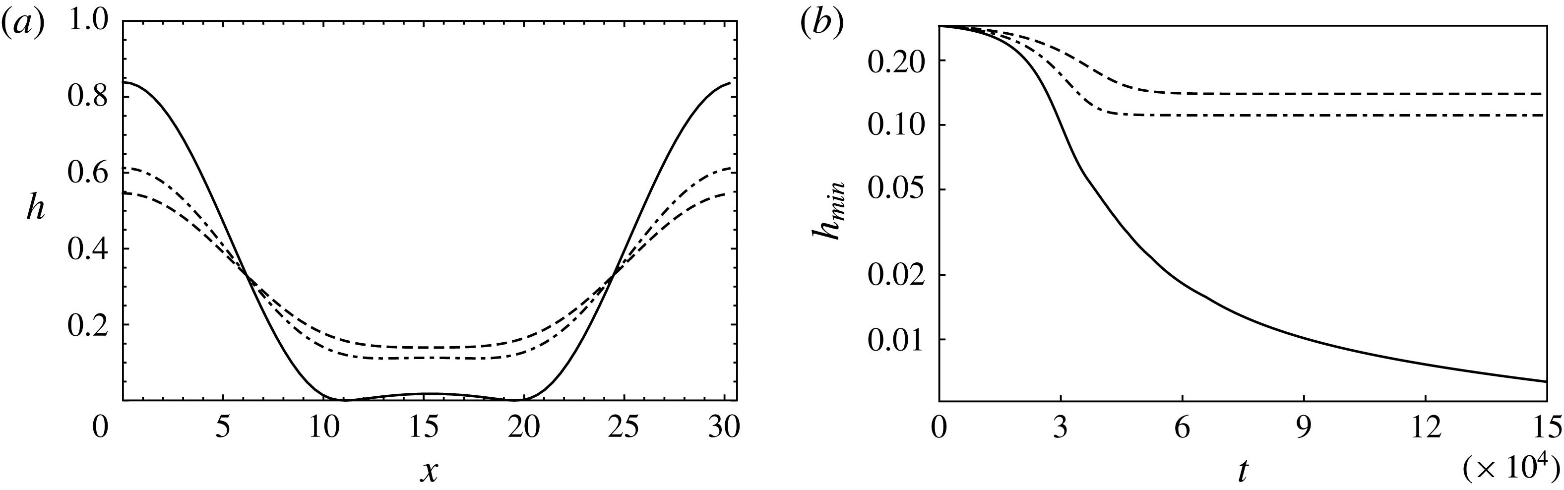
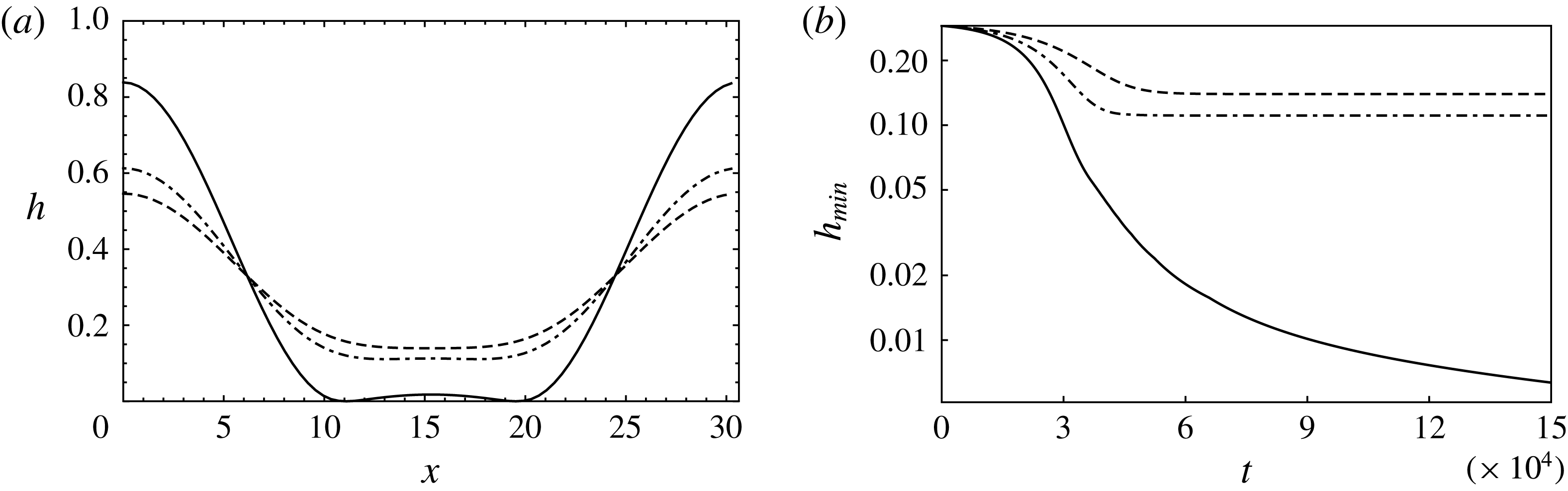
plane. It can be inferred from the figure that sufficiently strong evaporation linearly stabilizes the R–T instability. We next look at the nonlinear evolution of the interface. In figure 3(a), the ‘long-time’ nonlinear configuration attained by the interface corresponding to the fastest growing linear mode (
 $k=0.2$
) is plotted for the three cases discussed earlier. In the pure R–T system (solid), the interface approaches the bottom wall (also see supplementary movie 1 available at https://doi.org/10.1017/jfm.2018.385). This interface profile is in fact a quasi-steady configuration and continues to evolve at very slow rates. This quasi-steady configuration then becomes unstable and exhibits hydrodynamic sliding, rupturing in infinite time (Lister, Rallison & Rees Reference Lister, Rallison and Rees2010). However, in the other two cases of
 $\unicode[STIX]{x0394}T=5~^{\circ }\text{C}$
(dash-dotted) and
 $10~^{\circ }\text{C}$
(dashed), the interface nonlinearly saturates to a steady configuration, as shown in figure 3(a) (also see supplementary movie 2). In figure 3(b), we track the minimum position of the interface (
 $h_{min}$
) as a function of time. It can be seen that although the
 $h_{min}$
corresponding to the pure R–T system (solid) continues towards rupture with time, those corresponding to
 $\unicode[STIX]{x0394}T=5~^{\circ }\text{C}$
(dash-dotted) and
 $10~^{\circ }\text{C}$
(dashed) saturate to a constant value. These results clearly show that evaporation can linearly stabilize R–T instability in a pure-component system. Also, when linearly unstable, evaporation results in a nonlinear saturation of the interface away from the wall, preventing rupture. Next, we look at the binary mixture of ethanol and sec-butanol and investigate the possibility of rupture, due to solutal Marangoni convection.
(a) The ‘long-time’ nonlinear configuration attained by the interface in an ethanol bilayer for pure R–T (solid),
 $\unicode[STIX]{x0394}T=5~^{\circ }\text{C}$
(dash-dotted) and
 $\unicode[STIX]{x0394}T=10~^{\circ }\text{C}$
(dashed). (b) Corresponding temporal evolution of the minimum position of the interface.
3.2 Binary mixture
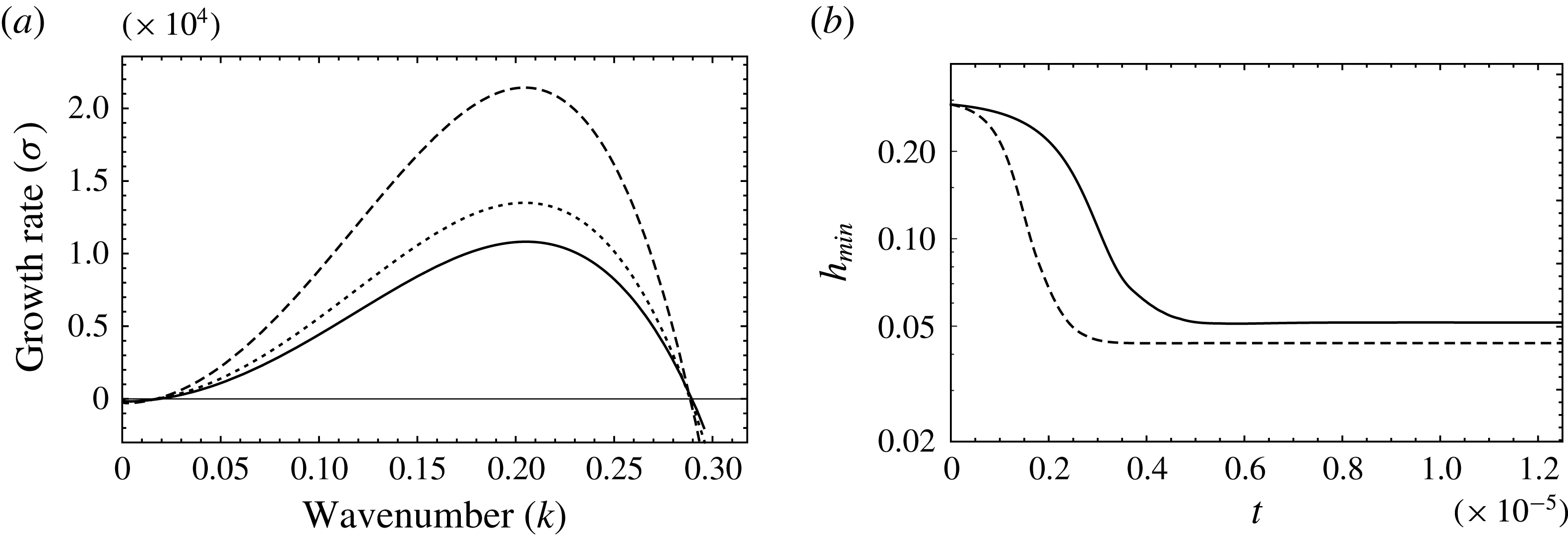
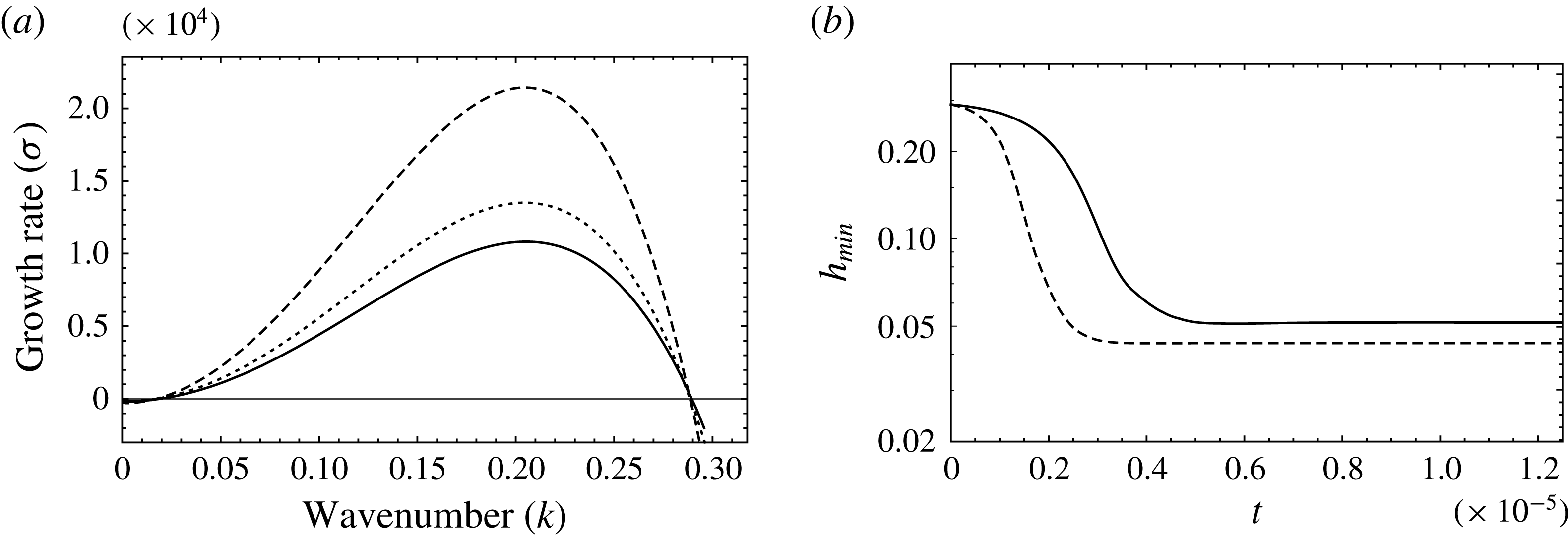
In figure 4(a), the linear growth rates as a function of wavenumber are plotted for different concentrations of the binary mixture. The solid line represents pure ethanol, the dotted line represents a 80–20 mixture and the dashed line represents a 50–50 mixture. It can be seen that the binary mixture always exhibits higher linear growth rates and therefore enhanced instability as compared to the pure-component system. This enhanced instability is due to the solutal Marangoni convection associated with the binary mixture. The relative volatility between the two components, characterized primarily by the difference in the values of
 $\unicode[STIX]{x1D6F7}^{j}$
of the two components, on evaporation, generates a concentration gradient that drives the fluid to destabilize the system as discussed in § 1. Typically, the greatest instability is observed for concentration values close to
 $\bar{\unicode[STIX]{x1D6FC}_{l}}=0.5$
. This is because destabilization offered by phase-change-induced solutal Marangoni flow is its strongest when both species are present in significant amounts, as compared to pure-component systems, wherein no solutal Marangoni flow is possible. We restrict the rest of our analysis to a binary mixture corresponding to the concentration,
 $\unicode[STIX]{x1D6FC}_{l}=0.5$
. Now that the binary mixture results in higher linear growth rates, we proceed to study its nonlinear evolution. In figure 4(b), we plot the minimum position of the interface with time for a pure and binary mixture corresponding to an imposed
 $\unicode[STIX]{x0394}T=0.5~^{\circ }\text{C}$
. The solid line denotes pure ethanol and the dashed line denotes the 50–50 binary mixture. It can be seen that
 $h_{min}$
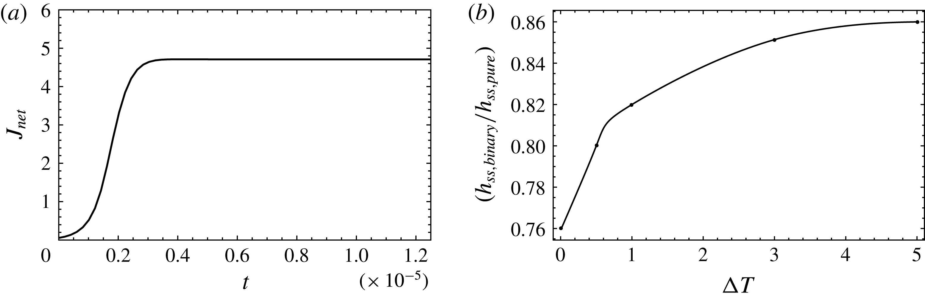
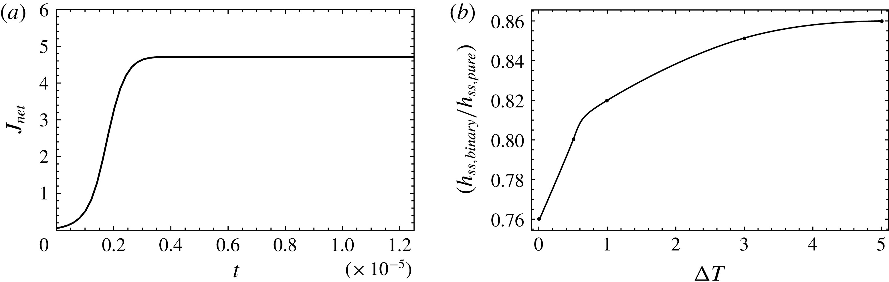
for the binary mixture evolves at a faster rate, consistent with the enhanced instability predicted by linear theory. Although the rate of interface evolution is accentuated, it is interesting to note that the interface exhibits nonlinear saturation, even in the case of the binary mixture, albeit closer to the wall on the vapour side. To see why this is so, we have plotted the scaled net mass flux due to the phase change,
 $J_{net}$
, as a function of time for the binary system in figure 5(a). Here,
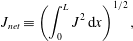 $$\begin{eqnarray}\displaystyle & \displaystyle J_{net}\equiv \left(\int _{0}^{L}J^{2}\,\text{d}x\right)^{1/2}, & \displaystyle\end{eqnarray}$$
where
 $J$
is the local mass flux across the interface and has been scaled with
 $E_{1}$
. It can be seen from figure 5(a) that the net mass flux due to the phase change exhibits a strong nonlinear increase with time as the interface approaches the wall on the vapour side. Therefore the stabilizing effect of the phase change becomes stronger as the interface approaches rupture. Thereafter, when the interface reaches its steady configuration,
 $J_{net}$
also assumes a constant value.
(a) Linear growth rates versus wavenumber for a binary mixture of ethanol sec-butanol for
 $\unicode[STIX]{x0394}T=0.5~^{\circ }\text{C}$
; solid – pure ethanol, dotted – 80–20 mixture (
 $\bar{\unicode[STIX]{x1D6FC}_{l}}=0.80$
), dashed – 50–50 mixture (
 $\bar{\unicode[STIX]{x1D6FC}_{l}}=0.5$
). (b) Temporal evolution of the minimum position of the interface; solid – pure ethanol for
 $\unicode[STIX]{x0394}T=0.5~^{\circ }\text{C}$
, dashed – 50–50 mixture (
 $\bar{\unicode[STIX]{x1D6FC}_{l}}=0.5$
).
(a) Time evolution of the net evaporative mass flux (
 $J_{net}$
) for the binary system,
 $\unicode[STIX]{x0394}T=0.5~^{\circ }\text{C}$
. (b) The ratio of the steady state minimum position of the interface for the binary mixture to that of the pure ethanol bilayer.
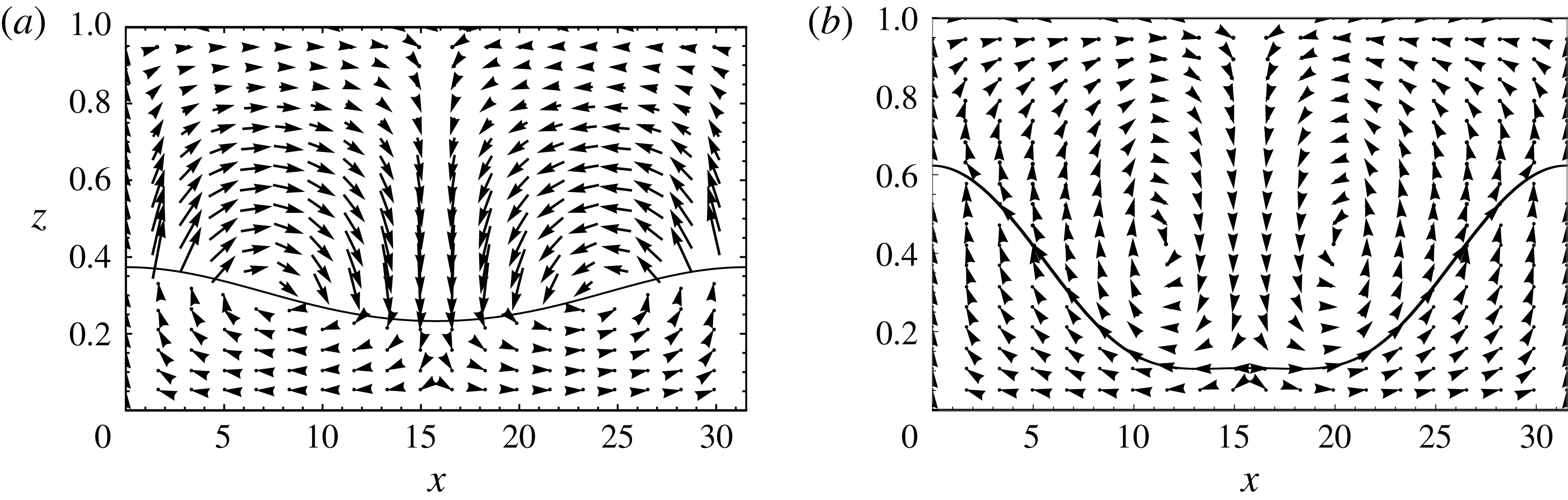
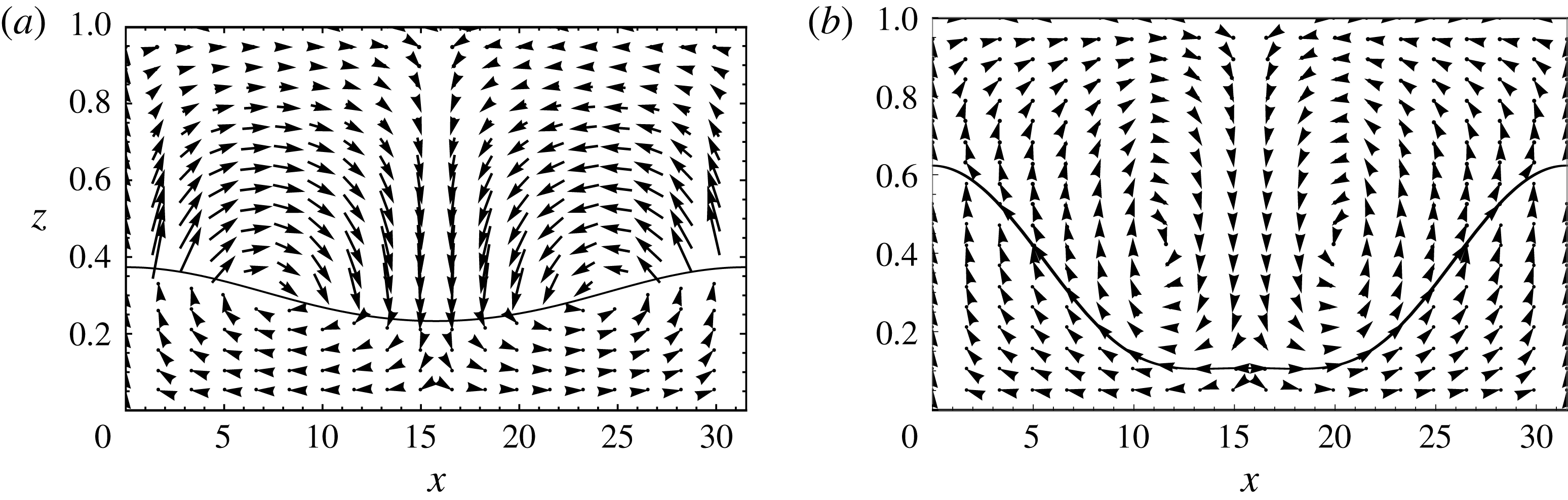
In figure 6, the typical velocity profiles in each phase are plotted for an initial transient time (figure 6
a) as well as for the final steady state (figure 6
b). From figure 6(a), it is clear that, during the initial transients, the velocity in the liquid is driven by the destabilizing solutal Marangoni convection (crest to trough), consistent with the linear theory. However at steady state, figure 6(b) shows that the direction of flow is reversed and driven by the phase change (trough to crest). This implies that in the vicinity of the heated wall, evaporation gets increasingly stronger and creates a flow-reversal in the liquid phase that overcomes the destabilizing Marangoni flow (see supplementary movie 3). The decrease in the solutal Marangoni effect with an increasing net mass flux due to evaporation is also clear from figure 5(b). Here, we have plotted the ratio of the minimum position of the interface (
 $h_{min}$
) attained at steady state by the binary mixture to that of the pure-component system as a function of the imposed
 $\unicode[STIX]{x0394}T$
. When this ratio approaches a value of 1, both the pure-component and the binary system saturate to the same nonlinear steady configuration. As can be seen from the figure, this ratio approaches 1 as the imposed
 $\unicode[STIX]{x0394}T$
increases. Therefore, the difference between a binary and pure-component system decreases with an increase in the imposed
 $\unicode[STIX]{x0394}T$
, or correspondingly when the net evaporative mass flux is high. A low
 $\unicode[STIX]{x0394}T$
is therefore needed for the solutal Marangoni effect to affect the nonlinear dynamics of the system, and thereby its final steady configuration. The condition for a binary mixture to exhibit rupture, while the pure component exhibits nonlinear saturation, thus happens only at impractically low values of
 $\unicode[STIX]{x0394}T$
.
The interface position and velocity fields in each phase for a binary mixture: (a) during the initial transient stage and (b) in the final steady configuration. Only vector heads are plotted to indicate the direction of flow,
 $\unicode[STIX]{x0394}T=5~^{\circ }\text{C}$
. Observe the flow-reversal in the liquid near the interface as it approaches the heated bottom wall. Also see supplementary movie 3.
4 Conclusions
A binary mixture with the more volatile component having a lower surface tension may become unstable due to the solutal Marangoni flow. R–T instability in such a binary mixture undergoing a phase change exhibits higher linear growth rates as compared to the pure-component system. The Marangoni destabilization so obtained is not sufficient to cause rupture for practical operating conditions. The stabilizing effect of phase change creates a flow-reversal on the liquid side that overcomes the destabilizing Marangoni flow. The consequence of this study is the observation that a vapour film once formed under the phase change does not collapse despite the destabilization offered by concentration gradients or gravity.
Acknowledgements
We are grateful to NSF via NSF-0968313 and NASA via NNX17AL27G for financial support. R.N. acknowledges support from a Fellowship awarded by the Institute of Advanced Study – Durham University, UK.
Supplementary movies
Supplementary movies are available at https://doi.org/10.1017/jfm.2018.385.