


Paid television advertising commands the largest portion of the communications budget in campaigns for the most important elective offices and represents an important source of voter information about candidates. Despite increased use of Internet communications and renewed attention to voter mobilization fieldwork, big campaigns are still essentially paid media battles that aim to persuade voters. Our study addresses two unresolved questions regarding the persuasive influence of mass media campaigns: What is the effect of television and radio campaign advertising on voter preferences? How long do the effects last? After addressing these issues we use our empirical results to consider an important further question: What do our results suggest about how voters process political information?
We analyze the findings of a randomized field experiment measuring the size and duration of campaign effects caused by a $2 million television and radio buy. There are two main results. First, across a range of model specifications, television campaign advertisements have a large and statistically significant effect on voter preferences. Second, and perhaps most surprising, the effects of the advertisements dissipate rapidly. Nearly all previous research on advertising effects has ignored the issue of decay and implicitly assumes that decay, if it occurs, takes place over weeks or months. We find that just a week or two later, the advertisement's effects have all but disappeared.
The arresting finding of sizable effects and rapid decay has important implications for our understanding of campaign strategy and the effect of campaign spending on election outcomes. The results also have implications for alternative models of voter learning. As we explain at greater length in the discussion section of our paper, a large initial response followed by a quick return to pretreatment opinions does not fit well with models of on-line processing. In these models, existing opinions are adjusted when new information is received and then the resulting new opinions are maintained, even if the information that caused the change is forgotten. We find that campaign advertising causes a large initial boost in support for the sponsor, but this effect diminishes rapidly over time. This up and then down pattern is far more consistent with opinion change due to priming effects, where the advertising temporarily alters the mix of considerations that are salient for the respondent at the moment the respondent is asked to state an opinion.
Despite the substantial attention that the media's influence has received, no real-world experiments have measured the size and duration of effects of a candidate's media campaign. This is an important gap, as the use of random assignment in a field context addresses a number of potential methodological vulnerabilities in earlier work. Random assignment enables laboratory studies to detect causal effects, but the external validity of these measurements remains uncertain. Observational studies, despite recent advances in measurement and design, cannot identify the causal effects of advertising without invoking strong assumptions about unobserved factors that might be correlated with advertising and vote choice. To date, field experiments involving mass media have focused exclusively on nonpartisan messages, and no field experiment has come close to deploying television communications on the scale and intensity of an actual statewide campaign.Footnote 1
Our research attempts to fill this gap by evaluating a $2 million television and radio campaign. This three-week campaign encompassed 18 television media markets (designated market areas, hereafter “DMAs”) and more than 80 AM and FM radio stations. At its peak, the experimental campaign deployed up to 1,000 gross ratings points (GRPsFootnote 2) of advertising per week into selected DMAs, which is comparable to what battleground states experience during the fall of a presidential election year (Johnston, Hagen, and Jamieson Reference Johnston, Hagen and Jamieson2004). We track outcomes using a large daily tracking poll, which gathered approximately 1,000 interviews per day (for analyses of media effects using large tracking polls, see Hill et al. Reference Hill, Lo, Vavreck and Zaller2010; Huber and Arceneaux Reference Huber and Arceneaux2007; Johnston, Hagen, and Jamieson Reference Johnston, Hagen and Jamieson2004).
The remainder of this essay is structured as follows. We describe the prior literature on the effects of media campaigns. No previous field experiments have measured the effects of a partisan media campaign, and very little work of any sort has estimated the decay rate of campaign advertising. We then describe the gubernatorial race that provides the setting for our experiment and the television and radio ads that were the focus of our experimental evaluation. Next we describe the design of the experiment and the survey that we used to assess outcomes. We then present an array of cross-sectional time-series models that parameterize media effects in different ways. We conclude by discussing the implications of our findings for competing hypotheses about how voters process campaign information.
PREVIOUS LITERATURE
Our research is the first field experiment assessing a large-scale partisan campaign and introduces a new approach to the decades-old scholarly effort to understand the effects of media campaigns on attitudes and behavior. The persuasiveness of mass media communications has been hotly debated since the dawn of modern social science during the 1930s. Although most political observers accorded enormous weight to radio, newsreels, and, later, television communication, early students of political propaganda tended to downplay these effects. The survey findings of Lazarsfeld, Berelson, and Gaudet (Reference Lazarsfeld, Berelson and Gaudet1944), coupled with the controlled experiments of Hovland, Lumsdaine, and Sheffield (Reference Hovland, Lumsdaine and Sheffield1949), called into question the persuasiveness of political communication and ushered in the “minimal effects” thesis (Klapper Reference Klapper1960) that would hold sway among academics until the 1980s. In contrast, the overwhelming majority of more recent studies reach a different judgment, finding that media campaigns can have substantial effects. Using a variety of research designs, scholars have concluded that mass media campaigns can have important effects on voter attitudes and behavior.
One common research strategy employs survey data and correlates self-reported media exposure, measured by reported media usage or reported campaign advertising exposure, with voter opinions (e.g., Baum Reference Baum2002). These studies tend to find very strong media effects, but the results are vulnerable to selection bias (respondent viewing patterns may be correlated with existing political views) and measurement bias (measurement error in self-reports of exposure may be correlated with political views).Footnote 3 Many recent studies improve on self-reported exposure measures by obtaining measurements of the advertising actually aired in the respondent's media market (Freedman, Franz, and Goldstein Reference Freedman, Franz and Goldstein2004; Freedman and Goldstein Reference Freedman and Goldstein1999; Huber and Arceneaux Reference Huber and Arceneaux2007; Johnston, Hagen, and Jamieson Reference Johnston, Hagen and Jamieson2004). However, because advertising levels are chosen by the campaigns, the level of advertising exposure that a survey respondent's area receives may be correlated with other differences across places, including the level of targeted campaign activity (such as mailings, visits, phone calls), that are hard to measure accurately.
Several recent studies of media effects give careful attention to causal identification and aim to uncover and analyze “natural experiments” (Ashworth and Clinton Reference Ashworth and Clinton2006; DellaVigna and Kaplan Reference DellaVigna and Kaplan2007; Huber and Arcenaux Reference Huber and Arceneaux2007; Krasno and Green Reference Krasno and Green2008). The study most similar in spirit to our work is DellaVigna and Kaplan (Reference DellaVigna and Kaplan2007), which uses the staggered national rollout of the Fox News channel to estimate the effect of Fox News on voting in the 2000 presidential election. Comparing the change in Republican vote share between 1996 and 2000 in places that began receiving Fox News between 1996 and 2000 with those places that did not yet receive Fox News, the authors find that receiving Fox News boosted the Republican vote share by approximately 0.5 percentage points. The Della Vigna and Kaplan estimation strategy rests on the key assumption that, after conditioning on the control variables, regions that receive Fox News during the 1996 to 2000 period are politically similar to regions where Fox News was introduced after the 2000 election. Like DellaVigna and Kaplan, we employ a staggered introduction of the media “treatment,” but we use random assignment to determine the timing of the ads. By design, the timing of our treatment is statistically independent of unmeasured differences in political opinions.
Laboratory studies of campaign effects overcome many of the diverse threats to internal validity present in observational studies. Experiments have suggested that television news shapes what issues the public considers important (Iyengar, Peters, and Kinder Reference Iyengar, Peters and Kinder1982), that the tone of televised advertising influences voter cynicism (Ansolabehere and Iyengar Reference Ansolabehere and Iyengar1995), and that the content of news stories shapes public opinion toward race-related policies (Gilliam and Iyengar Reference Gilliam and Iyengar2000). Campaign advertisements are found to significantly increase voters’ support for the sponsoring candidates (Ansolabehere and Iyengar Reference Ansolabehere and Iyengar1995, 186; Brader Reference Brader2005, 395; Kaid Reference Kaid1997, 1088; Valentino, Hutchings, and Williams Reference Valentino, Hutchings and Williams2004, 349). These results are highly suggestive. However, although laboratory studies often go to great lengths to simulate a naturalistic viewing environment, it is unclear whether the laboratory findings parallel the direction and magnitude of voter responses and campaign effects in real world settings. Rarely do laboratory studies gauge the duration of media effects (Gaines, Kuklinski, and Quirk Reference Gaines, Kuklinski and Quirk2007). It is unclear whether the effects produced through laboratory interventions are as long-lasting as those produced by campaigns in typical real world settings.
Surprisingly little research of any kind addresses the decay of political advertising effects. Although some work has shown decay in recall (Lodge, Steenbergen, and Brau Reference Lodge, Steenbergen and Brau1995), decay is not estimated in leading studies of the impact of advertising on voter attitudes and behavior (e.g., Hillygus and Shields Reference Hillygus and Shields2008; Huber and Arceneaux Reference Huber and Arceneaux2007; Johnston et al. Reference Johnston, Blais, Brady and Crete1992; Johnston, Hagen, and Jamieson Reference Johnston, Hagen and Jamieson2004; Shaw Reference Shaw1999), which implicitly assume that advertising effects endure for several weeks or months. Empirical studies of campaign spending effects, starting with Jacobson (Reference Jacobson1978), correlate election results with total incumbent and challenger spending over the course of the campaign. Studies linking recalled exposure to survey responses do not make fine distinctions regarding how recent the exposure is. The prevailing inattention to the duration of effects is reflected in the standard ANES questions regarding campaign exposure. Respondents are asked questions such as “Do you recall seeing any ads for political candidates on television this fall?” This item does not account for the possibility that exposure last week is materially different from exposure the week before last, let alone exposure a month or two earlier.
Decay is generally neglected in political science research, but there is a small literature on decay of product advertising effects, which concludes that there is rapid decay in recall of the advertisement (Burke and Srull Reference Burke and Srull1988; Vakratsas and Ambler Reference Vakratsas and Ambler1999; Zielske and Henry Reference Zielske and Henry1980), attitudes toward the product (Haugtvedt et al. Reference Haugtvedt, Schumann, Schneier and Warren1994), and purchase intention (Havlena and Graham Reference Havlena and Graham2004). The speed of decay can sometimes be determined from the data presented in these reports. For example, Zielske and Henry (Reference Zielske and Henry1980) use survey data on recall of the advertisement and data on television advertising buys to estimate that recall falls by about 10% each week. Qualitatively similar findings are reported in the laboratory experiments of Haugtvedt et al. (Reference Haugtvedt, Schumann, Schneier and Warren1994), although decay rates vary across laboratory experimental conditions and are only measured a single time (1 week) after initial advertising exposure.
The only recent work that focuses on the decay rate of political advertising is a pair of observational studies by Hill et al. (Reference Hill, Lo, Vavreck and Zaller2010). Hill et al. use survey data and data on advertising buys to estimate a dynamic model of decay rates across a variety of campaigns.Footnote 4 This study, which hinges on the assumption that the timing and extent of advertising volume are exogenous, indicates that the impact of advertising in House, Governor, and Senate elections in 2006 has a half-life of between two and three days, whereas presidential advertising in the 2 months prior to the 2000 election has a half-life of about 1 week. They also find some evidence that decay rates vary with political awareness; advertising effects decay more rapidly for the least politically aware. Our experimental results, which were obtained independently and based on an experiment performed prior to the November 2006 election, complement the Hill et al. research by providing a firm methodological basis for the finding that some campaign advertising may have a much shorter half-life than previously expected.
DESCRIPTION OF THE EXPERIMENTAL SETTING
Our analysis focuses on the 2006 reelection campaign of Texas governor Rick Perry. Aside from its receptiveness to experimental evaluation, the Perry campaign started off much like other big-state reelection campaigns. Perry became the Republican governor of Texas in 2000, succeeding George W. Bush when the latter resigned after winning the presidency. Perry had from 1985 to 1991 served two terms as the Commissioner of Agriculture and in the Texas House of Representatives. With deep Texas roots in a rural part of West Texas, Perry had solid conservative credentials that put him squarely in the middle of the Texas mainstream. In 2002, Perry was reelected governor, winning decisively over a well-financed Democratic opponent by a 58 to 40% margin.
The 2006 race presented a more difficult reelection test. Early signs indicated that the public had a far dimmer view of President Bush's performance heading into the 2006 race than they had heading into the 2002 contest. Perry also faced some internal strife within his own legislative majority, after action on an important education finance package stalled during the 2005 legislative session. During the first half of 2005, Perry's popularity ratings declined, and it appeared that he might face a stiff challenge in the GOP primary from U.S. Senator Kay Bailey Hutchinson. But in July 2005, Hutchinson decided not to challenge Perry, and in September Hurricane Katrina put the Governor's leadership on display through a surge in media coverage. His approval rating rebounded to its highest level in three years, just above 50%. Even so, a threatened primary challenge from state comptroller Carole Keeton Strayhorn kept the Perry camp on edge though the end of 2005. Although a less formidable opponent than Hutchinson, Strayhorn was a credible challenger, with her own distinguished record of public service. Strayhorn was the first female mayor of Austin and the only mayor elected for three successive terms. She was also the first woman elected Texas Railroad Commissioner—a position that has often been considered a stepping stone to the governorship.
The late filing deadline meant that final announcement of a Strayhorn primary challenge could wait until the beginning of January, which, with early voting in Texas, meant a potentially short and intense battle for the nomination in early March. In the fall of 2005, Strayhorn aired a series of radio ads that were critical of the governor. In December, she purchased several hundred thousand dollars worth of television time to air in January, presumably to kick off a nomination challenge; the Perry campaign countered by buying three weeks of advertising that form the basis of this experiment. However, on the day of the deadline, January 2, she announced her intention to run as an Independent, which meant that January 2 marked an end to the primary contest and the beginning of the general election campaign.
As noted below, the media campaign launched in January by Texans for Rick Perry was conceived in December, before it was known that Strayhorn would not be running in the primary. The Strayhorn campaign deployed a television and radio ad during the first three weeks of January in selected media markets, but did not advertise during the rest of the primary season. The other candidates, for their part, deployed no media advertising in January. During the early months of 2006, none of the candidates fielded more than a small ground campaign. Campaign communications were almost exclusively deployed through television and radio.
To be sure, the circumstances of this experiment are unusual: the start of a yearlong campaign in which a GOP incumbent governor squared off against two independent candidates and an as yet unnominated Democrat. At the same time, the manner in which ads were deployed closely approximates what Zaller (Reference Zaller, Mutz, Brody and Sniderman1996) describes as the ideal conditions for detecting media effects: well-measured, abrupt shifts in the quantity of advertising; a vacuum or profusion of opposing ads; a single ad that is deployed through the three-week experimental period, with no ads preceding or following it; and continuous tracking of opinion before, during, and after the flight of advertising. Although this experiment cannot tell us how media effects might play out under different conditions, it does speak with special clarity to the question of whether paid advertising is capable of producing noticeable shifts in voter support.
THE EXPERIMENTAL CAMPAIGN ADS
Texans for Rick Perry kicked off its campaign with an advertising message that highlighted the governor's accomplishments and charisma. In an attempt to appeal to a broad spectrum of Texas voters, the television ad sought to link positive images of the photogenic governor with voters’ pride in the state of Texas. The scenes sweep from Texas landscapes to a schoolroom to a doctor's office, with Governor Perry's voiceover:
I've never been more proud to call myself a Texan. In Texas we've set the national standard for economic development. We gained 300,000 new jobs. Lawsuit reform is bringing better healthcare to millions. We've invested ten billion new dollars in our public schools while improving standards of accountability for student performance. Our people are compassionate. Our vision, bold. Our values, strong. The best is yet to come. I'm proud of Texas. How ’bout you?
Two aspects of this ad are noteworthy. First, it appeals only indirectly to voter ideology, focusing instead on their retrospective performance evaluations and what Stokes (Reference Stokes1963) dubbed “valence” issues. Oblique ideological reference is made to “lawsuit reform,” “improved standards of accountability for student performance,” and strong values, but these conservative themes are balanced by willingness to spend more on education. The emphasis throughout is on accomplishments and the pride that Texans should take in their state and the governor's stewardship. The visuals shift from one iconic Texas image to another, interspersed with images of a handsome suit-clad governor milling with workers and children or poised in front of the State Capitol.
Second, the ad makes no mention of opponents or their platforms or attributes. The script does not even conjure up implicit critiques of the challengers by referring to the governor's “proven leadership” or other personal traits. This tactic reflects the strategic setting at the time during which the ads aired. Carole Keeton Strayhorn had limited name recognition (at least with that particular name—she was known to some Texans by a last name that she dropped after her remarriage), as did the two Democratic contenders for their party's nomination. By “going positive,” the Perry campaign sought to deny its opponents the salience that comes with back-and-forth in both the paid media and accompanying news coverage. Although no single ad can ever be said to be representative of the population of ads aired by well-funded media campaigns, it should be noted that the Wisconsin Advertising Project's content analysis of TV ads by U.S. Senate candidates in 2004 found that positive promotion ads, such as Perry's, comprised 46% of all ads aired in competitive races and 69% of all ads aired in uncompetitive races (Franz et al. Reference Franz, Freedman, Goldstein and Ridout2008).
The radio ad followed a similar format but with more specific references to accomplishments. The text of the ad can be found in supplementary online Appendix A (available at http://www.journals.cambridge.org/psr2011005). The overall theme is that voters have ample reason to be proud of Texas given the many ways in which the state has excelled under Governor Perry's leadership. Although no mention is made of a political campaign—no requests for voters’ support, for example—the television and radio ads implicitly anticipate criticisms by other candidates.Footnote 5
EXPERIMENTAL DESIGN
This section explains how the random assignment was performed and the implications for the statistical analysis that follows. For the broadcast television and radio experiments, the cross-sectional unit of observation is the DMA, or designated media market. Texas comprises 20 such markets of varying geographic and population size. These broadcast media markets also define the boundaries of cable TV systems, which are obligated to carry advertising purchased on broadcast stations. Approximately two-thirds of all households at this time subscribed to cable television.Footnote 6
Of these 20 media markets, the campaign was willing to allow experiments in 18, regarding the other two (Houston and Dallas–Fort Worth) as too politically important to leave to chance. In light of the heterogeneity of the DMAs, we matched them as closely as possible based on demographic and socioeconomic attributes and then randomly assigned members of each stratum into an ordering that indicated the start date of the broadcast television campaign. See online Appendix C for a list of these matches. Within each weekly rollout bracket, we randomly assigned the quantity of weekly GRPs to be purchased: 250, 500, or 1,000. The rollout dates were then given to the campaign's television media buyer, who arranged to purchase the quantity of broadcast TV ads that we specified for each DMA each week.Footnote 7 Given the small number of DMAs, the power of the experiment derives from the over-time changes in advertising within DMAs, and the analysis presented below focuses on the within-subjects design.
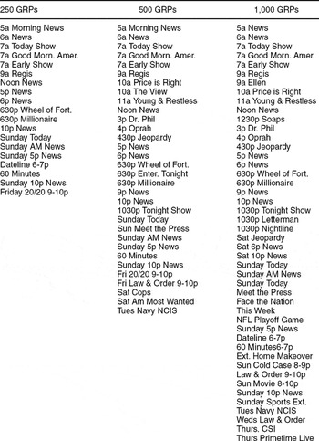
The experiment did not randomize the stations and programs on which the ads were placed. Broadcast TV ads were purchased in a variety of stations based on the campaign consultants’ strategic judgment. Table 1 illustrates the sort of advertising purchases that were made in three DMAs that varied in terms of the quantity of advertising to which they were randomly assigned. A DMA assigned 250 GRPs aired most of the Perry ads on morning shows and news programs. A DMA assigned 500 GRPs bolstered the morning and news programming with additional entertainment programming. At 1,000 GRPs, the quantity of entertainment programs increased further, and the range of shows extended into late night entertainment and news programs. Future work may attempt to estimate the distinct effects of a fixed supply of GRPs spread over a varying number of shows or the effects of greater GRP weight within a given set of shows.
Illustration of Programming on Which Broadcast TV Ads Aired in Three DMAs, by Gross Ratings Points

Once the broadcast TV rollout brackets were determined, members of each bracket were randomly assigned to a period of radio advertisement. The GRP weight of the radio ads was not varied randomly. The purchaser of the radio ads was given discretion about how to place the ads, subject to the constraint that each radio station's signal remained largely confined to a single DMA. The research team obtained data on each station's signal propagation zone and worked with the radio purchaser to generate a list of advertising purchases. In the end, the radio purchases were somewhat more circumscribed geographically than would be usual for a political campaign, but still achieved a substantial audience.
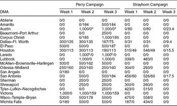
The timing and intensity of the television and radio ads in each DMA are depicted in Table 2. For example, the Victoria DMA received a full dose of 1,000 television GRPs from the first week on, whereas the Lubbock and Austin DMAs did so from week two on, and the Corpus Christi DMA received a burst of 1,000 GRPs only during the third week. Looking at the TV and radio trajectories in conjunction, we see a range of different configurations. In 13 DMAs there were periods during which TV ran in the absence of radio. In 4 DMAs, radio ran in the absence of broadcast TV. In 10 DMAs, the two ran concurrently during at least one week. Also noteworthy are weeks in which nothing aired: 11 DMAs aired no media during week 1; 4 were quiescent during week 2; and 2 DMAs ran no ads during week 3. After week 3, no ads were run in any media markets for the duration of the study.
Television and Radio Advertising Purchases, by Media Market, Week, and Campaign (Entries are TV GRPs/Radio GRPs)

a In weeks 2 and 3, the Perry campaign aired 10 radio GRPs on Christian-format stations. Including or excluding these GRPs has no material effect on the results presented below.
b Although Laredo was assigned to receive 1,000 GRPs, media buyers were only able to purchase 475. This issue is addressed in Table 4, where we use instrumental variables regression to correct for the disjunction between intended and actual GRPs.
As we noted earlier, the Strayhorn campaign was on television and radio in some but not all of the media markets into which the Perry ads were introduced. The right panel of Table 2 shows the location and temporal relationship between the Perry and Strayhorn ads. As might be expected, given random assignment, the graph makes clear that the Strayhorn ads bear little relationship to the placement and timing of the Perry ads in the 18 experimental markets. Sometimes her ads precede the Perry ads; in other cases, they run concurrently. Her ads were localized both geographically and temporally, leaving ample statistical leverage for differentiating the effects of the two campaigns competing communications.
In forming the data for our pooled cross-sectional time-series analysis, the state of Texas has been divided into media markets. We divide the time units into weeks, as the campaign purchased its GRPs on a weekly basis. The overall pattern of results is little affected by whether we operationalize time in terms of weeks, which was the unit of experimental assignment, or days.Footnote 8 The advantage of coarser time units is the ability to track opinion change more reliably, due to greater numbers of survey interviews.
SURVEY DESIGN
In light of the fact that the unit of assignment is the DMA, we sought to allocate our survey sample in a way that would make the most of the experiment's power. The basic strategy was to spread the surveys more or less evenly across each of the geographic units. By reweighting the data according to the probability of selection from the voter file, we can approximate the results that would have obtained for a simple random sample, and our results conform closely to the results from a concurrent poll based on a simple random sample from the voter file.Footnote 9
The survey itself was conducted by Advantage Inc., a firm that specializes in “voter identification” calls—which is to say, brief and inexpensive surveys. One of the practical innovations of this experiment was the use of this type of survey, which cost one-tenth as much as a conventional survey per completed interview, allowing approximately 1,000 completed interviews per day.Footnote 10 (See online Appendix D for more information about response rates by week and media market.) The polling firm and its callers were blind to the purpose of the study and to the deployment of Perry advertising; the scripts did not link the survey in any way to a political party or campaign. The calls were conducted only in English, which limits our ability to generalize beyond the population of English-proficient registered voters. According to the 2006 American Community Survey, 14% of the Texas population reported speaking English less than “very well.” According to the 2006 Current Population Survey, 2.3% of U.S. citizens residing in Texas reported that “Spanish is the only language spoken by all members of the household who are 15 years of age or older.” (The survey did not ask about other languages.) From these figures, we infer that English proficiency excluded roughly 5–10% of the Texas electorate from our survey. Because the ads themselves were aired in English, this sample restriction parallels the likely audience for the ads themselves.
After a brief introduction,Footnote 11 the first two questions assessed the favorability ratings of the two leading candidates, Perry and Strayhorn. (See online Appendix B for text.) The third question asked voters whom they would vote for if the election were held today. The fourth and final question on the survey instrument was rotated among three randomly selected alternatives. The first item in the rotation was designed as a manipulation check to assess whether, as expected, respondents in treatment areas were more likely to recall seeing Perry advertisements than respondents in control areas. One-third of survey respondents received this question. A parallel question asking about exposure to Strayhorn ads was directed to one-third of the sample. The final one-third of the sample were asked about their radio listening habits. Note that these concluding questions were asked after candidate preference, so that they would not contaminate the outcome measures. The survey contains no measures of slow-moving variables such as age, education, or group membership, as the influence of time-invariant variables is eliminated in the within-subjects analysis presented below.
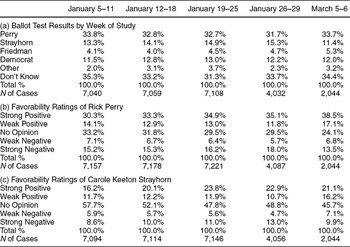
Table 3 describes statewide trends in public opinion. Although these trends do not speak to the question of advertising effectiveness, they provide a useful description of how the campaign unfolded in early 2006. The incumbent governor enjoyed a lead, but approximately one-third of the respondents declined to express a voting preference. As we move from the ballot test to candidate evaluations, somewhat stronger over-time patterns are apparent. During January, evaluations of Rick Perry became more polarized, with larger proportions of the sample offering strongly favorable or strongly unfavorable evaluations. Less pronounced but still noticeable is the week-by-week increase in the proportion of people who provide an evaluation. Evaluations of Carole Keeton Strayhorn were confined to a much smaller proportion of registered voters, as a large proportion of respondents conceded that they were unfamiliar with her. This proportion declined gradually, from 58% in the first week after she declared her candidacy to 49% three weeks later.
Survey Results over Time (Unweighted N)

Note: For question wording, see the supplementary online Appendix (http://www.journals.cambridge.org/psr2011005). Results here are unweighted for sampling probabilities, but weighted results are similar.
GAUGING THE EFFECTS OF BROADCAST TELEVISION AND RADIO
Our analysis is based on aggregate survey data, where the level of geographic aggregation is the media market and the level of temporal aggregation is the week (see online Appendix D). The resulting dataset contains 90 observations (N = 18 experimental media markets; T = 5 weeks, comprising three treatment weeks, one immediate follow-up week, and a long-term follow-up week five weeks later). For each DMA, we also have a pretreatment reading of voter preference during the days prior to the launch of the media campaign. Because the aggregate units encompass varying numbers of survey observations, the analyses below show how the results change when the data are weighted analytically to reflect the number of individual observations in each aggregate unit.
Within each randomization stratum,Footnote 12 we model the aggregate survey response as a linear function of the campaign's television and radio advertising, along with fixed effects for both time and geography:

In Equation (1), “TV GRPs” are weekly gross ratings points (in 1,000s) associated with Perry's TV ads, and “Radio GRPs” are weekly gross ratings points (in 1,000s) associated with Perry's radio ads. The dependent variable (Yit) is the percentage expressing an intention to vote for Perry (without excluding “don't know” responses).Footnote 13 The use of fixed effects for geography tracks a given DMA over time as ads are randomly rolled out; in effect, we have 18 distinct time series in which the media buy at any given time is randomly determined. Fixed effects for geography also have the virtue of controlling for regional differences in opinion caused by different survey response rates. The use of weekly fixed effects controls for statewide shocks that result from events or the vagaries of survey administration in any given week. When pooling all of the strata together into a single regression, we expand Equation (1) to include interactions between the weekly dummy variables and dummy variables marking each stratum.
An alternative modeling approach is to treat the δk parameters associated with each media market as random draws from a normal distribution. This random effects model uses fewer degrees of freedom and potentially generates more efficient estimates than the fixed effects model. Because DMAs are randomly assigned to treatments, the random effects are statistically independent of media exposure, which is a precondition for unbiased estimation. However, with just 18 experimental units, there is risk of correlation between the media treatments and the random effects, which can produce distorted estimates. In our experiment, the pretreatment measures of Perry support turn out to be negatively correlated with the television GRPs that were assigned to subsequent weeks. We present the random effects estimates, but suspect that they underestimate the effects of advertising.
One aim of this study is to examine the rate at which advertising effects decay. One way to study time-series dynamics is to introduce a lagged dependent variable as a regressor in Equation (1):

This specification is a nested alternative to Equation (1), in that the two are identical when ρ = 0. For 0 > ρ > 1, media effects decay geometrically in time, with larger values of ρ imply greater persistence in the effects of media advertisements. For example, if ρ were 0.5, TV GRPs would affect vote share by β 1 in the current week, by (0.5)β 1 in the subsequent week, (0.52)β 1 the week after, and so on.
As an alternative to the geometric decay model, we can also explore the time decay of ads using a variant of Equation (1) in which lagged media buys are included as regressors. A finite distributed lag model with a single lag, for example, augments the model in (1) by adding the preceding week's TV and radio GRPs:

Again, when pooling across randomization strata, we include interactions between strata dummies and week dummies to account for the fact that observations in different strata have different probabilities of being treated in each week (or in a previous week). Finally, a polynomial distributed lag (PDL) model operates on a principle similar to that in Equation (3) but sidesteps the problems of collinearity that result when multiple lags are introduced as regressors (Almon Reference Almon1965). The PDL specification constrains the lagged effects of a regressor to follow a polynomial equation.Footnote 14 We show below that the results of the PDL specification are robust for varying lag lengths and polynomial orders.
Each of these regression models may be augmented by including time-varying control variables. (Time-invariant control variables, such as pretreatment support for Perry in each market, are effectively included in the fixed effects model already, as they are perfectly predicted by the dummy variables for each media market.) Of particular interest are the radio and television GRPs purchased by the opposing Strayhorn campaign. Because the opponent's points were not randomly assigned, their causal effects are not identified. Including measures of Strayhorn's advertising nevertheless allows us to estimate the Perry ads’ effects while controlling for whatever incidental correlation might exist between the randomly assigned Perry ads and their nonrandomly assigned counterparts. In operational terms, this simply involves adding control variables to the equations above—something that turns out to have no real consequence for the estimated effects of the Perry ads. A further control variable is the average partisanship of a DMA. Partisanship is imputed based on the voter file, which indicates the number of Republican or Democratic primaries in which a person has voted. This pretreatment measure is a significant predictor of candidate preference at the individual level, and post-stratifying daily or weekly samples by partisanship dampens the sampling variability associated with our DMA-level averages of Yit.
RESULTS
This section begins by estimating simple models that ignore time-series dynamics and gradually builds up to more complex dynamic models. To preview the findings, we find relatively little evidence of time-series dynamics. Simple models, in other words, lead to roughly the same substantive conclusions as more elaborate models.
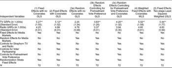
The columns of Table 4 show how the estimated effects of television and radio advertising change across alternative modeling approaches that do not involve dynamics. Table 4 focuses on the first four weeks of the advertising campaign. The first two columns report least-squares estimates with fixed effects for media market and week. Without covariates, the estimated effects of 1,000 GRPs of television and radio advertising are 5.27 (SE = 1.50) and 4.25 (SE = 5.91), respectively.Footnote 15 To put these estimates in perspective, it is helpful to bear in mind the fact that the campaign purchased up to 1,000 weekly GRPs of television advertising and 187 weekly GRPs of radio ads. The maximum dosage of television advertising apparently boosted Perry's relative standing by approximately six percentage points. Advertising thus appears to have the capacity to induce a substantial shift in vote preferences. The variance in radio advertising volume is much smaller, and the standard errors are therefore larger. We detect no significant effects of radio advertising, but this may reflect the much larger range of statistical uncertainty. As can be seen in column (2), the magnitude and statistical significance of the TV and radio coefficients remain largely unchanged when one introduces controls for the airing of opposing ads or the partisan composition of the sample.
Estimates of TV and Radio Advertising's Effects on Voter Preference, Measured Weekly

*p < .05.
**p < .01.
Note: Dependent variable is the percent of all respondents (including “don't know” responses) who, in a given DMA and in given week, favor Perry in a trial ballot. Partisanship is measured as the number of GOP primaries in which the voter has voted, minus the number of Democratic primaries. Specification (5) reports results from a weighted two-stage least squares regression (with a small-sample correction for the SE) in which the assigned TV GRPs and radio GRPs are used as instrumental variables for actual TV GRPs and radio GRPs.
The next three columns of Table 4 explore the consequences of altering the model to allow for random rather than fixed effects for each DMA. Without covariates, the estimated effect of television is smaller (2.25) and short of statistical significance. When we control for each DMA's level of Perry support prior to the start of the media campaign, the coefficient rises to 3.83 (SE = 1.26). Controlling further for partisanship and Strayhorn media raises the random effects estimate to 4.20 (SE = 1.32).
Specification (4) reports the results of a regression in which the data are weighted by sample size. The estimated effect of TV ads remains substantively unchanged when weights are applied. The coefficient (5.02, SE = 1.58) is very similar to the unweighted fixed effects estimate reported in column (2).
The final column in Table 4 represents the model that most closely reflects the nuances of the experimental design. The observations are weighted by sample size. Instrumental variables estimation is used to correct for the fact that in one of the markets, 1,000 TV GRPs were assigned but only 475 were actually aired, whereas in another DMA, 10 radio GRPs were aired when none were assigned. In this regression, randomly assigned GRPs serve as an instrument for actual GRPs (see Angrist, Imbens, and Rubin Reference Angrist, Imbens and Rubin1996). The results of this more exacting specification are similar to the other fixed-effects estimates in terms of magnitude and statistical significance. Overall, Table 4 shows that across a variety of model specifications and estimation methods, one generally obtains strong and significant effects of TV advertising, whereas the effects of radio advertising are properly signed but statistically indistinguishable from zero.
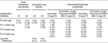
Table 5 shows how the estimated effects of TV and radio change when dynamic parameters are added to the fixed-effects model. To illuminate the way in which treatment effects decay, Table 5 includes data from week 9 of the study, roughly one month after the conclusion of the ad campaign. The regression models presented in columns (3) and (4) include a lagged dependent variable, as in Equation (2).Footnote 16 Comparing these columns to columns (1) and (2), which omit the lagged dependent variable, shows that the geometric lag specification has essentially no effect on the estimates. The lagged dependent variable turns out to be a weak predictor, with estimated ρ values that are statistically indistinguishable from zero. This pattern is not altogether surprising, because survey error in a relatively short weekly time-series attenuates the estimate of ρ. More interesting are the regression models that include lagged values of the media variables. Although including these lags introduces collinearity, thereby reducing our ability to estimate the effect of any particular lag with precision, the overall pattern is nonetheless suggestive. Television's effects appear to peak during the week in which the advertisements air. In column (1), for example, we see that the current week's advertising raises Perry's vote share by 4.73 percentage points per 1,000 GRPs (SE = 1.42); a week later, the effects of these ads have receded to −0.17 percentage points (SE = 1.42).Footnote 17
Dynamic Effects of Television Advertising on Voter Preference, Measured Weekly

Note: N = 90, except for specifications with lagged vote preference, for which N = 72. All models include fixed effects for week, DMA, randomization strata and lagged randomization strata. Finite distributed lag model (1) coincides with the “no covariates” specifications in Table 4, except that radio advertising has been omitted from the model. PDL models allow lagged effects of up to 3 weeks in duration, but models (6) and (8) impose the added constraint that cumulative effects go to zero after 4 weeks.
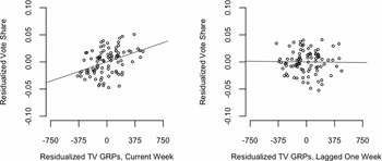
Figure 1 depicts the regression estimates in columns (1) and (2) to illustrate how television advertising boosts the sponsor when it is aired. The left panel plots residualized vote preference by residualized television GRPs aired in the current period. The graph suggests a strong and approximately linear relationship between TV exposure and voter preference. The right panel plots residualized vote preference by residualized television GRPs aired during the preceding week. The flat regression line illustrates the fact that advertising has a weak and statistically insignificant effect on voter opinion a week later.
Illustration of the Contrasting Effects of Current and Lagged TV Exposure, Weekly Data*

Turning to PDL models to assess the decay in effects over a longer time frame, we find a consistent pattern across the various specifications: TV ads exert a strong and significant effect in the current week, smaller and statistically equivocal effects a week later, and no effects thereafter. The only models to show significant effects of 1-week lags produce no evidence of lagged effects beyond 1 week.Footnote 18 Overall, the analysis of dynamics suggests that the effects of TV, although powerful, were short-lived. Not only did they dissipate before Election Day in November, they vanished before the March primary.
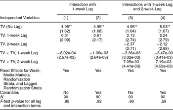
We can press the data a bit further in order to distinguish between decay and diminishing returns. Decay refers to the reduced influence of exposure over time, whereas diminishing returns refers to the idea that the influence of ads decreases with cumulative exposure to date. A straightforward way to test the diminishing returns hypothesis is to introduce an interaction between this week's ads and last week's ads:

A negative interaction (β3 < 0) is consistent with the diminishing returns hypothesis. The main effect of lagged GRPs (β2) gives a sense of how lagged exposure influences opinion when the current week's exposure is zero. The main effect of current GRPs (β 1) indicates the effect of “fresh” TV ads in markets where no ads have been shown previously. Table 6 presents the results of this analysis. Columns (1) and (2) interactions with a 1-week lag, and columns (3) and (4) interactions with both 1-week and 2-week lags. No evidence whatsoever is found for diminishing returns, and we again find evidence of strong short-term effects that decay rapidly. The same conclusions emerge when Table 6 is estimated using a random effects model, as in column (3c) of Table 4.
Assessing Whether the Effects of TV Diminish with Prior Exposure

*p < .05.
**p < .01.
The fact that opinion equilibrates quickly in the wake of a televised ad campaign such as the one studied here underscores the potential costliness of waging a battle for votes on TV. The immediate effect of a televised ad campaign makes it a cost-effective option in the short run. To shift opinion 5 percentage points among an electorate of 14 million people means persuading 700,000 voters. To expose the electorate to 1,000 GRPs of television at a rough average cost of $150 per point amounts to approximately $3 million per week. At less than $5 per vote, this expenditure is a bargain, but the difficulty is that there is little to show for one's money a week or two later.
DISCUSSION
Our study offers the first experimental estimate of campaign advertising's causal effects in a field setting. This research is not the first study to show advertising effects, but demonstrating these effects with a field experiment is an important advance because the research design sidesteps criticisms that are often levied against other research methods. The large effects observed in the laboratory are routinely challenged on the grounds that they fail to tell us how media exposure translates into votes in the context of an actual campaign, and rarely do scholars trace the over-time decay of lab-induced effects. The large effects found in observational studies are similarly open to the charge that campaigns target their ads strategically. Even when observational researchers have perfect measures of media exposure, they rarely have access to the inside information and strategic considerations that determine how a campaign allocates resources over time or space. In the gubernatorial campaign studied here, the volume, timing, and location of TV and radio ads were determined randomly.
The most provocative finding to emerge from this experiment concerns the rapid decay of advertising effects. With the important exception of the recent observational work by Hill et al. (Reference Hill, Lo, Vavreck and Zaller2010), very little attention has been given to the decay of advertising effects, and most previous research has ignored decay or implicitly assumed it is a much slower process than our findings suggest.
The rapid decay of advertising effects has important theoretical implications. In the course of a typical campaign, advertising targets are usually bombarded with messages without interruption; our experimental campaign enabled us to study how opinion equilibrates after the TV messages subside. This unusual design feature sheds light on the psychological mechanisms by which an ad designed to prime positive associations with the governor influences voter preferences.
Two basic psychological perspectives have dominated how scholars approach campaign effects. The first perspective emphasizes the information content of advertising. Recognizing that people forget the details of the information they receive, it has been argued that voters process information “on-line,” forming new opinions and then discarding the information on which those opinions were based. As Lodge, Steenbergen, and Brau (Reference Lodge, Steenbergen and Brau1995) argue, “memory for campaign messages not only fades but fades quickly . . . the half-life of the message typically being less than a week,” yet “recall is not a necessary condition for information to be influential” (pp. 315, 317–18). This interpretation has gradually won acceptance among public opinion scholars, who now concur that messages may have enduring effects even after their content is forgotten.
A second perspective is that advertisements prime voters to invoke different evaluative criteria when assessing candidates. An advertisement that stresses the threat posed by international terrorism might increase the extent to which voters draw on their foreign policy attitudes when evaluating presidential candidates. Iyengar, Peters, and Kinder (Reference Iyengar, Peters and Kinder1982) and Miller and Krosnick (Reference Miller, Krosnick, Mutz, Brody and Sniderman1996), for example, show that news stories have the capacity to strengthen the relationship between targeted attitude domains and candidate evaluations. Another argument with similar implications holds that the emotional content of advertisements accentuates their effects (Brader Reference Brader2005). The priming hypothesis implies that the effects of advertising decay as the cognitive accessibility of the primed considerations fades.
These two competing perspectives – learning and priming – have quite different empirical and theoretical implications that have not, to our knowledge, been integrated within a common theoretical framework. Although this is beyond the scope of the current paper, we have formalized a model that incorporates both types of effects.Footnote 19 Intuitively, from the standpoint of the rational learning model, a transitory advertising effect represents an anomaly. Rapid change is not in itself an anomaly, but to explain both rapid change in the wake of a commercial and rapid reversal of this change, one would have to posit that the information in the commercial contained a good deal of pertinent information to cause the initial change and that, subsequently, the outside environment happened to supply a comparable amount of pertinent information in rebuttal over the course of the next few days. This coincidence seems highly implausible given the uneventful way in which the campaign unfolded during the period of our study. An abrupt shift toward a candidate followed by a return to the prior state is, in contrast, compatible with an altogether different psychological process, akin to what Zaller (Reference Zaller1992) refers to as “sampling considerations.”
The pattern of results we observe suggests priming rather than on-line processing.Footnote 20 The precise way in which priming occurs is subject to alternative but complementary explanations. One possibility is that the ads made people more likely to place certain considerations in working memory. Another is that the ads increased the weight that people accorded these considerations when evaluating the candidates. Whether these ads jogged memory or focused attention or both, they do not appear to have propagated enduring beliefs.
The finding that campaign effects diminish sharply over time opens up a new research agenda. The theoretical arm of this broader research project involves formally characterizing the properties of different types of ads and the mechanisms through which they influence voter preference. Rational learning models are relatively well developed formally; more work needs to focus on formalizing propositions about memory, emotion, and attention that might account for the impact and dynamics of advertising.
This theoretical enterprise must be complemented by empirical exploration. Progress requires assessment of a range of different ads’ effects in different political contexts. Do the dynamics of opinion change look different when, instead of offering evocative imagery, an advertisement campaign reveals new information? Would, for example, a negative campaign ad that leveled a specific charge about an opponent's malfeasance in office produce an enduring shift in opinion? Do the effects of emotion-evoking ads dissipate more rapidly than ads with comparable content that lack emotional content? Are the effects of advertising muted toward the end of a campaign, when voters have acquired more information about the candidates, or do the priming or emotional mechanisms remain undiminished in influence?
As the empirical consequences of different types of ads come to be understood, scholars will be better positioned to develop arguments about the strategic logic of different types of advertising campaigns. The current study suggests that valence appeals have the capacity to influence large segments of the electorate, but although such ads may succeed in associating a candidate with a popular value in the short run, they face the challenge of presenting information that will have a lasting impact on the way that voters think about the candidates. Hard-hitting attack ads (e.g., charges of corruption) also appeal to valence dimensions, but may adduce evidence that has a more enduring impact on the way that a candidate is evaluated. From a strategic standpoint, the latter strategy seems riskier, which may explain why the incumbent front-runner studied here, who faced an array of challengers from across the ideological spectrum, chose to open his campaign with a positive broad-based appeal (Gerber Reference Gerber2004).
It should come as no surprise that a study such as this one generates as many research questions as it answers. This experiment is among the first in any discipline to estimate the effects of a large-scale media campaign using random assignment. At a minimum, this study must be replicated in other political contexts in order to answer basic questions, such as how much the effectiveness of advertising depends on the tone and content of the ads, proximity to Election Day, and the competitiveness of the race. In a similar vein, the relative effectiveness of radio and television advertising awaits further experimentation, given the limited power of the current study to detect radio's influence.
That said, the current study represents an important advance, both because it shows that large-scale experiments of this sort are possible and because it provides a reliable assessment of mass media's causal effects. Although, like any scientific effort, this study requires replication and refinement, the causal estimates it generates force a rethinking of several key topics in the field of political psychology. If campaign ads have powerful but short-lived effects on voter preference, what are we to conclude about the “minimal effects” thesis? It can hardly be said that people are so inattentive or resistant to new information that they fail to change, but on the other hand – consistent with models of priming or emotion but inconsistent with on-line processing – the effects of these messages appear to fade quickly. The advent of field experimental investigation of campaign advertising's effects, in sum, has the potential to profoundly shape the empirical foundation on which theories of political communication rest.




Comments
No Comments have been published for this article.