1 Introduction
The study of drop dynamics in the presence of external fields (e.g. electric, magnetic, acoustic or thermal) is gaining much importance nowadays due to the ease with which external fields can be used to manipulate drops in practical applications. External electric field is used in ink-jet printing, electrohydrodynamic (EHD) atomization, enhanced heat and mass transport processes, transport of fluids in microfluidic channels and so on (Teh et al. Reference Teh, Lin, Hung and Lee2008; Mhatre et al. Reference Mhatre, Vivacqua, Ghadiri, Abdullah, Al-Marri, Hassanpour, Hewakandamby, Azzopardi and Kermani2015; Anna Reference Anna2016; Ghasemi et al. Reference Ghasemi, Bararnia, Soleimanikutanaei and Lin2018; Poddar et al. Reference Poddar, Mandal, Bandopadhyay and Chakraborty2018, Reference Poddar, Mandal, Bandopadhyay and Chakraborty2019; Santra et al. Reference Santra, Sen, Das and Chakraborty2019).
In the present study, we are interested in investigating the effect of external electric fields on the gravitational settling of drops. A common application of gravity-induced motion of drops is the oil–water phase separation process in the oil industry (Eow, Ghadiri & Sharif Reference Eow, Ghadiri and Sharif2007; Berg, Lundgaard & Abi-Chebel Reference Berg, Lundgaard and Abi-Chebel2010; Mhatre et al. Reference Mhatre, Vivacqua, Ghadiri, Abdullah, Al-Marri, Hassanpour, Hewakandamby, Azzopardi and Kermani2015). Due to the presence of tiny drops and low density difference between oil and water, gravitational settling takes a long time. The separation efficiency can be enhanced by increasing the size of the drops, thereby enabling them to traverse faster (Berg et al. Reference Berg, Lundgaard and Abi-Chebel2010; Mhatre et al. Reference Mhatre, Vivacqua, Ghadiri, Abdullah, Al-Marri, Hassanpour, Hewakandamby, Azzopardi and Kermani2015). The former can be achieved by electro-coalescence (Eow et al. Reference Eow, Ghadiri, Sharif and Williams2001, Reference Eow, Ghadiri and Sharif2007; Berg et al. Reference Berg, Lundgaard and Abi-Chebel2010) of drops, while the drop settling speed can be increased significantly by applying external electric fields (Mhatre et al. Reference Mhatre, Vivacqua, Ghadiri, Abdullah, Al-Marri, Hassanpour, Hewakandamby, Azzopardi and Kermani2015).
Gravitational settling of drops is a classical problem of fluid dynamics with deformable fluid–fluid interfaces. Hadamard (Reference Hadamard1911) and Rybczynski (Reference Rybczynski1911) independently studied this problem and showed that, in the absence of fluid inertia, the drop remains spherical and moves vertically. Taylor & Acrivos (Reference Taylor and Acrivos1964), through singular perturbation analysis, studied the drop settling in the low Reynolds number regime. Their study showed that a drop deforms into an oblate shape while settling under gravity. Subsequently, several studies have been reported to bring out the gravity-driven dynamics of droplets, both experimentally (Hu & Kintner Reference Hu and Kintner1955; Klee & Treybal Reference Klee and Treybal1956; Wellek, Agrawal & Skelland Reference Wellek, Agrawal and Skelland1966; Wairegi & Grace Reference Wairegi and Grace1976) and numerically (Dandy & Leal Reference Dandy and Leal1989; Helenbrook & Edwards Reference Helenbrook and Edwards2002; Feng Reference Feng2010). Considering very high inertial stress as compared to capillary stress, Wairegi & Grace (Reference Wairegi and Grace1976) performed an experimental analysis for large drops and suggested the possibilities of various shapes (ellipsoidal cap, spherical cap, biconcave and toroidal). A relationship between terminal velocity and drop aspect ratio has also been calculated theoretically, which agrees well with their experimental results in the case of spherical caps. Dandy & Leal (Reference Dandy and Leal1989), using a finite difference scheme, studied the drag and deformation of settling drops for a large range of density and viscosity ratios. At low Reynolds number, they have observed a spherical cap, while the drop tends towards a disk-like shape at high Reynolds number. Extending the work of Dandy & Leal, later Helenbrook & Edwards (Reference Helenbrook and Edwards2002) performed extensive numerical analysis and reported two interesting shape evolutions of the drop (prolate and dimpled shape). Besides deformation, the drop terminal speed has been investigated explicitly by several researchers (Myint, Hosokawa & Tomiyama Reference Myint, Hosokawa and Tomiyama2006; Liu, Tang & Quan Reference Liu, Tang and Quan2013) for various fluid properties. Also, for rising bubbles, numerous studies have also been performed (Bhaga & Weber Reference Bhaga and Weber1981; Magnaudet & Eames Reference Magnaudet and Eames2000; Raymond & Rosant Reference Raymond and Rosant2000; Tripathi, Sahu & Govindarajan Reference Tripathi, Sahu and Govindarajan2015a ) which provide a useful physical insight into the dynamics of drop.
Application of an electric field significantly alters the drop dynamics. Electric field produces a Maxwell stress at the drop interface, the tangential component of which creates circulatory EHD flow in and around the drop. The normal component of the stress deforms the drop shape (Taylor Reference Taylor1966; Ajayi Reference Ajayi1978; Saville Reference Saville1997). Spertell & Saville (Reference Spertell, Saville and Plesset1974) first studied the effect of surface charge convection on the settling motion of a drop under a uniform electric field in the Stokes flow regime. Later, Xu & Homsy (Reference Xu and Homsy2006) performed an asymptotic analysis and compared the drop speed with their experimental data. Both the theoretical studies suggest alteration in drop speed due to surface charge convection and shape deformation. The asymptotic theory of Xu & Homsy (Reference Xu and Homsy2006) is limited to the small shape deformation and weak charge convection regime. To explore the regime of finite charge convection, recently, Yariv & Almog (Reference Yariv and Almog2016) performed an asymptotic analysis for a spherical drop and found a non-monotonic dependence of drop speed on the strength of charge convection.
A careful scrutiny of the reported literature shows that the effect of a uniform electric field on the gravitational settling of a drop has only been studied over a very small parameter regime, leaving the underlying rich fluid dynamics grossly unexplored. In practice, there are physical situations in which the drop can deform significantly and fluid inertia is not negligible. Moreover, surface charge convection coupled with inertial flow can bring noticeable alteration to the drop dynamics. Motivated by these considerations, here, we explore the EHD of a settling drop in the finite inertial regime using numerical simulations. To distinguish the effect of inertial forces, simulations are performed for weak and moderately strong inertial forces. Our results reveal that drop speed can be altered significantly on application of an electric field when the inertial force is relatively high. Fluid inertial not only affects the drop shape but also alters the surface charge convection, leading to the possible alteration of the drop trajectory in an intriguing manner.
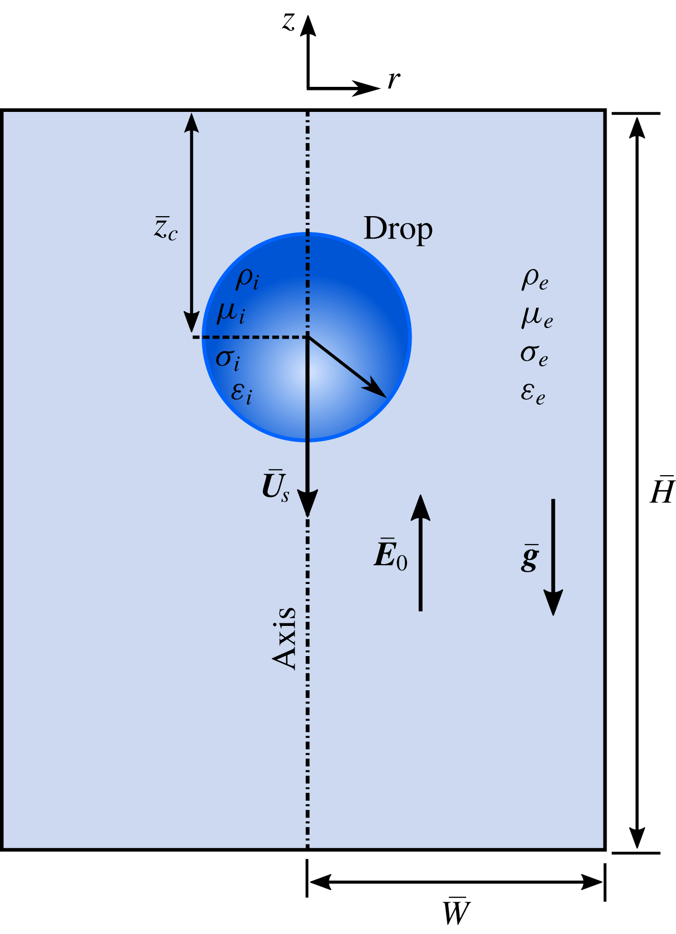
Schematic showing physical set-up used for numerical simulations. Drop of radius
 $a$
is placed at a vertical distance of
 $\overline{z}_{c}$
from top boundary in a domain of size
 $\overline{H}\times \overline{W}$
. Uniform electric field
 $(\overline{\boldsymbol{E}}_{0})$
is applied opposite to the direction of gravitational acceleration
 $(\overline{\boldsymbol{g}})$
.

2 Problem formulation
We consider a Newtonian drop of radius
 $a$
, suspended in another Newtonian medium (refer to figure 1 for schematic representation). Fluid properties such as density, viscosity, electrical permittivity and electrical conductivity are denoted by
 $\unicode[STIX]{x1D70C}$
,
 $\unicode[STIX]{x1D707}$
,
 $\unicode[STIX]{x1D716}$
and
 $\unicode[STIX]{x1D70E}$
, respectively. To distinguish drop phase and continuous phase, subscripts ‘i’ and ‘e’ are used. The difference in density assists the drop in settling under gravitational acceleration (
 $\overline{\boldsymbol{g}}=-\overline{g}\boldsymbol{e}_{\boldsymbol{z}}$
). Along with that, a uniform electric field,
 $\overline{\boldsymbol{E}}_{\mathbf{0}}=\overline{E}_{0}\boldsymbol{e}_{\boldsymbol{z}}$
, is imposed in the opposite direction to gravity to study the EHD of the setting drop. Under the combined action of buoyancy and an electric field, the drop settles with a terminal velocity
 $\overline{\boldsymbol{U}}_{S}=-\overline{U}_{S}\boldsymbol{e}_{z}$
. The interfacial tension between the drop and continuous phase is assumed to be uniform and denoted by
 $\unicode[STIX]{x1D6FE}$
. The drop dynamics is assumed to be symmetric about the z-axis. Note that a bar is used to denote dimensional variables.
2.1 Governing equations
Assuming both fluids as immiscible and incompressible, the continuity and momentum balance equations in the dimensional form are expressed as
 $$\begin{eqnarray}\displaystyle & \displaystyle \overline{\unicode[STIX]{x1D735}}\boldsymbol{\cdot }\overline{\boldsymbol{u}}=0, & \displaystyle\end{eqnarray}$$
 $$\begin{eqnarray}\displaystyle & \displaystyle \overline{\unicode[STIX]{x1D70C}}\left({\displaystyle \frac{\unicode[STIX]{x2202}\overline{\boldsymbol{u}}}{\unicode[STIX]{x2202}\overline{t}}}+\overline{\boldsymbol{u}}\boldsymbol{\cdot }\overline{\unicode[STIX]{x1D735}}\overline{\boldsymbol{u}}\right)=-\overline{\unicode[STIX]{x1D735}}\overline{p}+\overline{\unicode[STIX]{x1D735}}\boldsymbol{\cdot }\{\overline{\unicode[STIX]{x1D707}}(\unicode[STIX]{x1D735}u+(\unicode[STIX]{x1D735}u)^{\text{T}})\}+\overline{\boldsymbol{F}}_{\unicode[STIX]{x1D6FE}}+\overline{\boldsymbol{F}}_{E}-\overline{\unicode[STIX]{x1D70C}}\overline{g}\boldsymbol{e}_{\boldsymbol{z}}. & \displaystyle\end{eqnarray}$$
Here
 $\overline{\boldsymbol{u}}$
is the velocity field and
 $\overline{p}$
is the pressure. In (2.2)
 $\overline{\boldsymbol{F}}_{\unicode[STIX]{x1D6FE}}$
represents the surface tension force defined as
 $$\begin{eqnarray}\overline{\boldsymbol{F}}_{\unicode[STIX]{x1D6FE}}=\unicode[STIX]{x1D6FE}\overline{\unicode[STIX]{x1D705}}\boldsymbol{n}\overline{\unicode[STIX]{x1D6FF}}_{s},\end{eqnarray}$$
where
 $\boldsymbol{n}$
is the unit normal vector acting outwards at the interface,
 $\overline{\unicode[STIX]{x1D705}}=\overline{\unicode[STIX]{x1D735}}\boldsymbol{\cdot }\boldsymbol{n}$
is the curvature and
 $\overline{\unicode[STIX]{x1D6FF}}_{s}$
is the Dirac delta function. The effect of the electric field is incorporated into the momentum equation by the volumetric electrostatic force
 $(\overline{\boldsymbol{F}}_{E})$
expressed as
 $$\begin{eqnarray}\overline{\boldsymbol{F}}_{E}=\overline{\unicode[STIX]{x1D735}}\boldsymbol{\cdot }\overline{\unicode[STIX]{x1D749}}_{M}=\overline{q}_{v}\overline{\boldsymbol{E}}-{\textstyle \frac{1}{2}}\overline{E}^{2}\overline{\unicode[STIX]{x1D735}}\overline{\unicode[STIX]{x1D700}},\end{eqnarray}$$
where
 $\overline{\unicode[STIX]{x1D749}}_{M}=\overline{\unicode[STIX]{x1D700}}(\overline{\boldsymbol{E}}\overline{\boldsymbol{E}}-\frac{1}{2}\overline{E}^{2}\boldsymbol{I})$
is the Maxwell stress tensor,
 $\overline{\boldsymbol{E}}(=-\overline{\unicode[STIX]{x1D735}}\overline{\unicode[STIX]{x1D711}})$
is the electric field and
 $\overline{q}_{v}$
is the volumetric charge density. The electric field (
 $\overline{\boldsymbol{E}}$
) satisfies the Gauss law (Saville 1997)
 $$\begin{eqnarray}\overline{\unicode[STIX]{x1D735}}\boldsymbol{\cdot }(\overline{\unicode[STIX]{x1D700}}\overline{\boldsymbol{E}})=\overline{q}_{v},\end{eqnarray}$$
which can be expressed in terms of electric potential (
 $\unicode[STIX]{x1D711}$
) as
 $$\begin{eqnarray}\overline{\unicode[STIX]{x1D735}}\boldsymbol{\cdot }(\overline{\unicode[STIX]{x1D700}}\overline{\unicode[STIX]{x1D735}}\overline{\unicode[STIX]{x1D711}})=-\overline{q}_{v}.\end{eqnarray}$$
For perfectly dielectric fluids, as the charges are absent, equation (2.6) simply reduces to
 $$\begin{eqnarray}\overline{\unicode[STIX]{x1D735}}\boldsymbol{\cdot }(\overline{\unicode[STIX]{x1D700}}\overline{\unicode[STIX]{x1D735}}\overline{\unicode[STIX]{x1D711}})=0.\end{eqnarray}$$
For weakly conductive fluids, the volumetric charge density
 $\overline{q}_{v}$
is governed by the balance of ohmic conduction and convection of charges in the following form
 $$\begin{eqnarray}{\displaystyle \frac{\unicode[STIX]{x2202}\overline{q}_{v}}{\unicode[STIX]{x2202}\overline{t}}}+\overline{\unicode[STIX]{x1D735}}\boldsymbol{\cdot }(\overline{q}_{v}\overline{\boldsymbol{u}})=-\overline{\unicode[STIX]{x1D735}}\boldsymbol{\cdot }(\overline{\unicode[STIX]{x1D70E}}\overline{\boldsymbol{E}}).\end{eqnarray}$$
It is important to note that in the leaky dielectric model, the interacting fluids are considered to be free of volumetric charges (i.e.
 $\overline{q}_{v}=0$
), while the ohmic conduction across the fluid–fluid interface is balanced by a surface convection of charges (Melcher & Taylor Reference Melcher and Taylor1969; Saville Reference Saville1997). On the other hand, one may appeal to a more generic framework (as provided by the open-source code Gerris) and look into the transport of charges in terms of volumetric quantity. In the limit of small charge relaxation time scale, all the volumetric charges quickly reach the drop surface which effectively transforms (2.6) to the Laplace equation for an electric potential, and (2.8) simplifies to a surface transport equation. Thus, the leaky dielectric model is naturally recovered from the present EHD model (Herrada et al.
Reference Herrada, López-Herrera, Gañán-Calvo, Vega, Montanero and Popinet2012; Gañán-Calvo et al.
Reference Gañán-Calvo, López-Herrera, Herrada, Ramos and Montanero2018). Note that the equations in the above set are coupled to each other. The fluid flow equations are coupled to the electric field and charge density via the electrostatic force density (
 $\overline{\boldsymbol{F}}_{E}$
) term in the momentum equation, while the charge density and electric field are coupled to the fluid flow via the charge convection (the second term on the left-hand side of (2.8)).
2.2 Non-dimensionalization
Before performing numerical simulations, we non-dimensionalize the system by using the following characteristic scales: spherical drop radius a is chosen as the length scale,
 $\sqrt{\overline{g}a}$
is chosen as the velocity scale (Tripathi et al.
Reference Tripathi, Sahu and Govindarajan2015a
; Tripathi, Sahu & Govindarajan Reference Tripathi, Sahu and Govindarajan2015b
) and
 $\overline{E}_{0}$
is chosen as the scale for the electric field. Fluid properties are scaled by the respective properties of the suspending medium. Using the above scales the following dimensionless parameters can be obtained:
 $$\begin{eqnarray}\displaystyle \left.\begin{array}{@{}c@{}}\displaystyle Ga={\displaystyle \frac{\unicode[STIX]{x1D70C}_{e}\overline{g}^{1/2}a^{3/2}}{\unicode[STIX]{x1D707}_{e}}},\quad Ca={\displaystyle \frac{\unicode[STIX]{x1D707}_{e}\sqrt{\overline{g}a}}{\unicode[STIX]{x1D6FE}}},\quad M={\displaystyle \frac{a\unicode[STIX]{x1D700}_{e}{\overline{E}_{0}}^{2}}{\unicode[STIX]{x1D707}_{e}\sqrt{\overline{g}a}}},\quad Re_{E}={\displaystyle \frac{\unicode[STIX]{x1D700}_{e}}{\unicode[STIX]{x1D70E}_{e}}}\sqrt{{\displaystyle \frac{\overline{g}}{a}},}\\[12.0pt] \displaystyle \unicode[STIX]{x1D706}={\displaystyle \frac{\unicode[STIX]{x1D707}_{i}}{\unicode[STIX]{x1D707}_{e}}},\quad \unicode[STIX]{x1D70C}_{r}={\displaystyle \frac{\unicode[STIX]{x1D70C}_{i}}{\unicode[STIX]{x1D70C}_{e}}},\quad R={\displaystyle \frac{\unicode[STIX]{x1D70E}_{i}}{\unicode[STIX]{x1D70E}_{e}}},\quad S={\displaystyle \frac{\unicode[STIX]{x1D700}_{i}}{\unicode[STIX]{x1D700}_{e}}}.\end{array}\right\} & & \displaystyle\end{eqnarray}$$
The Galilei number Ga represents the ratio of the inertial force (generated due to gravity) to the viscous force, and the capillary number Ca represents the ratio of the viscous force to the surface tension force. The Masson number
 $M$
describes the relative strength of the electric stress compared to the viscous stress (Bandopadhyay et al.
Reference Bandopadhyay, Mandal, Kishore and Chakraborty2016; Mandal, Bandopadhyay & Chakraborty Reference Mandal, Bandopadhyay and Chakraborty2017), and the ratio of the charge relaxation time scale,
 $\overline{t}_{e}=\unicode[STIX]{x1D700}_{e}/\unicode[STIX]{x1D70E}_{e}$
, and the flow time scale,
 $\overline{t}_{f}=\sqrt{a/\overline{g}}$
, is defined as the electric Reynolds number (
 $Re_{E}$
). In (2.9)
 $\unicode[STIX]{x1D706}$
,
 $\unicode[STIX]{x1D70C}_{r}$
, R and S represent the viscosity ratio, density ratio, electrical conductivity ratio and electric permittivity ratio, respectively.
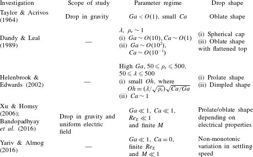
Summary of the past studies showing different drop characteristics for various parameter regimes.

Before proceeding further, we identify different parameter regimes which have been studied previously and summarize the drop characteristics in the respective regimes in table 1. Scrutinizing the details provided in table 1, it is clear that the shapes of buoyancy-driven drops are thoroughly investigated for a large range of Ga, Ca,
 $\unicode[STIX]{x1D706}$
and
 $\unicode[STIX]{x1D70C}_{r}$
in the absence of an electric field. Although the effects of an electric field on the drop motion and shape are investigated, the studies are limited to very small values of Ga. Hence, the EHD of settling drops in finite Ga regimes is investigated in the present study to explore the underlying fluid dynamics. However, a very high value of Ga can trigger the wake structure immensely (Dandy & Leal Reference Dandy and Leal1989; Tripathi et al.
Reference Tripathi, Sahu and Govindarajan2015b
). Under such circumstances, the drop shape and speed oscillate and in some cases even breakup has been observed (Tripathi et al.
Reference Tripathi, Sahu and Govindarajan2015b
). Here, we focus our attention on the flow regime with
 $Ga\sim O(10)$
, while Ca,
 $M$
and
 $Re_{E}$
are varied over a wide range. Physical properties from the experimental work of Hu & Kintner (Reference Hu and Kintner1955) (tetrachloroethylene drop suspended in water) are adopted for simulation purposes, which gives
 $\unicode[STIX]{x1D70C}_{r}=1.619$
and
 $\unicode[STIX]{x1D706}=1$
, while the electrical permittivity and conductivity are taken in such a way that behaviour of a wide range of perfectly dielectric and leaky dielectric fluids is recovered.
3 Numerical method
We use the open-source fluid flow solver Gerris which is developed by Popinet (Reference Popinet2003, Reference Popinet2009). The coupled EHD equations (as presented in the previous section) are solved using the finite volume method. To track the interface accurately, the volume of fluid (VOF) method is used in which the volume fraction (c) satisfies an advection equation of the form
 $$\begin{eqnarray}{\displaystyle \frac{\unicode[STIX]{x2202}c}{\unicode[STIX]{x2202}\overline{t}}}+\overline{\boldsymbol{u}}\boldsymbol{\cdot }\overline{\unicode[STIX]{x1D735}}c=0.\end{eqnarray}$$
The value of c is 1 inside the drop and 0 in the continuous phase. Density, viscosity, permittivity and conductivity of the fluids in dimensionless form are calculated using the weighted average mean method (López-Herrera, Popinet & Herrada Reference López-Herrera, Popinet and Herrada2011) as
 $$\begin{eqnarray}\displaystyle \left.\begin{array}{@{}c@{}}\unicode[STIX]{x1D70C}=c\unicode[STIX]{x1D70C}_{r}+(1-c),\quad \unicode[STIX]{x1D707}=c\unicode[STIX]{x1D706}+(1-c),\\ \unicode[STIX]{x1D700}=cS+(1-c),\quad \unicode[STIX]{x1D70E}=cR+(1-c).\end{array}\right\} & & \displaystyle\end{eqnarray}$$
Dynamic adaptive grid refinement is also employed, which allows us to use a very fine grid near the interface and a relatively coarse grid far from it, optimizing the computational time. Several reported studies have employed this solver for different EHD problems (López-Herrera et al.
Reference López-Herrera, Popinet and Herrada2011; Ferrera et al.
Reference Ferrera, López-Herrera, Herrada, Montanero and Acero2013; Cimpeanu, Papageorgiou & Petropoulos Reference Cimpeanu, Papageorgiou and Petropoulos2014) and obtained results with good accuracy. In the present study, an axisymmetric domain of height
 $\overline{H}$
and width
 $\overline{W}$
is considered, as shown in figure 1. The drop dynamics is assumed to be symmetric about the axis (shown by dash-dotted vertical line), while a Neumann boundary condition for flow field is imposed at all other sides of the domain. Except for the axis,
 $\overline{\unicode[STIX]{x1D711}}=-\overline{E}_{0}\overline{z}$
is specified at each boundary to simulate an upward uniform electric field. An axisymmetric boundary condition is imposed by setting the normal component of the velocity and the radial gradient of the electric potential and the tangential velocity component to zero (Sunder & Tomar Reference Sunder and Tomar2013) i.e.
 $\overline{u}_{r}=\unicode[STIX]{x2202}\overline{u}_{z}/\unicode[STIX]{x2202}\overline{r}=\unicode[STIX]{x2202}\overline{\unicode[STIX]{x1D711}}/\unicode[STIX]{x2202}\overline{r}=0$
, where
 $\overline{u}_{r}$
and
 $\overline{u}_{z}$
are velocity components in the r and z directions, respectively. To perform simulations, a domain of size
 $\overline{H}\times \overline{W}=60a\times 20a$
is considered. Initially, the drop is placed at a vertical location,
 $\overline{z}_{c}=10a$
from the top boundary so that the boundary has minimal effect on the drop motion. To capture the interface and charge convection accurately, a grid size of
 $\unicode[STIX]{x0394}\overline{r}=\unicode[STIX]{x0394}\overline{z}=\overline{W}\times 2^{-11}$
is taken near the interface whereas the bulk grid size is kept at
 $\unicode[STIX]{x0394}\overline{r}=\unicode[STIX]{x0394}\overline{z}=\overline{W}\times 2^{-5}$
. This numerical set-up is validated by performing comparisons with existing experimental, theoretical and numerical results (refer to appendix A for details). The details of the grid and domain independence studies are also provided in appendix B.
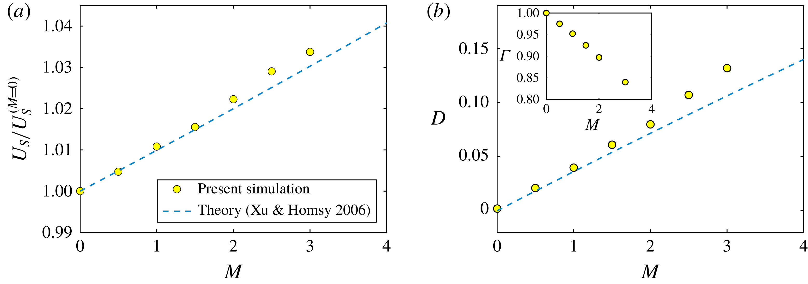
(a) Variation of normalized settling speed
 $(U_{S}/U_{S}^{(M=0)})$
with Masson number
 $M$
. (b) Variation of deformation D with Masson number
 $M$
for a PD drop considering
 $S=5$
,
 $Ga=1$
,
 $Ca=0.2$
and
 $\unicode[STIX]{x1D706}=1$
. Here
 $U_{S}^{(M=0)}(=0.1481)$
is the settling speed in the absence of an electric field. Inset of panel (b) shows the variation of cross-sectional area (
 $\unicode[STIX]{x1D6E4}$
) with
 $M$
.

4 Results and discussion
4.1 EHD of drop in the presence of weak inertia
Before investigating the EHD of a setting drop in the inertial regime, it is convenient to look into the effects of an electric field on the drop settling speed and drop deformation considering fluid inertia to be weak. To simulate the weak inertial regime, we consider
 $Ga=1$
and
 $Ca=0.2$
. To illustrate the effects of electric field strength on drop deformation and drop speed, we have considered two different drop-suspending media systems: (i) perfectly dielectric drop in a perfectly dielectric medium (PD–PD system) and (ii) leaky dielectric drop in leaky dielectric medium (LD–LD system). Figure 2(a) depicts the variation of drop speed with Masson number for a PD–PD system considering
 $S=5$
. To clearly represent the effect of the electric field, we plot the settling speed normalized by
 $U_{S}^{(M=0)}$
(which is the drop speed in the absence of an electric field for a specified Ga). A monotonic increase in drop speed is observed with an increase in Masson number. To explain this behaviour, we have shown the drop deformation for different Masson numbers in figure 2(b). Deformation of the drop is described by the deformation parameter
 $D=(L-B)/(L+B)$
, where L (or B) is the length of the deformed drop in the direction parallel (or perpendicular) to the applied electric field;
 $D>0$
represents prolate deformation (spheroidal drop shape with major axis parallel to electric field), whereas
 $D<0$
stands for oblate deformation (spheroidal drop shape with major axis perpendicular to electric field). Note that in the absence of an electric field (represented by
 $M=0$
), the drop remains in a spherical shape (
 $D=0$
) owing to the consideration of the weak inertial limit. In the presence of an electric field, a freely suspended PD drop always deforms into a prolate shape (
 $D>0$
) owing to the difference in permittivity (value of S other than 1) (Sherwood Reference Sherwood1988; Mandal et al.
Reference Mandal, Sinha, Bandopadhyay and Chakraborty2018). Similar behaviour is observed in the present case. In general, a prolate spheroid due to its shape travels with a higher speed than a sphere. This is due to the reduced cross-sectional area of the drop projected on a plane perpendicular to the direction of motion, which leads to a reduction in the hydrodynamic drag force and subsequent increase in drop speed. The variation of cross-sectional area (
 $\unicode[STIX]{x1D6E4}$
) normalized by the same for a sphere for various
 $M$
is provided in the inset of figure 2(b). Note that with the increase in Masson number, the electric stress is getting stronger against the capillary stress. This leads to an increase (or decrease) in deformation (or cross-sectional area) of the drop and subsequent increase in drop speed. To check the applicability of our numerical simulations, the normalized drop speed is compared with the theoretical results of Xu & Homsy (Reference Xu and Homsy2006) in figure 2(a). In the weak inertial regime (
 $Ga\ll 1$
), Xu & Homsy obtained the drop speed in the presence of a uniform electric field as
 $$\begin{eqnarray}U_{S}/U_{S}^{(M=0)}=1+CaM{\displaystyle \frac{3(3\unicode[STIX]{x1D706}^{2}-\unicode[STIX]{x1D706}+8)}{20(R+2)^{2}(3\unicode[STIX]{x1D706}+2)(\unicode[STIX]{x1D706}+1)}}\left[1+R^{2}-2S+3(R-S){\displaystyle \frac{3\unicode[STIX]{x1D706}+2}{5(\unicode[STIX]{x1D706}+1)}}\right].\end{eqnarray}$$
For a PD drop, the drop settling speed can be obtained by substituting
 $R=S$
in (4.1). By doing so, the term inside the square bracket can be obtained to be positive for an arbitrary value of S (other than 1). Hence, the drop speed always increases, as we also recover from simulations. Both for settling speed and deformation, our numerical results compare well with the theoretical results of Xu & Homsy (Reference Xu and Homsy2006) at a relatively small
 $M$
and show only a modest deviation on further increasing
 $M$
.
Next, we consider the EHD of the LD–LD system. Note that unlike the PD–PD system, the drop may deform into either prolate or oblate shape depending on electric property ratios (
 $R,S$
). For two different types of electrical parameters, variation of drop speed and deformation with
 $M$
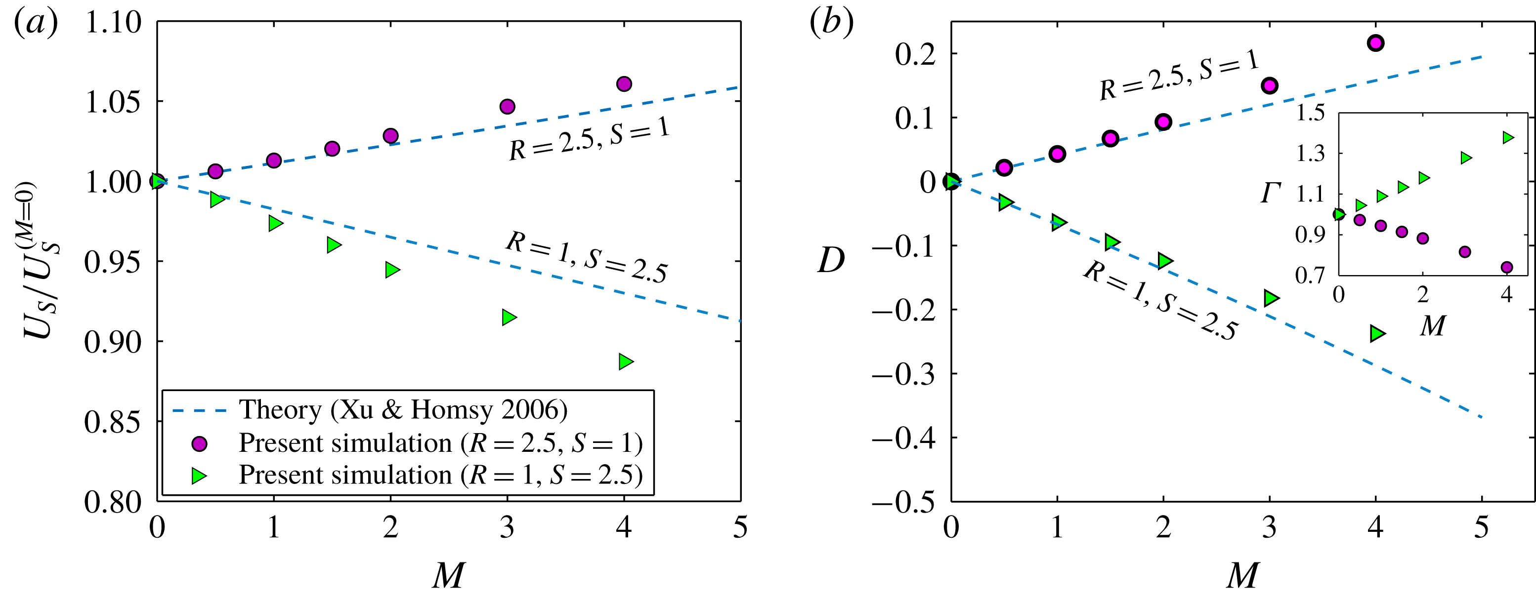
are shown in figures 3(a) and 3(b), respectively. It is observed that for
 $(R,S)=(2.5,1)$
, the drop speed increases monotonically, whereas for
 $(R,S)=(1,2.5)$
the drop speed falls on increasing
 $M$
. The different nature in the variation of drop speed is due to two different types of drop deformation, which are presented in figure 3(b). For more informative analysis, variation of normalized cross-sectional area (
 $\unicode[STIX]{x1D6E4}$
) with
 $M$
is provided in the inset of figure 3(b). For
 $(R,S)=(2.5,1)$
, the drop deforms into a prolate shape, which results in a decrease in
 $\unicode[STIX]{x1D6E4}$
and subsequent increase in drop speed. Whereas, for
 $(R,S)=(1,2.5)$
,
 $\unicode[STIX]{x1D6E4}$
increases owing to oblate shape and consequently the drop speed is reduced. As the inertial effects are very weak (
 $Ga=1$
), this allows us to employ Taylor’s discriminating function,
 $\unicode[STIX]{x1D719}_{T}=1+R^{2}-2S+3(R-S)(3\unicode[STIX]{x1D706}+2)/(5\unicode[STIX]{x1D706}+5)$
to compare the nature of drop deformation predicted by our results, where
 $\unicode[STIX]{x1D719}_{T}>0$
and
 $\unicode[STIX]{x1D719}_{T}<0$
defines the prolate and oblate deformations, respectively. It can be seen that for both (
 $R,S$
) combinations, our numerical model predicts the exact nature of deformation as Taylor’s discriminating function. A comparison between our numerical results and theoretical results of Xu & Homsy (Reference Xu and Homsy2006) is provided in figures 3(a) and 3(b). It can be observed that our results agree well with the asymptotic theory up to a moderate value of
 $M$
and show deviation with a further increase in
 $M$
. It is important to note that the theoretical model of Xu & Homsy is applicable only in the limit of small deformation. Beyond this limit, their theory either under predicts or over predicts as noticed in figure 3(a,b).
Variation of (a) normalized drop speed and (b) deformation parameter D with Masson number
 $M$
in case of a LD drop for different electrical property ratios. Other parameters taken are
 $Ga=1,Ca=0.2$
,
 $Re_{E}=0.01$
and
 $\unicode[STIX]{x1D706}=1$
. Inset of panel (b) shows the variation of cross-sectional area (
 $\unicode[STIX]{x1D6E4}$
) with
 $M$
for different electrical property ratios.

So far, we have seen that an electric field has a great influence on the drop shape and thereby can affect its motion. However, surface charge convection also plays a vital role in the alteration of drop shape as well as settling speed, as reported by previous investigations (Lanauze, Walker & Khair Reference Lanauze, Walker and Khair2015; Yariv & Almog Reference Yariv and Almog2016; Das & Saintillan Reference Das and Saintillan2017). Hence, before discussing the EHD behaviour of the drop in the high Ga regime, it is important to have a look on the effects of charge convection on drop speed in the low Ga regime. Note that the effect of charge convection is only present in case of LD drops as PD drops are free of charge. Following previous research works (Xu & Homsy Reference Xu and Homsy2006; Bandopadhyay et al.
Reference Bandopadhyay, Mandal, Kishore and Chakraborty2016; Yariv & Almog Reference Yariv and Almog2016), we parameterize surface charge convection by the electric Reynolds number (
 $Re_{E}$
). When
 $Re_{E}\rightarrow 0$
, the charge relaxation time scale is much smaller than the flow time scale (i.e.
 $\overline{t}_{e}\ll \overline{t}_{f}$
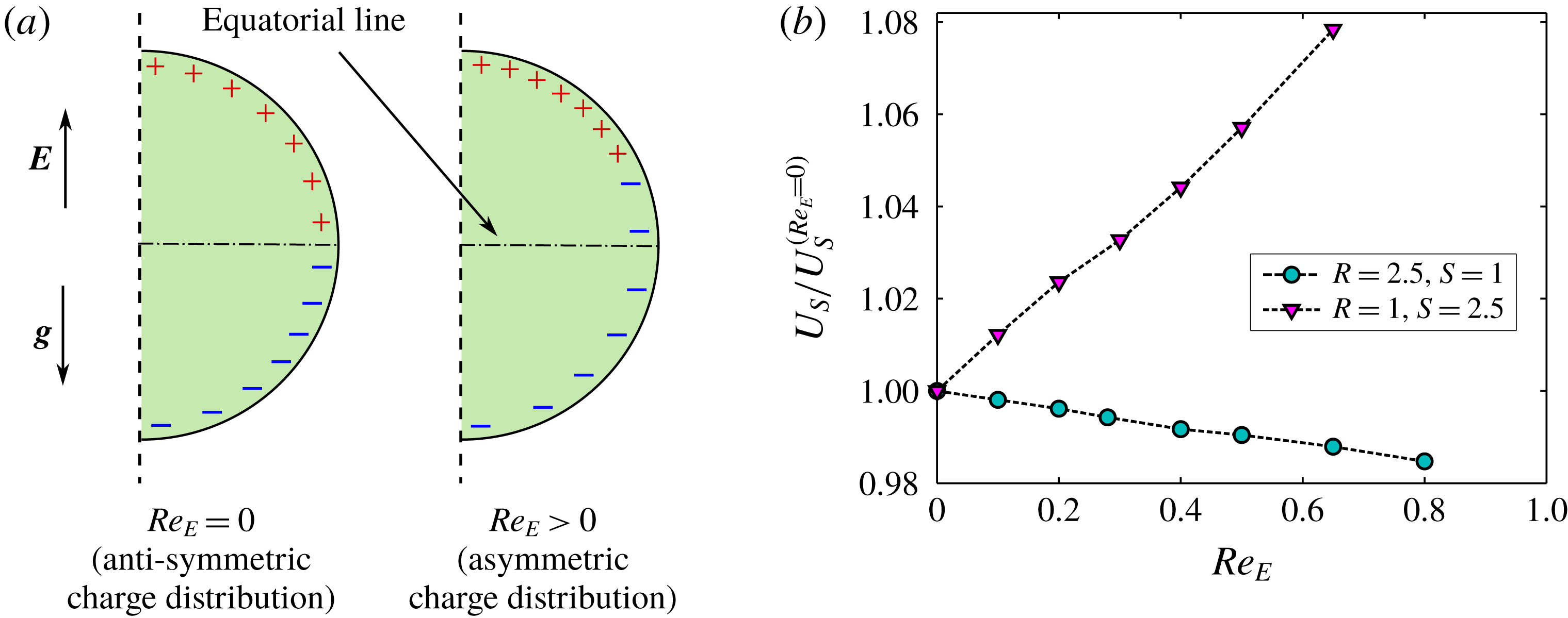
). Thus, the drop is polarized instantly and the charges are distributed in an anti-symmetric manner about the equatorial line, as represented schematically in figure 4(a). However, for non-zero
 $Re_{E}$
, the charges get transported by the fluid flow and redistributed in an asymmetric fashion. The above mentioned phenomenon generates an asymmetric tangential electric stress, which is balanced by the asymmetric hydrodynamic stress (Xu & Homsy Reference Xu and Homsy2006; Mandal et al.
Reference Mandal, Bandopadhyay and Chakraborty2017). The asymmetric hydrodynamic stress creates a net drag to the drop which may be positive or negative depending upon a discriminating parameter
 $G_{Re_{E}}=(R-S)(S-3R-3),$
found by previous analytical studies (Xu & Homsy Reference Xu and Homsy2006; Mandal et al.
Reference Mandal, Bandopadhyay and Chakraborty2017). The drop speed decreases (or increases) for
 $G_{Re_{E}}<0$
(or
 $G_{Re_{E}}>0$
). Figure 4(b) shows the variation of drop settling speed for two different (
 $R,S$
) combinations. For
 $(R,S)=(2.5,1)$
, a slower moving drop is observed on increasing
 $Re_{E}$
, which is due to the fact that
 $G_{Re_{E}}<0$
. For a different set of electrical properties i.e.
 $(R,S)=(1,2.5)$
,
 $G_{Re_{E}}$
is positive and accordingly an increase in the drop speed is observed, which is a sharp contrast to the previous case. With the increase in
 $Re_{E}$
, the surface charge convection continues for a longer time and results in more asymmetry in the charge distribution. Hence, for both the cases, a monotonic variation of drop speed with
 $Re_{E}$
is observed.
(a) Schematic showing surface charge distribution pattern for zero and non-zero
 $Re_{E}$
on a spherical drop for the case of
 $R>S$
. (b) Variation of settling speed with
 $Re_{E}$
for different electrical parameter ratios. Other parameters considered are
 $Ga=1,Ca=0.2$
,
 $M=4$
and
 $\unicode[STIX]{x1D706}=1$
. Here
 $U_{S}^{(Re_{E}=0)}$
is the drop speed in the absence of charge convection.

4.2 Combined influence of inertia and electric field on drop dynamics
Now we investigate the combined effects of gravity and a uniform electric field on the drop dynamics in the inertial flow regime, where the inertial force is relatively larger than the viscous force i.e. at a relatively higher Ga. The fluid properties considered are the same as the previous section. To avoid any instability in drop dynamics triggered by inertial forces, values of Ga up to O (10) are considered (Cano-Lozano, Bohorquez & Martínez-Bazán Reference Cano-Lozano, Bohorquez and Martínez-Bazán2013; Tripathi et al. Reference Tripathi, Sahu and Govindarajan2015a ).
4.2.1 PD–PD system
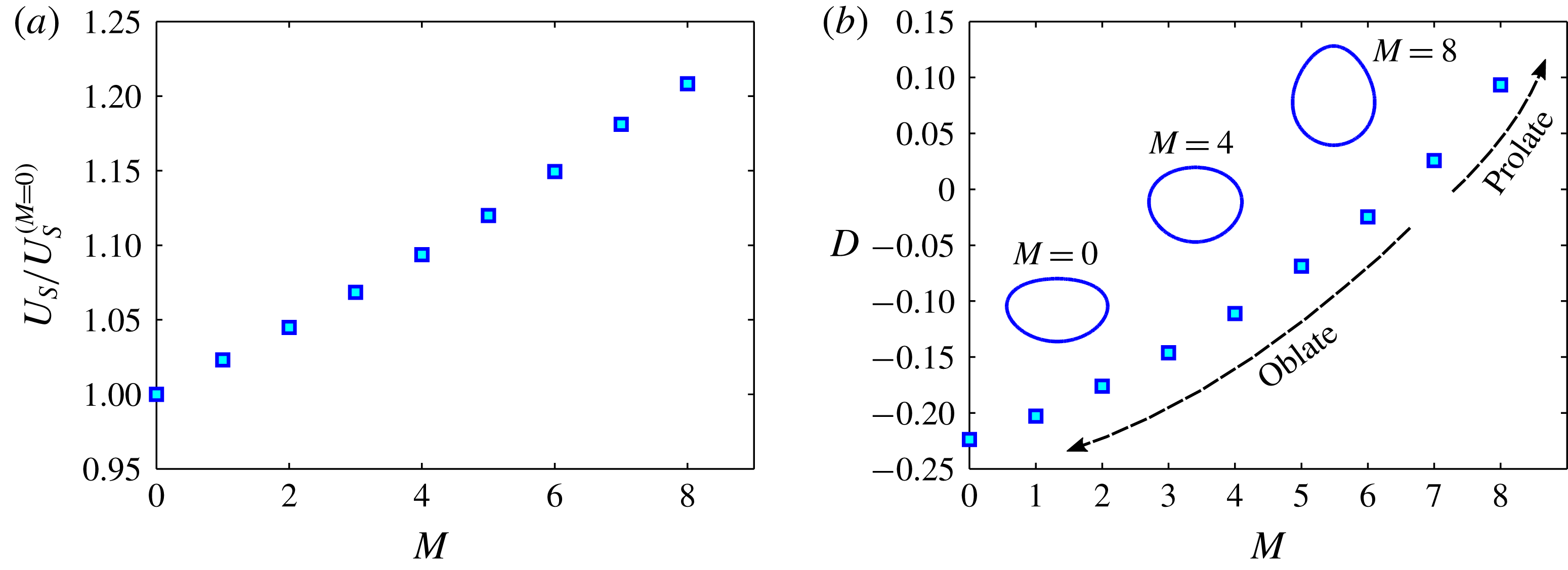
(a) Variation of normalized settling speed with Masson number
 $M$
. (b) Variation of deformation D with
 $M$
for a PD–PD system with
 $S=5$
. Other parameters used are
 $Ga=15$
,
 $Ca=0.2$
and
 $\unicode[STIX]{x1D706}=1$
. For
 $Ga=15$
, the value of
 $U_{S}^{(M=0)}$
is 0.8831. Inset of panel (b) shows the steady drop shapes for different
 $M$
values.

Figure 5(a) shows the variation of drop speed with Masson number of a PD drop for
 $S=5$
,
 $Ga=15$
and
 $Ca=0.2$
. Similar to the weak inertial regime, the drop speed increases with an increase in Masson number. Note that the rise in drop speed is almost linear. For a PD drop as the charges are absent, the modification in settling speed is attributed to deformation only. Variation of drop deformation with Masson number is presented in figure 5(b). For
 $M=0$
, the oblate drop shape is obtained due to the sole effect of fluid inertia. Note that a PD drop elongates in the direction of the applied electric field (prolate shape) in the weak inertial regime, as we have seen in figure 2(b). However, a settling drop can attain either a steady prolate or an oblate shape in the finite inertial regime. While the inertia promotes oblate deformation (Taylor & Acrivos Reference Taylor and Acrivos1964), the electric stress tries to elongate the drop in the direction of the electric field. Therefore, for a constant S and Ca, the steady-state shape of the drop is determined by the relative strengths of the electric stress and inertial stress i.e.
 $M/Ga$
. For a fixed Ga, the electric stress gets stronger against the inertial stress with an increase in
 $M$
. This is reflected in a gradual decline in oblate deformation; a more spherical drop shape is obtained. For the above considered parameters, it has been found that for
 $M=6.5$
(which gives
 $M/Ga=0.433$
) the electric stress is sufficient to balance the inertial stress and, as an outcome, the shape of the drop becomes approximately spherical. Subsequently, an increase in
 $M$
enhances the prolate deformation. In the inset of figure 5(b), the drop shapes for different
 $M$
are provided for better understanding. Further analysing the results, an important feature is noticed that for same values of Masson number the variation in deformation for a high Ga is less than the variation in deformation for low Ga. For the present set of parameters, varying
 $M$
from 0 to 3 changes the deformation
 $D=-0.2237$
to
 $D=-0.1462$
for
 $Ga=15$
, which is smaller than the change in deformation for
 $Ga=1$
(refer to figure 2(b)). This clearly indicates that the EHD deformation for a higher Ga is not a simple linear superposition of the drop deformations caused by the independent effects of buoyancy and electric field. Although, the change in D is less for the case of
 $Ga=15$
, the increase in settling speed is more, as compared to
 $Ga=1$
(refer to figure 2(a)). It is also important to mention that for
 $M=8$
, the increase in drop speed is substantially higher.
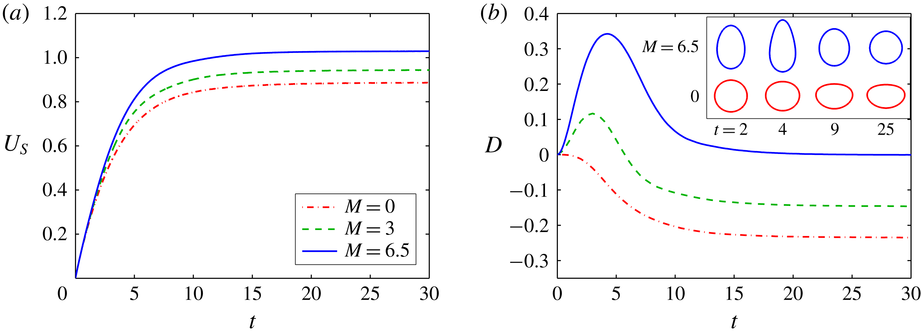
A more detailed understanding of the drop dynamics can be obtained if we look into the temporal evolution of drop speed and deformation. Figures 6(a) depicts the variation of settling speed with time (
 $t$
) for different values of
 $M$
. For
 $M=0$
, initially the settling speed varies at a faster rate, then gradually attains the steady value. For
 $M=3$
and 6.5, although the variation in
 $U_{S}$
looks qualitatively similar, however, it attains a higher steady-state value owing to deformation. Figure 6(b) depicts the transient variation in D for different
 $M$
. In the absence of an electric field (i.e.
 $M=0$
), a drop falling under gravity deforms into an oblate shape monotonically with time due to the influence of inertial stress. However, the combined presence of an electric field and fluid inertia brings about the non-monotonic transient behaviour in deformation. Note that for a PD drop the electric stresses are generated across the drop interface instantaneously, while the inertial stress is zero to start with as there is no flow at
 $t=0$
. With increase in time the drop gains speed and the inertial stress also increases. For
 $M=3$
and
 $M=6.5$
, it is observed that initially the drop deforms into a prolate shaped spheroid (
 $D>0$
) for
 $t<t_{MD}$
, where
 $t_{MD}$
refers to time required to achieve maximum deformation. For
 $M=3$
and
 $M=6.5$
, we obtain
 $t_{MD}=3$
and 4, respectively. Initially, the drop slowly gains motion, as shown in figure 6(a). It can be seen that the drop speed at
 $t\sim 2$
is sufficiently less as compared to the steady-state value. Hence, over the temporal regime,
 $t<t_{MD}$
, the deformation is mostly affected by electric stress rather than inertia generated stress. At
 $t=t_{ss}$
the drop attains steady state deformation. For all the cases, it is found that
 $t_{ss}\sim 25$
. Until at
 $t=t_{MD}$
, the drop gains sufficient velocity and hence, beyond this time limit (
 $t>t_{MD}$
) the inertial force comes into play. As a result, the drop deformation monotonically relaxes to a steady state value. A physical picture of the temporal evolution of drop shape for
 $M=0$
and
 $M=6.5$
is given in the inset of figure 6(b). For
 $M=3$
, the strength of the electric stress is not enough to balance the inertial stress, therefore the drop finally remains in an oblate shape. Whereas, for
 $M=6.5$
the EHD deformation is very high. Therefore, even after countered by the inertial stress, the drop attains a spherical shape at steady state. However, at a higher
 $M$
, the prolate drop shape can be obtained (refer to figure 5(b)). Interestingly, as we move to a higher value of
 $M$
, the deviation in D in the time limit
 $t_{MD}<t<t_{ss}$
becomes more. For
 $M=3$
and 6.5, the difference in D at
 $t=t_{MD}$
is significantly high, whereas at
 $t=t_{ss}$
the deviation is relatively less. To understand the physics behind such a fall in deformation we have to revisit into the transient variation of
 $U_{S}$
, presented in figure 6(a). Initially, the values of
 $U_{S}$
are almost the same. For finite
 $M$
, with an increase in deformation, the drop speed varies continuously afterward and attains a higher drop speed at steady state. As the inertial stress
 $\propto U_{S}^{2}$
, with the increase in
 $U_{S}$
with time, the magnitude of the inertial stress acting on the drop also start escalating. This elevated stress suppresses the EHD deformation more effectively. In the case of
 $Ga=1$
, the drop speed is very small (
 $U_{S}^{(M=0)}=0.1481$
) as compared to
 $Ga=15$
. Therefore, even after applying the electric field, the augmented speed (refer to figure 2(a)) fails to have any significant effect on drop deformation. From figure 6(b) it can be observed that at
 $t=t_{MD}$
, the drop is highly elongated. Hence, further increase in electric field may lead to shape instability followed by breakup.
Transient variation of (a) settling speed and (b) deformation for different values of Masson number
 $M$
for a PD–PD system with
 $S=5$
. Other parameters used are
 $Ga=15$
,
 $Ca=0.2$
and
 $\unicode[STIX]{x1D706}=1$
. Inset of panel (b) shows the drop shape comparison for
 $M=0$
and 6.5 at different times.

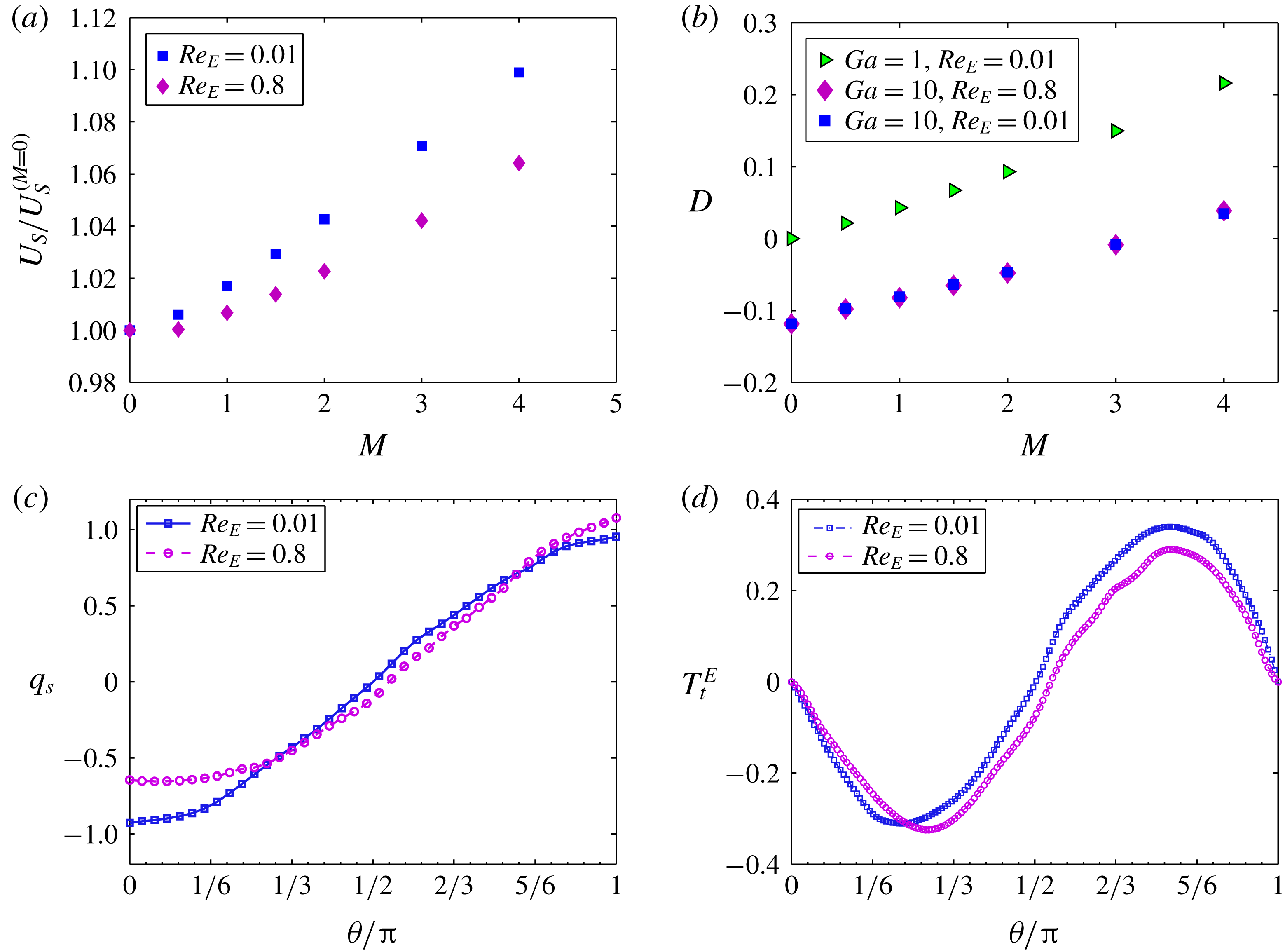
Variation of (a) normalized settling speed and (b) drop deformation D with Masson number
 $M$
for
 $R=2.5$
and
 $S=1$
. (c) Variation of steady-state surface charge density
 $q_{S}$
along the interface for
 $M=4$
. (d) Variation of steady-state tangential electric stress along the interface for
 $M=4$
. Other parameters considered are
 $Ga=10$
,
 $Ca=0.2$
and
 $\unicode[STIX]{x1D706}=1$
. For
 $Ga=10$
, the value of
 $U_{S}^{(M=0)}$
is 0.7884.

4.2.2 LD–LD system
Now we investigate the settling of a LD drop through a LD medium in the presence of an electric field considering
 $Ga=10$
and
 $Ca=0.2$
. First, we study the case where the electrical conductivity ratio is larger than the permittivity ratio (
 $R>S$
). For
 $(R,S)=(2.5,1)$
the drop speed increases with the increase in Masson number as depicted in figure 7(a). Interestingly, drop speed is less for
 $Re_{E}=0.8$
as compared to
 $Re_{E}=0.01$
. A similar phenomenon, albeit under the weak inertial limit, has been observed earlier (refer to §§ 4.1). On quantitative comparison, we found that in the case of
 $Ga=10$
, the alteration in drop speed due to charge convection is relatively high as compared to the case of
 $Ga=1$
. This may be due to the strong interfacial flow in the case of
 $Ga=10$
which transports the charges more efficiently and hence, a greater change in drop speed is observed. Figure 7(b) depicts the variation of D with
 $M$
for
 $Re_{E}=0.01$
and 0.8. It can be seen that for a LD drop with
 $R>S$
settling at
 $Ga=10$
, increasing the value of
 $M$
(hence
 $M/Ga$
) increases the resistance to oblate deformation, analogous to the case of a PD drop. For
 $M=3$
, the drop becomes almost spherical (
 $D=-0.0085$
). Further strengthening the electric field elongates the drop in the electric field direction. Results for
 $Ga=1$
are provided to explain the electric stress-dominated deformation. It is interesting to see that the charge convection has a weak effect on drop deformation for
 $(R,S)=(2.5,1)$
, so the scatters look indistinguishable. The insignificant effect of charge transport on prolate deformation was previously reported by Das & Saintillan (Reference Das and Saintillan2017) for neutrally buoyant drops. Hence, it is apparent that the alteration in drop speed for
 $Re_{E}=0.8$
is attributed to the asymmetry in electric stress produced by charge convection and not due to the change in deformation.
The variations of steady-state surface charge density (
 $q_{S}$
) and tangential electric stress (
 $T_{t}^{E}$
) along the interface are shown in figures 7(c) and 7(d) for
 $M=4$
to describe the alterations induced due to charge convection. In general, for a settling drop, both shape change and charge convection can break the anti-symmetry in
 $q_{S}$
and
 $T_{t}^{E}$
(Xu & Homsy Reference Xu and Homsy2006; Bandopadhyay et al.
Reference Bandopadhyay, Mandal, Kishore and Chakraborty2016; Mandal et al.
Reference Mandal, Bandopadhyay and Chakraborty2017). For
 $Re_{E}=0.01$
, an asymmetry (although very small) is observed in the variations of
 $q_{S}$
and
 $T_{t}^{E}$
. This is attributed to the asymmetric electric field in the vicinity of the drop interface, which is a result of the asymmetric drop shape. In the case of
 $Re_{E}=0.8$
, although D (hence the shape) remains almost the same, the asymmetry in charge distribution is quite significant. For
 $M=4$
and
 $Re_{E}=0.8$
, there is a fall in
 $q_{S}$
at
 $\unicode[STIX]{x1D703}=0$
(front end), whereas a rise in
 $q_{S}$
is observed at
 $\unicode[STIX]{x1D703}=\unicode[STIX]{x03C0}$
(rear end). In the presence of an electric field, the net flow is a combination of the EHD circulation and the flow due to settling (pole to pole) (Xu & Homsy Reference Xu and Homsy2006; Mandal et al.
Reference Mandal, Bandopadhyay and Chakraborty2017). Taking the example of a spherical drop (
 $Ca\ll 1$
), Yariv & Almog (Reference Yariv and Almog2016) explained that the EHD circulation is anti-symmetric about the equator (
 $\unicode[STIX]{x1D703}=\unicode[STIX]{x03C0}/2$
) and does not produce an asymmetric charge distribution. Hence, the asymmetry in
 $q_{S}$
is triggered by settling-induced circulation only. For the same reason, there is a fall in charge density at
 $\unicode[STIX]{x1D703}=0$
and augment at
 $\unicode[STIX]{x1D703}=\unicode[STIX]{x03C0}$
. The asymmetric charge distribution produces the tangential electric stress of similar nature (
 $T_{t}^{E}=q_{S}E$
) which consequently modifies the drag acting on the drop and hence alters the drop speed.
(a) Settling speed
 $U_{S}$
as a function of Galilei number Ga for different Masson numbers
 $M$
. (b) Deformation parameter D as a function of Ga for different
 $M$
. The inset of panel (b) shows steady-state drop shapes for various Ga and
 $M$
combinations. Other parameters considered are
 $R=2.5$
,
 $S=1$
,
 $\unicode[STIX]{x1D706}=1$
,
 $Ca=0.2$
and
 $Re_{E}=0.01$
.

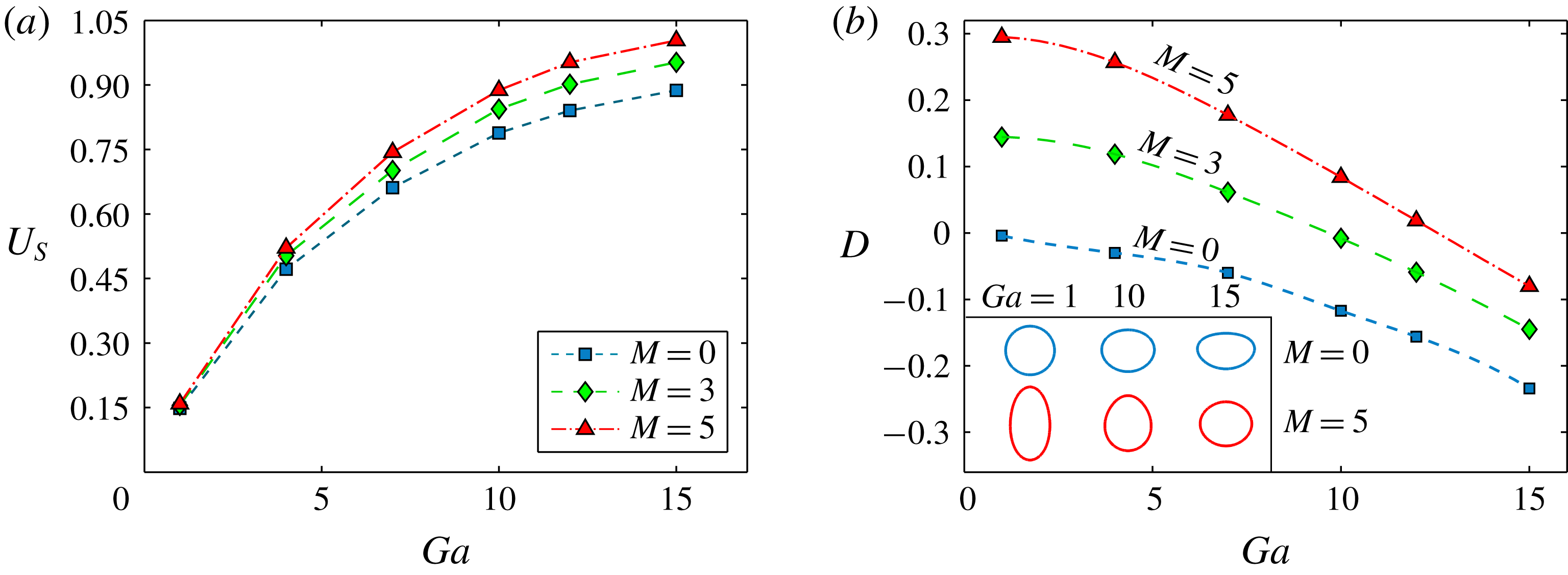
A common phenomenon observed from figures 5(b) and 7(b) is that the steady-state drop deformation is always less than the linear superposition of two independent deformations due to buoyancy and the electric field. To get more insight, simulations have been performed at various Ga neglecting the effect of charge convection. The variation of drop settling speed with Ga for various
 $M$
is depicted in figure 8(a). In general, for constant fluid properties (
 $\unicode[STIX]{x1D70C}_{r}$
,
 $\unicode[STIX]{x1D706}$
), an increase in Ga results in a higher drop speed in the absence of an electric field (
 $M=0$
) unless there is any large deformation (Hu & Kintner Reference Hu and Kintner1955). A similar trend with higher
 $U_{S}$
is observed for
 $M>0$
. The deviation in
 $U_{S}$
is very small at low Ga, hence less noticeable. However, at high Ga, the variation in
 $U_{S}$
is significant. Notably, the drop speed varies nonlinearly with Ga. Figure 8(b) shows the variation of D with Ga for different
 $M$
. For
 $M=0$
, by varying Ga to a higher value, the oblate deformation increases, which is attributed to higher inertial stress. As with the drop speed, the variation of D also shows a similar trend for
 $M>0$
. It is important to note that for a higher
 $M$
, D falls more rapidly with the change in Ga. To understand this phenomenon more physically, we have provided drop shapes at different Ga and
 $M$
combinations as the inset of figure 8(b). Varying Ga from 1 to 15, a substantial change in drop shape is observed for
 $M=5$
as compared to
 $M=0$
. The reason behind such behaviour is that for
 $M>0$
, the rise in drop speed at a higher Ga is larger, as discussed previously. This indicates that the change in inertia stress (
 $\propto U_{S}^{2}$
) due to application of an electric field is greater at a relatively high value of Ga. The elevated inertial stress resists the effect of electric stress more efficiently. As a consequence, the deformation versus Ga curves come closer as we move towards higher Ga.
Transient variation of (a) settling speed and (b) deformation for
 $R=2.5$
,
 $S=1$
. Other parameters considered are
 $Ga=10$
,
 $Ca=0.2$
and
 $\unicode[STIX]{x1D706}=1$
. The insets of panel (b) show drop shapes at steady state.

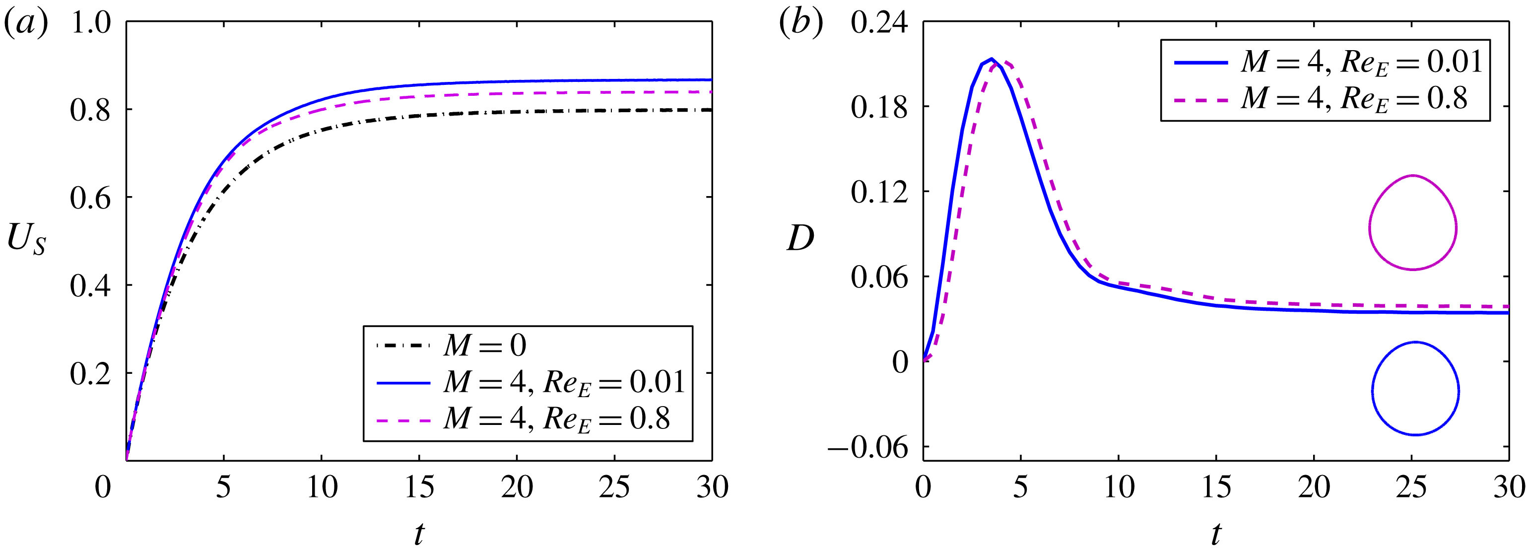
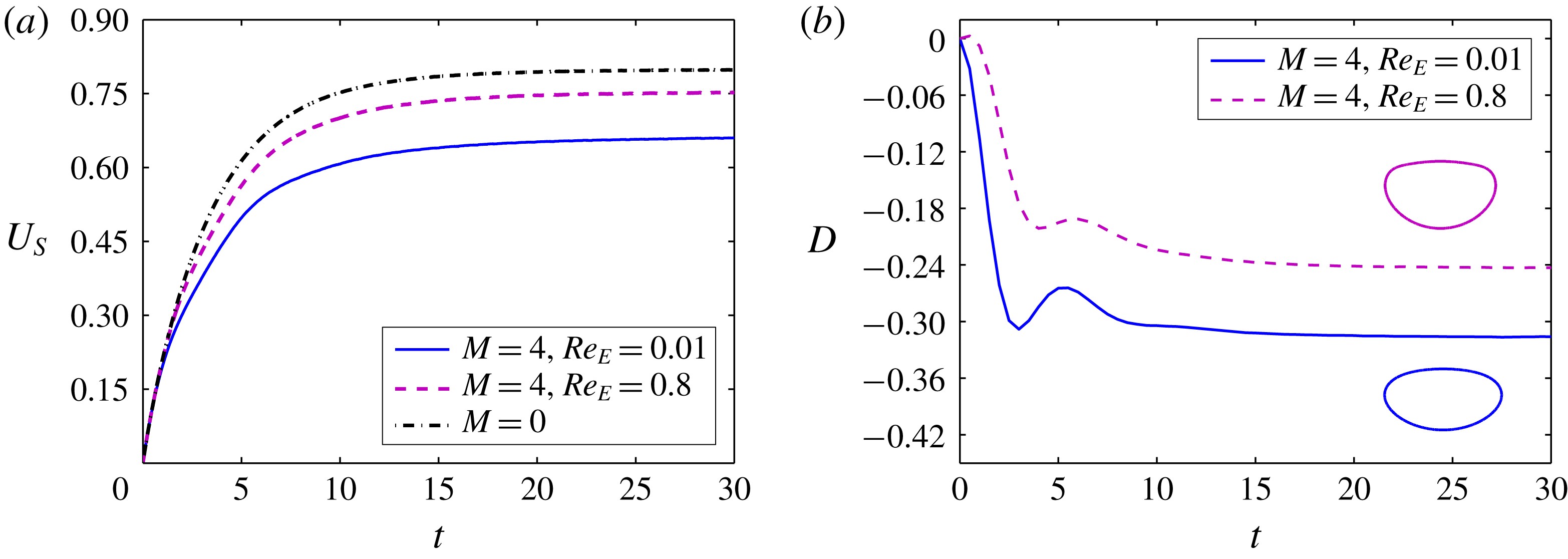
Now we discuss the effect of charge convection on transient behaviour of the drop. Figure 9(a) shows the variation of drop settling speed with time for
 $Re_{E}=0.01$
and 0.8. At the initial stage, the interfacial flow is weak, which makes charge convection ineffective. Hence, negligible variation in the drop speed is observed for
 $Re_{E}=0.8$
in this time limit. Afterwards, as the drop acquires enough motion, the strong interfacial flow starts redistributing the charges along the interface in an asymmetric manner. Consequently, the drop attains a lesser speed at steady state. Figure 9(b) shows the transient variation of deformation for
 $Re_{E}=0.01$
and 0.8. For
 $(R,S)=(2.5,1)$
, the variation of D is non-monotonic, similar to the case of the PD drop, as described earlier. For
 $Re_{E}=0.01$
, the drop gets polarized quickly. However, for
 $Re_{E}=0.8$
the charge relaxation time is comparatively high. This is the reason why
 $t_{MD}$
(time corresponding to maximum deformation) for
 $Re_{E}=0.8$
is more than that of
 $Re_{E}=0.01$
, as depicted in figure 9(b). Initially, the drop elongates in the flow direction up to
 $t=t_{MD}$
. In the time limit
 $t<t_{MD}$
, the inertial effects are small. Hence, Taylor’s discriminating function (
 $\unicode[STIX]{x1D719}_{T}$
) predicts the initial nature of deformation precisely. Afterward, the deformation decreases continuously to attain a steady-state value. When surface charge convection is taken into account, prolate drops deform more (Feng Reference Feng1999). Accordingly, for
 $Re_{E}=0.8$
, the drop shows additional deformation. Analogous to the PD drop, for
 $M=4$
the fall in D in the time limit
 $t_{MD}<t<t_{ss}$
is relatively higher than the deformation due solely to the effect of inertia (
 $M=0$
). This extra deviation in the case of
 $M=4$
is due to the augmented drop speed (as described earlier), which facilitates more oblate deformation.
Variation of (a) normalized settling speed and (b) deformation D with Masson number
 $M$
for
 $R=1$
,
 $S=2.5$
. (c) Steady-state volumetric charge density profile for
 $M=4$
. The parameters considered are
 $Ga=10$
,
 $Ca=0.2$
and
 $\unicode[STIX]{x1D706}=1$
. For
 $Ga=10$
, the value of
 $U_{S}^{(M=0)}$
is 0.7884.

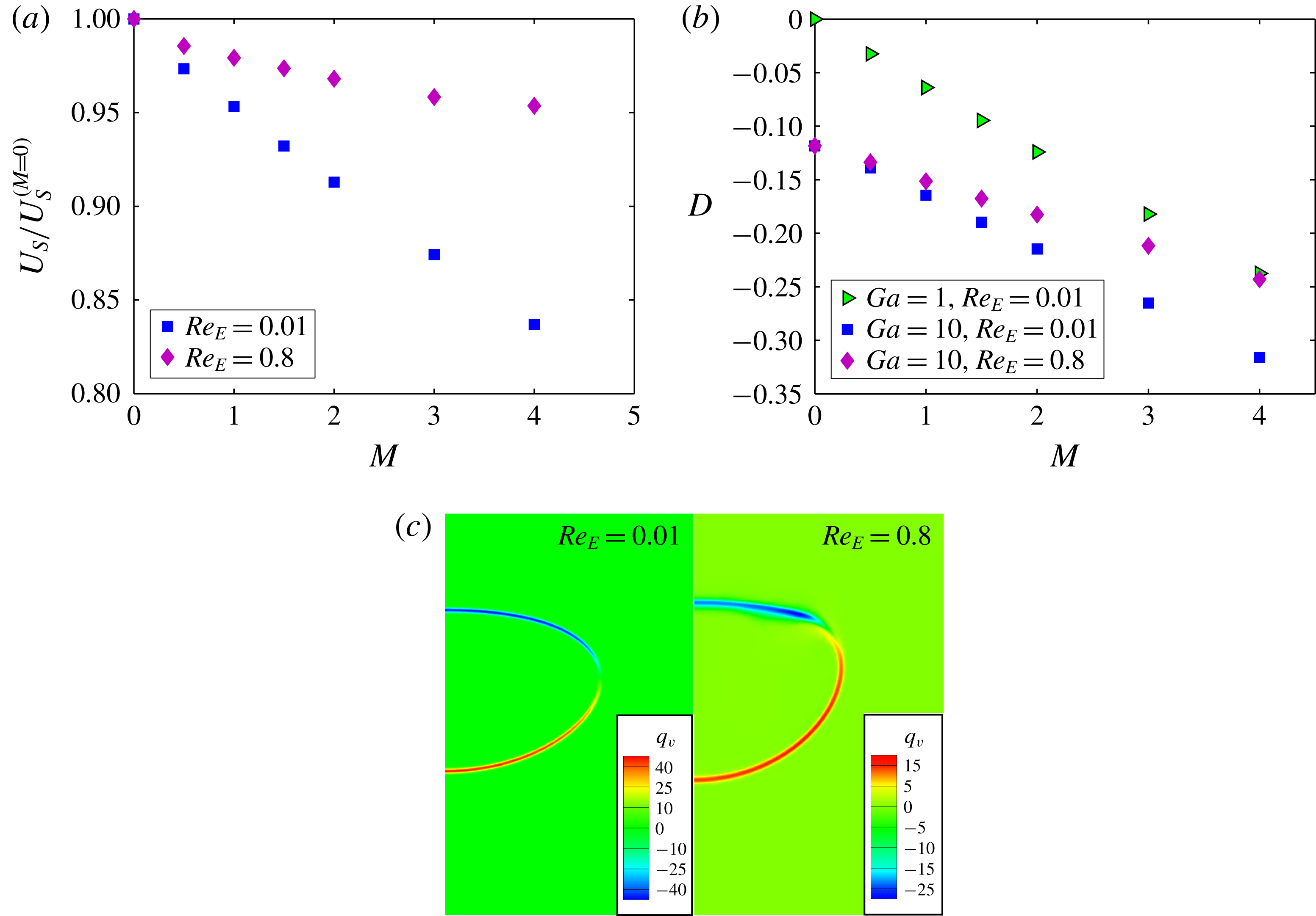
Next, we investigate a case in which the electrical conductivity ratio is less than the permittivity ratio (
 $R<S$
). Figure 10(a) depicts the variation of drop speed with Masson number for
 $R=1$
and
 $S=2.5$
. Drop speed decreases significantly with an increase in
 $M$
for
 $Re_{E}=0.01$
. For this choice of conductivity and permittivity ratio, the sole effect of electric stress is towards elongation of the drop in the transverse direction, reminiscent of the case with
 $Ga=1$
as shown in figure 10(b). Thus, the combined influence of electric and inertial stresses will distort the drop into a more oblate shape, which is also depicted in figure 10(b) for
 $Ga=10$
and
 $Re_{E}=0.01$
. Interestingly, the drop speed is quite high for
 $Re_{E}=0.8$
as compared to
 $Re_{E}=0.01$
(also noticed for
 $Ga=1$
). Note that for the reverse case i.e. when
 $R>S$
, the alteration in drop speed owing to charge convection is not that high, as seen previously. For
 $(R,S)=(1,2.5)$
, one reason behind such a large change in drop speed is the significantly less distorted oblate drop, as seen in figure 10(b). For a neutrally buoyant drop, charge convection reduces the oblate deformation, reported before by Feng (Reference Feng1999), Lanauze et al. (Reference Lanauze, Walker and Khair2015) and Das & Saintillan (Reference Das and Saintillan2017). Similar behaviour is observed by us in the inertial regime also. At
 $Ga=10$
and
 $M=4$
the steady-state deformation for
 $Re_{E}=0.8$
is very much less as compared to
 $Re_{E}=0.01$
. It is also important to note that for
 $(R,S)=(1,2.5)$
, the charge convection increases the drop speed due to the generation of an asymmetric electric stress despite no change in drop shape (Xu & Homsy Reference Xu and Homsy2006; Mandal et al.
Reference Mandal, Bandopadhyay and Chakraborty2017). The above phenomenon along with less distortion results in a large departure in drop speed. By looking into figure 10(a), it can be said that an increase in the electric field strength intensifies the effect of charge convection, resulting in more deviation. Figure 10(c) displays a typical volumetric charge density profile for
 $Re_{E}=0.01$
and 0.8 at steady state. For
 $Re_{E}=0.8$
the positive charges are distributed over a large surface and the negative charges are accumulated in a small region near the top surface, which confirms the asymmetric charge pattern about the equator. However, for
 $Re_{E}=0.01$
the opposite charges are allocated in a similar manner about the equator.
(a) Settling speed
 $U_{S}$
as a function of Galilei number Ga for different Masson numbers
 $M$
. (b) Deformation parameter D as a function of Ga for different
 $M$
. The inset of panel (b) shows steady-state drop shapes for various Ga and
 $M$
combinations. Other parameters considered are
 $R=1$
,
 $S=2.5$
,
 $\unicode[STIX]{x1D706}=1$
,
 $Ca=0.2$
and
 $Re_{E}=0.01$
.

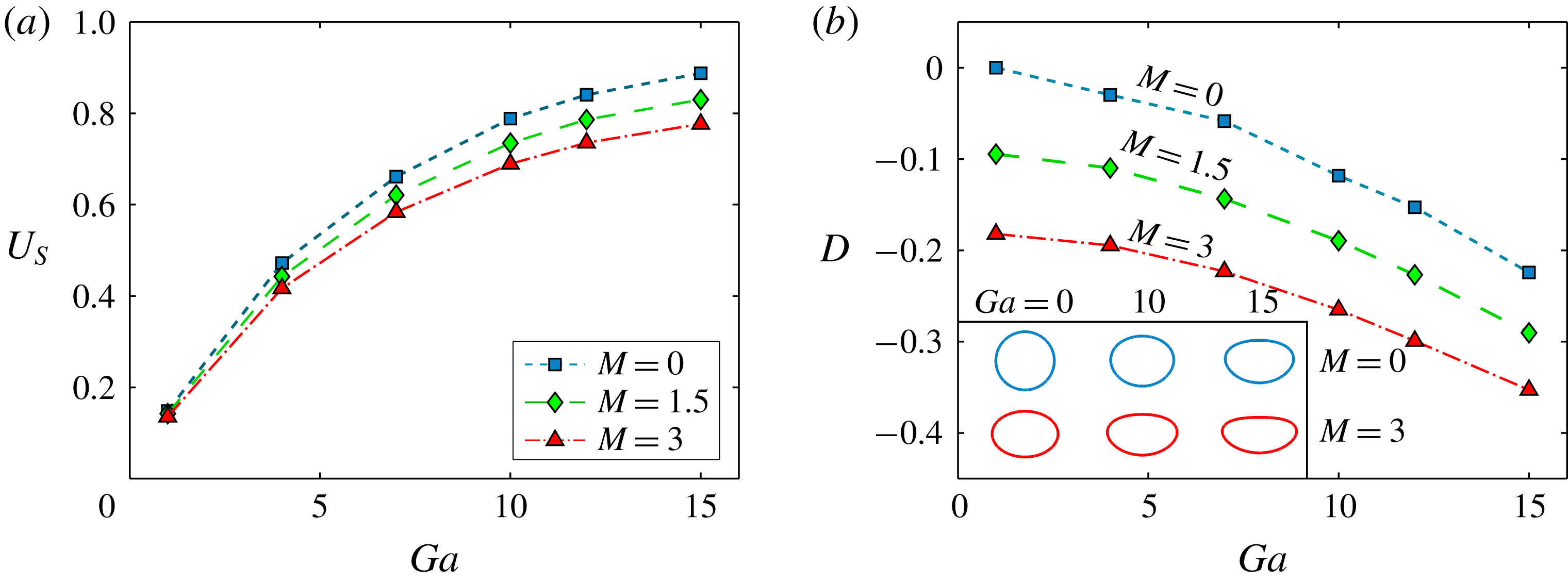
The effect of Ga on
 $U_{S}$
for various
 $M$
is presented in figure 11(a) considering
 $(R,S)=(1,2.5)$
. With increase in
 $M$
,
 $U_{S}$
falls due to an increase in cross-sectional area, as discussed previously. Moreover, at a higher Ga, this deviation is more prominent, similar to the case of
 $R>S$
. Figure 11(b) depicts the variation of D with Ga for different
 $M$
. The inset of the same figure shows the drop shapes for different Ga and
 $M$
values. At relatively higher Ga, the drop deforms into a more oblate shape owing to higher inertial stress. However, further investigation reveals that, with an increase in Ga, the deviation in D for
 $M=1.5$
and 3 is comparatively smaller than that for
 $M=0$
, which is in sharp contrast to the case of
 $R>S$
. For
 $R>S$
and
 $M>0$
, an increase in Ga results in an augmented drop speed. Whereas for
 $R<S$
, a lower drop speed is obtained in the presence of an electric field, as shown in figure 11(a). Consequently, the inertial stress (
 $\propto U_{S}^{2}$
) and its effect on deformation becomes weak. This is reflected in a gradual convergence (although slow for the present case) of curves as we proceed towards higher Ga. Notably, for
 $Ga=10$
and
 $M=4$
the combined deformation is less than the summation of individual deformations (refer to figure 10(b)).
Transient variation of (a) settling speed and (b) deformation for
 $R=1$
,
 $S=2.5$
. Other parameters considered are
 $Ga=10$
,
 $Ca=0.2$
and
 $\unicode[STIX]{x1D706}=1$
. The insets of panel (b) show drop shapes at steady state.

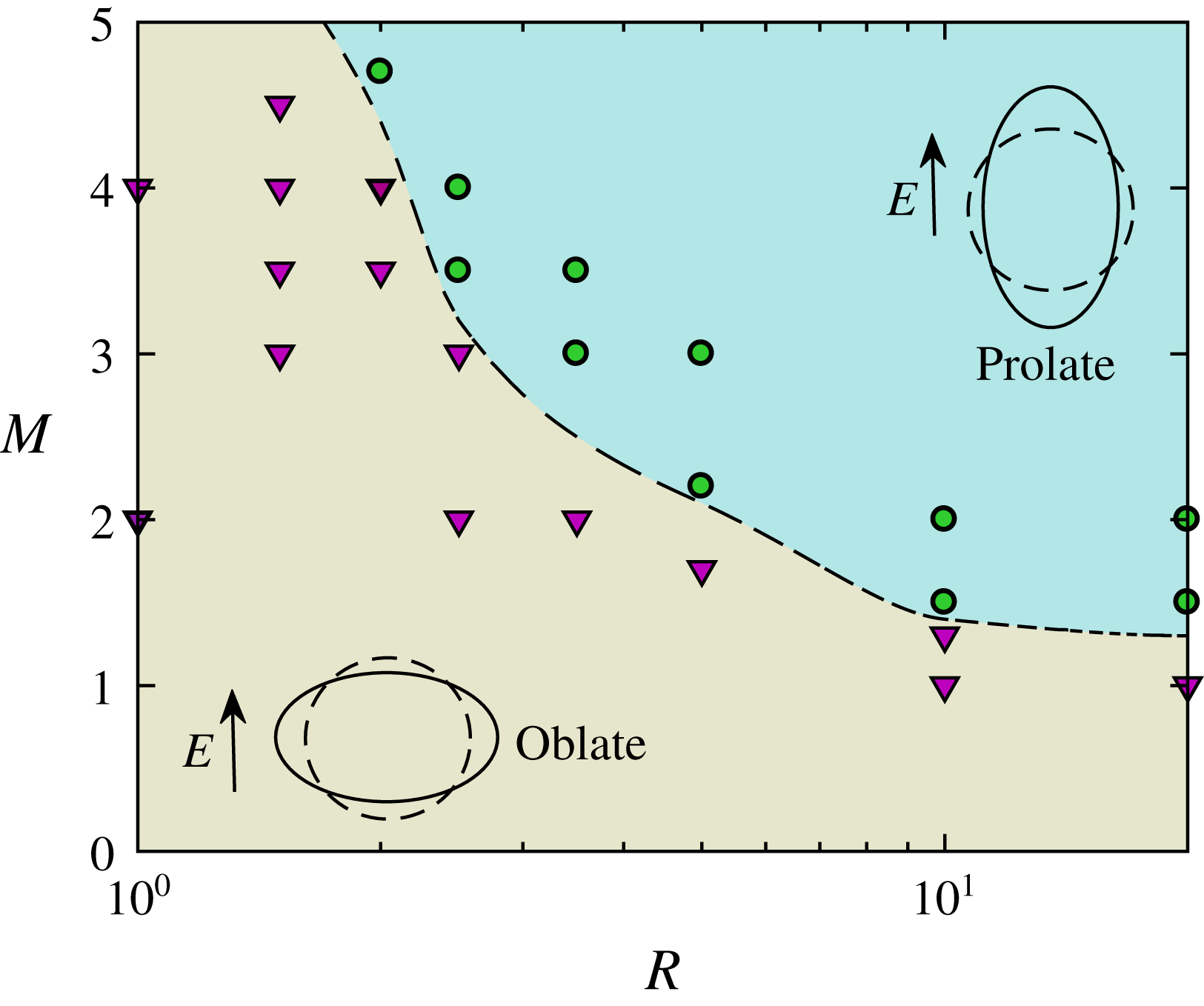
Regime diagram showing the shape of the drop in
 $M{-}R$
space. Other parameters considered are
 $S=1$
,
 $\unicode[STIX]{x1D706}=1$
,
 $Ga=10$
,
 $Ca=0.2$
and
 $Re_{E}=0.01$
.

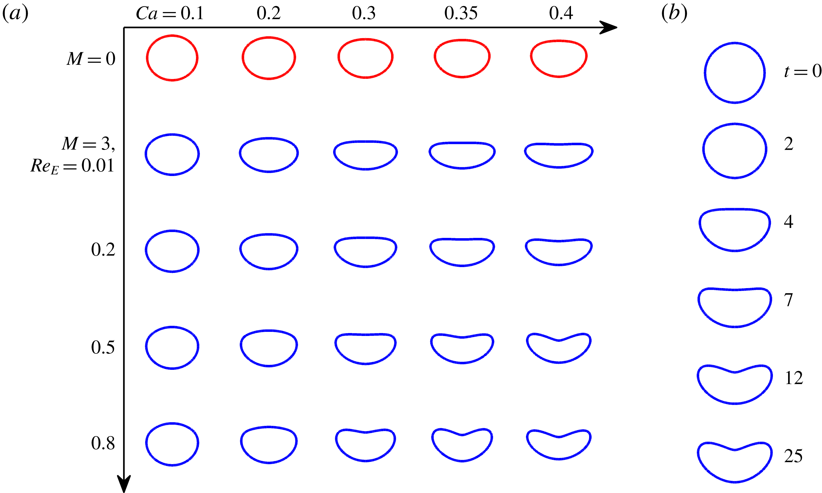
(a) Steady drop shapes for various combinations of Ca and
 $Re_{E}$
. (b) Evolution of drop shape with time for
 $Ca=0.35$
,
 $M=3$
and
 $Re_{E}=0.8$
. Other parameters considered are
 $R=1$
,
 $S=2.5$
,
 $\unicode[STIX]{x1D706}=1$
and
 $Ga=10$
.

Figure 12(a) shows the effect of charge convection on the transient variation of drop speed for
 $(R,S)=(1,2.5)$
. To support the discussion, transient variation of D is provided alongside in figure 12(b). For
 $Re_{E}=0.01$
, charges move to the interface quickly and the drop rapidly distorts into a highly oblate shape as the involved stresses are the same in nature. For this reason, after a small time
 $U_{S}$
starts diverging and the gradually acquires a much lower speed than the case of
 $M=0$
. Whereas in the case of
 $Re_{E}=0.8$
, the drop polarization time is high, reflected in a much slower deformation. Consequently, the deviation is drop speed is less as compared to
 $Re_{E}=0.01$
. For
 $(R,S)=(1,2.5)$
, the asymmetric electric stress generated due to charge convection results in less drag and a relatively less deformed drop as shown in the insets of figure 12(b). Hence, as the drop gradually acquires motion and the flow field triggers the charge transport, the drop starts settling with a substantially high speed as compared to
 $Re_{E}=0.01$
.
So far, we have observed the effect of
 $M$
on the drop deformation for different (
 $R,S$
) combinations. For
 $R<S$
, an oblate shape is the obvious outcome. However, for
 $R>S$
the nature of the deformation is a function of
 $M/Ga$
and
 $R/S$
considering other flow parameters to be constant. In figure 13, we present a regime plot in
 $M{-}R$
space for
 $S=1$
,
 $Ga=10$
and
 $Ca=0.2$
to explain the oblate to prolate transition in more detail. Although charge convection augments prolate deformation, the variation is very small, as shown in figure 7(b). Hence, to keep the discussion more general
 $Re_{E}=0.01$
is considered. For
 $(R,S)=(1,1)$
, the EHD deformation is zero (as
 $\unicode[STIX]{x1D719}_{T}=0$
) and independent of
 $M$
. For this case, the deformation is due to inertial stress only. In the
 $R>1$
region, the transition from oblate to prolate shape happens above a critical Masson number. By increasing the conductivity ratio, this critical value decreases, which is due to the fact that a higher value of conductivity ratio promotes more prolate deformation (Ajayi Reference Ajayi1978; López-Herrera et al.
Reference López-Herrera, Popinet and Herrada2011; Mandal, Bandopadhyay & Chakraborty Reference Mandal, Bandopadhyay and Chakraborty2016). However, for
 $R>10$
the critical value of Masson number remains nearly the same. This is due to the fact that for
 $R>10$
the drop behaves as a conducting drop. Subsequent increase in R does not change the EHD deformation much. For example, for
 $M=1.5$
, by increasing R from 10 to 20, the value of D deviates only by 0.005. Hence, the strength of electric field required to overcome the effects of inertial stress does not vary appreciably.
All the results presented above are obtained by performing simulations for a constant value of capillary number (Ca). However, variation in Ca can alter the deformation, both due to inertial stress as well as electric stress. For small values of Ga and
 $M$
, drop shape is less sensitive to change in Ca. However, at higher values of these parameters, a small change in Ca can drastically affect the drop shape. Along with inertia and the electric field, charge convection is also an important factor which can noticeably influence the drop deformation for a case of
 $R<S$
, as we have seen in § 4.2.2. Therefore, it may be interesting to see the interplay between the charge convection and drop deformability on the final drop shape. For
 $M=3$
and
 $Ga=10$
, we have presented steady-state drop shapes for various combinations of Ca and
 $Re_{E}$
in figure 14(a). For comparison, we have provided the drop shapes in the absence of an electric field in the top row of the figure. It can be observed that for
 $Re_{E}=0.01$
, with the increase in Ca the drop highly elongates in the transverse direction from the respective cases of
 $M=0$
. For
 $Ca=0.1$
and 0.2, both the top and bottom surfaces are almost equally rounded (i.e. less asymmetric). However, with the increase in Ca, the top surface becomes more flat. As a consequence, for
 $Ca=0.4$
the drop deforms into a disk-shaped structure. For
 $Ca=0.1$
, as we move in the direction of increasing
 $Re_{E}$
, the drop shape seems to be changed negligibly. However, in the case of
 $Ca=0.2$
, varying
 $Re_{E}$
from 0.01 to 0.8 results in much smaller deformation (shown previously in figure 10(b)). This shows that charge convection effects can only be noticeable only when the drop is highly deformable. Further increasing Ca to 0.3, a dimple is observed on the top surface of the drop at
 $Re_{E}=0.8$
. A similar drop characteristic has been reported before by Helenbrook & Edwards (Reference Helenbrook and Edwards2002) for a setting drop in the absence of an electric field. They have shown that, for a relatively small Ga and
 $Ca\sim O(1)$
, the viscous effects are very large, which results in the formation of a dimple. However, present results suggest that the dimpled shape can be obtained for much smaller Ca in the presence of charge convection. On further increase in Ca, we obtain dimpled shapes even for smaller
 $Re_{E}$
, as shown in figure 14(a). The reason behind such distortion is that charge transport alters the electric field in the vicinity of the drop. For the parameters considered, the charges move towards the top end (
 $\unicode[STIX]{x1D703}=\unicode[STIX]{x03C0}$
) by the interfacial flow. This results in higher charge accumulation (as shown earlier in figure 10(c)) and consequently a large jump in the normal component of the electric field across the interface at
 $\unicode[STIX]{x1D703}=\unicode[STIX]{x03C0}$
. This phenomenon significantly increases the normal component of electric stress (
 $(\unicode[STIX]{x1D749}_{M}\boldsymbol{\cdot }\boldsymbol{n})\boldsymbol{\cdot }\boldsymbol{n}$
) acting at the top end, as described previously by Sengupta, Walker & Khair (Reference Sengupta, Walker and Khair2017). Additionally, from the knowledge of flow over a sphere, the hydrodynamic pressure is maximum on the top and bottom ends (Helenbrook & Edwards Reference Helenbrook and Edwards2002; Feng Reference Feng2010). This combined effect of elevated normal electric stress and hydrodynamic pressure distorts the drop into a dimpled shape. Increase in Ca makes the drop more deformable. For this reason, the dimple looks more prominent at high Ca. The transient variation of drop shape is displayed in figure 14(b) for
 $Ca=0.35$
,
 $M=3$
and
 $Re_{E}=0.8$
. Initially, the electric field deforms the drop into an oblate shape followed by a shape with a flat top and rounded bottom. Once the drop attains a sufficient velocity, the charge convection becomes effective. Consequently, at
 $t=7$
, it is observed that the top surface is slightly dipped, whereas the bottom half still remains to be rounded. This depression grows with time and, finally, a more noticeable dimpled shape appears at steady state.
5 Conclusions
In the present work, the EHD of a settling drop is investigated under the combined action of a uniform electric field and gravity using numerical simulations. The effect of the interplay of inertial and electric forces on the steady and transient drop dynamics is studied, including surface charge convection. Simulations at low and moderate values of Galilei number are conducted to differentiate inertia-induced modifications in drop dynamics. Analysing the results, the following key conclusions can be drawn:
(i) In the weak inertial regime, the EHD of the drop is dominated by electric stresses. The speed of a perfect dielectric drop augments in the presence of an electric field owing to its prolate shape. In the case of a leaky dielectric drop, the deformation depends on the electrical properties of the fluids. The nature of the deformation obtained for low Galilei number is similar to that predicted by Taylor’s discriminating function
 $\unicode[STIX]{x1D719}_{T}(R,S,\unicode[STIX]{x1D706})$
. Increase in Masson number always results in a more distorted drop shape. In addition to drop deformation, drop speed is a function of charge convection when drop and medium fluids are leaky dielectric. Alteration due to charge convection depends on the electrical properties of the fluids. For prolate drops, charge convection reduces the drop speed. The nature of the alteration is in accordance with the reported theories.
(ii) Unlike the weak inertial regime, the steady drop shape of a perfectly dielectric drop settling under the combined influence of a uniform electric field and fluid inertia can be prolate or oblate depending on the relative magnitudes of the Masson number and Galilei number. When the strength of the electric field is small, the fluid inertia dominates the drop shape and makes it oblate. However, beyond a critical electric field strength, the drop attains a steady-state prolate shape. For a PD drop, a non-monotonic transient deformation is observed; initially dominated by electric stress followed by inertial stress. Increase in Masson number always increases the drop speed.
(iii) In the inertial regime, a LD drop with
$R>S$
shows deformation behaviour similar to a PD drop. Charge convection leads to a lesser drop speed. For
$R>S$
, the EHD deformation is weakly affected by charge convection. For
$R<S$
both the electric stress and inertial stress attempt to elongate the drop in the transverse direction, resulting in a more oblate deformation and resistance to drop motion. In the case of
$R<S$
, drop deformation is highly modulated by charge convection unlike
$R>S$
. For a moderately high
$Re_{E}$
, the drop shows slower deformation and attains substantially less steady-state deformation than that for the case with
$Re_{E}=0.01$
. Less deformed drop together with the asymmetric tangential stress greatly improves the drop speed. With the increase in electric field strength, the effect of charge convection gets intensified; hence drop deformation and settling speed show greater deviation.(iv) An interesting feature found in the present study is that the deformation under the combined action of inertia and electric field is less than the linear supposition of the individual deformations due to buoyancy and the electric field. Application of an electric field modulates the speed by altering the drop shape. This modified speed further affects the shape. To support this phenomenon, we have simulated the problem by varying the different parameters, and this phenomenon is found to be common to all the cases.
(v) For
$R<S$
, drop shape is highly sensitive to the capillary number as it amplifies the effect of both inertial as well as electric stress. By increasing the capillary number for zero electric Reynolds number, the drop shape can significantly transform from an almost axisymmetric oblate shape to a disk-like structure, whereas, a high electric Reynolds number can result in a dimpled shape. With further increase in capillary number, the same can be observed at a relatively small electric Reynolds number.


Acknowledgement
S.C. acknowledges the Department of Science and Technology, Government of India, for a Sir J. C. Bose National Fellowship.
Appendix A. Validation
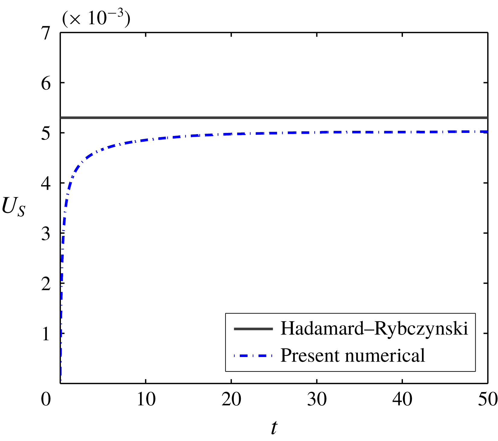
In figure 15, the settling speed (
 $U_{s}$
) is plotted against time (
 $t$
) for a drop falling with small
 $Ga$
and compared with the theoretically calculated terminal velocity by Hadamard (Reference Hadamard1911) and Rybczynski (Reference Rybczynski1911). Experimental data of Xu & Homsy (Reference Xu and Homsy2006) are used for simulation purposes. For a phenylmethylsiloxane-dimethylsiloxane drop (
 $\unicode[STIX]{x1D70C}_{i}=1000~\text{kg}~\text{m}^{-3}$
,
 $\unicode[STIX]{x1D707}_{i}=0.5~\text{Pa}~\text{s}$
) of radius 3.5 mm suspended in castor oil (
 $\unicode[STIX]{x1D70C}_{e}=957~\text{kg}~\text{m}^{-3}$
,
 $\unicode[STIX]{x1D707}_{e}=1.4~\text{Pa}\,\text{s}$
) with
 $\unicode[STIX]{x1D6FE}=5\times 10^{-3}~\text{N}~\text{m}^{-1}$
, the dimensionless parameters obtained are
 $Ga=0.445$
,
 $Ca=51$
,
 $\unicode[STIX]{x1D70C}_{r}=1.0406$
and
 $\unicode[STIX]{x1D706}=0.3571$
. The present numerical method predicts a velocity quite close to the analytically obtained settling velocity, as seen in figure 15. In the present case, the theoretical velocity is expressed as
 $U_{S}=(2/3)Ga(\unicode[STIX]{x1D70C}_{r}-1)((1+\unicode[STIX]{x1D706})/(2+3\unicode[STIX]{x1D706}))$
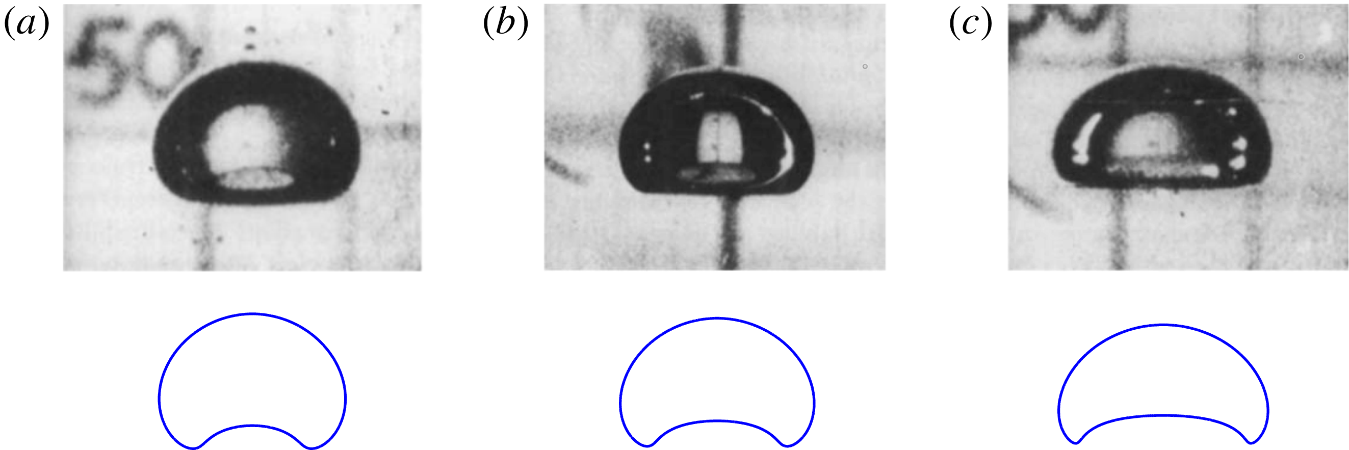
. To show the performance of the numerical code in the inertial regime, the steady-state shapes of the rising bubble obtained by our simulations for different combination of Ga and Ca are compared with the experimental results of Bhaga & Weber (Reference Bhaga and Weber1981) in figure 16. Numerically obtained drop shapes are shown at the bottom of figure 16. It is evident that the distorted shape of the bubble is well captured by our numerical scheme. The experimentally calculated values of Reynolds numbers (Re) are 2.47, 3.57 and 7.16, whereas numerically obtained values of
 $Re(=U_{S}Ga)$
are 2.49, 3.84 and 7.28, respectively.
Transient variation of drop velocity considering
 $Ga=0.445$
,
 $Ca=51$
,
 $\unicode[STIX]{x1D70C}_{r}=1.0406$
and
 $\unicode[STIX]{x1D706}=0.3571$
(using experimental data from Xu & Homsy (Reference Xu and Homsy2006)).

Comparison of numerically obtained steady-state bubble shapes rising in water with Bhaga & Weber (Reference Bhaga and Weber1981) for (a)
 $Ga=2.316$
,
 $Ca=12.55$
(b)
 $Ga=3.094$
,
 $Ca=9.373$
and (c)
 $Ga=4.935$
,
 $Ca=5.876$
.

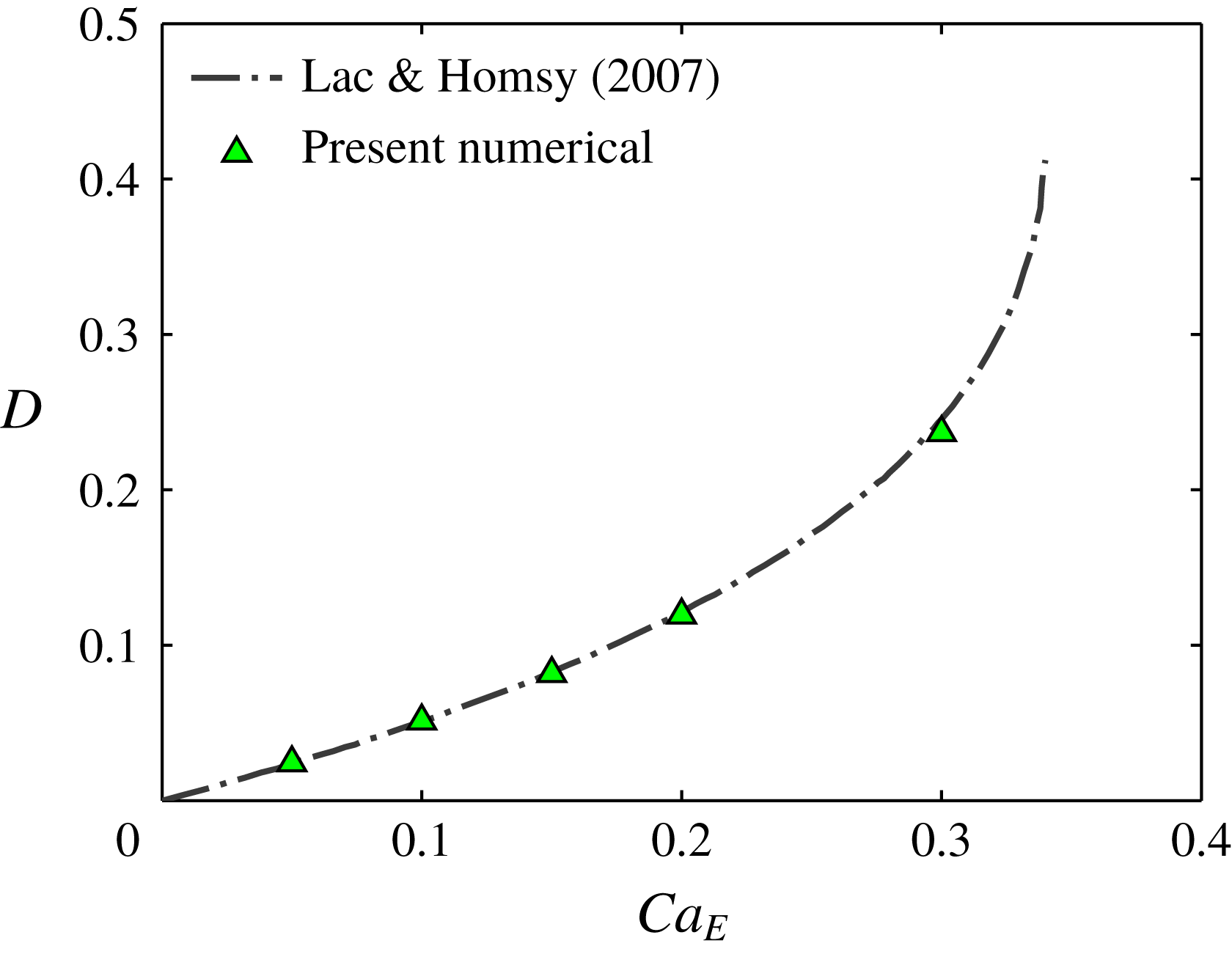
Variation of deformation of a neutrally buoyant drop with electric capillary number for
 $R=10,S=0.1$
and
 $\unicode[STIX]{x1D706}=1$
.
 $Ga=0.01$
and
 $Re_{E}=0.01$
are used for the present simulation.

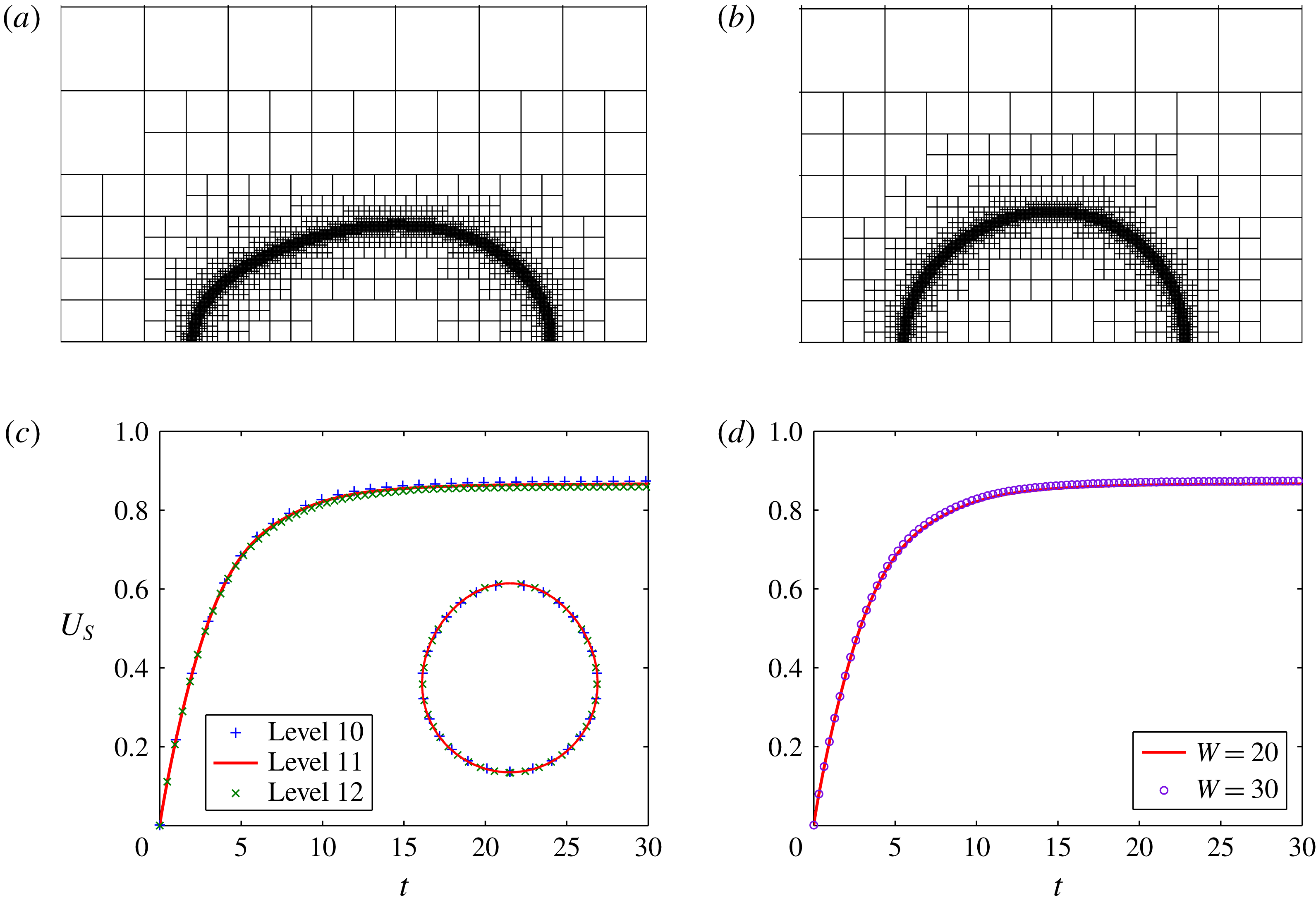
Adaptive grid set-up (a) at
 $t=3.5$
and (b) at
 $t=25$
. (c) Transient variation of settling speed for different grid sizes. (d) Effect of domain size on transient variation of settling speed. Parameters considered are
 $R=2.5$
,
 $S=1$
,
 $\unicode[STIX]{x1D706}=1$
,
 $Ga=10$
,
 $Ca=0.2$
,
 $M=4$
and
 $Re_{E}=0.01$
. Inset of panel (c) shows the steady drop shape comparison for different grid sizes.

To examine the effect of the electric field, the present numerical results are compared with the numerical results of Lac & Homsy (Reference Lac and Homsy2007). Figure 17 depicts the variation of EHD deformation of a neutrally buoyant LD drop suspended in LD medium with electric capillary number
 $Ca_{E}=a\unicode[STIX]{x1D700}_{e}\overline{E}_{0}^{2}/\unicode[STIX]{x1D6FE}$
for
 $R=10,S=0.1$
and
 $\unicode[STIX]{x1D706}=1$
. Here
 $Ca_{E}$
represents the ratio of electric stress to capillary stress. The deformation obtained by the present numerical simulations agrees very well with the numerical results of Lac & Homsy (Reference Lac and Homsy2007) up to high
 $Ca_{E}$
as seen in figure 17.
Appendix B. Grid and domain independence tests
Grid and domain independence tests are performed using the parameters
 $R=2.5$
,
 $S=1$
,
 $Ga=10$
,
 $Ca=0.2$
,
 $M=4$
and
 $Re_{E}=0.01$
. For the present simulation, the grid levels 11 and 5 are employed in Gerris, which correspond to grid sizes of
 $\unicode[STIX]{x0394}r=W\times 2^{-11}$
and
 $\unicode[STIX]{x0394}r=W\times 2^{-5}$
, respectively. Figures 18(a) and 18(b) illustrate the dynamic adaptive grid structure at times
 $t=3.5$
and
 $t=25$
. To perform the grid independence study, additional simulations have performed keeping grid levels 10 and 12 at the interface and a domain size of
 $H\times W=60\times 20$
. In figure 18(c),
 $U_{S}$
is plotted with
 $t$
for all three grid levels and in the inset a comparison of steady-state drop shapes is provided. Looking into the figure it can be stated that further grid refinement has a negligible effect on drop EHD. Therefore, for the purpose of computational time minimization, the grid level 11 is considered for the simulations. Figure 18(d) displays the transient variation of settling speed for two different domain sizes:
 $W=20$
and
 $W=30$
. The corresponding values of H are 60 and 90, respectively. From figure 18(d), it is evident that even after increasing the domain width by 1.5 times, the drop motion remains unchanged. Hence for the present domain size (
 $H\times W=60\times 20$
), the numerical model achieved domain independence.