





1. Introduction
In classical buoyancy-driven flows such as Rayleigh–Bénard convection, fluid motion is primarily governed by gravity and boundary heating. Warmer, less dense fluid ascends, while cooler, denser fluid descends, which is true for fluids without density anomalies. In many natural and industrial systems, heat is not only externally supplied, but instead produced internally within the system. In planetary interiors, radioactive decay and gravitational compression drive mantle convection, influencing plate tectonics, the geomagnetic field, and the thermal and chemical evolution of planetary interiors (McKenzie et al. Reference McKenzie, Roberts and Weiss1973; Schubert et al. Reference Schubert, Turcotte and Olson2001; Samuel & Farnetani Reference Samuel and Farnetani2003; Ricard Reference Ricard2007; Nakagawa & Tackley Reference Nakagawa and Tackley2014). Internal heating (IH) also governs atmospheric convection on Venus (Tritton Reference Tritton1975) and the formation of polygonal terrain on Pluto (Trowbridge et al. Reference Turnbull2016). An IH fluid can therefore cause buoyancy-driven flows even without boundary heating in the presence of a volumetric body force such as gravity, which can lead to complex flow patterns and instabilities (see Vilella et al. Reference Wang, Lohse and Shishkina2018).
The dynamics of IH convection is governed by the volumetric heating rate
 $H$
, and characterised by the Rayleigh–Roberts number
 $R$
, derived under the Boussinesq (Reference Boussinesq1903) approximation. In other words, for fluid layers, the Rayleigh number
 $Ra$
is modified by the IH sources, which is related to the temperature difference
 $\Delta T$
(Roberts Reference Roberts1967; Schubert et al. Reference Schubert, Turcotte and Olson2001), leading to the definition
 \begin{equation} R = \frac {\alpha \Delta \textit{Tg} d^3}{\nu \kappa }, \quad \text{with} \quad \Delta T = \frac {Hd^2}{k}, \end{equation}
where
 $\alpha$
is the thermal expansion coefficient,
 $g$
is the gravitational acceleration,
 $d$
is the layer thickness,
 $\nu$
is the kinematic viscosity,
 $\kappa$
is the thermal diffusivity, and
 $k$
is the thermal conductivity. (The characteristic fluid layer thickness depends on the imposed thermal boundary conditions. For configurations with heating applied only at one boundary, the characteristic length scale is the full layer thickness
 $d$
. In contrast, when both opposite bounding plates are cooled, the appropriate characteristic length scale is
 $d/2$
; Kulacki & Goldstein Reference Kulacki and Goldstein1972; Vilella et al. Reference Wang, Lohse and Shishkina2018.)
Internally heated convection has been sparsely studied in two main configurations. In the first, IH1, the fluid is uniformly heated with both opposite bounding plates at equally fixed temperatures, explored experimentally by Fiedler & Wille (Reference Fiedler and Wille1970), Kulacki & Goldstein (Reference Kulacki and Goldstein1972), Kulacki & Nagle (Reference Kulacki and Nagle1975), Kulacki & Emara (Reference Kulacki and Emara1977) and Lee et al. (Reference Lee, Lee and Suh2007), and via two-dimensional (2-D) and three-dimensional (3-D) direct numerical simulations (DNS) by McKenzie et al. (Reference McKenzie, Roberts and Weiss1973), Emara & Kulacki (Reference Emara and Kulacki1980), Goluskin & Spiegel (Reference Goluskin and Spiegel2012), Goluskin & van der Poel (Reference Goluskin and van der Poel2016), Kazemi et al. (Reference Kazemi, Ostilla-Mónico and Goluskin2022), Arslan et al. (Reference Arslan, Fantuzzi, Craske and Wynn2023) and Arslan & Rojas (Reference Arslan and Rojas2025). In the second configuration, IH2, the bottom boundary is insulated, which was studied experimentally by Lee et al. (Reference Lee, Lee and Suh2007), in 2-D DNS by Peckover & Hutchinson (Reference Peckover and Hutchinson1974), Straus (Reference Straus1976) and Arslan et al. (Reference Arslan, Fantuzzi, Craske and Wynn2023), and in 3-D DNS by Wörner et al. (Reference Yavorskaya, Fomina and Belyaev1997) and Vilella et al. (Reference Wang, Lohse and Shishkina2018). Rotation in the plane layer has also received recent attention, with analytical bounds (Arslan Reference Arslan2024) and 3-D DNS (Ostilla-Mónico & Arslan Reference Ostilla-Mónico and Arslan2025).
A common relationship to characterise convection in IH fluids is the volume-averaged temperature
 $T_{vol}$
, also commonly known as the mean temperature, in contrast to the Rayleigh–Roberts number and the Prandtl number. So far, experiments and DNS have shown a decrease of
 $T_{vol}$
with increasing
 $R$
(Kulacki & Goldstein Reference Kulacki and Goldstein1972; Goluskin & Spiegel Reference Goluskin and Spiegel2012; Goluskin & van der Poel Reference Goluskin and van der Poel2016). Wang et al. (Reference Wörner, Schmidt and Grötzbach2021) provided a scaling
 $T_{vol} \sim R^{-1/5}$
for boundary-layer-dominated regimes, which is consistent with DNS provided by Kazemi et al. (Reference Kazemi, Ostilla-Mónico and Goluskin2022). For larger Prandtl number or turbulent regimes, a scaling
 $T_{vol} \sim R^{-1/4}$
is predicted. Rigorous upper bounds on heat transport in IH convection have further been established using variational methods (Arslan et al. Reference Arslan, Fantuzzi, Craske and Wynn2021a
,
Reference Arslan, Fantuzzi, Craske and Wynnb
; Kumar et al. Reference Kumar, Arslan, Fantuzzi, Craske and Wynn2022).
In microgravity, as considered in the present study, natural convection is absent. As a result, the flow can only be driven by body force densities other than gravity, such as those generated by electric or magnetic fields to which the fluid responds. The asymmetry between the bounding plates characterising classical IH1 convection therefore vanishes, and heat is transported symmetrically between the two boundaries. The relevant questions therefore concern how the boundary layer (BL) thickness and
 $T_{vol}$
vary with the Rayleigh–Roberts number and Prandtl number in these systems as a function of the forcing strength.
1.1. Dielectrophoretic convection
Since the pioneering work of Senftleben (Reference Senftleben1932), it has been recognised that electric fields can influence heat transfer in dielectric fluids (Senftleben & Pietzner Reference Senftleben and Pietzner1933; Senftleben & Braun Reference Senftleben and Braun1936). When a polar dielectric fluid is subjected to a high-frequency alternating electric field, permanent molecular dipoles undergo field-driven reorientation. Because this orientational polarisation exhibits a finite relaxation time, the polarisation cannot follow the oscillating field instantaneously, giving rise to a phase lag between the electric field and polarisation. The associated dielectric losses convert electromagnetic energy into volumetric heat, and distribute thermal energy internally. The resulting temperature gradients modify the fluid’s electric permittivity, giving rise to an electrohydrodynamic (EHD) body force, which drives convection even in the absence of gravity. This provides a controllable analogue of classical IH convection by utilising dielectric fluids in a microgravity environment. The EHD force density acting on a dielectric fluid is given by
 \begin{equation} \boldsymbol{f}_{\!\textit{EHD}} = \rho _e \boldsymbol{E} - \frac {1}{2} \boldsymbol{E}^2\, \boldsymbol{\nabla } \epsilon + \boldsymbol{\nabla } \left [ \rho \left (\frac {\partial \epsilon }{\partial \rho }\right )_T \frac {\boldsymbol{E}^2}{2} \right ]\!, \end{equation}
where
 $\rho _e$
is the density of free electric charge,
 $\boldsymbol{E}$
is the electric field,
 $\rho$
is the fluid density,
 $\epsilon$
is the electric permittivity, and
 $T$
is the temperature (Landau et al. Reference Landau, Lifshits and Pitaevskiĭ1984). The three terms on the right-hand side represent the electrophoretic (Coulomb), dielectrophoretic (DEP) and electrostrictive force densities, respectively. At small frequencies, the Coulomb force density on free charges dominates the flow dynamics, even in initially electroneutral media. To ensure that charge-related effects remain negligible, the field frequency must satisfy
 \begin{equation} \omega \gg \tau _e^{-1}, \tau _\nu ^{-1}, \tau _\kappa ^{-1}, \tau _m^{-1}, \tau _d^{-1}, \end{equation}
where
 $\omega$
is the angular frequency of the applied alternating electric field. This high-frequency condition states, with the characteristic time scales of charge relaxation
 $\tau _e$
, viscous dissipation
 $\tau _\nu$
, thermal diffusion
 $\tau _\kappa$
, ion migration
 $\tau _m$
and mass diffusion
 $\tau _d$
, that a dielectric fluid is unable to respond dynamically, and the resulting Coulomb force density cancels out over a period of the electric field variation. The remaining forces are the DEP force density and the electrostrictive force density, as both have non-zero time average because of
 $\boldsymbol{E}^2$
and the time-averaged dielectric heating rate
 $H$
(see Yoshikawa et al. Reference Zaussinger, Haun, Szabo, Travnikov, Al Kawwas and Egbers2020). In the absence of mobile boundaries, the electrostrictive force has no effect on the motion of an incompressible fluid, which is considered for the particular working fluid (see Turnbull Reference Turnbull1968; Jones Reference Jones1979; Yoshikawa et al. Reference Zaussinger, Krebs, Travnikov and Egbers2013b
). The remaining force is due to the DEP force density, which depends on the temperature-sensitive permittivity
 $\epsilon (T)$
, and varies among dielectric fluids. In most cases, it decreases with increasing temperature. For the majority of fluids,
 $\epsilon (T)$
can be approximated by the equation of state written as
 \begin{equation} \epsilon (T) = \epsilon _0 \epsilon _{{r}} \left [1 - e \left (T - T_0\right )\right ]\!, \end{equation}
where
 $\epsilon _0 = 8.854 \times 10^{-12}$
F m
 $^{-1}$
is the vacuum permittivity,
 $\epsilon _{{r}}$
is the relative permittivity,
 $e = -(1/\epsilon _{{r}})\,\partial \epsilon _{{r}}/\partial T$
is the thermal permittivity coefficient (typically
 $10^{-3}$
–
 $10^{-1}$
K
 $^{-1}$
), and
 $T_0$
is the reference temperature where the fluid parameters are defined (see Yoshikawa et al. Reference Zaussinger, Krebs, Travnikov and Egbers2013b
; Mutabazi et al. Reference Mutabazi, Yoshikawa, Fogaing, Travnikov, Crumeyrolle, Futterer and Egbers2016; Szabo & Egbers Reference Szabo and Egbers2025).
To isolate the DEP force density from Archimedean buoyancy, many experiments are conducted under microgravity. The arising convective phenomenon is known as thermoelectrohydrodynamic (TEHD) convection. This particular kind of convection in an incompressible dielectric fluid has been studied in planar fluid layers (see Turnbull Reference Turnbull1968; Roberts Reference Roberts1969; Takashima Reference Takashima1976; Stiles Reference Stiles1991; Yoshikawa et al. Reference Yoshikawa, Kang, Mutabazi, Zaussinger, Haun and Egbers2013b ; Barry et al. Reference Barry, Kang, Yoshikawa and Mutabazi2023) and cylindrical annuli (see Takashima Reference Takashima1980; Yavorskaya et al. Reference Yoshikawa, Crumeyrolle and Mutabazi1984; Yoshikawa et al. Reference Yoshikawa, Tadie Fogaing, Crumeyrolle and Mutabazi2013a ; Travnikov et al. Reference Travnikov, Crumeyrolle and Mutabazi2015, Reference Travnikov, Crumeyrolle and Mutabazi2016; Meier et al. Reference Meier, Jongmanns, Meyer, Seelig, Egbers and Mutabazi2018; Szabo et al. Reference Szabo, Meier, Meyer, Barry, Motuz, Mutabazi and Egbers2021, Reference Szabo, Meyer, Meier, Motuz, Sliavin and Egbers2022, Reference Szabo, Gaillard, Zaussinger and Egbers2023; Kang et al. Reference Kang, Mutabazi and Yoshikawa2024), which are more relevant to heat transfer enhancement considering applications such as in a heat exchanger. The influence of the DEP force density has also been investigated in spherical geometries, primarily to model large-scale geophysical flows (see Chandra & Smylie Reference Chandra and Smylie1972; Hart et al. Reference Hart, Glatzmaier and Toomre1986; Beltrame et al. Reference Beltrame, Egbers and Hollerbach2003; Egbers et al. Reference Egbers, Beyer, Bonhage, Hollerbach and Beltrame2003; Travnikov et al. Reference Travnikov, Szabo, Gaillard and Egbers2003; Zaussinger et al. Reference Zaussinger, Haun, Szabo, Travnikov, Al Kawwas and Egbers2020; Travnikov & Egbers Reference Travnikov and Egbers2021). A pioneering geophysical experiment proposed by Chandra & Smylie (Reference Chandra and Smylie1972) and later realised by Hart et al. (Reference Hart, Glatzmaier and Toomre1986) evolved into the GeoFlow series aboard the International Space Station (see Beltrame et al. Reference Beltrame, Egbers and Hollerbach2003; Egbers et al. Reference Egbers, Beyer, Bonhage, Hollerbach and Beltrame2003; Travnikov et al. Reference Travnikov, Szabo, Gaillard and Egbers2003; Zaussinger et al. Reference Zaussinger, Haun, Szabo, Travnikov, Al Kawwas and Egbers2020; Travnikov & Egbers Reference Travnikov and Egbers2021), where a central force field in a spherical shell simulated mantle–core flow. The flow dynamics, visualised via Wollaston shearing interferometry, was validated against numerical models (see Futterer et al. Reference Futterer, Egbers, Dahley, Koch and Jehring2010, Reference Futterer, Krebs, Plesa, Zaussinger, Hollerbach, Breuer and Egbers2013; Zaussinger et al. Reference Zaussinger, Krebs, Travnikov and Egbers2017). A follow-up experiment, AtmoFlow, is currently in preparation (see Travnikov & Egbers Reference Travnikov and Egbers2021; Gaillard et al. Reference Gaillard, Szabo and Egbers2024, Reference Gaillard, Szabo, Travnikov and Egbers2025; Travnikov et al. Reference Travnikov, Zaussinger, Haun and Egbers2025; Gaillard et al. Reference Gaillard, Szabo, Travnikov and Egbers2026), which aims to investigate planetary atmospheres. For a broader discussion of TEHD convection, the reader is referred to the review by Mutabazi et al. (Reference Mutabazi, Yoshikawa, Fogaing, Travnikov, Crumeyrolle, Futterer and Egbers2016), which provides a detailed overview of the onset of TEHD convection in different geometries, and discusses the electric Rayleigh number, a key non-dimensional parameter originally introduced by Turnbull (Reference Turnbull1968) and Roberts (Reference Roberts1969).
1.2. Convection in internally dielectric heated fluids
Most prior studies have focused on perfect dielectric fluids and neglected dielectric losses, thereby excluding IH terms from the energy equation. Only a few experiments involving polar fluids in spherical geometries have considered these losses explicitly (see Travnikov et al. Reference Tritton2020; Zaussinger et al. Reference Zaussinger, Haun, Szabo, Travnikov, Al Kawwas and Egbers2020; Travnikov & Egbers Reference Travnikov and Egbers2021). A recent study by Yoshikawa et al. (Reference Zaussinger, Haun, Szabo, Travnikov, Al Kawwas and Egbers2020) investigated TEHD convection in a plane capacitor under microgravity and terrestrial conditions, using a dielectric fluid heated via dielectric loss between bounding plates. In this context, the electric Rayleigh number was reformulated to account for electric field effects and dielectric heating, yielding a form analogous to the Rayleigh–Roberts number introduced in (1.1). A crucial parameter for the study was the thermoelectric coupling parameter
 $\gamma _e$
, which accounts for electric field variations in Gauss’s law related to the temperature-dependent electric permittivity defined in (1.4). This parameter is dependent on the used dielectric fluid and the caused dielectric losses that induce temperature gradients throughout the fluid (see Yoshikawa et al. Reference Yoshikawa, Kang, Mutabazi, Zaussinger, Haun and Egbers2013b
). For the onset of convection,
 $\gamma _e$
is relevant; however, it increases with
 $\Delta T$
for values above the onset.
1.3. Aim and objectives
The present work investigates TEHD convection in internal dielectric heated polar fluids, extending the parameter space of the numerical simulations by Yoshikawa et al. (Reference Zaussinger, Haun, Szabo, Travnikov, Al Kawwas and Egbers2020) using an alcohol-based fluid (1-Nonanol) and a fluorinated based fluid (Novec 7200), with fluid properties listed in table 2 in Appendix A. We investigate the flow structures and dynamics of a fluid layer subjected to internal dielectric heating and cooled from opposite bounding plates, defined earlier as IH1, in the absence of gravity, following the configuration of Yoshikawa et al. (Reference Zaussinger, Haun, Szabo, Travnikov, Al Kawwas and Egbers2020). Using DNS, we compare the resulting behaviour with that of conventionally IH fluids, such as those studied by Goluskin (Reference Goluskin2016) and Vilella et al. (Reference Wang, Lohse and Shishkina2018).
2. Model formulation
2.1. Problem geometry
The system investigated consists of a dielectric fluid layer of height
 $d$
, laterally with periodic conditions, subjected to constant uniform temperature of the bounding plates in space and time. The length and width of the fluid layer are equal, and are a multiple of four times the extracted wavelength found in Yoshikawa et al. (Reference Zaussinger, Haun, Szabo, Travnikov, Al Kawwas and Egbers2020). No-slip velocity conditions are imposed at both bounding plates. An alternating electric tension
 $V(t)$
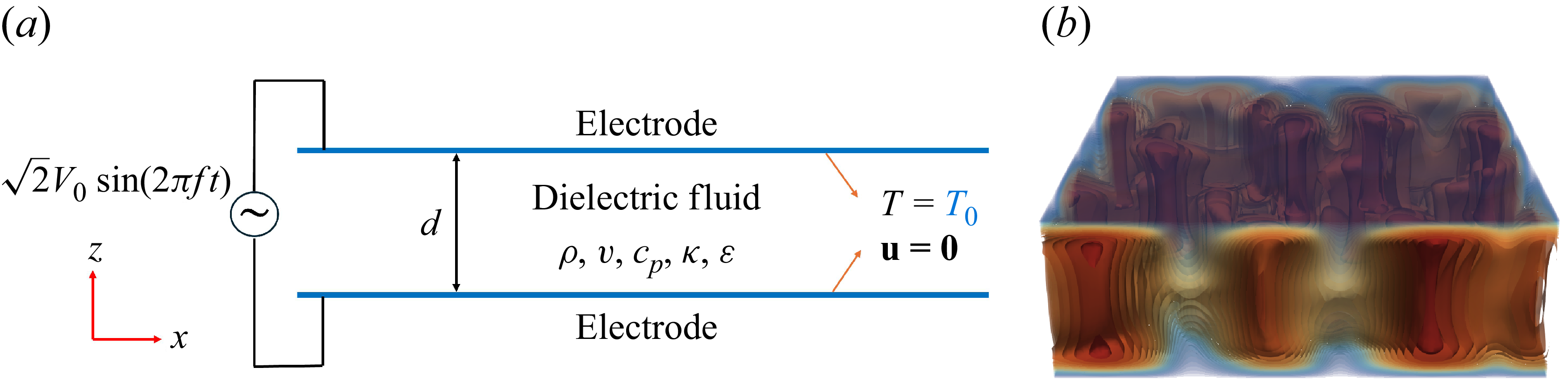
is applied between the bounding plates, whereas one of the bounding plate is grounded. The influence of the resulting electric field on fluid flow and heat transfer is investigated by varying the applied electric tension causing the fluid to heat and investigating two different dielectric loss factors that have been measured for both fluids for an alternating frequency of 50 Hz and 10 kHz. A schematic of the configuration is shown in figure 1.
(a) Schematic of the problem geometry. (b) A representative 3-D temperature field of the numerical data presented in figure 2(d).
2.2. Governing equations
The high-frequency condition in (1.3) ensures that the fluid remains initially electroneutral, preventing space charge accumulation (
 $\rho _e = 0$
) throughout the development of the convective flow. When the condition
 $d \gg \lambda _D$
is satisfied, where
 $\lambda _D$
is the Debye length, the convective transport of charge from the diffuse layer into the bulk is negligible (see Yoshikawa et al. Reference Zaussinger, Krebs, Travnikov and Egbers2013b
). Under these assumptions, the fluid motion in a dielectric layer can be described using the continuity, momentum and energy equations together with Gauss’s law and the EHD Boussinesq approximation, given in (1.4) and read as
 \begin{equation} \boldsymbol {\nabla }\boldsymbol{\cdot }\boldsymbol{u} = 0, \end{equation}
 \begin{equation} \partial _t \boldsymbol{u} + (\boldsymbol{u} \boldsymbol{\cdot } \boldsymbol{\nabla }) \boldsymbol{u} = -\frac {1}{\rho } \boldsymbol{\nabla }\!P + \nu \,{\nabla} ^2 \boldsymbol{u} + \frac {1}{\rho } \boldsymbol{f}_{\!\textit{DEP}}, \end{equation}
 \begin{equation} \partial _t T + (\boldsymbol{u} \boldsymbol{\cdot } \boldsymbol{\nabla }) T = \kappa\, {\nabla} ^2 T + H, \end{equation}
 \begin{equation} \boldsymbol {\nabla }\boldsymbol{\cdot }\left [\epsilon (T)\, \boldsymbol{E}\right ] = 0, \quad \text{with} \quad \boldsymbol{E} = -\boldsymbol{\nabla }\phi, \end{equation}
where
 $\boldsymbol{u}$
is the velocity field,
 $\phi$
is the electric potential, and
 $\boldsymbol{f}_{\!\textit{DEP}}$
is the DEP force density. The generalised EHD Boussinesq approximation states that all thermophysical properties are kept constant except for the electrical permittivity in Gauss’s law and in the DEP force density term. This exception is necessary because gradients of electrical permittivity constitute the leading-order mechanism responsible for electrothermal forcing. In the present configuration, the electric-field inhomogeneity is not imposed geometrically, e.g. by curvature, but arises from temperature-induced variations of the electrical permittivity, which generate spatial variations of the electric field and consequently the DEP forcing (see Yoshikawa et al. Reference Zaussinger, Haun, Szabo, Travnikov, Al Kawwas and Egbers2020). The modified pressure
 $P$
is defined by
 \begin{equation} P = p - \frac {1}{2} \rho \left ( \frac {\partial \epsilon }{\partial \rho } \right )_T \boldsymbol{E}^2, \end{equation}
which incorporates the electrostrictive contribution, given by the third term in (1.2), which does not influence the fluid motion if the fluid is incompressible and has no mobile boundaries.
Assuming a sinusoidal electric tension
 $V(t) = \sqrt {2}V_0 \sin (2\pi f t)$
, its root mean square value is defined as
 $V_0 = \sqrt {\langle V^2(t) \rangle _t}$
, where
 $\langle {\cdot }\rangle _t$
denotes time averaging over one oscillation period. The time-averaged DEP approximation can be traced back to a parametric study on the validity of TEHD convection, where the condition
 $2\pi f \tau _\nu \gtrsim 100$
was identified as a key criterion (Smorodin & Velarde Reference Smorodin and Velarde2001; Yoshikawa et al. Reference Zaussinger, Haun, Szabo, Travnikov, Al Kawwas and Egbers2020). Experiments have been conducted within an electrical frequency range of approximately
 $10^{2}$
–
 $10^{4}$
Hz, thereby satisfying this requirement and ensuring the applicability of the approximation (see Turnbull Reference Vilella, Limare, Jaupart, Farnetani, Fourel and Kaminski1969; Chandra & Smylie Reference Chandra and Smylie1972; Hart et al. Reference Hart, Glatzmaier and Toomre1986; Futterer et al. Reference Futterer, Krebs, Plesa, Zaussinger, Hollerbach, Breuer and Egbers2013; Yoshikawa et al. Reference Zaussinger, Haun, Szabo, Travnikov, Al Kawwas and Egbers2020; Szabo et al. Reference Szabo, Meier, Meyer, Barry, Motuz, Mutabazi and Egbers2021). Consequently, the time-averaged DEP force density, accounting for the temperature dependence of the permittivity (see (1.4)), becomes
 \begin{equation} \boldsymbol{f}_{\!\textit{DEP}} = -\frac {1}{2} \boldsymbol{E}^2\, \boldsymbol{\nabla } \epsilon (T) = \frac {\epsilon _0 \epsilon _{{r}} e}{2} \left | -\boldsymbol{\nabla } \phi \right |^2 \boldsymbol{\nabla } T, \end{equation}
where the electric field is expressed as
 $\boldsymbol{E} = -\boldsymbol{\nabla } \phi$
based on the time-averaged electric potential.
The dielectric loss of the working fluid is given by the loss factor and calculated from the ratio between the dissipative and reactive components of the complex electrical permittivity, written as
 \begin{equation} \text{loss factor} \equiv \tan \delta = \frac {\omega \epsilon '' + \sigma }{\omega \epsilon '}, \end{equation}
where
 $\epsilon '$
and
 $\epsilon ''$
are the real and imaginary parts of the complex electrical permittivity,
 $\epsilon = \epsilon ' - \mathrm{i}\epsilon ''$
, with
 $\mathrm{i}=\sqrt {-1}$
. The parameter
 $\delta$
is the dielectric loss angle, and
 $\sigma$
is the electrical conductivity. The volumetric heating rate for a dielectrically heated fluid,
 $H$
, can be defined by
 \begin{equation} H = \frac {\omega \tan \delta \ \epsilon _0 \epsilon _{{r}} }{\rho c_{\!p}} \boldsymbol{E^2} \end{equation}
and is consistent with Travnikov et al. (Reference Tritton2020), Zaussinger et al. (Reference Zaussinger, Haun, Szabo, Travnikov, Al Kawwas and Egbers2020) and Travnikov & Egbers (Reference Travnikov and Egbers2021). The respective temperature increase related to dielectric heating can be defined by the equilibrium between the heating power and the thermal diffusion, and can be estimated by
 \begin{equation} \Delta T = \frac {\omega \tan \delta \, \epsilon _0\epsilon _{{r}} V_0^2}{8k}, \end{equation}
and its variation in the electrical permittivity by the dimensionless thermoelectric parameter
 $\gamma _e= (\epsilon / (\epsilon _0\epsilon _{{r}} ) )-1$
by
 \begin{equation} \gamma _e=e\Delta T = \frac {\omega \tan \delta \ e\epsilon _0\epsilon _{{r}}\kern-1.5pt V_0^2}{8k}, \end{equation}
which is consistent with the assumption by Yoshikawa et al. (Reference Zaussinger, Haun, Szabo, Travnikov, Al Kawwas and Egbers2020), by considering the half-gap distance
 $d/2$
as the characteristic length scale, as the temperature variation predominantly occurs across this region within the dielectric fluid layer, which is defined as the IH1 configuration.
The governing equations (2.1)–(2.4), including the DEP force density given in (2.6), can be non-dimensionalised using appropriate reference scales. For convection-driven flows, the characteristic thermal time scale
 $d^2/\kappa$
is employed. Introducing the following non-dimensional variables,
 \begin{align} \begin{aligned} &\boldsymbol{u}^* = \boldsymbol{u} \frac {d}{\kappa }, \quad t^*= t \frac {\kappa }{d^2}, \quad {\nabla} ^* = d\, \boldsymbol{\nabla }, \\ &P^* = P \frac {d^2}{\rho \kappa ^2}, \quad T^* = \frac {T-T_0}{\Delta T}, \quad \boldsymbol{E}^*= \boldsymbol{E} \frac {d}{V_0}, \end{aligned} \end{align}
the conservation equations can be expressed in non-dimensional form, without asterisks, by
 \begin{equation} \boldsymbol{\nabla }\boldsymbol{\cdot }\boldsymbol{u} = 0, \end{equation}
 \begin{equation} \begin{aligned} {\textit{Pr}}^{-1} \big [ \partial _{t} \boldsymbol{u} + (\boldsymbol{u} \boldsymbol{\cdot } \boldsymbol{\nabla }) \boldsymbol{u} \big ] &= -{\textit{Pr}}^{-1}\, \boldsymbol{\nabla }\!P + \boldsymbol{\nabla}^{2} \boldsymbol{u} + 2 \,\gamma _e^{-1} R_E \boldsymbol{E}^2 \boldsymbol{\nabla }T, \end{aligned} \end{equation}
 \begin{equation} \partial _{t} T + (\boldsymbol{u} \boldsymbol{\cdot }\boldsymbol{\nabla }) T = \boldsymbol{\nabla}^{2} T + 8 \boldsymbol{E}^2, \end{equation}
 \begin{equation} \boldsymbol {\nabla }\boldsymbol{\cdot }\left [ \left (1 - \gamma _e T \right ) \boldsymbol{E} \right ] = 0, \quad \text{with} \quad \boldsymbol{E} = -\boldsymbol {\nabla }\vartheta, \end{equation}
where
 $\vartheta$
is the non-dimensional electric potential, and
 $\textit{Pr}$
is the Prandtl number given by the dissipation time scale ratio
 $\tau _\kappa /\tau _\nu$
. These conservation equations describe electrothermally driven convection, where fluid motion is forced by temperature-induced variations in the dielectric permittivity rather than by gravity as in Rayleigh–Bénard convection. Temperature fluctuations evolve according to (2.14), modify the electric field via (2.15), and generate the body force
 $2\,\gamma _e^{-1} R_E \,\boldsymbol{E}^2\, \boldsymbol{\nabla }T$
that drives the momentum equation (2.13).
To account for electric forcing, the Rayleigh–Roberts number is reformulated by replacing the temperature difference and gravity in (1.1) with (2.9) and the electric gravity, which reads
 $g_{e,0}=2e\epsilon _{{r}}\epsilon _0\gamma _eV_0^2/(\rho \alpha d^3)$
, respectively (see Yoshikawa et al. Reference Zaussinger, Haun, Szabo, Travnikov, Al Kawwas and Egbers2020). This results in an electric Rayleigh–Roberts number given by
 \begin{equation} R_E = \frac {\alpha \Delta \textit{Tg}_{e,0}}{\nu \kappa } \left ( \frac {d}{2} \right )^3 = \frac {(\omega \tan \delta )^2 e^2 (\epsilon _0 \epsilon _{{r}})^3 V_0^6}{256 \rho \nu \kappa k^2} = \frac {1}{4} \gamma _e^2 V_{E}^2, \end{equation}
where
 \begin{equation} V_{E} = V_0 / \sqrt {\rho \nu \kappa / (\epsilon _0 \epsilon _{{r}})} \end{equation}
is the non-dimensional effective electric potential. Note that
 $V_{E}$
depends on fluid properties and can vary significantly between different dielectric liquids such as hydrofluoroethers and alcohols (see Szabo & Egbers Reference Szabo and Egbers2025).
3. Computational methodology
3.1. Numerical input, schemes and solvers
The governing equations are solved using a finite-volume formulation implemented in the open-source software package OpenFOAM v2012. The problem geometry shown in figure 1 is subjected to the boundary conditions
 \begin{equation} \left \{ \begin{array}{ll} \boldsymbol{u}=\boldsymbol{0},\ T=0,\ \vartheta =1 & \text{at } \quad z=1, \\[5pt] \boldsymbol{u}=\boldsymbol{0},\ T=0,\ \vartheta =0 & \text{at } \quad z=0, \end{array} \right . \end{equation}
and solved via a custom-developed buoyantPimpleFoam solver developed by (Gaillard et al. Reference Gaillard, Szabo and Egbers2024, Reference Gaillard, Szabo, Travnikov and Egbers2025). The numerical solution proceeds in two stages: first, the electrostatic and thermal base state is obtained by solving Gauss’s law and the energy equation. This solution is then used to initialise the fully coupled, time-dependent simulation of the electric, thermal and flow fields. Further details regarding spatial and temporal discretisation, linear solvers and algorithmic implementation are provided in Appendix B.
3.2. Parameter choice
Two dielectric fluids, 1-Nonanol and Novec 7200, are selected due to their contrasting dielectric loss factors, which result in significantly different volumetric heating rates. These fluids also differ in Prandtl number, and have previously been used to study heat transfer enhancement by Yoshikawa et al. (Reference Zaussinger, Haun, Szabo, Travnikov, Al Kawwas and Egbers2020), and in modelling geophysical and astrophysical flows at laboratory scale (see Zaussinger et al. Reference Zaussinger, Haun, Szabo, Travnikov, Al Kawwas and Egbers2020; Travnikov & Egbers Reference Travnikov, Egbers and Hollerbach2021).
The volumetric heating rate
 $H$
depends on the dielectric loss factor
 $\tan \delta$
, angular frequency
 $\omega$
, and applied electric tension
 $V$
. We experimentally measured
 $\tan \delta$
at two frequencies, and varied
 $V$
to define a parameter space suitable for physical experiments, such as those in planar cavities studied by Strangfeld et al. (Reference Strangfeld, Bölük, Szabo, Meier, Meyer, Sliavin, Motuz and Egbers2022) and Szabo & Egbers (Reference Szabo and Egbers2025). To facilitate comparisons with numerical simulations and experiments involving additional gravitational forcing, we use the dimensionless effective electric potential
 $V_{E}$
instead of the electric Rayleigh–Roberts number. This choice avoids coupling complications between an arbitrarily selected electric Rayleigh–Roberts number and the Rayleigh number given e.g. in equations (20) and (21) in Yoshikawa et al. (Reference Zaussinger, Haun, Szabo, Travnikov, Al Kawwas and Egbers2020). This ensures reproducibility in both simulations and experiments by directly mapping
 $V_{ E}$
to a unique fluid and heating condition.
The parameter space is based on a prior conducted 2-D numerical parametric sweep to investigate the nature of the flow and the evolving convective patterns. For the 3-D numerical simulations, the values of
 $V_{E}$
could then be chosen and ranged for 1-Nonanol from 1400 to 3000, while for Novec 7200 the range was 6000–11 000. Simulations were carried out with the two frequencies 50 Hz and 10 kHz, where fluid parameters are known by physical measurements. Using the fluid properties and measured loss factors listed in table 2, the corresponding forcing parameters were calculated (see table 1), which define the parameter space explored in the present study. To get an indication of the parameter space in relation to
 $\gamma _e$
,
 $R_E$
and
 $V_{E}$
, the relationships between their individual strengths can be plotted using (2.10), (2.16) and (2.17), respectively.
Overview of the parameter choice for both working fluids, 1-Nonanol and Novec 7200, at 50 Hz and 10 kHz.
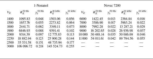
Table 1. Long description
A table comparing properties of Novec 7200 and 1-Nonanol. The table has 16 rows and 5 columns. The columns are labeled Property, Symbol, Novec 7200, 1-Nonanol, and Units. Row 1: Property, Symbol, Novec 7200, 1-Nonanol, Units. Row 2: Kinematic viscosity, v, 0.471, 13.970, 10^-6 m^2 s^-1. Row 3: Density, rho, 1420.000, 828.160, kg m^-3. Row 4: Thermal expansion coeff., alpha, 1.605, 0.823, 10^-3 K^-1. Row 5: Thermal permittivity coeff., e, 2.407, 10.209, 10^-3 K^-1. Row 6: Electric permittivity (relative), epsilon_r, 7.393, 9.056, -. Row 7: Dielectric loss factor (50 Hz), tan delta, 8.570, 10.660, -. Row 8: Dielectric loss factor (10 kHz), tan delta, 5.525, 6.242, 10^-2. Row 9: Thermal diffusivity, kappa, 4.510, 7.940, 10^-8 m^2 s^-1. Row 10: Thermal conductivity, k, 0.070, 0.163, W K^-1 m^-1. Row 11: Reference temperature, T_0, 298.000, 293.000, K. Row 12: Heat capacity, c_p, 1092.000, 2474.000, J kg^-1 K^-1. Row 13: Thermal dissipation time scale, tau_x, 53.100, 1.790, s. Row 14: Viscous dissipation time scale, tau_v, 553.840, 314.861, s. Row 15: Charge relaxation time scale, tau_e, 3.716, 2.988, s. Row 16: Characteristic length, d, 5.000, 5.000, 10^-3 m. Row 17: Prandtl number, Pr, 10.430, 175.945, -.
Fluid properties of Novec 7200 and 1-Nonanol.
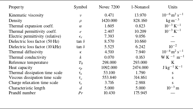
Table 2. Long description
The table compares fluid properties of Novec 7200 and 1-Nonanol. It has two main sections, one for each fluid, with columns for different properties measured at various frequencies. Each section includes columns for V_E, R_E at 50 Hz, gamma sub e at 50 Hz, R_E at 10 kHz, and gamma sub e at 10 kHz. The table lists specific values for these properties at different V_E levels. For 1-Nonanol, the V_E values range from 1400 to 3000, and for Novec 7200, they range from 1422.45 to 11000. Each row provides detailed measurements for the respective fluid at the given V_E level.
3.3. Diagnostics
To assess the influence of the chosen parameter space on convective and thermal transport, we introduce several diagnostic measures. Volume-averaged quantities are denoted by angle brackets
 $\langle {\cdot }\rangle _V$
, and overbars
 $\overline {\vphantom{0}\ldots }$
indicate temporal averages. The intensity of convection is characterised by the dimensionless kinetic energy density
 $\tilde {E}_{K}$
, which reflects the strength of advective heat transport over time. The corresponding non-dimensional volume-averaged temperature
 $T_{vol}$
provides an indication of how well heat is diffused in the overall fluid layer. These quantities are defined as
 \begin{equation} \tilde {E}_K = \frac {1}{2}\, \overline {\langle |\boldsymbol{u}|^2 \rangle _V}, \quad T_{vol} = \langle \overline {T} \rangle _V, \end{equation}
where spatial averaging is performed first, followed by temporal averaging across the entire domain after the flow has equilibrated from the initial state for
 $\tilde {E}_{K}$
, and vice versa for
 $T_{vol}$
.
The overall heat transfer enhancement is characterised by the Nusselt number. We consider the IH1 formulation by Goluskin (Reference Goluskin2016) given by
 \begin{equation} \textit{Nu}_H=\frac {q_w}{T_{\textit{max}} - T_w} \frac {d}{4k} = \frac {\,\bigr | \partial T / \partial z \bigr |_{\substack {w}}}{T_{\textit{max}} - T_w}\frac {d}{4}, \end{equation}
where
 $q_w$
is the conductive flux through one of the boundary plates, with
 $T_{\textit{max}}-T_w$
defined as the maximum temperature difference measured across the fluid layer. A value
 $\textit{Nu}_{H} = 1$
represents pure conduction, and
 $\textit{Nu}_{H} \gt 1$
reflects convective heat transfer in IH1 fluids (Kulacki & Goldstein Reference Kulacki and Goldstein1972; Goluskin Reference Goluskin2016).
In laboratory settings where gravity is present, Archimedean buoyancy can drive convection in non-isothermal fluids, thereby modifying the energy transport within the system. As a result, heat may be dissipated unevenly between both bounding plates; see e.g. figure 2 in Kulacki & Goldstein (Reference Kulacki and Goldstein1972). In this study, as indicated by the conservation equation, we examine the IH1 configuration in the absence of gravity.
3.4. Validation and numerical resolution
The solver has been extensively validated in previous studies for both natural and TEHD convection, showing deviations of less than 1 % relative to pseudo-spectral and finite-element benchmarks (Gaillard et al. Reference Gaillard, Szabo and Egbers2024, Reference Gaillard, Szabo, Travnikov and Egbers2025). For the present fluid-layer configuration, additional benchmark comparisons are performed against the reference solutions of Barry et al. (Reference Barry, Kang, Yoshikawa and Mutabazi2023). Excellent agreement is obtained across the full parameter range, including at high Rayleigh numbers, with discrepancies remaining below 1 % (see figure 10(a) below). Mesh-independence tests confirm that all results reported here are numerically converged. Further details of the benchmark configuration and grid-resolution study are provided in Appendix C.
4. Results
This section presents the observed convective structures, which are characterised by their convective morphology. We analyse temperature and velocity profiles, and relate the imposed thermal forcing to the thermal and kinetic BL thicknesses, and energy dissipation in the BL and the bulk of the fluid. The kinetic energy and volume-averaged temperature are discussed, together with the heat transfer quantified by the Nusselt number with respect to the applied forcing.
4.1. Visualisation and characterisation of observed convective morphology
Iso-surfaces of the non-dimensional temperature
 $T$
projected along the
 $x$
,
 $y$
and
 $z$
directions of 1-Nonanol at 50 Hz: (a)
 $V_E=1500$
(
 $R_E = 1657$
), (b)
 $V_E=1600$
(
 $R_E = 2441$
), (c)
 $V_E=1900$
(
 $R_E = 6846$
), (d)
 $V_E=3000$
(
 $R_E = 106\,096$
).
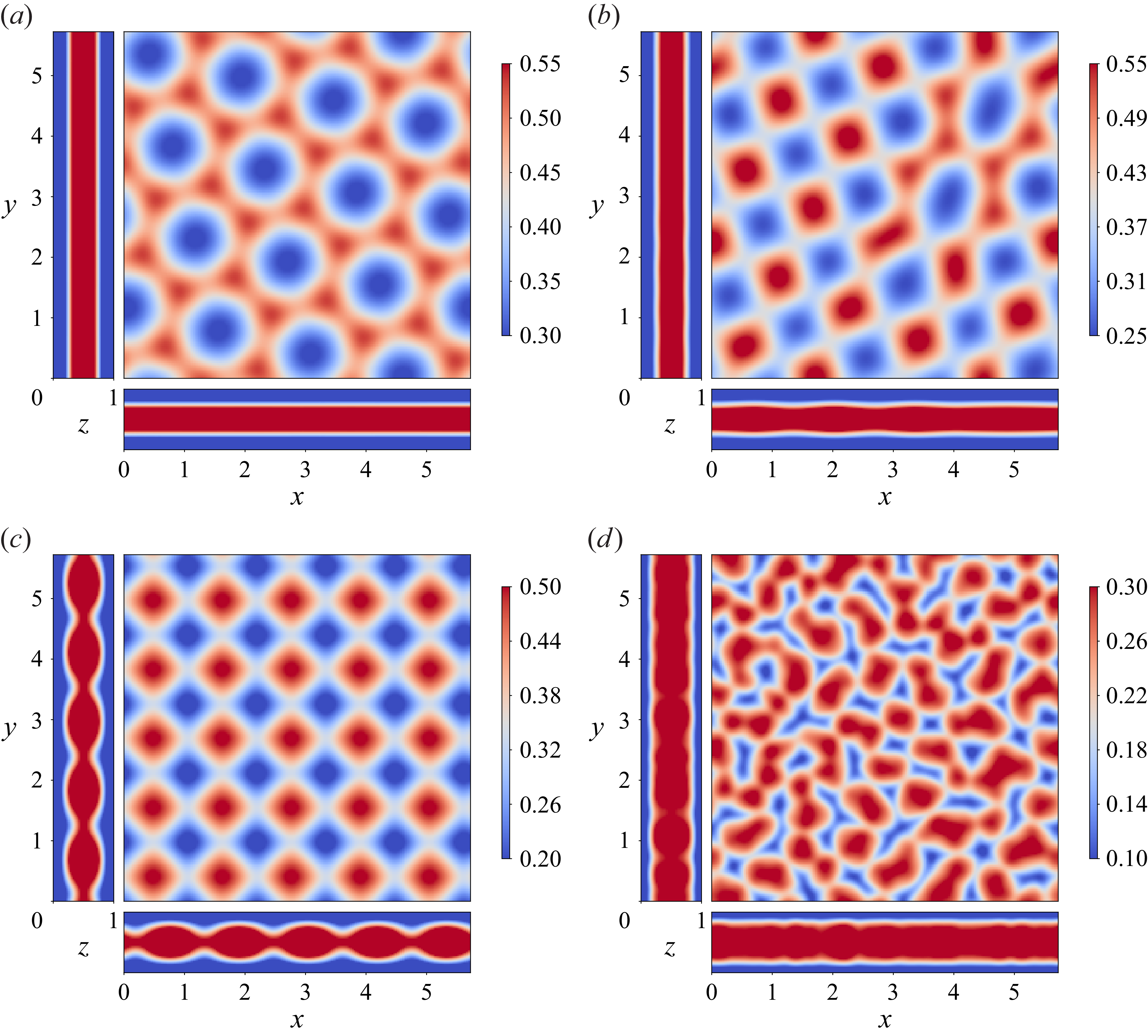
The characterisation of convective patterns is based on the temporal evolution and spatial organisation of flow structures. Figure 2 shows iso-surface snapshots of the temperature field
 $T$
projected along the
 $x$
,
 $y$
and
 $z$
directions, after the system has reached a stationary or quasi-stationary state. The simulations reveal time-invariant plumes shown in figures 2(a–c), and time-dependent convection depicted in figure 2(d). Four distinct regimes can be classified: at small effective voltage
 $V_{E}=1500$
, the plumes form hexagonal patterns evident in the
 $z$
projection, as seen in figure 2(a), but are obscured in the
 $x$
and
 $y$
directions due to their oblique orientation. Increasing
 $V_{E}$
to 1600 as shown in figure 2(b) results in a mixed state of hexagonal and rectangular patterns, with a higher plume density. The section-averaged fields indicate emerging structures in the
 $y$
direction, while the
 $x$
direction remains patternless due to obliqueness. With an additional increase to
 $V_{E}=2500$
given in figure 2(c), plumes align along the
 $x$
and
 $y$
axes, forming well-defined rectangular patterns visible in all projections. At
 $V_{E}=3000$
, shown in figure 2(d), the flow becomes time-dependent, indicative of deep convection.
4.2. Mean temperature and velocity profiles
To obtain temporally and spatially averaged temperature and velocity profiles, we first perform a temporal average for each grid point, followed by sectional averaging in the
 $x$
direction and then in the
 $y$
direction over the entire fluid layer. The resulting profiles, denoted as
 $\langle \overline {T}\rangle _S(z)$
for temperature, and
 $\langle \overline {U}\rangle _S(z)$
for velocity magnitude denoted by
 $U = |\boldsymbol{u}|$
, characterise the mean behaviour throughout the fluid bulk. The overbar
 $\overline {\vphantom{0}\ldots }$
represents temporal averaging, and
 $\langle {\cdot }\rangle _S$
denotes spatial averaging over the respective cross-sectional plane
 $S$
, which is consistent with the notation introduced in the diagnostics subsection (§ 3.3). Figure 3 depicts representative profiles of temperature and velocity between the bounding plates for selected values of effective voltage
 $V_E$
, spanning the explored range of both working fluids and dielectric loss factors.
In all cases, the temperature profile, given in figures 3(a–d), rises from one bounding plate to mid-depth (
 $z = d/2$
), then decreases towards the other bounding plate, indicating internal dielectric heating with heat dissipated symmetrically towards both cooled boundaries. For small
 $V_E$
, the profile is approximately parabolic and extends throughout the bulk, reflecting a thick thermal BL. As
 $V_E$
increases, the profile flattens near the centre and steepens near the boundaries, indicating the development of thinner thermal BLs. While the profiles remain symmetric, they deviate from the parabolic shape observed at low
 $V_E$
. The steep gradients near the boundaries indicate a reduction in BL thickness, consistent with previous studies (see Parmentier & Sotin Reference Parmentier and Sotin2000; Moore Reference Moore2008; Vilella et al. Reference Wang, Lohse and Shishkina2018). This is supported by a decreasing trend in the temperature gradient
 $\partial \langle \overline {T}\rangle _S/\partial z$
near both boundaries with increasing
 $V_E$
. Additionally, the differing magnitudes of
 $V_E$
required to achieve similar flow regimes in the two working fluids (1-Nonanol and Novec 7200) reflect the dependence of
 $V_E$
on the fluid properties, as discussed in § 2.2.
The velocity profile, shown in figures 3(e–h), exhibits a more intricate structure. Near both no-slip boundaries, a step increase in velocity is observed, resulting in local maxima that diminish near one-quarter of the fluid depth (
 $z = d/4$
). For small values of
 $V_E$
, a secondary peak emerges at mid-depth (
 $z = d/2$
), indicating the presence of symmetric convective motions across the layer. This profile suggests the formation of convective rolls extending from each boundary towards the interior. As the forcing increases, the step height at the boundaries becomes more pronounced, while the mid-depth peak changes from a maximum to a minimum, reflecting enhanced outward advection of hot fluid, and intensified convective transport towards the cooler boundaries.
Time- and section-averaged (a–d) temperature profiles
 $\langle \overline {T}\rangle _S(z)$
and (e–h) velocity profiles
 $\langle \overline {U}\rangle _S(z)$
, for four cases: (a,e) 1-Nonanol at
 $50\,\mathrm{Hz}$
, (b, f) Novec 7200 at
 $50\,\mathrm{Hz}$
, (c,g) 1-Nonanol at
 $10\,\mathrm{kHz}$
, and (d,h) Novec 7200 at
 $10\,\mathrm{kHz}$
. For each fluid, results are shown for selected forcing amplitudes:
 $V_E = 1500$
and
 $7000$
(solid line),
 $V_E = 1600$
and
 $8000$
(dashed line),
 $V_E = 1900$
and
 $9000$
(dotted line), and
 $V_E = 3000$
and
 $11{\,}000$
(dash-dotted line), for 1-Nonanol and Novec 7200, respectively, in the corresponding panels.
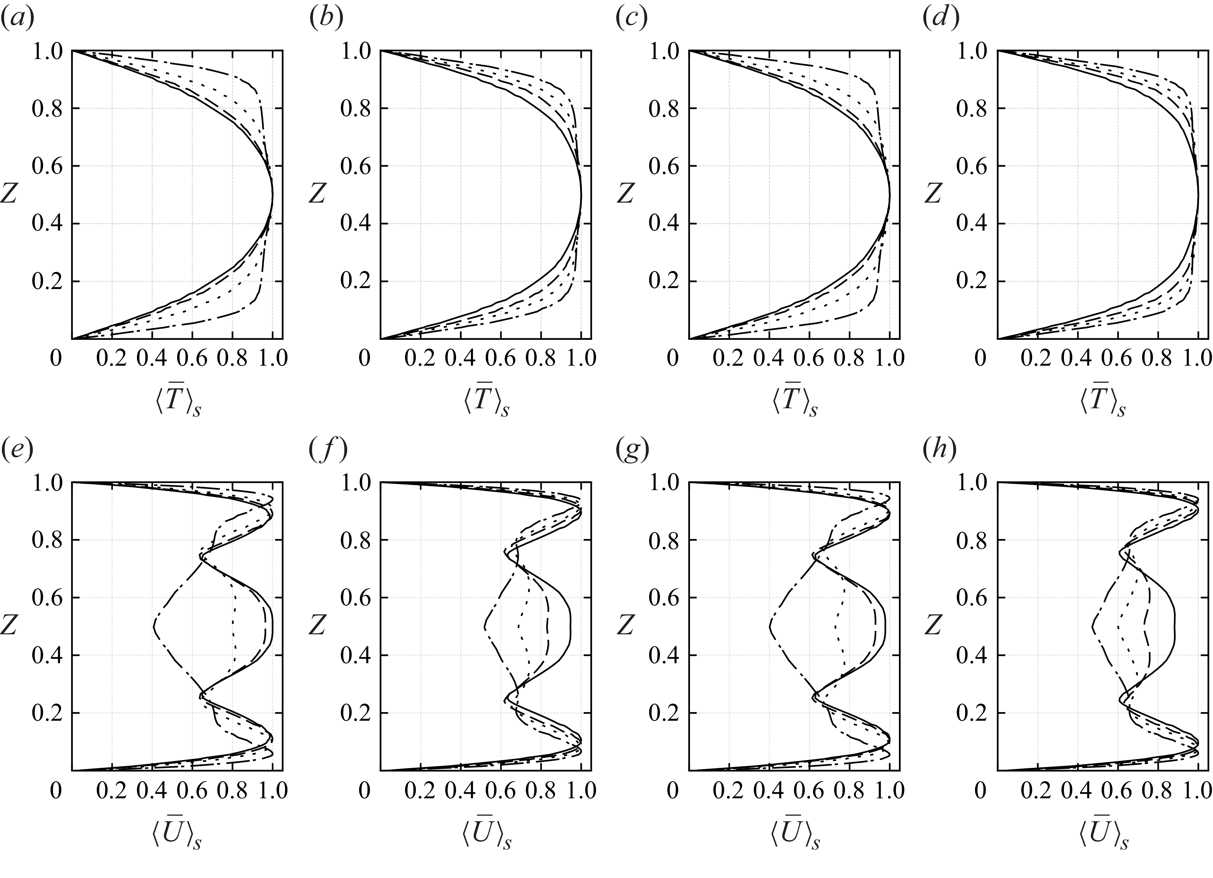
Figure 3. Long description
Eight line graphs show time- and section-averaged temperature and velocity profiles for two fluids, 1-Nonanol and Novec 7200, at different forcing amplitudes. Panel A: Temperature profile for 1-Nonanol at a specific condition. Panel B: Temperature profile for Novec 7200 at a specific condition. Panel C: Temperature profile for 1-Nonanol at another condition. Panel D: Temperature profile for Novec 7200 at another condition. Panel E: Velocity profile for 1-Nonanol at a specific condition. Panel F: Velocity profile for Novec 7200 at a specific condition. Panel G: Velocity profile for 1-Nonanol at another condition. Panel H: Velocity profile for Novec 7200 at another condition. Each panel includes multiple lines representing different forcing amplitudes, with solid, dashed, dotted, and dash-dotted lines indicating varying conditions.
4.3. The BL development and energy dissipation
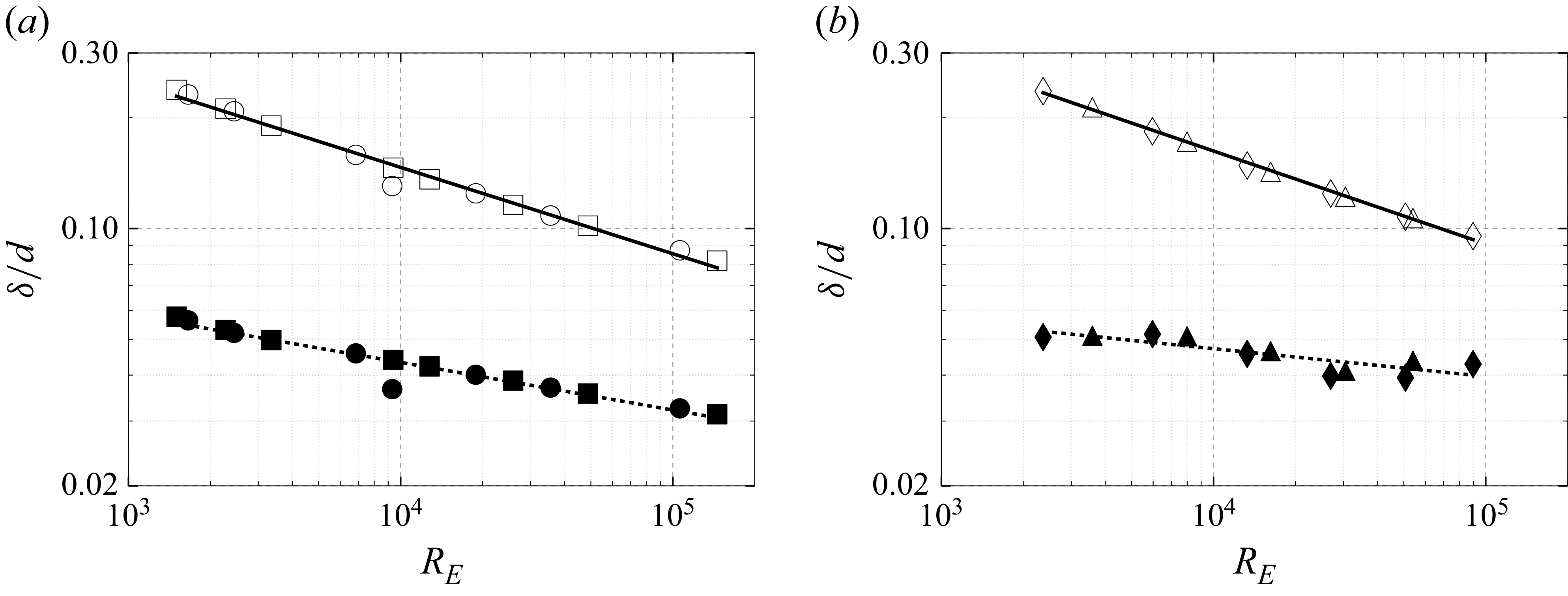
Thermal and kinetic BL thicknesses, normalised by the fluid layer height
 $d$
(
 $\delta _T/d$
and
 $\delta _u/d$
), plotted versus the electric Rayleigh–Roberts number
 $R_E$
. (a) The markers
 $\circ$
and
 $\square$
denote thermal BL thicknesses, and
 $\bullet$
and
 $\blacksquare$
denote kinetic BL thicknesses for 1-Nonanol at 50 Hz and 10 kHz, respectively. (b) The markers
 $\triangle$
and
 $\lozenge$
indicate thermal BL thicknesses, and
 $\blacktriangle$
and
 $\blacklozenge$
indicate kinetic BL thicknesses for Novec 7200 at 50 Hz and 10 kHz, respectively. Power-law fits of
 $\delta _T/d$
(solid lines) and
 $\delta _u/d$
(dashed lines), combining both loss frequencies, are given in (4.3) and (4.4).
The BLs adjacent to the cooled walls play a crucial role in determining the flow and heat transfer dynamics. The thicknesses of the thermal and kinetic BLs are estimated using the slope method, and are denoted by
 $\delta _T$
and
 $\delta _u$
, respectively. The definitions of the thermal and kinetic BL thicknesses are provided in Appendix D. To examine the BL thicknesses within the fluid layer, we use sequential averaging as discussed in § 4.2. The thermal BL thickness
 $\delta _T$
is defined as the intercept of the linear extrapolation of the near-wall temperature gradient with the bulk fluid temperature
 $T_{{bulk}}$
, given by
 \begin{equation} \delta _T = \frac {\delta T}{\left |\partial \langle \overline {T}\rangle _S/\partial z \right |_{wall}}, \end{equation}
where
 $\delta T = \langle \overline {T}\rangle _S(z=0) - T_{{bulk}}$
. The kinetic BL thickness follows an equivalent procedure using the velocity magnitude
 $\langle \overline {U}\rangle _S(z)$
. The kinetic BL thickness is defined as the distance from the wall at which the velocity reaches its maximum value in the bulk flow. The slope method defines
 $\delta _u$
as
 \begin{equation} \delta _u = \frac {\overline {U}_{\textit{max}}}{\left |\partial \langle \overline {U}\rangle _S/\partial z \right |_{wall}}, \end{equation}
where
 $\overline {U}_{\textit{max}}$
is the magnitude of the peak velocity in the bulk of the fluid layer. These definitions provide consistent and reproducible measures of BL thicknesses that relate directly to the local gradients at the boundaries, capturing changes in flow and thermal structure with varying electric forcing. Both of these slope-based definitions are consistent with those employed in Shishkina et al. (Reference Shishkina, Stevens, Grossmann and Lohse2010), where the thermal BL thickness is defined through the inverse wall gradient (slope thickness), and the kinetic BL is defined analogously using the velocity gradient.
Ratio of the thermal to kinetic BL thicknesses,
 $\delta _T/\delta _u$
, versus the electric Rayleigh–Roberts number
 $R_E$
. The markers
 $\circ$
and
 $\square$
represent 1-Nonanol, and
 $\triangle$
and
 $\lozenge$
represent Novec 7200 at 50 Hz and 10 kHz, respectively. Power-law fits of 1-Nonanol (solid line) and Novec 7200 (dashed line) yield
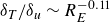 $\delta _T/\delta _u \sim R_E^{-0.11}$
and
 $\delta _T/\delta _u \sim R_E^{{-0.18}}$
, respectively.
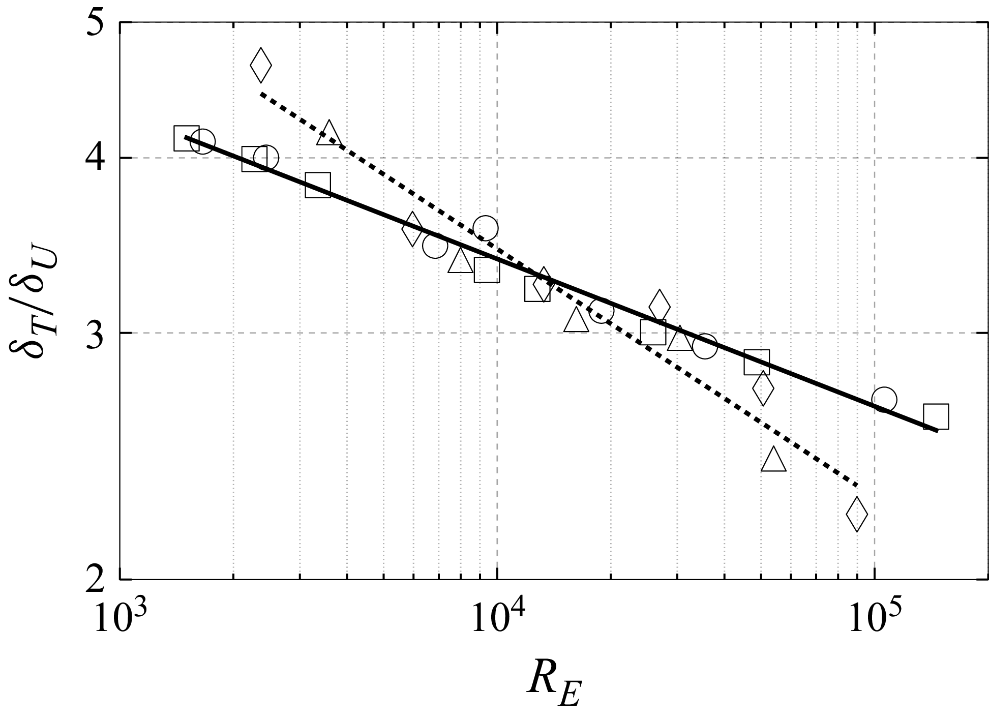
Figure 4 presents the thermal and kinetic BL thicknesses for both working fluids: figure 4(a) for 1-Nonanol, and figure 4(b) for Novec 7200. In both cases, the BL thicknesses decrease with increasing electric Rayleigh–Roberts number, indicating enhanced heat transport. Power-law fits yield the following scaling relations:
 \begin{equation} \delta _T \sim 1.27R_E^{-0.23}, \quad \delta _u \sim 0.143R_E^{-0.13} \quad \text{(1-Nonanol)}, \end{equation}
and
 \begin{equation} \delta _T \sim 1.66 R_E^{-0.25}, \quad \delta _u \sim 0.945 R_E^{-0.08} \quad \text{(Novec 7200)}, \end{equation}
where
 $\delta _T$
decreases more rapidly than
 $\delta _u$
in both fluids. The observed thermal BL scaling follows the same decay as reported by Jawichian et al. (Reference Jawichian, Davoust and Siedel2021), for dielectric fluid under the influence of the DEP force density, with a slight difference in the scaling exponent
 $\pm 0.01$
. To the best of the authors’ knowledge, thermal and kinetic BLs in IH fluids remain unexplored and warrant further investigation.
The observed decay in both power-law slopes (see (4.3) and (4.4)) suggests a possible transition towards the classical BL thicknesses theory of
 $\delta _T\ll \delta _u$
for larger-
 $\textit{Pr}$
fluids. This is also indicated by figure 5, showing the ratio of thermal to kinetic BL thicknesses,
 $\delta _T/\delta _u$
, as a function of the electric Rayleigh–Roberts number
 $R_E$
. The ratio decreases with increasing
 $R_E$
, following power-law scalings
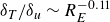 $\delta _T/\delta _u \sim R_E^{-0.11}$
for 1-Nonanol and
 $\delta _T/\delta _u \sim R_E^{-0.18}$
for Novec 7200. Nonetheless, this comes with limitations due to increased electric forcing, discussed in more detail in § 5. To provide an indication of the dimensional values of the BL thickness in a 1-Nonanol fluid layer of height 5 mm at loss frequency 50 Hz and
 $V_E=1900$
(
 $V_0 = 6430$
kV), the thermal and velocity BL thicknesses are given by
 $\delta _T = 7.93 \times 10^{-4}$
and
 $\delta _u = 2.29 \times 10^{-4}$
m, respectively.
The results for the BL indicate that thermal dissipation dominates momentum dissipation within the BL. To elucidate deviations in BL thickness from classical theory, we analyse the time-averaged thermal and kinetic energy dissipation rates, decomposed into bulk and BL contributions. The kinetic energy dissipation is given by
 \begin{equation} \tilde {\varepsilon }_u(\boldsymbol{x},t) = \tilde {\varepsilon }_{u}^{\textit{BL}} + \tilde {\varepsilon }_{u}^{\textit{bulk}} = {\textit{Pr}}^{-1} \langle (\partial _i \overline {u_{\!j}}(\boldsymbol{x} \in \text{BL}))^2 \rangle _V + {\textit{Pr}}^{-1} \langle (\partial _i \overline {u_{\!j}}(\boldsymbol{x} \in \text{bulk}))^2 \rangle _V, \end{equation}
and the thermal energy dissipation reads as
 \begin{equation} \tilde {\varepsilon }_T(\boldsymbol{x},t) = \tilde {\varepsilon }_{T}^{\textit{BL}} + \tilde {\varepsilon }_{T}^{\textit{bulk}} = \langle (\partial _i \overline {T}(\boldsymbol{x} \in \text{BL}))^2 \rangle _V + \langle (\partial _i \overline {T}(\boldsymbol{x} \in \text{bulk}))^2 \rangle _V, \end{equation}
where
 $\boldsymbol{x}$
denotes the spatial position vector, and the conditions
 $\boldsymbol{x} \in \text{BL}$
and
 $\boldsymbol{x} \in \text{bulk}$
indicate that the volume averaging is restricted to the BL and bulk regions, respectively. While the bulk thermal dissipation depends on both thermal diffusion and advection (see (2.14)), Grossmann & Lohse (Reference Grossmann and Lohse2000) showed that in the regime where
 $\delta _T \gt \delta _u$
, it can be approximated analogously to kinetic dissipation. This justifies the decomposition in (4.6).
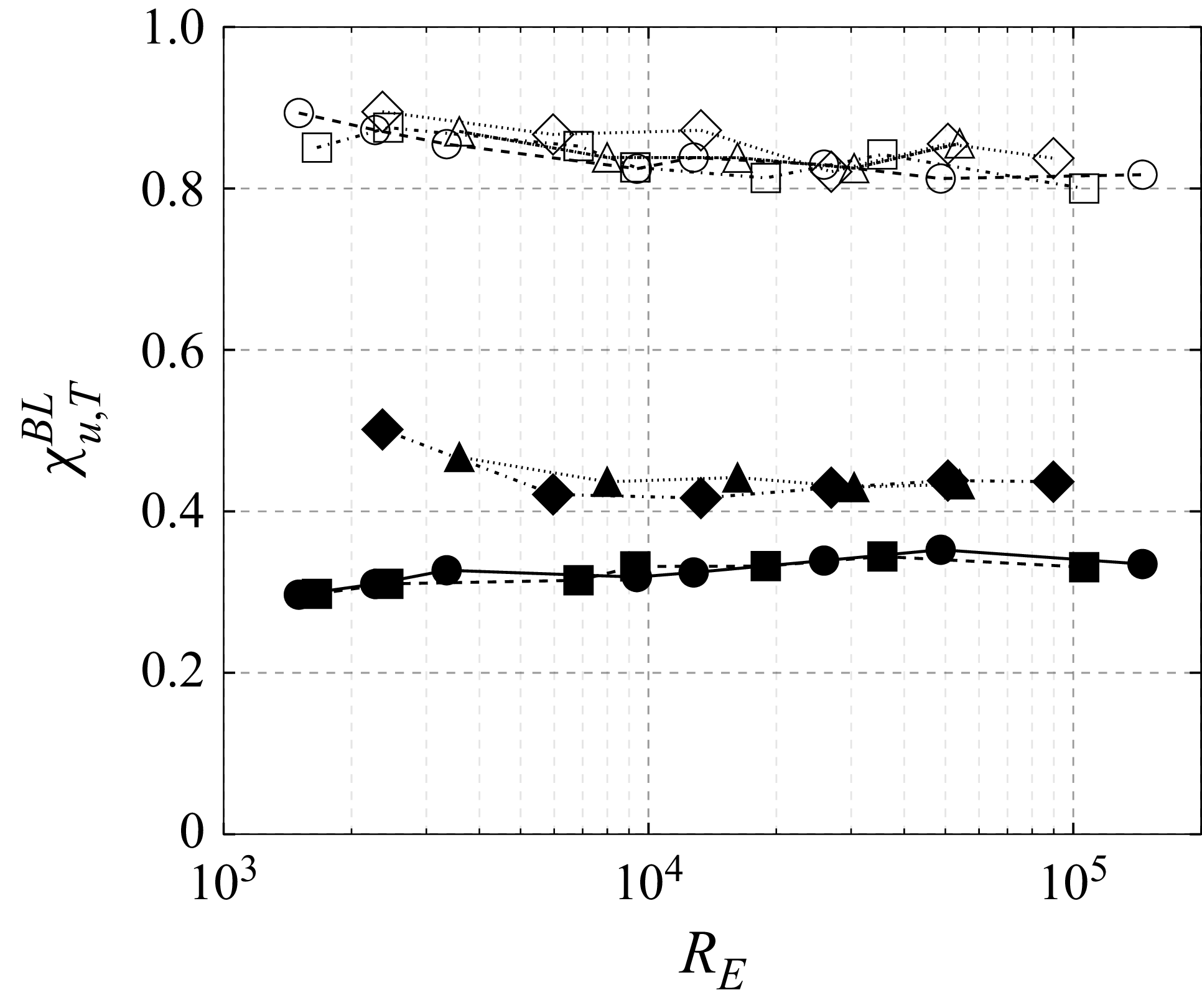
Figure 6 shows the normalised energy dissipation rates in the BL and the bulk regions, defined as
 $\chi _{u}^{\textit{BL}} = \tilde {\varepsilon }_{u}^{\textit{BL}} / \tilde {\varepsilon }_u$
and
 $\chi _{u}^{\textit{bulk}} = \tilde {\varepsilon }_{u}^{\textit{bulk}} / \tilde {\varepsilon }_u$
, respectively. The corresponding ratios for thermal dissipation, denoted with the subscript
 $T$
, are shown analogously. The results confirm that thermal dissipation is predominantly concentrated within the BLs, rather than the bulk, consistent with the evaluated BL thicknesses.
Fraction of energy dissipation rates of the BL fractions of the kinetic energy dissipation rate
 $\chi _{u}^{\textit{BL}} = \tilde {\varepsilon }_{u}^{\textit{BL}} / \tilde {\varepsilon }_{u}$
and thermal dissipation rate
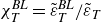 $\chi _{T}^{\textit{BL}} = \tilde {\varepsilon }_{T}^{\textit{BL}} / \tilde {\varepsilon }_{T}$
, plotted as a function of the electric Rayleigh–Roberts number
 $R_E$
. The corresponding dissipation rate fractions for the bulk region can be evaluated, as the sum of
 $\chi _{u}^{\textit{BL}}$
and
 $\chi _{u}^{\textit{bulk}}$
equals unity. The markers for 1-Nonanol at 50 Hz and 10 kHz are
 $\circ$
,
 $\square$
and
 $\bullet$
,
 $\blacksquare$
, while
 $\triangle$
,
 $\lozenge$
and
 $\blacktriangle$
,
 $\blacklozenge$
denote Novec 7200 at 50 Hz and 10 kHz, respectively. The filled markers represent the kinetic dissipation rate, and the empty markers represent the thermal dissipation rate.
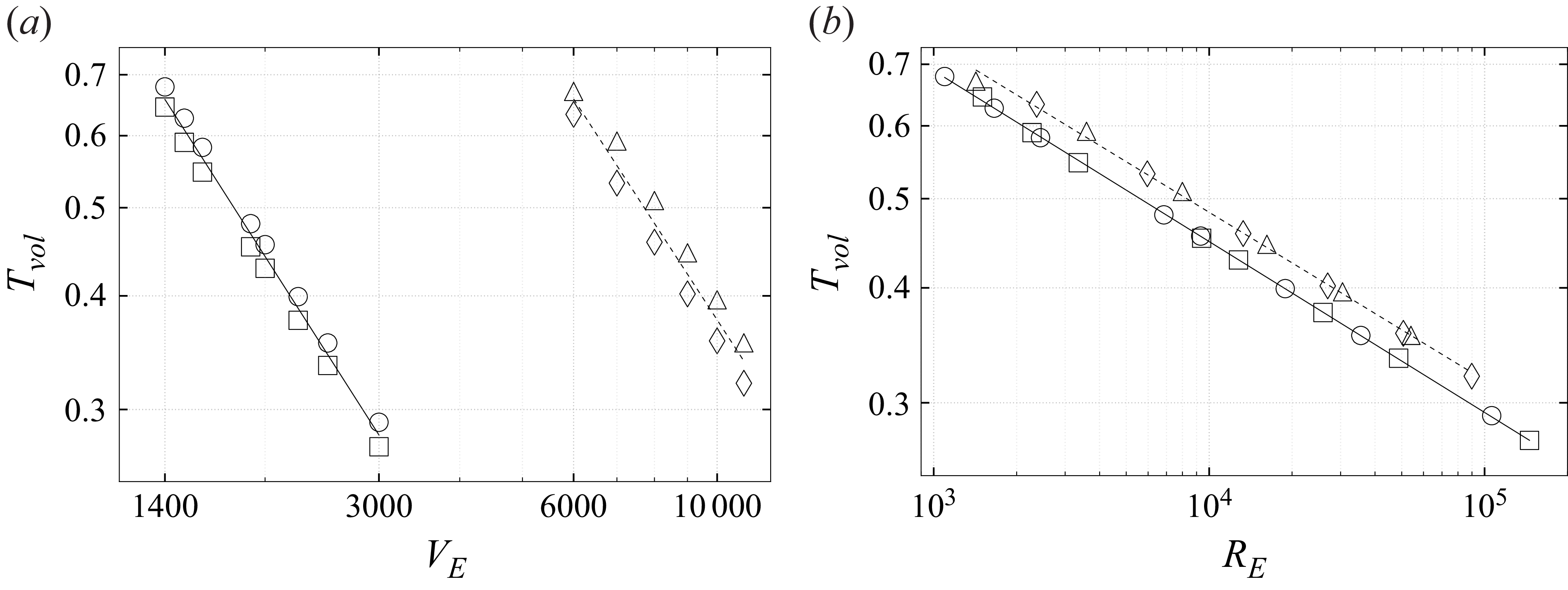
The volume-averaged temperature
 $T_{vol}$
is plotted as a function of (a) the effective voltage
 $V_E$
, and (b) the Rayleigh–Roberts number
 $R_E$
. The markers
 $\circ$
and
 $\square$
represent 1-Nonanol at 50 Hz and 10 kHz, while
 $\triangle$
and
 $\lozenge$
denote Novec 7200 at 50 Hz and 10 kHz, respectively. Power-law fits of
 $T_{vol}$
for 1-Nonanol (solid lines) and for Novec 7200 (dashed lines) are given in (4.7) and (4.8), respectively.
4.4. Convective heat transport and scaling
In the following, we examine the convective heat transport by means of the forcing intensity expressed either by the effective voltage or by the electric Rayleigh–Roberts number. These are given in relation to the volume-averaged temperature, the kinetic energy density and the Nusselt number. The results are compared with established scaling laws in thermal convection, with the main focus on convection in IH fluids.
The volume-averaged temperature
 $T_{vol}$
within the fluid layer is shown in figures 7(a,b) as functions of
 $V_E$
and
 $R_E$
, respectively. For both working fluids,
 $T_{vol}$
decreases with increasing forcing, indicating enhanced advective heat transport in the bulk. Power-law fits yield
 \begin{equation} T_{vol} \sim V_E^{-1.11}, \quad T_{vol} \sim 2.49{R_E}^{-0.19} \quad \text{(1-Nonanol)}, \end{equation}
and
 \begin{equation} T_{vol} \sim V_E^{-1.09}, \quad T_{vol} \sim 2.6 R_E^{-0.18} \quad \text{(Novec 7200)}, \end{equation}
with exponents consistent with those reported by Vilella et al. (Reference Wang, Lohse and Shishkina2018), who found
 $T_{vol} \sim R_E^{-0.192\pm 0.033}$
for
 $R_E \leqslant 5 \times 10^4$
, and
 $T_{vol} \sim R_E^{-0.229\pm 0.003}$
for
 $R_E \geqslant 6.8 \times 10^4$
. Similarly, Wang et al. (Reference Wörner, Schmidt and Grötzbach2021) proposed volume-averaged temperature scaling
 $T_{vol} \sim R_E^{-1/5}$
, consistent with the DNS results of Kazemi et al. (Reference Kazemi, Ostilla-Mónico and Goluskin2022), while a steeper scaling
 $T_{vol} \sim R_E^{-1/4}$
was predicted for larger Prandtl numbers or turbulent regimes. A comparable
 $\sim R_E^{-1/4}$
scaling was also reported by Parmentier & Sotin (Reference Parmentier and Sotin2000) and further discussed by Vilella et al. (Reference Wang, Lohse and Shishkina2018), who suggested that it provides the best fit across their investigated parameter range. The present trends are in line with
 $\sim R_E^{-1/4}$
scaling and with the corresponding scaling observed also for the thermal BLs (see (4.3)–(4.4)).
The kinetic energy density
 $\tilde {E}_K$
is plotted as a function of (a) the effective voltage
 $V_E$
, and (b) the Rayleigh–Roberts number
 $R_E$
. The markers
 $\circ$
and
 $\square$
represent 1-Nonanol at 50 Hz and 10 kHz, while
 $\triangle$
and
 $\lozenge$
denote Novec 7200 at 50 Hz and 10 kHz, respectively. Power-law fits of
 $\tilde {E}_K$
for 1-Nonanol (solid lines) and for Novec 7200 (dashed lines) are given in (4.9) and (4.10), respectively.
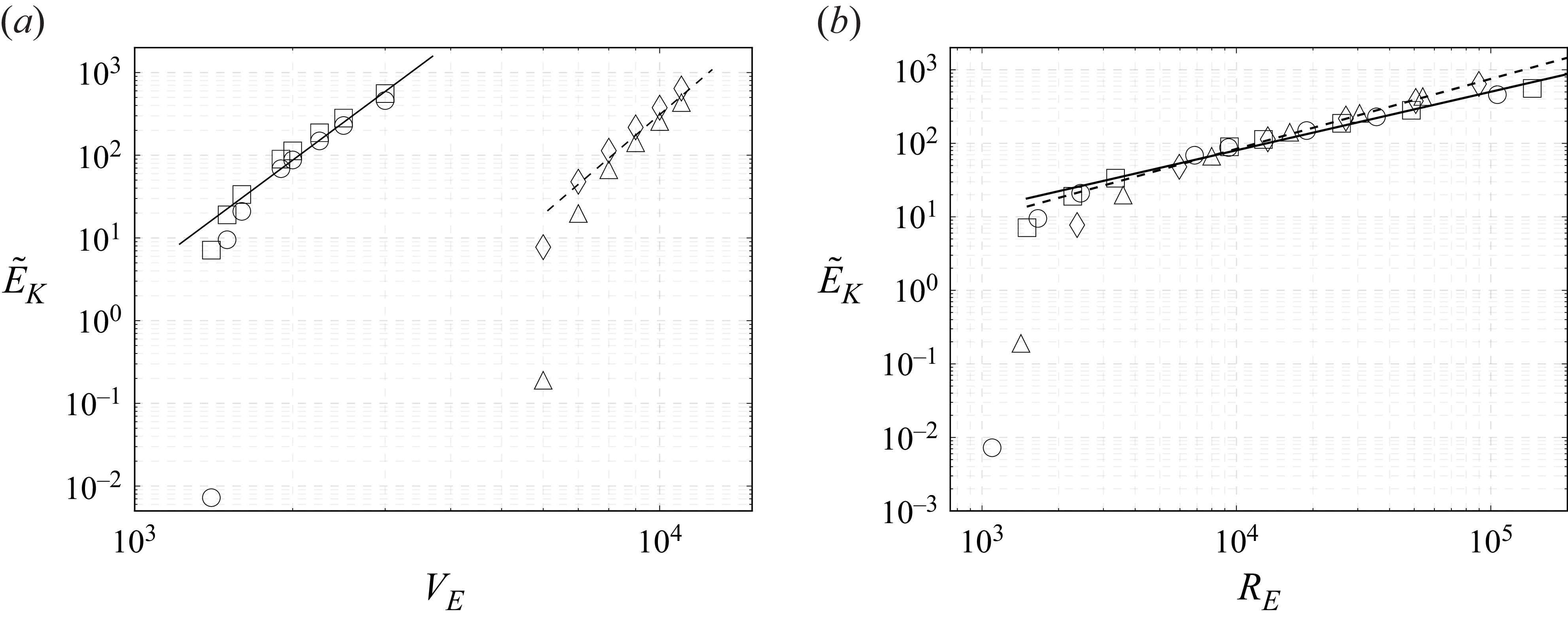
The kinetic energy density
 $\tilde {E}_K$
quantifies the strength of the convective flow and is presented in figures 8(a,b) as functions of
 $V_E$
and
 $R_E$
, respectively. As expected,
 $\tilde {E}_K$
increases with stronger forcing. To relate
 $\tilde {E}_K$
to transport properties, we define the convective Péclet number as
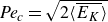 ${\textit{Pe}_c} = \sqrt {2\langle \overline {E_K}\rangle }$
, representing the ratio of advective to thermal transport. The corresponding convective Reynolds number is given by
 ${\textit{Re}_c} = {\textit{Pe}_c} / {Pr}$
, reflecting the balance between advective and viscous effects. Power-law fits yield
 \begin{equation} \tilde {E}_K \sim V_E^{4.71}, \quad \tilde {E}_K \sim R_E^{0.80}, \quad {\textit{Re}_c} \sim R_E^{0.40} \quad \text{(1-Nonanol)}, \end{equation}
and
 \begin{equation} \tilde {E}_K \sim V_E^{5.44}, \quad \tilde {E}_K \sim R_E^{0.95}, \quad {\textit{Re}_c} \sim R_E^{0.475} \quad \text{(Novec 7200)}, \end{equation}
with scaling exponents qualitatively reminiscent of those reported for classical Rayleigh–Bénard convection by Grossmann & Lohse (Reference Grossmann and Lohse2000). However, the present range of
 $R_E$
does not reach the regime in which the Grossmann–Lohse theory is expected to be strictly applicable. Therefore, the comparison should be understood only as a qualitative analogy rather than a direct validation of the predicted Reynolds number scaling exponent of approximately
 $0.5$
for regime
 $I_u$
at moderate Rayleigh numbers and moderate
 $\textit{Pr}$
.
The Nusselt number
 $\textit{Nu}_H$
(see (C1)) characterises the heat transfer intensity and allows correlation with the forcing parameters. In the Kulacki & Goldstein (Reference Kulacki and Goldstein1972) laboratory experiments,
 $\textit{Nu}_H$
was computed separately at the upper and lower boundaries due to asymmetries in heat dissipation. In contrast, under microgravity conditions considered in the present numerical study, no significant difference was observed in
 $\textit{Nu}_H$
between the two boundaries, indicating symmetric thermal behaviour in the absence of Archimedean buoyancy-driven natural convection. Thermal equilibrium is considered established when the relative difference between the heat fluxes at the bounding plates falls below
 $\pm 2\,\%$
. At this point, a time-averaged Nusselt number
 $\textit{Nu}_H^{{av}}$
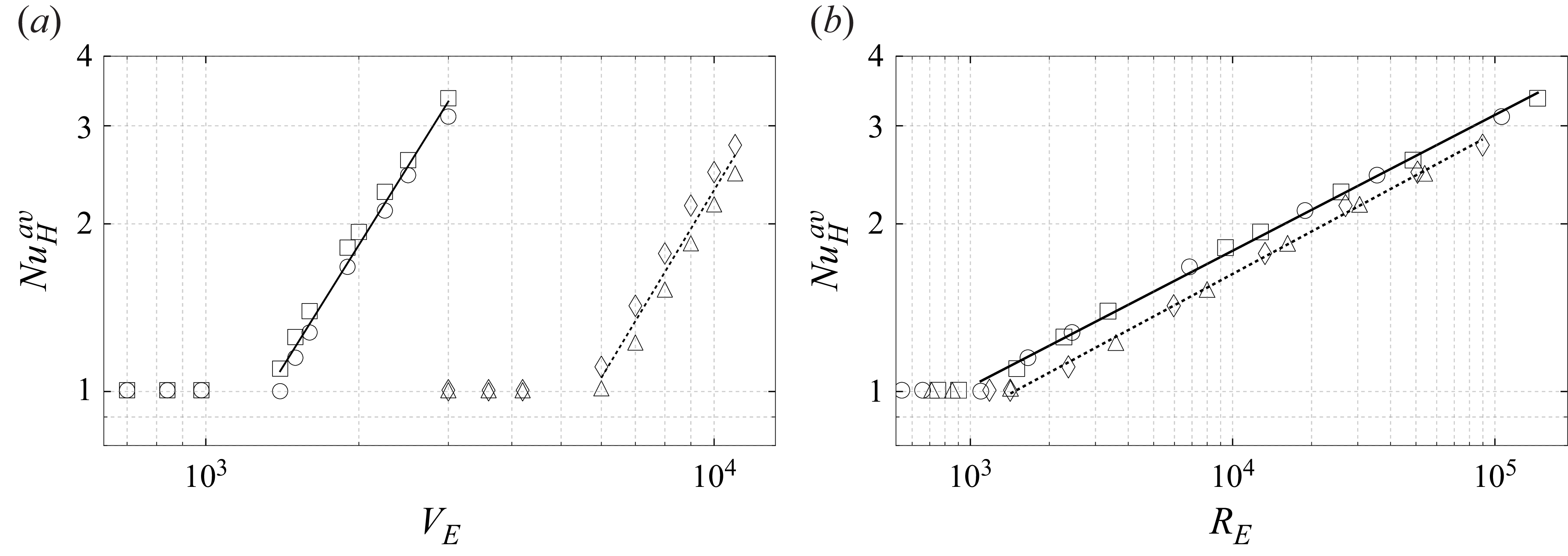
can be evaluated, characterising the mean heat transfer across both boundaries in the IH system. The results for
 $\textit{Nu}_H^{{av}}$
are plotted in figures 9(a,b) as functions of
 $V_E$
and
 $R_E$
, respectively. Power-law fits yield the scalings
 \begin{equation} {\textit{Nu}_H^{{av}} \sim V_E^{1.463 \pm 0.050}, \quad {\textit{Nu}_H^{{av}}} \sim 0.189 R_E^{0.244 \pm 0.004} }\quad \text{(1-Nonanol)}, \end{equation}
and
 \begin{equation} {\textit{Nu}_H^{{av}} \sim V_E^{1.518 \pm 0.105}, \quad {\textit{Nu}_H^{{av}}} \sim 0.158 R_E^{0.253 \pm 0.004}} \quad \text{(Novec 7200)}, \end{equation}
which is consistent with the scaling exponent of
 $R$
ranging from 0.219 to 0.360, reported by Goluskin (Reference Goluskin2016) in their table 3.2.
Figure 9(b) highlights a clear difference in the onset of convection between the two working fluids. This behaviour is consistent with the findings of Yoshikawa et al. (Reference Zaussinger, Haun, Szabo, Travnikov, Al Kawwas and Egbers2020), who showed through a linear stability analysis that variations in the thermoelectric parameter
 $\gamma _e$
shift the critical onset of convection. Our results support this trend, demonstrating that the critical electric Rayleigh–Roberts number
 $ R_E^{crit}$
increases as
 $\gamma _e$
decreases. Since Novec 7200 exhibits a significantly lower
 $\gamma _e$
than 1-Nonanol, convection in Novec 7200 initiates at a higher
 $R_E$
, while 1-Nonanol exhibits an earlier onset.
The average Nusselt number
 $\textit{Nu}_H^{av}$
plotted as a function of (a) the effective voltage
 $V_E$
, and (b) the electric Rayleigh–Roberts number
 $R_E$
. The markers
 $\circ$
and
 $\square$
represent 1-Nonanol at 50 Hz and 10 kHz, while
 $\triangle$
and
 $\lozenge$
denote Novec 7200 at 50 Hz and 10 kHz, respectively. Power-law fits of
 $\textit{Nu}_H^{av}$
for 1-Nonanol (solid lines) and for Novec 7200 (dashed lines) are given in (4.11) and (4.12), respectively.
5. Discussion and limitations
This section compares the present study on internal dielectric heating in fluid layers with previous investigations of IH systems, as well as classical boundary-driven configurations such as Rayleigh–Bénard and TEHD convection.
The present study extends the experimental work of Kulacki & Goldstein (Reference Kulacki and Goldstein1972) and the numerical investigations by Vilella et al. (Reference Wang, Lohse and Shishkina2018) by incorporating internal dielectric heating and thermoelectric coupling, guided by the theoretical framework and linear stability analysis of Yoshikawa et al. (Reference Zaussinger, Haun, Szabo, Travnikov, Al Kawwas and Egbers2020). Comparable scaling laws for IH flows remain limited in the literature. Nevertheless, the observed scaling exponents for thermal BL and
 $T_{vol}$
agree with previous studies (see Kulacki & Goldstein Reference Kulacki and Goldstein1972; Parmentier & Sotin Reference Parmentier and Sotin2000; Moore Reference Moore2008; Vilella et al. Reference Wang, Lohse and Shishkina2018; Wang et al. Reference Wörner, Schmidt and Grötzbach2021; Kazemi et al. Reference Kazemi, Ostilla-Mónico and Goluskin2022).
Notably, we observe
 $\delta _T \gg \delta _u$
for fluids of large Prandtl numbers, where
 $\delta _T \ll \delta _u$
is generally expected in classical boundary-heated systems causing natural convection. However, the explored parameter range, with
 $R_E$
up to
 $10^5$
, remains relatively limited. The notion of a BL implies that its thickness must be much smaller than the characteristic size of the domain. In this regime, the comparatively large thermal diffusivity leads to a thermal BL that is thicker than the velocity BL. This behaviour is consistent e.g. with classical Rayleigh–Bénard convection. The present scaling exponents should therefore be interpreted as indicators of the dominant transport mechanisms over the limited investigated range of
 $R_E$
up to
 $10^5$
rather than as asymptotic laws analogous to larger forcing like Kulacki & Goldstein (Reference Kulacki and Goldstein1972), Vilella et al. (Reference Wang, Lohse and Shishkina2018) or Rayleigh–Bénard convection. Different power laws emerge depending on whether kinetic and thermal dissipation are dominated by the BLs or by the bulk. The corresponding scaling exponents therefore reflect changes in the dominant energy and heat transport balances rather than universal constants. Although the thermal BL thins substantially with increasing forcing, the kinetic BL remains comparatively thick over the accessible parameter range, indicating that the momentum field has not yet reached an asymptotic scaling regime. The observed differences in the exponential decay of the BL ratio indicate a dependence on the Prandtl number, and suggest a transition towards BL thicknesses where
 $\delta _T \ll \delta _u$
, a behaviour characteristic of fluids with higher
 $\textit{Pr}$
and larger
 $R_E$
, but accompanied by constraints discussed in more detail below related to the electric breakdown voltage (see Szabo & Egbers Reference Szabo and Egbers2025). Although the influence of the forcing parameter
 $\gamma _e$
is not addressed here for larger values, its potential impact warrants further investigation.
To study BL thicknesses for larger values in
 $R_E$
for the expected intercept of power laws as discussed above may not be feasible, as it is in contrast to the dielectric breakdown voltage. For typical commercially available dielectric fluids, electric Rayleigh numbers for boundary-heated fluid layers range from
 $10^4$
to
 $10^5$
and are currently achievable in laboratory environments (see Barry et al. Reference Barry, Kang, Yoshikawa and Mutabazi2023; Kang et al. Reference Kang, Mutabazi and Yoshikawa2024; Szabo & Egbers Reference Szabo and Egbers2025). The dielectric breakdown voltage of these fluids depends on their polarity and insulating behaviour. Polar fluids, such as hydrofluoroethers (e.g. Novec 7200), exhibit slightly lower breakdown voltages approximately
 $23.8$
kV mm−1. Although these fluids are still effective insulators, their inherent polarity contributes to a modest decrease in dielectric strength. Strongly polar fluids, such as 1-Nonanol (an alcohol-based liquid), demonstrate even lower breakdown thresholds, approximately
 $20.7$
kV mm−1, due to their increased conductivity and interaction with electric fields. A range of factors can affect the breakdown performance of dielectric fluids, including the presence of moisture, contaminants, electrode configuration and experimental set-up. Overall, non-polar fluids are typically favoured for high-voltage uses due to their superior insulation properties. To enhance the electric Rayleigh–Roberts number, various frequency ranges of the applied alternating electric voltage can be examined in order to identify the maximum loss factor, thereby extending the feasible range of the forcing parameter.
The convective Reynolds number scales as
 $\textit{Re}_c\sim R_E^{0.400-0.475}$
, which is qualitatively similar to the
 $\textit{Re}_c\sim Ra^{0.5}$
dependence predicted by the Grossmann & Lohse (Reference Grossmann and Lohse2000) theory for Rayleigh–Bénard convection, although the accessible forcing range remains well below the asymptotic regime where that theory is expected to apply. This similarity suggests that the increase in kinetic energy is primarily associated with the strengthening of the large-scale circulation for relative small
 $R_E$
rather than with a transition to turbulence.
The thermal BL scaling, the reduction of the volume-averaged temperature, the increase in the convective Reynolds number and the increase in the Nusselt number are mutually consistent. As
 $R_E$
increases, stronger convective motion enhances advective transport within the bulk, reducing
 $T_{vol}$
while simultaneously thinning the thermal BL. Since the conductive resistance of the BL decreases with decreasing
 $\delta _T$
, the resulting increase in heat transfer naturally produces the observed
 $\textit{Nu}_H^{av}$
scaling. In particular, the resulting scaling exponent aligns remarkably well with previous laboratory studies of IH fluids conducted under gravity conditions, and is comparable in magnitude to the classical Rayleigh–Bénard scaling exponent
 $0.25$
(see Kulacki & Goldstein Reference Kulacki and Goldstein1972; Grossmann & Lohse Reference Grossmann and Lohse2000).
However, no significant variation in the scaling exponents is observed with respect to
 $\textit{Pr}$
in the range of explored parameters. This suggests that within the investigated parameter range, the DEP force density primarily governs the large-scale circulation, while molecular diffusivities mainly influence the prefactors rather than the scaling exponents. Whether this behaviour persists at larger
 $R_E$
or reflects the limited range of accessible forcing remains an open question.
One has to note that for boundary-heated fluid layers, Jawichian et al. (Reference Jawichian, Davoust and Siedel2021) observed no significant dependence of
 $\textit{Pr}$
on
 $\textit{Nu}_B$
at large electric Rayleigh numbers denoted in their study by variable
 $L$
. This finding contrasts with classical natural convection, where
 $\textit{Nu}_B$
typically scales with both
 $Ra$
and
 $\textit{Pr}$
. For example, Tritton (Reference Trowbridge, Melosh, Steckloff and Freed1977) provides
 ${\textit{Nu}_B} = f({Ra, Pr})$
, while Grossmann & Lohse (Reference Grossmann and Lohse2000) reported a scaling
 ${\textit{Nu}_B} \sim {Ra}^{1/4}\, {\textit{Pr}}^{-1/12}$
for
 ${Pr} \gtrsim 1$
. This raises questions about the governing diffusion mechanisms in TEHD convection, both in the bulk and within the BLs. However, previous studies have reported a dependence on
 $\textit{Pr}$
away from the onset of TEHD convection. The classical numerical study of the onset of TEHD convection by Yoshikawa et al. (Reference Yoshikawa, Kang, Mutabazi, Zaussinger, Haun and Egbers2013b
) (see their figure 7) also indicated a
 $\textit{Pr}$
dependence at larger electric Rayleigh numbers, but the trend is not clearly given. Szabo & Egbers (Reference Szabo and Egbers2025) have shown a
 $\textit{Pr}$
dependence using an electrode configuration similar to that reported in Jawichian et al. (Reference Jawichian, Davoust and Siedel2020); a similar observation was made by Travnikov et al. (Reference Travnikov, Crumeyrolle and Mutabazi2015) in cylindrical annuli. In the latter, the influence of
 $\textit{Pr}$
on
 $\textit{Nu}_B$
varied in addition with the radius ratio
 $\eta$
, with more pronounced effects at smaller
 $\eta$
, particularly closer to the onset of convection. Notably, all studies incorporate thermoelectric feedback via the parameter
 $\gamma _e$
in the electrostatic Gauss equation, which is known to influence the onset and heat transfer in TEHD convection demonstrated in planar layers (see Yoshikawa et al. Reference Yoshikawa, Kang, Mutabazi, Zaussinger, Haun and Egbers2013b
), cylindrical geometries (see Travnikov et al. Reference Travnikov, Crumeyrolle and Mutabazi2015, Reference Travnikov, Crumeyrolle and Mutabazi2016) and dielectrically heated fluids (see Yoshikawa et al. Reference Zaussinger, Haun, Szabo, Travnikov, Al Kawwas and Egbers2020).
6. Conclusion
The behaviour of two distinct Prandtl number fluids subjected to dielectric heating in a confined fluid layer, cooled from opposite bounding plates, was explored through 3-D numerical simulations under microgravity conditions. The resulting convective structures were categorised based on their temporal and topological behaviour into four groups as the electric Rayleigh–Roberts number increased: stable hexagonal patterns, mixed hexagonal-square structures, dominant rectangular patterns and time-dependent convection. The spatial distribution of temperature and velocity, averaged over cross-sections, displayed the structural differences between the groups.
Scaling laws were formulated for key dimensionless quantities, including volume-averaged temperature and kinetic energy density, the convective Reynolds number and the Nusselt number, correlating with simulation results across a two-orders-of-magnitude range in the electric Rayleigh–Roberts number. The variation in the onset of convection was associated with the thermoelectric parameter, showing a shift in the critical threshold. Our findings confirm this trend, that the critical electric Rayleigh–Roberts number increases as the thermoelectric parameter decreases.
Acknowledgements
The authors want to thank A. Meyer, O. Crumeyrolle, I. Mutabazi and U. Harlander for fruitful discussions about convection in dielectric heated fluid layers, and V. Motuz and M. Hamede, who are pursuing the experimental realisation of the present study.
Funding
This work was supported by four research projects. The projects ‘AtmoFlow’ (grant nos 50WP2209, 50WM1841, 50WM2141 and 50WM2441), ‘TEKUS’ and its successor ‘DEPIC’ (grant nos 50WP1644, 50WM1944 and 50WM2244) and ‘AID2’ (grant no. 50WM2354) were funded by the German Federal Ministry for Economic Affairs and Climate Action (BMWK) through the German Aerospace Centre (DLR). The authors further acknowledge support from the German Federal Ministry of Education and Research, and the German federal states as part of the National High-Performance Computing (NHR) joint funding programme under grant no. bbi00021 (http://www.nhr-verein.de/en/our-partners).
Declaration of interests
The authors report no conflict of interest.
Author contributions
P.S.B.S.: conceptualisation, methodology, validation, formal analysis, investigation, resources, data creation, writing original and final draft, review and editing, visualisation, project administration, funding acquisition. K.N.: methodology, conceptualisation, investigation, numerical simulations, formal analysis, data creation, visualisation, validation, review and editing, preparation of draft. Y.A.M.: numerical simulations, data creation, preparation of draft. M.S.: preparation of draft. C.E.: project administration, funding acquisition. F.Z.: review and editing, visualisation. All authors have read and agreed to the published version of the paper.
Appendix A. Fluid properties
The physical properties of the two working fluids used in this study, Novec 7200 and 1-Nonanol, are summarised in table 2. These include the thermophysical and dielectric properties evaluated at the reference temperature
 $T_0$
, listed along with the characteristic time scales and the resulting Prandtl numbers.
Appendix B. Numerical implementation and discretisation
The simulations are performed using a finite-volume technique within OpenFOAM v2012, employing a custom-modified buoyantPimpleFoam solver (Gaillard et al. Reference Gaillard, Szabo and Egbers2024, Reference Gaillard, Szabo, Travnikov and Egbers2025). The numerical procedure consists of two stages. In the first stage, the energy equation (2.14) and Gauss’s law (2.15) are solved to obtain the initial electrostatic and thermal fields. The resulting electric field gradient is subsequently used to initialise the fully coupled, transient computation of the velocity, pressure, temperature and electric potential fields.
Spatial discretisation follows established second-order-accurate schemes. Divergence terms are approximated using the Gauss linear scheme, while Laplacian terms are treated with the Gauss linear corrected formulation to ensure accuracy on non-orthogonal meshes. Surface-normal gradients are evaluated using the corrected option within snGradSchemes, reducing numerical diffusion. Field interpolation is performed using the linear scheme, and gradients are computed via the leastSquares method for robustness on irregular meshes. Temporal integration is carried out using a second-order Crank–Nicolson scheme with blending factor 0.9, providing a balance between stability and temporal accuracy in transient simulations.
The pressure equation is solved using the geometric–algebraic multi-grid (GAMG) solver. The momentum and energy equations are handled using the preconditioned bi-conjugate gradient stabilised (PBiCGStab) solver with a diagonal incomplete LU (DILU) preconditioner, which is well suited for non-symmetric systems. The electric potential equation is solved separately using GAMG with diagonal incomplete Cholesky (DIC) smoothing and forward DIC (FDIC) preconditioning.
The coupling between pressure and velocity is achieved via the pressure-implicit with splitting of operators (PIMPLE) algorithm. The electric field and corresponding DEP force density are updated at each outer PIMPLE iteration. Multiple non-orthogonal correction steps and residual controls are employed to ensure numerical stability and convergence. All simulations are parallelised using OpenMPI, as implemented natively in OpenFOAM.
Appendix C. Benchmark validation and mesh-independence study
Prior to the present investigation, the numerical solver was validated for natural convection and TEHD convection in a series of benchmark studies (Gaillard et al. Reference Gaillard, Szabo and Egbers2024, Reference Gaillard, Szabo, Travnikov and Egbers2025), demonstrating deviations of less than 1 % when compared with pseudo-spectral and finite-element solutions.
To further validate the numerical approach for a non-isothermal fluid layer, we perform additional benchmark simulations using the configuration of Barry et al. (Reference Barry, Kang, Yoshikawa and Mutabazi2023). The boundary conditions follow equations (3a)–(3d) and (7a)–(7b) of that study. We consider a commercial silicone oil with Prandtl number
 $\textit{Pr}=65$
and electric permittivity
 $\gamma _e = 0.03$
. The heat transfer is quantified by the Nusselt number
 \begin{equation} \textit{Nu}_B = \frac {\dot {q}_{t}}{\dot {q}_{c}}, \end{equation}
where
 $\dot {q}_{t}$
denotes the total heat flux, and
 $\dot {q}_{c}$
denotes the conductive heat flux across the differentially heated, adiabatic boundaries. For the benchmark case discussed in § 3.4,
 $\dot {q}_{c}$
is given analytically by
 $\dot {q}_{c} = k \Delta T / d$
, while
 $\dot {q}_{t}$
is obtained numerically. In boundary-heated fluid layers,
 $\textit{Nu}_B = 1$
corresponds to purely conductive transport, whereas
 $\textit{Nu}_B \gt 1$
indicates convective enhancement. Figure 10(a) shows
 $\textit{Nu}_B$
for equilibrated flow states as a function of the electric Rayleigh number
 \begin{equation} L = \frac {\alpha\, \Delta T\, g_e d^3}{\nu \kappa }, \end{equation}
where
 $g_e$
is the electric gravity evaluated at the reference position defined in equation (4) of Barry et al. (Reference Barry, Kang, Yoshikawa and Mutabazi2023). The results exhibit excellent agreement with the reference data over the entire parameter range, with deviations remaining below
 $1\,\%$
even at the highest Rayleigh numbers.
(a) The Nusselt number
 $\textit{Nu}_B$
for equilibrated flow states as a function of the boundary heated electric Rayleigh number
 $L$
at
 $\textit{Pr} = 65$
and
 $\gamma _e = 0.03$
. This is shown for comparison with figure 5 in Barry et al. (Reference Barry, Kang, Yoshikawa and Mutabazi2023) (
 $\blacksquare$
denote simulation data; black line for Barry et al. (Reference Barry, Kang, Yoshikawa and Mutabazi2023), where the definition of
 $L$
is found). (b) Mesh independence study: kinetic energy density
 $\tilde {E}_{K}$
(
 $\blacksquare$
) and volume-averaged temperature
 $T_{vol}$
(
 $\square$
), plotted as functions of the total number of cells at
 $R_E = 7 \times 10^6$
.

The computational domain shown in figure 1 is discretised using OpenFOAM’s built-in blockMesh generator. Uniform cell spacing is employed in the bounding plate direction, while boundary-layer refinement in the wall-normal direction is achieved using a simple grading scheme with refinement ratio 0.1. This ensures adequate resolution of near-wall gradients while maintaining computational efficiency.
Mesh-convergence is achieved for meshes with at least xCells = 200, yCells = 200 and zCells = 40, corresponding to approximately
 $3.2\times 10^{4}$
cells for the 2-D geometry, and
 $1.6\times 10^{6}$
cells for the 3-D geometry. Mesh-independence tests indicate deviations of less than 2 % in key global quantities, such as the kinetic and thermal energy densities, as illustrated in figure 10(b).
Appendix D. The BL thickness
The thermal and kinetic BL thicknesses are denoted by
 $\delta _T$
and
 $\delta _u$
, and calculated using a linear approximation by using the slope method introduced by Shishkina et al. (Reference Shishkina, Stevens, Grossmann and Lohse2010). Before calculating the BL thickness, the 3-D fields are first temporal averaged and then spatial averaged via sections first in the
 $y{-}z$
plane and then in the
 $x{-}z$
plane, denoted by
 $\langle {\cdot }\rangle _S$
to evaluate the wall near fields. For the thermal BL thickness, a first-order Taylor expansion gives
 \begin{equation} \langle \overline {T}\rangle _S(z) \approx \langle \overline {T}\rangle _S(z=0) + \left . \frac {\partial \langle \overline {T}\rangle _S}{\partial z} \right |_{wall}, \end{equation}
and at
 $z=\delta _t$
,
 $\langle \overline {T}\rangle _S(z)$
becomes
 \begin{equation} \overline {T}_{\textit{bulk}} \approx \langle \overline {T}\rangle _S(z=0) + \left . \frac {\partial \langle \overline {T}\rangle _S}{\partial z} \right |_{wall} \delta _t. \end{equation}
By rearranging, we obtain
 \begin{equation} \delta _T = \frac {\overline {T}_{\textit{bulk}}-\langle \overline {T}\rangle _S(z=0)}{\left |\partial \overline {T}/\partial z \right |_{wall}} \quad \Rightarrow \quad \delta_T =\frac {\delta T}{\left |\partial \overline {T}/\partial z \right |_{wall}}, \end{equation}
which is the thermal BL thicknesses. Similarly, the kinetic BL thickness is where the flow reaches the maximum of the velocity magnitude,
 $\overline {U}_{max}$
:
 \begin{equation} \langle \overline {U}\rangle _S(z) \approx \langle \overline {U}\rangle _S(z=0) + \left . \frac {\partial \langle \overline {U}\rangle _S}{\partial z} \right |_{wall} z. \end{equation}
For the no-slip boundary condition
 $\overline {U}(z=[0,1]) = 0$
,
 \begin{equation} \langle \overline {U}\rangle _S(z) \approx \left . \frac {\partial \langle \overline {U}\rangle _S}{\partial z} \right |_{wall} z, \end{equation}
and we obtain
 \begin{equation} \overline {U}_{\textit{max}} \approx \left . \frac {\partial \langle \overline {U}\rangle _S}{\partial z} \right |_{wall} \delta _u \quad \Rightarrow \quad \delta _u = \frac {\overline {U}_{\textit{max}}}{ \left |\partial \langle \overline {U}\rangle _S/\partial z \right |_{wall}}, \end{equation}
which is the thicknesses of the kinetic BL. Both of these slope-based definitions are consistent with those employed in Shishkina et al. (Reference Shishkina, Stevens, Grossmann and Lohse2010), where the thermal BL thickness is defined via the inverse wall gradient (slope thickness), and the kinetic BL thickness is defined analogously using the velocity gradient.
Schematics of the slope-fitting procedure for determining the (a) thermal and (b) kinetic BL thicknesses. The time- and section-averaged profiles are shown by solid lines, the linear fits by dashed lines, the BL thicknesses by dotted lines, and the bulk profiles by dash-dotted lines, according to Shishkina et al. (Reference Shishkina, Stevens, Grossmann and Lohse2010).


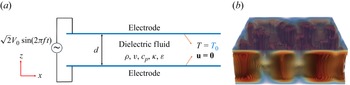
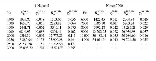
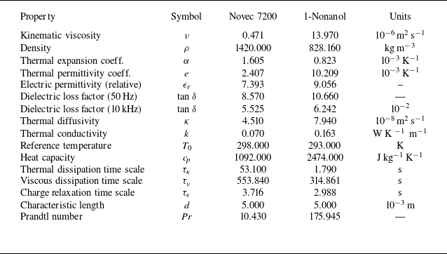
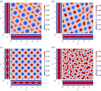
 T
 x
 y
 z
 VE=1500
 RE=1657
 VE=1600
 RE=2441
 VE=1900
 RE=6846
 VE=3000
 RE=106096
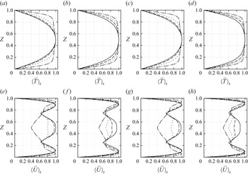
 ⟨T¯⟩S(z)
 ⟨U¯⟩S(z)
 50Hz
 50Hz
 10kHz
 10kHz
 VE=1500
 7000
 VE=1600
 8000
 VE=1900
 9000
 VE=3000
 11000
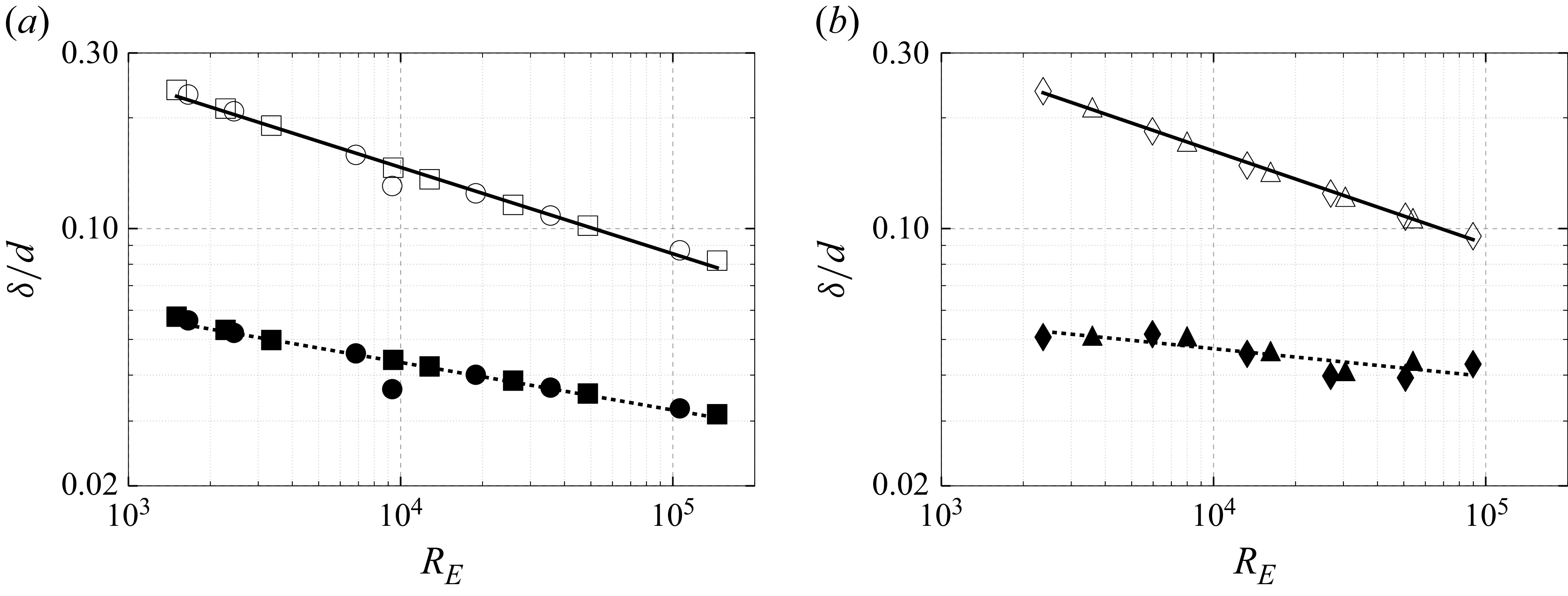
 d
 δT/d
 δu/d
 RE
 ∘
 ◻
 ∙
 ◼
 △
 ◊
 ▴
 ⧫
 δT/d
 δu/d
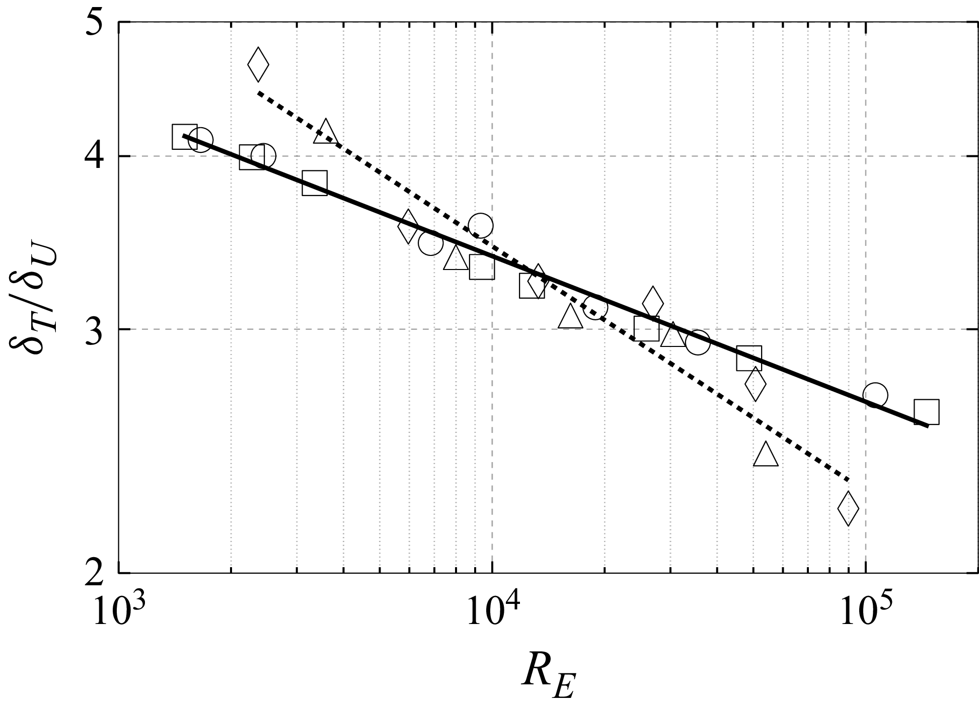
 δT/δu
 RE
 ∘
 ◻
 △
 ◊
 δT/δu∼RE−0.11
 δT/δu∼RE−0.18
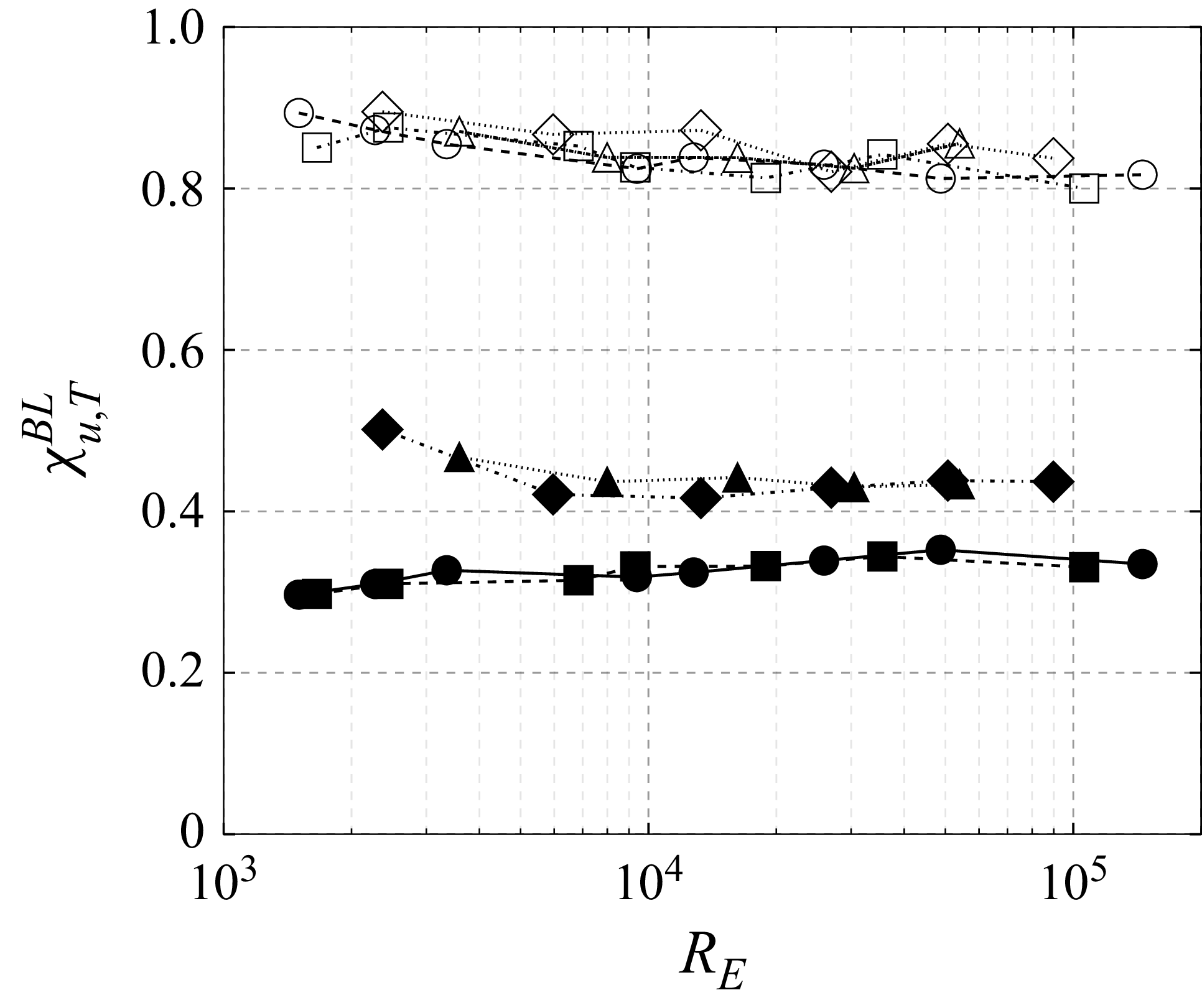
 χuBL=ε~uBL/ε~u
 χTBL=ε~TBL/ε~T
 RE
 χuBL
 χubulk
 ∘
 ◻
 ∙
 ◼
 △
 ◊
 ▴
 ⧫
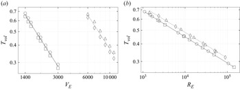
 Tvol
 VE
 RE
 ∘
 ◻
 △
 ◊
 Tvol
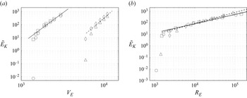
 E~K
 VE
 RE
 ∘
 ◻
 △
 ◊
 E~K
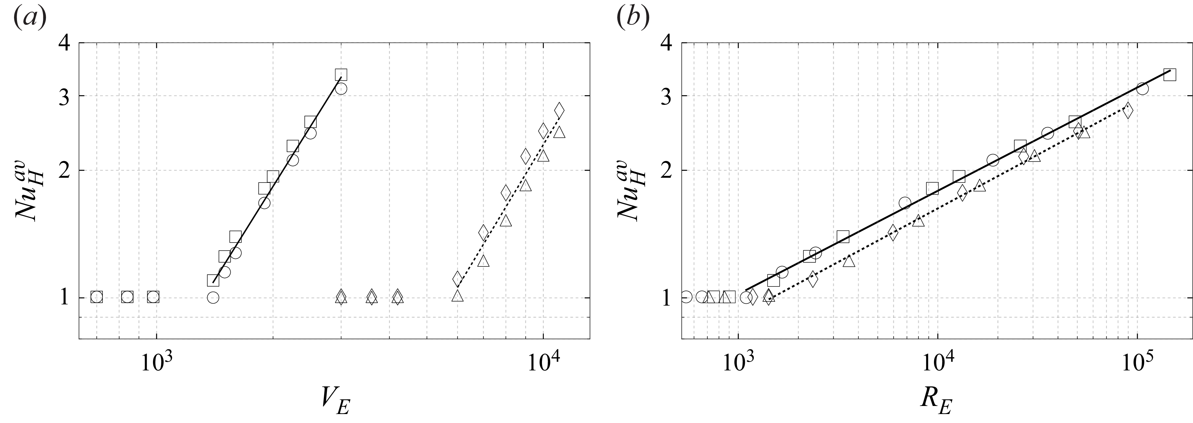
 NuHav
 VE
 RE
 ∘
 ◻
 △
 ◊
 NuHav
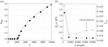
 NuB
 L
 Pr=65
 γe=0.03
 ◼
 L
 E~K
 ◼
 Tvol
 ◻
 RE=7×10⁶
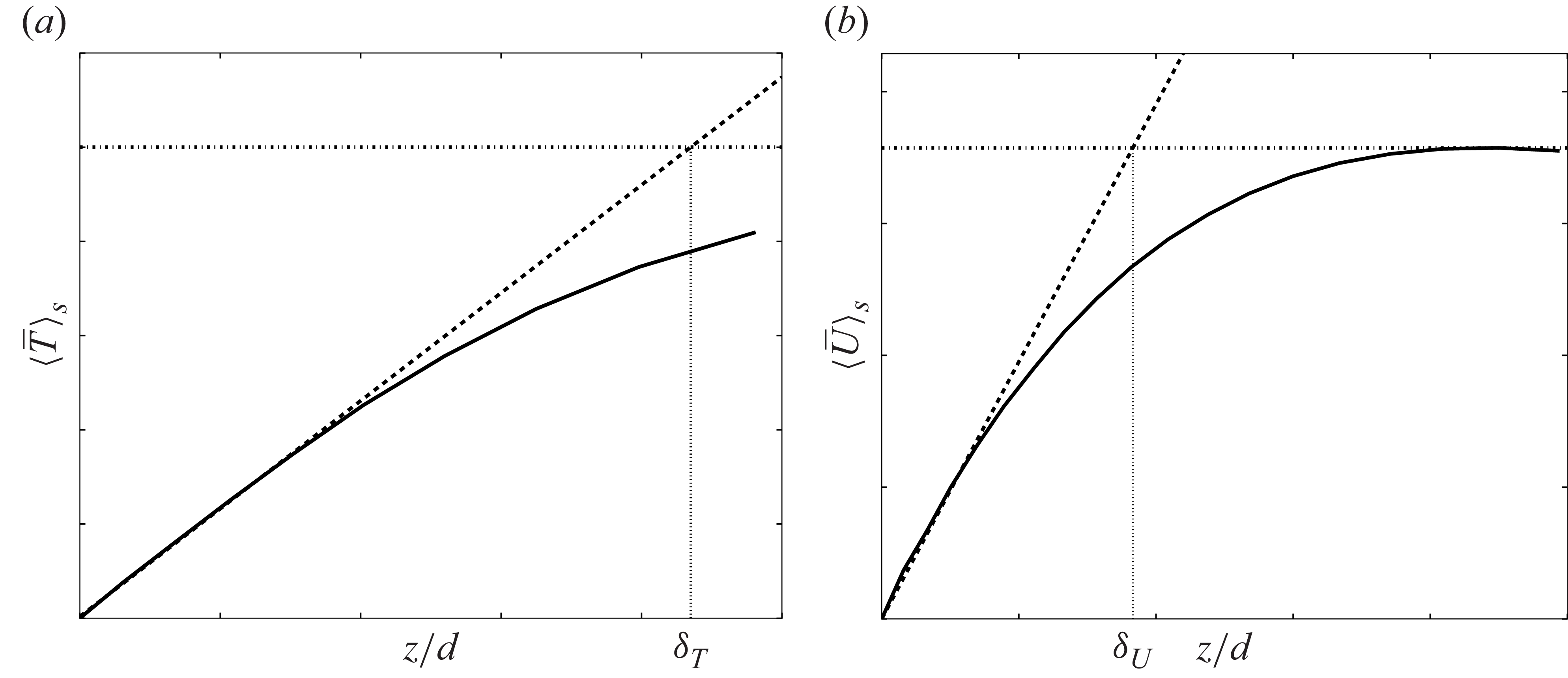

 Open access

