





1. Introduction
The world is experiencing multiple simultaneous shifts in the planetary environmental system, the global human energy infrastructure, the international security system, the global economic system, and the information system, which could give rise to a profound polycrisis (Lawrence et al., Reference Lawrence, Homer-dixon, Janzwood, Rockstöm, Renn and Donges2024). In this context, the need to address intertwined economic, social, and environmental problems has given rise to the notion of just sustainability transitions, understood as processes of transformative change aimed at enabling present and future human and non-human living beings to survive and flourish (Avelino et al., Reference Avelino, Wijsman, Van Steenbergen, Jhagroe, Wittmayer, Akerboom, Bogner, Jansen, Frantzeskaki and Kalfagianni2024).
Already in 1992 the Union of Concerned Scientists issued a ‘warning to humanity’, which was reiterated in 2017 and signed by 13,524 researchers across the world (Ripple et al., Reference Ripple, Wolf, Newsome, Galetti, Alamgir, Crist, Mahmoud and Laurance2017). Further warnings concerning the ‘climate emergency’ (Cavicchioli et al., Reference Cavicchioli, Ripple, Timmis, Azam, Bakken, Baylis, Behrenfeld, Boetius, Boyd, Classen, Crowther, Danovaro, Foreman, Huisman, Hutchins, Jansson, Karl, Koskella, Mark Welch and Webster2019; Ripple et al., Reference Ripple, Wolf, Gregg, Levin, Rockström, Newsome, Betts, Huq, Law, Kemp, Kalmus and Lenton2022, Reference Ripple, Wolf, Gregg, Rockström, Newsome, Law, Marques, Lenton, Xu, Huq, Simons and King2023, Reference Ripple, Wolf, Gregg, Rockström, Mann, Oreskes, Lenton, Rahmstorf, Newsome, Xu, Svenning, Pereira, Law and Crowther2024), the threats to mountain ecosystems (Schmeller et al., Reference Schmeller, Urbach, Bates, Catalan, Cogălniceanu, Fisher, Friesen, Füreder, Gaube, Haver, Jacobsen, Le Roux, Lin, Loyau, Machate, Mayer, Palomo, Plutzar, Sentenac and Ripple2022) and insects (Harvey et al., Reference Harvey, Tougeron, Gols, Heinen, Abarca, Abram, Basset, Berg, Boggs, Brodeur, Cardoso, de Boer, De Snoo, Deacon, Dell, Desneux, Dillon, Duffy, Dyer and Chown2023), the bidirectional impacts between climate change and microorganisms (Cavicchioli et al., Reference Cavicchioli, Ripple, Timmis, Azam, Bakken, Baylis, Behrenfeld, Boetius, Boyd, Classen, Crowther, Danovaro, Foreman, Huisman, Hutchins, Jansson, Karl, Koskella, Mark Welch and Webster2019), the threats to ecosystems posed by invasive alien species (Pyšek et al., Reference Pyšek, Hulme, Simberloff, Bacher, Blackburn, Carlton, Dawson, Essl, Foxcroft, Genovesi, Jeschke, Kühn, Liebhold, Mandrak, Meyerson, Pauchard, Pergl, Roy, Seebens and Richardson2020), and on affluence as a barrier to sustainability (Wiedmann et al., Reference Wiedmann, Lenzen, Keyßer and Steinberger2020) have emphasized the urgency of a just transition.
Thus, time emerges as a key variable in the quest for sustainability. With every year of delayed climate action, the emission pathways consistent with international climate goals become steeper or depend more on large-scale negative emissions to achieve ‘net zero’ (cf. IPCC, 2018). The existence of nonlinear dynamics and different critical thresholds suggests that if the transition occurs too slow or too late, anthropogenic pressure on the Earth system could result in irreversible changes with long-term negative impacts on human development (Lenton et al., Reference Lenton, Rockström, Gaffney, Rahmstorf, Richardson, Steffen and Schellnhuber2019). Therefore, transition scenarios in the literature are generally modeled as early transitions, with decisive changes occurring decades before, rather than after, 2050 (e.g. IEA, 2022; IPCC, 2018).
However, despite the proliferation of multilateral environmental agreements (Mitchell et al., Reference Mitchell, Andonova, Axelrod, Balsiger, Bernauer, Green, Hollway, Kim and Morin2020) and numerous transition efforts at the local level (Ehnert et al., Reference Ehnert, Egermann and Betsch2022; Frantzeskaki et al., Reference Frantzeskaki, Dumitru, Anguelovski, Avelino, Bach, Best, Binder, Barnes, Carrus, Egermann, Haxeltine, Moore, Mira, Loorbach, Uzzell, Omann, Olsson, Silvestri, Stedman and Rauschmayer2016), a global societal transition has yet to materialize. Instead, greenhouse gas emissions are at an all-time high (Ripple et al., Reference Ripple, Wolf, Gregg, Rockström, Mann, Oreskes, Lenton, Rahmstorf, Newsome, Xu, Svenning, Pereira, Law and Crowther2024) and significant transgressions for six out of nine planetary boundaries have pushed the Earth system far beyond the ‘safe operating zone’ known to be conducive to human welfare and societal development (Richardson et al., Reference Richardson, Steffen, Lucht, Bendtsen, Cornell, Donges, Drüke, Fetzer, Bala, von Bloh, Feulner, Fiedler, Gerten, Gleeson, Hofmann, Huiskamp, Kummu, Mohan, Nogués-bravo and Rockström2023).
Because economic production remains tightly linked to material flows, preventing high rates of absolute decoupling (Haberl et al., Reference Haberl, Wiedenhofer, Virág, Kalt, Plank, Brockway, Fishman, Hausknost, Krausmann, Leon-gruchalski, Mayer, Pichler, Schaffartzik, Sousa, Streeck and Creutzig2020; Martinico-Perez et al., Reference Martinico-Perez, Schandl, Fishman and Tanikawa2018; Streeck et al., Reference Streeck, Wiedenhofer, Krausmann and Haberl2020; Vogel & Hickel, Reference Vogel and Hickel2023), the past decade has seen a surge in theoretical and modeling work exploring new economic development paradigms centered on the universal satisfaction of basic human needs within planetary boundaries (Brand-Correa & Steinberger, Reference Brand-Correa and Steinberger2017; Dixson-Declève et al., Reference Dixson-Declève, Gaffney, Ghosh, Randers, Rockström and Stoknes2022; Fanning & Raworth, Reference Fanning and Raworth2025; Hickel, Reference Hickel2019; Kallis et al., Reference Kallis, Hickel, O'Neill, Jackson, Victor, Raworth, Schor, Steinberger and Ürge-Vorsatz2025; Millward-Hopkins et al., Reference Millward-Hopkins, Steinberger, Rao and Oswald2020; Stoknes et al., Reference Stoknes, Collste, Cornell, Callegari, Spittler, Gaffney and Randers2025). These approaches imply strong intra- and international convergence processes of per capita consumption to relatively low levels, and a fundamental reorientation of economic processes and policies away from the ‘growth paradigm’ (Schmelzer, Reference Schmelzer2017).
Although such alternative proposals are gaining traction both in academia and policy-making (Engler et al., Reference Engler, Kretschmer, Rathgens, Ament, Huth and von Wehrden2024; Kallis et al., Reference Kallis, Mastini and Zografos2024), an ambitious and coherent implementation implies deep structural changes on the global level, including a new Earth governance structure that enforces resource extraction caps, accompanied by capital redistribution and other social policies, and in the absence of a series of positive ‘black swans’ or social tipping points, it seems improbable that such a new world order will emerge within the next two decades (cf. Biermann et al., Reference Biermann, Abbott, Andresen, Bäckstrand, Bernstein, Betsill, Bulkeley, Cashore, Clapp, Folke, Gupta, Gupta, Haas, Jordan, Kanie, Kluvánková-oravská, Lebel, Liverman, Meadowcroft and Zondervan2012; Fitzpatrick et al., Reference Fitzpatrick, Parrique and Cosme2022; Lauer & Llases, Reference Lauer and Llases2025a). At the same time, the increase in climate-change-induced disasters and catastrophes under certain conditions might open up new windows of opportunity for societal change (Brundiers & Eakin, Reference Brundiers and Eakin2018; Matsuura, Reference Matsuura2022; Rizzo et al., Reference Rizzo, Cappellano, Pierantoni and Sargolini2022), which, in the best case, could result in a global transition, albeit with a delay of various decades compared to timely transitions occurring under ideal conditions.
Therefore, in this paper we aim to explore how the timing of a global sustainability transition influences socioeconomic and environmental outcomes. While the cost of delayed climate action has already been examined in various scenario exercises (e.g. Aryanpur et al., Reference Aryanpur, Balyk, Glynn, Gaur, McGuire and Daly2024; Schaeffer et al., Reference Schaeffer, Gohar, Kriegler, Lowe, Riahi and Van Vuuren2015; Winning et al., Reference Winning, Price, Ekins, Pye, Glynn, Watson and McGlade2019), little is known about delayed ‘radical’ sustainability pathways characterized by a degrowing global economy and large-scale redistribution measures. Consequently, we are particularly interested in the following research questions:
1. How might socioeconomic, demographic, and environmental developments differ under an early global just sustainability transition compared to a delayed transition?
2. Which trade-offs might appear in an early versus a late transition?
3. To what extent does the timing of the transition influence the long-term stability and resilience of the emerging socioeconomic system?
To examine these questions, we conduct a quantitative modeling study grounded in two previously developed qualitative scenarios, which we parameterize and simulate using a newly developed Integrated Assessment Model (IAM). We present and discuss the main scenario results and conclude by outlining potential avenues for future research.
2. Methods
2.1. Scenario and model selection
We select two previously developed qualitative storylines (Lauer et al., Reference Lauer, de Castro and Carpintero2025; Lauer & Llases, Reference Lauer and Llases2025a) called Fast Sustainability Transition 5: sufficiency economies (FST5) and Business as usual – Global Emergency Governance (BAU-GEG) that serve as examples for an ‘early’ and a ‘late’ societal transition.
In FST5, a black swan in the form of a successful global movement triggers various social tipping points that result in the establishment of a Planetary Confederation in 2032. Legitimated by a global consensus for egalitarian wealth and resource distribution, as well as ecological technology development, the Planetary Confederation implements ambitious social, economic, demographic, environmental, and technological policies which fundamentally change the world system during the 21st century.
In BAU-GEG, the world follows its historical development pathway characterized by weak environmental and social policies. However, as environmental conditions deteriorate and economic crises increase, legitimation for the world economic system and the institutions that support it dwindles. Under the pressure of an organized global worker movement, a world emergency regime is installed that pushes stringent environmental, social, and demographic policies, focusing on minimizing resource use and pollution, disaster management, and the fulfillment of human needs.
Three main reasons motivated our choice of scenarios.
First, both are of global scale and provide relatively detailed information on social, (geo)political, economic, and environmental variables and their interlinkages. One scenario represents an ‘ideal’, intentional, swift, and early transition while the other illustrates a delayed transition that only occurs as biophysical limits to growth emerge, political tensions increase, and social forces have built up enough pressure to impose radical changes at the global level. Their similarity in scale and variables, combined with the difference in the timing of the transition, renders them particularly suitable for a comparative scenario analysis.
Second, they feature nonlinear changes in key variables that are assumed to be influenced by strong social, ecological, environmental, and demographic policies. Therefore, the transition in the selected scenarios is not limited to the technological realm. Notably, both can be classified as ‘post-growth’ scenarios as they foresee a reduction in the consumption level of richer classes, a more equitable access to resources and economic goods, and a change in production patterns to reduce human impacts on Earth systems (Edwards et al., Reference Edwards, Brockway, Bickerstaff and Nijsse2025; Van Eynde et al., Reference Van Eynde, Dillman, Vogel and O'Neill2025). Hence, they are built on the basic premise that ultimately neither continued environmental degradation nor environmental restoration are compatible with permanently increasing consumption levels. Last, both scenarios are linked to a relatively extensive scenario translation protocol, which facilitates the quantification process and renders the parametrization of the scenarios more transparent.
For the scenario quantification, we use the system-dynamics-based simulation model MORDRED (Model Of Resource Distribution and Resilient Economic Development). MORDRED was built following various calls in the literature for more heterogeneous and diverse futures that break with the ‘continuity bias’ and integrate systemic shocks as well as alternative economic paradigms and systems (Hickel et al., Reference Hickel, Brockway, Kallis, Keyßer, Lenzen, Slameršak, Steinberger and Ürge-Vorsatz2021; Lauer et al., Reference Lauer, de Castro and Carpintero2024; Raskin & Swart, Reference Raskin and Swart2020; Rothman et al., Reference Rothman, Raskin, Kok, Robinson, Jäger, Hughes and Sutton2023). The model has been developed within the tradition of macroeconomic and climate change modeling through IAMs (Fernández-Villaverde et al., Reference Fernández-Villaverde, Gillingham and Scheidegger2025) and of ecological macroeconomic modeling (Hardt & O'Neill, Reference Hardt and O'Neill2017). Specifically, it combines monetary input–output modeling with system dynamics and thus shares structural similarities with other models belonging to this modeling family (Briens, Reference Briens2015; Cordier et al., Reference Cordier, Uehara, Weih and Hamaide2017; Nieto et al., Reference Nieto, Carpintero, Lobejón and Miguel2020). Within the IAM tradition, similar, albeit technically more complex, models include MEDEAS (Capellán-Pérez et al., Reference Capellán-Pérez, de Blas, Nieto, de Castro, Miguel, Carpintero, Mediavilla, Lobejón, Ferreras-alonso, Rodrigo, Frechoso and Álvarez-Antelo2020) and WILIAM (Lifi et al., Reference Lifi, de Blas, Capellan-perez, Mediavilla, Miguel, Parrado-hernado, Llases, Álvarez-Antelo, Calleja, Wergles, Ferreras, Ramos, Arto, Calheiros, Capela Lourenco, Morlin, D'alessandro, van Allen, Eggler and Oakes2023; Mediavilla et al., Reference Mediavilla, Lifi, Ferreras-Alonso, Miguel and De Blas2025). Although MORDRED has a lower level of representation of technological systems, it features a high level of disaggregation in the socioeconomic and demographic realms, which sets it apart from most existing IAMs.
MORDRED differs from IAMs developed outside of system dynamics through its high number of endogenously evolving, interlinked variables and its attention to different economic input factors that might limit economic growth. MORDRED’s key strengths include its modular structure, the option to activate different feedback mechanisms, as well as the user-friendly programming software (Vensim), which allows the model to be tailored to different scenarios by adapting the simulation time and adding necessary new variables. Another important characteristic of the model is its level of abstraction that renders the representation of different economic systems feasible. This makes it possible to create scenarios involving a change in the economic system. Collectively, MORDRED’s structural characteristics facilitate the simulation of nonlinear futures with strong deviations from historical trends and render the model suitable for the quantification of the selected transition scenarios.
MORDRED consists of several interlinked modules, the principal ones being the demographic, economic, labor, land, energy, and climate modules. The demographic module calculates changes in the world population, which consists of 20 age cohorts and 3 world regions: the ‘center’, covering all high-income countries, the ‘semiperiphery’, which includes all upper-middle-income countries, and the ‘periphery’, containing the lower-middle- and low-income countries. Changes in the demographic module influence the labor module by changing the labor supply, which consists of the segment of the world population aged 15–64, as well as the economy module via changes in the final demand for different products. At the same time, changes occurring in the economic module, such as changes in production and consumption per capita, impact age-specific mortality and fertility rates in the demographic module. The economic, labor, land, and energy modules are linked via sectoral labor, land, and energy intensities. As human labor, different land types (forest, land for renewable energy generation, land for food cultivation, land classified as ‘other land’ by FAO) and different energy types (fossil fuels, bioenergy, fossil-based-, and non-fossil-based electricity) are necessary input factors into the economic process, they can act as limiting factors to growth if the required inputs to meet global demand for economic goods exceed the available stock of input factors. Last, the economic module influences the climate module via different greenhouse gas emissions, primarily caused by the combustion of fossil fuels, while changes in the climate module impact the economic module through climate damages that increase nonlinearly with global average temperatures.
The economic module is based on an input–output framework (Miller & Blair, Reference Miller and Blair2009). Thus, it differentiates between different final demand components (private consumption, public consumption, and gross fixed capital formation) and sectoral demands for intermediate goods that are disaggregated into 25 sectors. Given that one of the core concerns behind the development of MORDRED was to explore inequality in consumption and living standards, the model disaggregates private (household) consumption within the global economy into nine classes: The richest 20%, poorest 30%, and the remaining middle class of the center (R20C, P30C, and M50C), the richest 20%, poorest 30%, and the remaining 50% of the semiperiphery (R20S, P30S, and M50S), as well as the richest 20%, poorest 30%, and the remaining middle class of the periphery (R20P, P30P, and M50P).
In order to conduct the simulations, we created two new model versions, MORDRED 1.1.5 and 1.1.6, which differ slightly from the original 1.0 version. The two model versions allow us to differentiate between technological, economic, demographic, and social developments before and after the transition starts. Additionally, we partly endogenized changes in the intensity of land used to grow food, land used economically for forestry, and land classified as ‘other land’ by the FAO in both model versions. Finally, we added an endogenous component to the evolution of sectoral labor intensities in the model version used to simulate the BAU-GEG scenario. The default simulation time in the model covers the period 2019–2100, which we adopt, since we consider the period long enough to show the most significant changes caused by transition policies as well as differences between an early and a late transition. A detailed description of MORDRED 1.0 and its data sources, as well as the 25 economic sectors integrated in the model, is given in Lauer and Llases (Reference Lauer and Llases2025b). Additionally, the Supplementary Material (SM) relates the model structure to the literature, points out benefits and limitations of the chosen modeling approaches, and presents the main causal loop diagrams for the most important modules. Equally, the SM contains a comprehensive table listing all exogenous parameters, their numeric values, and a short justification for each value.
2.2. Scenario parametrization
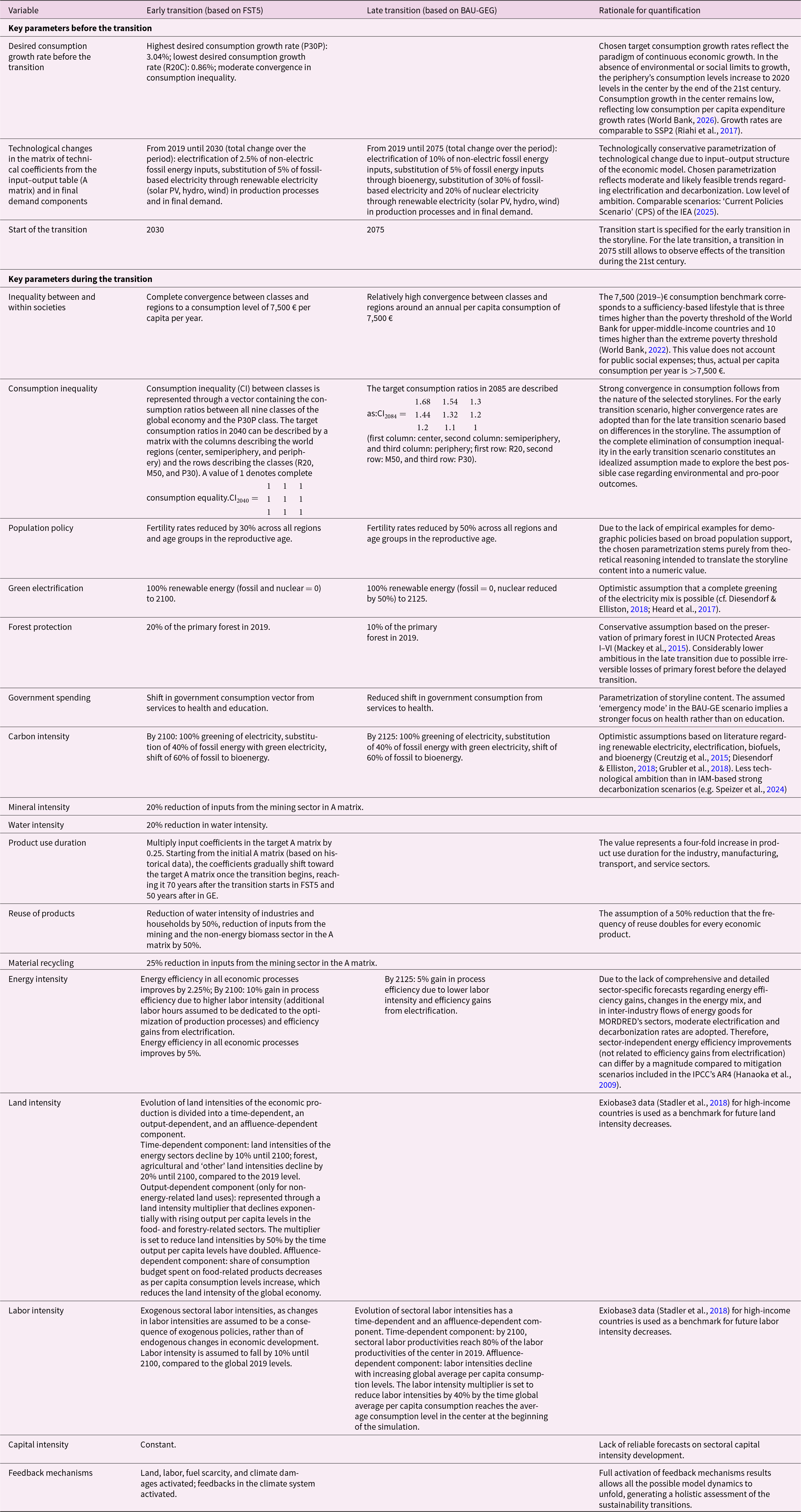
By comparing the scenario storylines and the scenario parametrization protocols provided for FST5 and BAU-GEG with the capacity of MORDRED to represent the envisioned changes (cf. SM Section 2), we developed a list of variables that are at the same time represented by the model and relevant for both scenario storylines. Subsequently, the selected variables were parametrized considering the information provided in the translation protocols (Table 1). To increase the comparability between the scenarios and highlight differences caused by the timing of the transition, we selected rather similar technological and socioeconomic parameter values. Notable differences include a higher birth reduction policy and a lower primary forest protection policy in BAU-GEG, compared to FST5. Also, while social redistribution policies occur within 10 years after the beginning of the transition in both scenarios, technological changes such as changes in the energy mix take 70 years in the FST5 scenarios and only 50 years in the BAU-GEG, reflecting higher urgency.
Parametrization of the two selected qualitative scenarios

Table 1 Long description
Scenario parameters compare an early versus late sustainability transition across consumption growth, technology change, inequality, population policy, energy mix, resource intensities, and model boundary conditions. Before transition, the early case assumes higher desired consumption growth in the global periphery and low growth in the center, while the late case follows a business-as-usual style pathway. Technology shifts are modest in both, but the early case concentrates changes between 2019 and 2030, whereas the late case spreads larger electrification and renewable substitution out to 2075. Transition timing differs sharply: 2030 for early versus 2075 for late. During transition, both aim for strong convergence toward about 7,500 euros per person per year, but the early case assumes complete elimination of consumption inequality, while the late case retains noticeable gaps between regions and income groups. Population policy is stronger in the late case, with a larger fertility reduction than in the early case. Electricity becomes fully renewable by 2100 in the early case, while the late case reaches full renewables later and keeps some nuclear for longer; forest protection is also weaker in the late case. Several circular-economy and intensity measures are specified mainly for the early case, and some late-case entries are not provided, so comparisons are incomplete for minerals, water, and recycling. Rationale notes that many choices are intentionally conservative or optimistic to translate qualitative storylines into feasible numeric assumptions.
The start of the transition was set to 2030 for FST5, following the information in the scenario storyline. Conversely, as no specific timeframe is given for the BAU-GEG scenario, we chose 2075 as the starting point, which on the one hand constitutes a significant delay relative to the ‘early’ transition, but on the other hand still allows us to explore possible changes caused by the ‘late’ transition during the last 25 years of the simulation period.
3. Results
To compare the two scenarios, we organize the simulation results into three categories: (i) socioeconomic and demographic variables, (ii) biophysical variables, and (iii) system-level indicators from which we can draw hypotheses regarding the stability of the world system toward the end of the simulation and beyond the simulation period. To describe the scenarios, we will use ‘FST5/early-transition scenario’ and ‘BAU-GEG/late-transition scenario’ interchangeably.
3.1. Socioeconomic performance
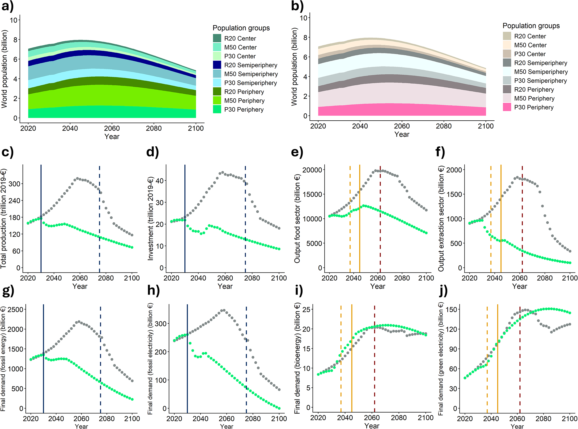
The evolution of socioeconomic variables is comparable in both scenarios until the moment when transition policies are implemented in the early-transition scenario (Figure 1). In FST5, a population policy that reduces birth rates across all world regions and age groups in the reproductive age (15–44), combined with rising per capita consumption levels of the poorer social classes, results in a world population peak in 2033 and a steady decline afterward to 4.86 billion in 2100. Conversely, in the BAU-GEG scenario, world population starts to level off in the 2060s and declines significantly during the late transition period between 2075 and 2100 due to the strong population policy, resulting in a population of 6.63 billion in 2100. Overall, significant changes in population size across the center, semiperiphery, and periphery occur during both scenarios (Figure 1a and b). While the population trend is negative in both scenarios in the center, with an early transition accelerating the decline, in the semiperiphery and periphery the early transition leads to an earlier peak in population, which, in the case of the middle class of the periphery, is about half a billion lower than in the late-transition scenario. Already in 2019, the center is by far the smallest world region, and the difference grows over time in both scenarios. For example, in the late-transition scenario, at the start of the simulation, the size of the wealthiest 20% of the semiperiphery is still slightly smaller than half of the center's population (559 million compared to 620 million people). However, by the end of the simulation, the smallest class in the semiperiphery exceeds the biggest class in the center by almost 100 million people (410 vs. 318 million). Similarly, while the middle class of the periphery in the early-transition scenarios approaches the initial size at the end of the simulation, the size of the semiperiphery’s middle class is reduced by 50% compared to 2019. Both the general decrease in world population and the relative increase in the size of classes with lower consumption levels drive reductions in total final demand, causing a slowdown of environmental degradation. As output and investment ultimately depend on final consumption demands, the evolution of the variables in Figure 1c–f can be better understood in the context of demographic changes. Both total production and investment drop strongly during the global redistribution phase between 2030 and 2040 in the early-transition scenario as global consumption demands are reorganized. Once the target consumption rate is reached across all social classes, total output and investment decline steadily until the end of the population, driven by the decline in world population. Importantly, the output of the food sector increases during the transition period and only reaches its peak in 2049 (Figure 1e). This is explained by the fact that the poorest classes spend a larger share of their consumption budget on food. Only as consumption levels continue to increase does this share start to shrink, eventually causing production in this sector to peak. Conversely, output in the mining and non-fossil extraction sector decreases faster than in other sectors due to the assumed technological changes that reduce the dependency of the economy on the extractive sector (Figure 1f).
Evolution of the main demographic and macroeconomic indicators for the early (green) and late (grey) transition scenario. (a) World population in the early transition; (b) world population in the late transition; (c) world output; (d) gross fixed capital formation; (e) output of the food sector; (f) output of the non-fossil fuel extraction sector; (g) final demand for non-electric fossil energy; (h) final demand for fossil-based electricity; (i) final demand for biomass-based non-electric energy; and (j) final demand for renewable-based electricity. Solid vertical lines refer to the early-transition scenario, whereas dashed vertical lines refer to the late-transition scenario. Blue lines mark the start of the transition, orange lines indicate when the 2°C threshold is crossed, and the red line indicates when the 3°C threshold is crossed (only occurs in the late transition scenario).

Figure 1 Long description
Multiple line graphs labeled a) to j), each representing different indicators over time from 2020 to 2100. Graph a) shows world population in billions for the early transition scenario, with population groups such as R20 Center, M50 Center, and P30 Center for the center region, and equivalent R20/M50/P30 groups for the semiperiphery and periphery. The x-axis is the year and the y-axis is population in billions. Graph b) displays the same for the late transition scenario. Graph c) illustrates world output in million 2019-euros, with the x-axis as the year and the y-axis as total production in million 2019-euros. Graph d) shows gross fixed capital formation in billion 2019-euros, with the x-axis as the year and the y-axis as investment in billion 2019-euros. Graph e) represents output of the food sector in billion 2019-euros, with the x-axis as the year and the y-axis as output in billion 2019-euros. Graph f) shows output of the non-fossil fuel extraction sector in billion 2019-euros, with the x-axis as the year and the y-axis as output in billion 2019-euros. Graph g) depicts final demand for non-electric fossil energy in billion 2019-euros, with the x-axis as the year and the y-axis as final demand in billion 2019-euros. Graph h) shows final demand for fossil-based electricity in billion 2019-euros, with the x-axis as the year and the y-axis as final demand in billion 2019-euros. Graph i) illustrates final demand for biomass-based non-electric energy in billion 2019-euros, with the x-axis as the year and the y-axis as final demand in billion 2019-euros. Graph j) represents final demand for renewable-based electricity in billion 2019-euros, with the x-axis as the year and the y-axis as final demand in billion 2019-euros. Solid vertical lines indicate the early-transition scenario, dashed lines the late-transition scenario. Key trends include population peaks around 2030 in early transition and 2060 in late transition, with notable declines afterward. World output and capital formation show peaks around 2040, with declines following. Food sector output peaks around 2049. Energy demands vary, with fossil energy demand decreasing and renewable energy demand increasing. The graphs collectively illustrate the impact of early versus late transition on population dynamics, economic output and energy demand.
In the BAU-GEG scenario, world output, investment, food production and mineral extraction reach a plateau already before the transition occurs, reflecting the emerging restraints to further economic accumulation described in the storyline. The transition leads to a pronounced and steep decline of these variables in the period 2075–2085, which resembles dynamics of economic collapse. During the last 15 years of the simulation, economic activity continues to fall but at a slower rate. Thus, in a late-transition scenario, the rate of both growth and decline is much higher than in an early transition, but due to the difference in world population, economic production is still higher in the BAU-GEG than in the FST5 scenario by 2100. Thus, an early transition avoids a potential unintentional decline in economic production imposed by emerging limits to economic growth and achieves the intended social consumption and redistribution targets with slower rates of change.
Last, Figure 1g–j shows differences in energy-related final demand that reflect the economic impacts of technological transition policies. As with sectoral output variables, final demand for fossil (non-electric) energy (coal, gas, oil) and fossil-based electricity peak and decline at an earlier and lower level in the early-transition scenario. The decrease in final fossil energy and electricity demand in the BAU-GEG scenario (Figure 1g and h) can be divided into three phases. The first phase between 2060 and 2075 is driven mainly by a combination of a stagnating economic production and slow but persistent efficiency increases and substitution processes of fossil energy through renewable energy, especially renewable electricity. The second phase between 2075 and 2085 is driven primarily by a general significant reduction in overall final demand, as well as more ambitious green energy policies. The last phase (2085–2100) demonstrates the effects of the unfolding technological change policies that lead to a replacement of fossil energy types. However, final demand for fossil energy in the late-transition scenario in 2100 is still three times higher than in the case of an early transition. Also, while demand for fossil electricity reaches zero in the FST1 scenario, it is still significant in BAU-GEG.
Interestingly, demand for bioenergy and renewable electricity in the two scenarios is comparable during the majority of the simulation. As both bioenergy and renewable electricity gain importance during the transition, they increase in the early-transition scenario despite a general decrease in economic activity. Conversely, during the BAU phase of the late-transition scenario, the demand for bioenergy and renewable electricity grows primarily due to a general increase in economic scale that has to be powered by energy. Somewhat counterintuitively, the late transition in BAU-GEG causes the demand for renewable electricity to fall below the levels of the early transition scenario. This results from the strong declines in output and demand, as well as from the fact that the energy mix in the late-transition scenario during the last 15 years of the simulation, despite the implementation of ambitious technological change policies, is still ‘dirtier’ than the energy mix in the early-transition scenario.
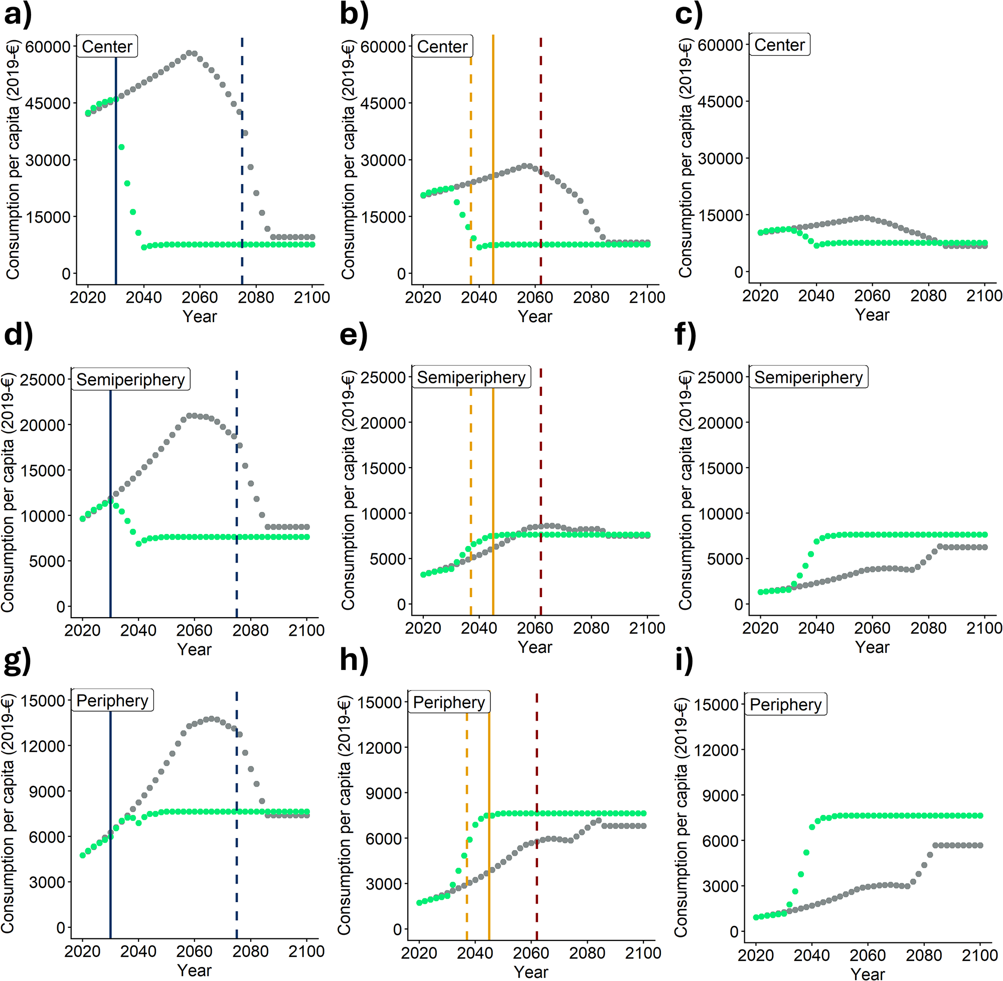
Disaggregating consumption per capita pathways by region and class, we find significant differences between an early- and a late-transition scenario for the majority of classes and during the majority of the simulation time. Consumption pathways are comparable in both scenarios for all classes until redistribution policies are implemented in the early-transition scenario, after which the consumption levels of all classes in the center and the richest class in the semiperiphery decrease strongly, while they continue to grow until approximately 2060 in the late-transition scenario. However, during the last 15 years of the simulation, the consumption levels in these classes converge again due to the implementation of the late-transition social policies (Figure 2a–d). Notably, in the late-transition scenario, the decline of consumption levels for richer classes is driven primarily by emerging limits to growth, with redistribution policies further accelerating the process.
Evolution of annual consumption per capita for the early (green) and late (grey) transition scenario. (a) Richest 20% of the center; (b) middle 50% of the center; (c) poorest 30% of the center; (d) richest 20% of the semiperiphery; (e) middle 50% of the semiperiphery; (f) poorest 30% of the semiperiphery; (g) richest 20% of the periphery; (h) middle 50% of the periphery; and (i) poorest 30% of the periphery. Solid vertical lines refer to the early-transition scenario, whereas dashed vertical lines refer to the late-transition scenario. Blue lines mark the start of the transition, orange lines indicate when the 2°C threshold is crossed, and the red line indicates when the 3°C threshold is crossed.

Figure 2 Long description
A line graph labeled “Center”. The horizontal axis label is “Year” with ticks at 2020, 2040, 2060, 2080, 2100. The vertical axis label is “Consumption per capita (2019-euros)” with ticks at 0, 15000, 30000, 45000, 60000. Two dotted lines are plotted. One dotted line rises from about 45000 at 2020 to about 60000 near 2070, then declines to about 35000 near 2080 and continues down to about 10000 by about 2090, then stays near 10000 to 2100. The other dotted line starts near 45000 at 2020, then drops steeply to about 10000 by about 2040 and stays near 10000 to 2100. One vertical dashed line is drawn near 2080. The image B showing a line graph labeled “Center”. The horizontal axis label is “Year” with ticks at 2020, 2040, 2060, 2080, 2100. The vertical axis label is “Consumption per capita (2019-euros)” with ticks at 0, 15000, 30000, 45000, 60000. Two dotted lines are plotted. One dotted line rises from about 20000 at 2020 to about 28000 near 2060, then declines to about 12000 by about 2090 and stays near 12000 to 2100. The other dotted line starts near 20000 at 2020, drops to about 10000 by about 2040 and stays near 10000 to 2100. Three vertical dashed lines are drawn near 2040, near 2050 and near 2060. The image C showing a line graph labeled “Center”. The horizontal axis label is “Year” with ticks at 2020, 2040, 2060, 2080, 2100. The vertical axis label is “Consumption per capita (2019-euros)” with ticks at 0, 15000, 30000, 45000, 60000. Two dotted lines are plotted. One dotted line stays between about 10000 and about 15000 from 2020 to about 2080, then declines to about 10000 by about 2090 and stays near 10000 to 2100. The other dotted line stays near 10000 from 2020 to 2100. The image D showing a line graph labeled “Semiperiphery”. The horizontal axis label is “Year” with ticks at 2020, 2040, 2060, 2080, 2100. The vertical axis label is “Consumption per capita (2019-euros)” with ticks at 0, 5000, 10000, 15000, 20000, 25000. Two dotted lines are plotted. One dotted line rises from about 10000 at 2020 to about 21000 near 2070, then declines to about 15000 near 2080 and continues down to about 8000 by about 2090, then stays near 8000 to 2100. The other dotted line starts near 10000 at 2020, drops to about 7000 by about 2040, then stays near 8000 to 2100. One vertical dashed line is drawn near 2080. The image E showing a line graph labeled “Semiperiphery”. The horizontal axis label is “Year” with ticks at 2020, 2040, 2060, 2080, 2100. The vertical axis label is “Consumption per capita (2019-euros)” with ticks at 0, 5000, 10000, 15000, 20000, 25000. Two dotted lines are plotted. One dotted line rises from about 3000 at 2020 to about 8000 near 2060, then stays near 8000 to 2100. The other dotted line rises from about 3000 at 2020 to about 7000 by about 2040, then stays near 8000 to 2100. Three vertical dashed lines are drawn near 2040, near 2050 and near 2060. The image F showing a line graph labeled “Semiperiphery”. The horizontal axis label is “Year” with ticks at 2020, 2040, 2060, 2080, 2100. The vertical axis label is “Consumption per capita (2019-euros)” with ticks at 0, 5000, 10000, 15000, 20000, 25000. Two dotted lines are plotted. One dotted line rises from about 0 at 2020 to about 3000 near 2060, then rises to about 5000 near 2080 and stays near 5000 to 2100. The other dotted line rises from about 0 at 2020 to about 6000 by about 2040, then stays near 6000 to 2100. The image G showing a line graph labeled “Periphery”. The horizontal axis label is “Year” with ticks at 2020, 2040, 2060, 2080, 2100. The vertical axis label is “Consumption per capita (2019-euros)” with ticks at 0, 3000, 6000, 9000, 12000, 15000. Two dotted lines are plotted. One dotted line rises from about 6000 at 2020 to about 13000 near 2070, then declines to about 9000 near 2080 and continues down to about 8000 by about 2090, then stays near 8000 to 2100. The other dotted line rises from about 6000 at 2020 to about 8000 by about 2040, then stays near 8000 to 2100. One vertical dashed line is drawn near 2080. The image H showing a line graph labeled “Periphery”. The horizontal axis label is “Year” with ticks at 2020, 2040, 2060, 2080, 2100. The vertical axis label is “Consumption per capita (2019-euros)” with ticks at 0, 3000, 6000, 9000, 12000, 15000. Two dotted lines are plotted. One dotted line rises from about 2000 at 2020 to about 6000 near 2060, then stays near 7000 to 2100. The other dotted line rises from about 2000 at 2020 to about 8000 by about 2040, then stays near 8000 to 2100. Two vertical dashed lines are drawn near 2040 and near 2050. The image I showing a line graph labeled “Periphery”. The horizontal axis label is “Year” with ticks at 2020, 2040, 2060, 2080, 2100. The vertical axis label is “Consumption per capita (2019-euros)” with ticks at 0, 3000, 6000, 9000, 12000, 15000. Two dotted lines are plotted. One dotted line rises from about 1000 at 2020 to about 3000 near 2060, then rises to about 6000 near 2090 and stays near 6000 to 2100. The other dotted line rises from about 1000 at 2020 to about 7000 by about 2040, then stays near 7000 to 2100.
In the case of the richest 20% of the periphery, the early transition causes consumption levels to stabilize around 2040, whereas in the late-transition scenario they continue to grow for more than two decades, reaching a level 1.8 times higher than in the early-transition scenario by 2066 (Figure 2g). At the same time, an early transition accelerates the growth in consumption levels of the poorest 30% of the semiperiphery and the periphery as well as the middle class of the periphery. Conversely, in a late transition consumption levels of these three classes – the poorest 30% of the semiperiphery, the poorest 30% of the periphery, and the middle class of the periphery – begin to stagnate from the 2060s onward, only increase with the onset of the late transition in 2075, and do not reach the levels obtained in the early-transition scenario despite the redistribution policies (Figure 2f, h, and i).
Finally, the consumption levels of the middle class of the semiperiphery follow approximately the same pathways independent from the timing of the transition (Figure 2e).
Thus, an early transition benefits the consumption and living standards of the poorest classes of the semiperiphery and periphery, which, in 2100, constitute more than half of humanity (56% of the world population in FST5, 57% in BAU-GEG). Conversely, a late transition allows the classes of the center and the richest class of the semiperiphery and periphery to grow their consumption during a longer time, thereby maintaining their privileged access to resources. However, by 2100 these classes make up less than a third of the world population in both scenarios.
3.2. Environmental performance
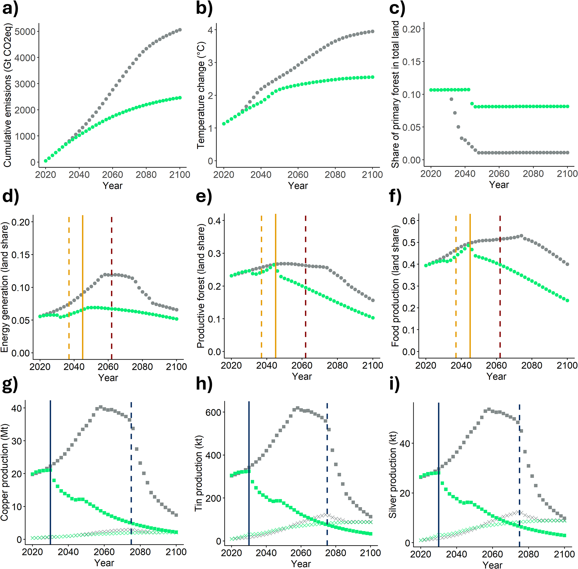
Figure 3 shows a selection of environmental indicators that point to stark differences in the environmental ‘performance’ of a delayed compared to a swift global transition. While cumulative greenhouse gas emissions follow a comparable pathway during the first two decades of the simulation, from 2040 onward, the transition policies in the early-transition scenario strongly curb the increase in emissions. In the late-transition scenario, a slowdown in emissions can be observed from 2080 onward, resulting in cumulative emission levels in 2100 that are more than twice as high as in the early-transition scenario (Figure 3a). This difference is reflected in the projected changes in global average temperatures (Figure 3a). Activated feedbacks in the climate system as well as conservative assumptions about the future evolution of greenhouse gas intensities other than CO2 result in a temperature increase of 2.56°C in 2100 compared to pre-industrial levels, i.e. a failure to reach the 2°C target in the early-transition scenario, despite the strong reductions in overall CO2 emissions. A late-transition scenario, however, not only fails to reach the 2°C climate goal but is linked to a temperature increase of 3.95°C, which is far beyond levels of climate change considered safe (Rockström et al., Reference Rockström, Gupta, Qin, Lade, Abrams, Andersen, Armstrong Mckay, Bai, Bala, Bunn, Ciobanu, DeClerck, Ebi, Gifford, Gordon, Hasan, Kanie, Lenton, Loriani and Zhang2023). Thus, both cumulative emissions and temperature changes indicate that practicing ‘business-as-usual’ beyond the second half of the 21st century will likely push the climate system into high-risk zones and that the timing of the transition might turn out to be crucial for desirable climate outcomes. However, the simulations also indicate that under the boundary conditions chosen for our simulations, even an ambitious transition envisioned to start already in 2030 might turn out to be too late to avoid an ‘overshoot’, i.e. average temperatures more than 2°C higher than the pre-industrial level, during more than half a century. At the same time, although the early-transition scenario might not prevent the activation of several climate tipping points, the late-transition scenario carries a substantially higher risk of pushing the climate system into an irreversible state shift (Armstrong Mckay et al., Reference Armstrong Mckay, Staal, Abrams, Winkelmann, Sakschewski, Loriani, Fetzer, Cornell, Rockström and Lenton2022; Wunderling et al., Reference Wunderling, von der Heydt, Aksenov, Barker, Bastiaansen, Brovkin, Brunetti, Couplet, Kleinen, Lear, Lohmann, Roman-cuesta, Sinet, Swingedouw, Winkelmann, Anand, Barichivich, Bathiany, Baudena and Willeit2024).
Main environmental indicators for the early (green) and late (grey) transition scenario. (a) Cumulative greenhouse gas emissions between 2019 and 2100; (b) global average temperature compared to pre-industrial (1850) levels; (c) share of primary forest in total land; (d) share of land used by the renewable energy sectors in total land; (e) share of economically used forest in total land; (f) share of land used by the food sector in total land; (g) annual copper production for renewable energy technologies (crosses) and for the rest of the economy (squares); (h) annual tin production for renewable energy technologies (crosses) and for the rest of the economy (squares); and (i) annual silver production for renewable energy technologies (crosses) and for the rest of the economy (squares). Solid vertical lines refer to the early-transition scenario, whereas dashed vertical lines refer to the late-transition scenario. Blue lines mark the start of the transition, orange lines indicate when the 2°C threshold is crossed, and the red line indicates when the 3°C threshold is crossed.

Figure 3 Long description
Graph a) shows cumulative greenhouse gas emissions in CO2 equivalent from 2020 to 2100. The x-axis is labeled ‘Year’ and the y-axis ‘Cumulative emissions (Gt CO2eq)’. The early transition scenario (solid line) shows lower emissions compared to the late transition scenario (dashed line), with a significant divergence after 2040. Graph b) illustrates temperature change in degrees Celsius, with the x-axis labeled ‘Year’ and the y-axis ‘Temperature change (°C)’. The early transition scenario results in a lower temperature increase, failing to meet the 2 degrees Celsius target, while the late transition scenario exceeds 3 degrees Celsius. Graph c) depicts the share of primary forest in total land, with the x-axis labeled ‘Year’ and the y-axis ‘Share of primary forest (total share)’. The early transition scenario maintains a higher share compared to the late transition scenario. Graph d) shows the share of land used by renewable energy sectors, with the x-axis labeled ‘Year’ and the y-axis ‘Energy generation (land share)’. The early transition scenario peaks earlier and declines, while the late transition scenario peaks later. Graph e) presents the share of economically used forest in total land, with the x-axis labeled ‘Year’ and the y-axis ‘Productive forest (land share)’. Both scenarios show a peak followed by a decline, with the early transition scenario peaking earlier. Graph f) displays the share of land used by the food sector, with the x-axis labeled ‘Year’ and the y-axis ‘Food production (land share)’. The early transition scenario shows a higher share initially, declining over time. Graph g) illustrates annual copper production in megatons, with the x-axis labeled ‘Year’ and the y-axis ‘Copper production (Mt)’. Crosses represent renewable energy technologies and squares represent the rest of the economy. The early transition scenario shows higher production initially, declining over time. Graph h) shows annual tin production, with the x-axis labeled ‘Year’ and the y-axis ‘Tin production (kt)’. The early transition scenario shows higher production initially, declining over time. Graph i) presents annual silver production, with the x-axis labeled ‘Year’ and the y-axis ‘Silver production (kt)’. The early transition scenario shows higher production initially, declining over time. Solid lines represent the early transition scenario, dashed lines represent the late transition scenario. Blue lines mark the start of the transition, orange lines indicate when the 2 degrees Celsius threshold is crossed and the red line indicates when the 3 degrees Celsius threshold is crossed. Overall, the early transition scenario results in lower emissions, temperature increases and more sustainable land use compared to the late transition scenario.
However, not only climate variables but also other environmental variables evolve differently across the two scenarios. For example, the share of primary forest in total land area (Figure 3c) falls earlier and further in the late-transition scenario – from nearly 11% in 2019 to 1% in 2046 – with only the assumed forest protection policy preventing additional losses. In the early-transition scenario, the loss of primary forest is less pronounced: by 2050, the share of primary forest in total land only has fallen from 11% to 8%, and no further losses occur during the second half of the 21st century. This result is remarkable since land intensity declines faster in the late-transition scenario than in the early-transition scenario. However, the lower levels of output of the food and (non-energy) biomass sector in the early-transition scenario more than offset the higher land intensity.
At the same time, the share of land used for the generation of renewable biomass energy or electricity in total habitable land increases faster in the late-transition scenario and, between 2050 and 2077, is higher than 10%. Only the implementation of transition policies lowers the demand for energy, and thus, the associated land demand. In the early-transition scenario, the maximum share of land used for energy generation is reached in 2049 at 7% and falls slowly afterward to 5% in 2100. Despite the significant decline in land demand, by the end of the simulation, the land share in the late-transition scenario is still 1% higher than in the early-transition scenario (Figure 3d). The land shares of economically used forests (Figure 3e) and of cropland and pastures (Figure 3f) evolve similarly in both scenarios until 2045 despite the implementation of the early-transition policies between 2030 and 2040. During the second half of the 21st century, the variables start to diverge: In the early-transition case, from 2045 onward the share of economically used forest in total land consistently falls, while in the late-transition scenario the variable stabilizes and only begins to fall with the onset of the late-transition policies. In 2100, the share of economically used forest in total land is 55% and 32% below the initial level for the early- and the late-transition scenario, respectively. In both scenarios, the land used by the industrial food sector is projected to occupy almost half of the habitable land by 2045. However, while the early transition in the long term considerably lowers the size of land used for food production, in the late-transition scenario, land used for industrialized agriculture grows to occupy more than 53% in 2075 as both economic growth and land intensity improvements start to reverse in the 2060s.
Although late-transition policies manage to lower the share of land dedicated to food production to the initial level, the long periods of time in which energy and food production claim large shares of the total inhabitable land, coupled with the higher loss of primary forest, imply that the pressure on biodiversity and ecosystem integrity is much higher during the GEG scenario than during the FST5 scenario.
Figure 3g and h shows the projected global production trends of copper, tin, and silver, which serve as essential raw materials for both general industrial applications and renewable energy technologies. In both scenarios, the share of copper, tin, and silver production that is required for renewable energy technologies increases considerably, especially toward the end of the simulation period. Since total metal extraction falls faster in the early-transition scenario while the demand for renewable electricity is comparable in both scenarios, the share of metals dedicated to the renewable energy sector is significantly higher in the early-transition scenario. By the end of the simulation, in the late-transition scenario, half of the tin and silver production is used for the production of renewable energy technologies, the other half being processed by the remaining sectors, while in the early-transition scenario the amount of tin and silver required for renewable energies is significantly higher than the quantity of metals demanded by the rest of the economy. In the case of copper, in the late-transition scenario the rest of the economy still requires 3.45 times more material than the renewable energy sectors, while in the early-transition scenario copper demand of the remaining sectors has decreased to such an extent that half of the total copper production is used for renewable energy technologies.
Comparing the simulation results across multiple environmental indicators, we can detect a trade-off between a reduction of anthropogenic pressure on the environment and a prolonged period of high consumption for richer classes. This trade-off is especially strong in the case of non-renewable stocks and nonlinear tipping points in ecosystems and the climate system. For example, climate tipping points or irreversible state shifts in the Earth’s biosphere (Barnosky et al., Reference Barnosky, Hadly, Bascompte, Berlow, Brown, Fortelius, Getz, Harte, Hastings, Marquet, Martinez, Mooers, Roopnarine, Vermeij, Williams, Gillespie, Kitzes, Marshall, Matzke and Smith2012) could greatly reduce the positive impacts of a late transition on the environment. Likewise, a loss of primary forest and of relatively easily accessible fossil and mineral resources during a time of prolonged ‘business-as-usual’ can no longer be reversed during a delayed transition.
For the poorer classes, a growth-versus-climate trade-off does not seem to apply since in both scenarios, poorer classes see their consumption levels increase during the transition while annual emissions decrease strongly. However, we find a limited trade-off with respect to agricultural land, as rising consumption levels, especially in the case of the poorest classes, in our simulations result in higher demand for agricultural land, and thus, a higher pressure for land conversion.
3.3. Stability assessment
We identify five dimensions that indicate the stability and plausibility of the scenarios toward the end and beyond the 21st century: resource availability, climate change, use of input factors, public and private consumption levels, and mortality rates.
The first three dimensions point to problems in the economic reproduction process: declining resource availability can prevent the economy from fulfilling the desired consumption levels, climate change disturbs economic activities, and if the intensity of input factors increases, the probability of scarcity issues increases. The last two dimensions indicate risks to social reproduction processes: declines in public spending and private consumption levels, as well as increasing mortality rates, might spark social unrest and fuel distribution conflicts.
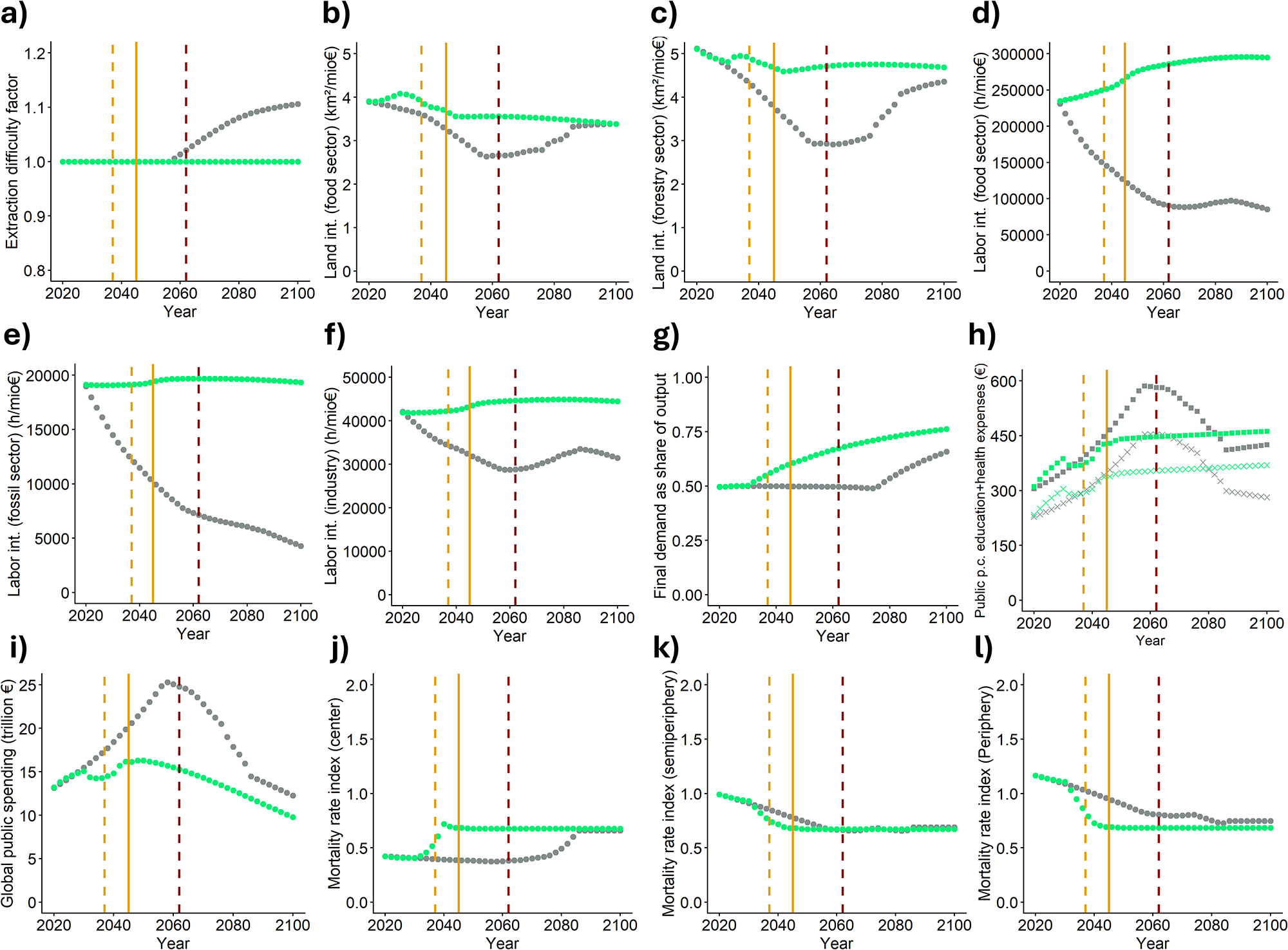
While the early-transition scenario causes fossil fuel extraction to peak in the 2030s, in the late-transition scenario, fossil resource use peaks in 2057 and afterward remains at high levels until the start of the transition. The additional extraction during the BAU phase of the late-transition scenario amounts to more than 19,000 EJ by 2075, almost half of the coal, gas, and oil reserves in the model. Consequently, by 2080, despite the start of the transition, the fossil reserves have been depleted, while in the early-transition case, there are still fossil reserves left by the end of the century. With increasing depletion, resource extraction becomes costlier in terms of input factors required to produce one unit of output in the fossil resource sectors. This is reflected in an increase in the ‘extraction difficulty factor’ (Figure 4a) that grows during the late transition but stays constant in the early transition. Since the higher degree of resource depletion cannot be reversed through transition policies, the late-transition scenario appears less stable in the long term than the early-transition scenario, especially because both scenarios continue to rely on a small but consistent flow of fossil resources that are used, inter alia, as material feedstocks.
Stability indicators for the early (green) and late (grey) transition scenario. (a) Fossil fuel extraction difficulty factor; (b) agricultural land intensity; (c) forest land intensity; (d) labor intensity of the food sector; (e) labor intensity of the fossil energy sector; (f) labor intensity of the industrial sector; (g) final demand as share of output; (h) public per capita education (crosses) and health (squares) expenses; (i) global public spending; (j) mortality rate index in the center; (k) mortality rate index in the semiperiphery; and (l) mortality rate index in the periphery. Solid vertical lines refer to the early-transition scenario, whereas dashed vertical lines refer to the late-transition scenario. Orange (red) lines indicate when the 2°C (3°C) threshold is crossed.

Figure 4 Long description
Twelve line graphs labeled a to l, each showing different stability indicators over time from 2020 to 2100. The horizontal axis is labeled ′Year′. Each graph has a unique vertical axis representing specific metrics. Solid lines indicate early-transition scenarios, while dashed lines indicate late-transition scenarios. Orange and red lines mark when the 2 degrees Celsius and 3 degrees Celsius thresholds are crossed. Graph a: Fossil fuel extraction difficulty factor increases in the late scenario, remains stable in the early scenario. Graph b: Agricultural land intensity shows a slight decrease in both scenarios. Graph c: Forest land intensity decreases more sharply in the late scenario. Graph d: Labor intensity of the food sector decreases in both scenarios, more in the late scenario. Graph e: Labor intensity of the fossil energy sector decreases significantly in the late scenario. Graph f: Labor intensity of the industrial sector decreases in both scenarios. Graph g: Final demand as share of output increases slightly in both scenarios. Graph h: Public per capita education and health expenses increase, with education marked by crosses and health by squares. Graph i: Global public spending increases in both scenarios, more in the late scenario. Graph j: Mortality rate index in the center decreases in both scenarios. Graph k: Mortality rate index in the semiperiphery decreases slightly. Graph l: Mortality rate index in the periphery decreases more in the early scenario. Overall, the early transition scenario generally shows more stability and less drastic changes compared to the late transition scenario.
Another source for long-term instability comes from the accelerated changes in the global climate system produced during the BAU phase of the BAU-GEG scenario (Figure 3b). By the end of the century, the late-transition scenario is projected to face significantly higher levels of climate damages than the early-transition scenario, which exerts permanent pressure on the economic production process. The high-emission pathway before the transition risks triggering critical thresholds in the climate system, such as an irreversible decline of the northern AMOC (Drijfhout et al., Reference Drijfhout, Angevaare, Mecking, van Westen and Rahmstorf2025), which can lead to additional, permanent damages to the economy that are not represented by the model.
Last, comparing different intensity parameters of the two scenarios (Figure 4b–f), we find some interesting dynamics. First, during the BAU phase of the late transition scenario, the improvement in different land and labor intensity parameters slows down and reverses. This change in the long-term trend can be interpreted as a sign of rising instability of the scenario. The implementation of transition policies, however, manages to slow down the increase in land intensities. Due to the exogenous labor intensity component in the model, labor intensities eventually even begin to fall again, despite ongoing climate damages negatively affecting labor productivities. Thus, the late transition yields at least some temporal stability to the BAU-GEG scenario.
Due to different boundary conditions, land and labor intensities in the early-transition scenario are consistently higher than in the late-transition scenario. However, unlike in the late-transition scenario, the long-term trend in land productivities is positive. The impact of climate damages can be clearly seen through rising labor intensities in different sectors. The ratio between labor demand and labor supply is high but stable throughout the scenario. Thus, interestingly, despite the losses in productivity due to climate damages and the loss of labor supply due to a strong decrease and aging of the world population, there is no sign of an emergent labor scarcity issue in the early-transition scenario.
An additional variable linked to the use of input factors is the ratio between final demand and total output (Figure 4g). The decline in this ratio before the application of strong sustainability policies can be considered a sign of increasing instability as a greater part of economic activity is dedicated to satisfying industry demand through the production of intermediate goods, rather than final demand. The transition exerts a positive effect by increasing the value of this variable under both scenarios; however, the final value attained is comparatively higher in the case of an early transition.
Turning to the potential risks for social reproduction processes, we find that by the end of the simulation, projected per capita levels are at a comparable low level in both scenarios, with a slightly higher consumption of the poorest classes in the early-transition scenario. Although global public consumption is higher in the late-transition scenario (Figure 4i), public per capita expenditures for health and education after the transition are lower than in the early-transition scenario (Figure 4h), given that the storyline of this scenario foresees higher public expenses for security. Consequently, the key stability risk in the late-transition scenario arises less from low overall consumption than from the sharper declines affecting central regions and the richest classes elsewhere. Since these groups experience prolonged growth before the downturn, their perceived losses are greater than in the early-transition scenario, increasing the likelihood of social tensions. In general, the extreme rapidity and intensity of changes in consumption levels in both scenarios could cause massive social tension if implemented without broad support among the world population. This widespread consensus about the need to transition to an egalitarian frugal society is postulated in both storylines and driven by ideological changes in the case of the early transition, and by increasing experiences of negative impacts from environmental destabilization in the case of the late transition scenario. Although the scenarios do not specify the concrete form the global redistribution policies might take, arguably a combination of policies including resource caps, public production of essential goods, strategic investment in the periphery, and global capital distribution will be necessary to drive the transition process. A social transition process over a 20-year period instead of the modeled ‘extreme case’ of 10 years might increase social feasibility but also would lead to further environmental degradation and crossing of planetary boundaries.
Finally, the changes in mortality rates caused by transition policies are comparable in both scenarios, and benefit the semiperiphery and periphery. Thus, there is a certain trade-off between the evolution of the mortality rates in the three world regions: In an early-transition scenario, the center sees its mortality rate increase early in time, due to a strong decrease in consumption, while the periphery’s mortality rates fall significantly. In the late-transition scenario, the mortality rates of the center stay low during most of the simulation period, while the mortality rates of the other world regions decline at a lower rate than in the early-transition scenario. The mortality index depicted in Figure 4j and k is calculated to take a value of 1 for the initial mortality rate in the semiperiphery for people aged 45–49, and approaches 0.7 in both scenarios and in all world regions by the end of the simulation. Thus, despite the loss of life expectancy in the center, the early- as well as the late-transition policies can prevent the risks of an excessive increase in mortality rates in poorer regions due to emerging limits to growth.
In conclusion, while a late transition might be capable of temporarily increasing the world system’s stability and preventing undesirable dynamics of accelerated economic breakdown, an early transition is linked to higher stability in the longer term.
4. Discussion
As with every other modeling study, it is important to interpret our results in the context of the model used and the assumptions made. Thus, in the following, we highlight several key scenario assumptions that influence the quantitative simulation results presented in the previous section.
First, in both the early and the delayed transition scenarios, we assume relatively fast rates of social and political change that can even surpass the rates of technological change. For example, in the GEG scenario, major social changes occur within 10 years, while technological changes take 50 years to reach the scenario targets. This sets our scenario analysis apart from modeling studies that project fast improvement rates in energy and CO₂ intensity while excluding fast structural change in the social realm (Grandjean et al., Reference Grandjean, Lepetit and Morel2019). Although various theories of socio-technological change have attempted to formalize the nonlinear dynamics occurring under sustainability transitions (Petrović, Reference Petrović2023), maximum future rates of change in critical variables remain highly uncertain.
Second, although fertility rates do not necessarily fall faster during the transition period than historical declines in fertility rates between 1950 and 2020, the consistent application of a population policy exerting a downward pressure on birth rates over time, in addition to consumption- and education-induced declines in fertility rates, leads to a strong degrowth in world population in both scenarios. Although, ceteris paribus, this trend reduces environmental pressure, an aging population and a reduction in the labor force could give rise to a series of socioeconomic changes and risks not accounted for in the simulations such as declines in labor productivity growth (Esposito, Reference Esposito2025; Maestas et al., Reference Maestas, Mullen and Powell2023), declines in interest rates (Bielecki et al., Reference Bielecki, Brzoza‐brzezina and Kolasa2023) and demography-related changes in inflation (Mazumder & Diwakar, Reference Mazumder and Diwakar2025a, Reference Mazumder and Diwakar2025b).
Third, our scenario assumptions reflect a certain optimism bias (Korteling & Toet, Reference Korteling and Toet2022), i.e. a possible overestimation of technological progress combined with a possible underestimation of environmental damages: On the one hand, we simulate a range of positive technological changes, such as an economy-wide shift from fossil to bioenergy, and considerable efficiency improvements due to product reuse and material recycling. On the other hand, the climate damage factors used for the simulations do not consider high-impact events with low or unknown probability, which would arguably lead to more severe disruptions of economic and governance processes. Regarding ecosystem properties, our scenarios are consistent with the assumption of highly resilient ecosystems, while they would likely cease to be feasible under brittle ecosystems (Cumming et al., Reference Cumming, Alcamo, Sala, Swart, Bennett and Zurek2005).
Last, the assumed decrease in land, labor, and energy intensities due to learning and technological progress that takes place over time could, in theory, render an early transition less efficient than a late transition. However, in our simulations this trade-off does not manifest, since the reduction in overall economic activity is large enough to make a successful transition feasible even with higher intensities.
Despite these caveats, our work makes relevant contributions to the literature on sustainability transitions. Generally, our simulations support previous findings in the literature that early transitions are preferable to late transitions from an environmental and economic perspective. Various studies have shown that an earlier adaptation of mitigation measures positively influences total mitigation costs and decarbonization pathways of the energy system (Sanderson & O'Neill, Reference Sanderson and O'Neill2020; Victoria et al., Reference Victoria, Zhu, Brown, Andresen and Greiner2020), reduces carbon lock-in and the risks of stranded assets (Fisch-Romito et al., Reference Fisch-Romito, Guivarch, Creutzig, Minx and Callaghan2021; Mercure et al., Reference Mercure, Pollitt, Viñuales, Edwards, Holden, Chewpreecha, Salas, Sognnaes, Lam and Knobloch2018), and leads to lower economic damages (Burke et al., Reference Burke, Alampay Davis and Diffenbaugh2018). Similarly, our simulation results point to significantly lower economic losses and improved environmental outcomes when society takes action relatively early. However, due to our methodologically different modeling approach, we obtain benefits regarding an earlier transition that transcend considerations of cost-effectiveness: our simulations explore different timings of social policies and their effects on the poorest and most vulnerable population groups as well as on macroeconomic system stability. Thereby, our work helps to address the relative lack of simulations of strong social policies, including post-growth, sufficiency, and redistribution policies in IAMs. By comparing early and delayed social action alongside technological changes, we show that time lags in societal reactions to environmental problems have significant high-level effects on dynamically changing global social, economic, and ecological systems. To the best of our knowledge, this paper is the first to quantitatively explore the link between time-lag analyses (Hocherman et al., Reference Hocherman, Trop and Ghermandi2025) and the study of post-growth (Kallis et al., Reference Kallis, Hickel, O'Neill, Jackson, Victor, Raworth, Schor, Steinberger and Ürge-Vorsatz2025).
Our simulations enrich and deepen the selected qualitative storylines by demonstrating that narrative descriptions of key patterns can be replicated through quantitative modeling. Focusing on the factor of time in radical just sustainability transitions, we show that an early transition is clearly desirable in terms of system stability, consumption of poorer classes, and environmental outcomes. However, while our findings support the urgency of just transitions, they also illustrate that it is never ‘too late’ for ambitious social, ecological, and economic policies. Thus, even when emerging limiting factors begin to affect the global accumulation regime, there remain policy options to avoid worst-case socio-ecological outcomes. The existence of time lags in societal responses to environmental problems unfolding over long time scales, by itself, does not justify fatalistic accounts of humanity’s future. Nevertheless, our simulations also point to the framework conditions necessary to achieve strong climate mitigation and avoid a massive surge in mortality rates among poorer classes – namely, a declining world population size, ambitious technological policies, and extremely fast and strong convergence and reductions in consumption. Based on our simulations, we hypothesize that the later the transition occurs, the higher the probability that it will take on a ‘radical’ post-growth character, since the adverse impacts of a destabilized Earth system on productive capacities increase the need for redistribution and equitable resource access to prevent the exclusion of an ever greater part of the world population from access to basic economic goods.
Consequently, we propose that future research further explore sustainability transitions occurring under non-ideal circumstances, including delays, maladaptation, adoption of non-optimal technological options, insufficient social redistribution, and planning failures. Quantifying such scenarios could provide society and policymakers with more realistic assessments of the socio-environmental outcomes that can be expected of future societal transitions and inform the design of policies aimed at enhancing system resilience and minimizing catastrophic harm to vulnerable human populations.
5. Conclusion
In this paper, we examined how the timing of a global ‘just sustainability transition’ shapes socioeconomic and ecological outcomes using a comparative scenario analysis with the MORDRED-IAM. Our findings show that an early transition can prevent unintentional economic degrowth caused by environmental degradation, while achieving social consumption and redistribution targets through slower rates of change. In contrast, a delayed transition implies that the consumption declines among wealthier groups are driven first by emerging biophysical limits and later intensified by redistribution policies. Both pathways involve trade-offs – most notably between sustaining higher consumption levels and breaching critical ecological thresholds. Although a delayed transition may temporarily stabilize the global system and avoid a catastrophic economic breakdown, an earlier start of radical post-growth policies yields greater long-term resilience. Our results underscore the importance of modeling sustainability transitions under non-ideal conditions and indicate the important role radical post-growth policies could play in societal transitions that occur relatively late and in the context of mounting environmental pressures.
Supplementary material
The supplementary material for this article can be found at https://doi.org/10.1017/sus.2026.10076.
Acknowledgements
N/A.
Author contributions
A.H.L.: Conceptualization, Data curation, Formal analysis, Methodology, Software, Visualization, Writing – original draft, Writing – review & editing. L.L.: Conceptualization, Software, Writing – review & editing.
Data availability statement
Data will be made available on request.
Funding statement
No financial support was received.
Competing interests
The authors report no potential conflict of interest.


 Open access

