2. Numerical set-up

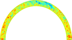
We have carried out four DNSs of fully developed turbulent flows in mildly to strongly curved channels. The incompressible Navier–Stokes equations in cylindrical coordinates are solved in a domain bounded by sectors of two concentric cylinders, as in Moser & Moin (Reference Moser and Moin1987), see figure 1 for an illustration of the computational domain. Streamline curvature effects on turbulent flow in curved channels as in figure 1 are similar to rotation effects on turbulent plane channel flows subject to clockwise rotation about the spanwise axis. Fourier representations with periodic boundary conditions are used in the homogeneous streamwise (azimuthal) and spanwise (axial) directions and a sixth-order compact-finite-difference scheme is used in the wall-normal (radial) direction with no-slip conditions at the walls (Boersma Reference Boersma2011; Peeters et al. Reference Peeters, Pecnik, Rohde, van der Hagen and Boersma2016). The solution is advanced by a pressure correction method together with a fourth-order Runge–Kutta method for time integration. The Poisson equation for the pressure is solved directly using Fourier transforms in the streamwise and spanwise directions and LU factorization of the matrix resulting from the discrete Poisson equation in the radial direction. The computational domain has a streamwise length of $12{\rm \pi} \delta$ along the centreline and a spanwise width of $3{\rm \pi} \delta$, which is equally wide but 1.5 times longer than in recent DNS of plane channel flow (Lee & Moser Reference Lee and Moser2015) to accommodate the long structures, and three times longer and more than two times wider than in the DNS by Moser & Moin (Reference Moser and Moin1987). In the DNS with strongest curvature the domain captures an entire cylinder circumference.

Figure 1.

Illustration of the computational domain for curved channel flow. The wall-normal direction $y$ is from the convex (inner) wall towards the concave (outer) wall.

The bulk Reynolds number $Re=U_b \delta /\nu$ is fixed at $20\,000$ by enforcing a constant mass flow rate, giving a $Re_\tau = u_\tau \delta /\nu$ of approximately 1000. Here, $U_b$ is the bulk mean velocity, $u_\tau$ friction velocity defined later and $\nu$ viscosity. The number of grid points, resolution, curvature and friction Reynolds numbers together with the reference names of the four DNSs are listed in table 1. From now on, curvature refers to $\gamma = 2\delta /r_c$, where $r_c$ is again the curvature radius at the channel centreline. Run R0 is a DNS of plane channel flow at the same $Re$ with a domain $8{\rm \pi} \delta$ long and $3{\rm \pi} \delta$ wide, taken from Brethouwer (Reference Brethouwer2017). Here, $Re^i_\tau$ and $Re^o_\tau$ are the friction Reynolds numbers based on the friction velocities $u_{\tau i}$ and $u_{\tau o}$ for the inner and outer walls, respectively.

Table 1.

Run name, channel curvature, friction Reynolds numbers and number of streamwise, wall-normal and spanwise grid points $N_x$, $N_y$, $N_z$, respectively.

The streamwise and spanwise resolutions in all DNSs are $r\Delta \theta ^+ \leq 13$ and $\Delta z^+ \leq 6.5$, respectively, in viscous wall units and Fourier modes, comparable to the resolutions used by Lee & Moser (Reference Lee and Moser2015). The resolution is coarsest near the outer wall since, there, the friction velocity is higher and the domain longer. Grid points in the radial direction are clustered near the wall with at least 7 grid points in the viscous sublayer $y^+ \leq 5$ and the first grid point at $y^+ < 0.5$. Some validations of the numerical methodology are presented in Appendix A.

The balance between mean streamwise pressure gradient $\textrm {d} P /(r_c \,\textrm {d} \theta$), the total mean wall shear stress $\tau _{tot}$ and friction velocities is given by

(2.1)\begin{equation} u^2_\tau = \frac{\tau_{tot}}{\rho} ={-}\frac{\delta}{\rho r_c} \frac{\textrm{d} P}{\textrm{d} \theta} = \frac{r^2_i u^2_{\tau i} + r^2_o u^2_{\tau o}}{2 r^2_c} , \end{equation}

where $r_i$ and $r_o$ is the inner and outer wall radius, respectively, P the mean pressure and $\rho$ the density. The total mean shear stress obeys

(2.2)\begin{equation} \bar{\tau}=\nu \left( \frac{\partial U}{\partial r}-\frac{U}{r}\right) - \overline{uv} = \frac{1}{4 r^2 r_c\delta} [ r^2_i (r^2_o - r^2)u^2_{\tau i} + r^2_o (r^2_i - r^2)u^2_{\tau o}], \end{equation}

where $U$ is the mean streamwise velocity, $u$ and $v$ streamwise and wall-normal velocity fluctuations and an overline implies averaging in time and homogeneous azimuthal and axial directions. The derivation is given in Appendix B.

The DNSs are run for a sufficiently long time to reach a statistically stationary state and then run for at least $280 \delta /U_b$ to obtain well-converged statistics.

3. Flow statistics

First, mean flow, wall shear stress and turbulent fluctuation statistics are presented. In the next sections, Reynolds-stress budgets and flow structures are studied. In the following figures $y=(r-r_c)/\delta$, with $y=-1$ and 1 at the inner (convex) and outer (concave) wall, respectively. Many figures include results of plane channel flow case R0. Similarities between the present curved channel flow cases and plane channel flow rotating about the spanwise axis are expected, as noted in the Introduction, and also further discussed. The mean streamline turning rate is $U/r$ in curved channel flow, with $U$ the mean streamwise velocity. This suggests replacing the rotation rate $\varOmega$ in the rotation number $Ro=2\varOmega \delta /U_b$ of spanwise rotating channel flow by $U_b/r_c$ to obtain that an equivalent rotation number for curved channel flow of $Ro=2\delta /r_c=\gamma$. Thus, it appears meaningful to compare rotating and curved channel flows for $Ro=\gamma$ when rotation and curvature effects are comparable. In Brethouwer (Reference Brethouwer2017), results of spanwise rotating channel flow DNS at $Re=20\,000$ are reported, but only one case with $Ro=0.15$ has a $Ro$ that falls into the range of curvatures $\gamma \simeq Ro \leq 0.333$ considered here. The other cases have $Ro \geq 0.45$, corresponding to much stronger curvatures. Results of the rotating channel flow DNS at $Re=20\,000$ and $Ro=0.15$ are included in some figures to make a few comparisons possible.

Figure 2(a) shows mean streamwise velocity profiles $U/U_b$ in the curved channel flow DNSs. The mean shear is remarkably weak for $0 \lesssim y \lesssim 0.6$ and the velocity gradient is even slightly positive at the centreline in the mild curvature cases R1 and R2 but the profiles become more oblique for increasing curvature. This is owing to the development of a core region in runs R1 to R4 with a nearly constant mean specific angular momentum $rU$, see figure 2(b), as observed in previous experiments of strongly curved duct flows with $r_c/\delta \leq 19$ (Wattendorf Reference Wattendorf1935; Eskinazi & Yeh Reference Eskinazi and Yeh1956). Here, we see that an irrotational mean flow region tends to emerge for $r_c/\delta \leq 30$, skewed towards the outer concave side and expanding with increasing curvature. Fluid elements thus tend to preserve angular momentum when being displaced by eddies in the radial direction. A core region with nearly constant angular momentum also develops in turbulent Taylor–Couette flows and implies a trend towards neutral stability according to Rayleigh's inviscid criterion for centrifugal instability (Brauckmann et al. Reference Brauckmann, Salewski and Eckhardt2016). A similar phenomenon occurs in spanwise rotating plane Couette and channel flow, in which a neutrally stable zero-absolute-mean-vorticity region emerges (Brauckmann et al. Reference Brauckmann, Salewski and Eckhardt2016; Brethouwer Reference Brethouwer2017). Constant angular momentum furthermore implies that the total production of streamwise Reynolds stress $\overline {uu}$ given by $P_{uu} = -2 \overline {uv} (r \partial (U/r)/\partial r + 2 U/r)$ (Hunt & Joubert Reference Hunt and Joubert1979) becomes zero. Here, the first term on the right-hand side is the shear production term and the second term an additional production term owing the curvature strain. This additional production term $4\overline {uv}U/r$ is present as well in the wall-normal Reynolds-stress $\overline {vv}$ transport equation, although with an opposite sign. It can be seen as a redistribution term between the normal Reynolds stresses since it influences turbulence anisotropy, as we see later, but it is absent in the turbulent kinetic energy transport equation (Hunt & Joubert Reference Hunt and Joubert1979). In the mild curvature cases a small extra production term due to curvature is still able to offset the shear production term in $P_{uu}$ because the mean shear is very weak, as shown in figure 2(a). The shear production and additional production owing to curvature are studied in the next section. Again, similarities with spanwise rotating shear flows show up: the Coriolis term redistributes energy between the normal Reynolds stresses but does not directly contribute to turbulent kinetic energy. Furthermore, the sum of shear production and Coriolis term in the $\overline {uu}$ transport equation becomes zero in the zero-absolute-mean-vorticity state (Brethouwer Reference Brethouwer2017).

Figure 2.

Profiles of the (a) normalized mean streamwise velocity $U/U_b$ and (b) specific angular momentum $rU$ scaled by its maximum value. Panels (c) and (d) show $U^*$ as functions of $y^*$ on the convex (inner) and concave (outer) channel side, respectively.

Figure 2(c,d) shows the mean streamwise velocity $U^*$ on the inner and outer channel side, respectively, as functions of wall distance $y^*$ in local scaling. Local scaling, denoted by a superscript $*$, implies scaling based on the local friction velocity $u_{\tau i}$ and $u_{\tau o}$ at the inner and outer channel wall, respectively. The curved channel profiles away from the wall lie above and below the plane channel flow profile on the convex and concave sides as a result of the reduced and enhanced turbulent shear stresses, respectively (Moser & Moin Reference Moser and Moin1987), and depart earlier from the R0 profile for stronger curvature. On the concave side all profiles approximately collapse for $y^* \lesssim 50$ but on the convex side the R3 and R4 profiles diverge at smaller $y^*$, indicating that strong curvature affects the flow even near the walls. An identifiable log layer is thus absent in these mildly to strongly curved channels. At a given $y^+$ in the log layer the curvature related production to shear production ratio $(U/r)/(\partial U/\partial r) \sim \delta /(Re_\tau r_c)$. The log layer therefore likely reappears at higher $Re_\tau$ when the boundary layer becomes thinner and shear production grows relative to curvature related production near the wall. Hunt & Joubert (Reference Hunt and Joubert1979) observed a log-layer profile on both sides in experiments with $Re_\tau \approx 700$ to 2700, but their channel was only weakly curved with $r_c/\delta =200$.

Figure 3(a) shows computed total mean shear stress $\bar {\tau }$ profiles, i.e. the sum of viscous and turbulent shear stresses, scaled by $\tau _{tot}$ defined in (2.1). The profiles show the expected growth and decline of shear stress magnitude on the convex and concave side, respectively, and collapse on the derived profile given by (2.2), implying that the statistics are well converged. The mean wall shear stresses $\tau _w$ on the inner and outer walls, shown in figure 3(b), deviate significantly from that of the plane channel flow case R0 already for the weakest curvature considered. For curvatures larger than in case R2, $\tau _w$ does not grow much more and actually starts to decline on the concave side whereas on the convex side $\tau _w$ declines monotonically with curvature owing to a continuing weakening of turbulence. The total mean wall shear stress $\tau _{tot}$ and related flow resistance in the present curved channel flows, on the other hand, are only moderately higher than in plane channel flow, consistent with observations by Wattendorf (Reference Wattendorf1935). Data of spanwise rotating channel flow DNS at $Re=20\,000$ and $Ro=0.15$ (Brethouwer Reference Brethouwer2017) are also included in figure 3(b). Figure 3(b) indicates that, at least for moderate $Ro$, the effects of rotation and curvature on mean wall shear stresses are comparable.

Figure 3.

(a) Total mean shear stress $\bar {\tau }$ profiles scaled by $\tau _{tot}$. Thin solid lines are DNS data and thick dashed lines show $\bar {\tau }$ given by (2.2). (b) Mean wall shear stresses $\tau _w$ on the inner (green) and outer walls (red) and $\tau _{tot}$ (blue) scaled by the mean wall shear stress $\tau _0$ in plane channel flow (run R0). Each dot represents a DNS. The triangles are corresponding rotating channel flow data at the same $Re$ and $Ro=0.15$.

Root-mean-square profiles of all velocity fluctuation components and Reynolds shear stresses in global scaling, i.e. scaled by $u_\tau$, are shown in figure 4. In the convex near-wall region the velocity fluctuations monotonically decline with curvature, concurrently with the mean wall shear stress, whereas the near-wall peak of the streamwise and wall-normal fluctuations does not vary much with curvature on the concave side. On the other hand, spanwise and especially wall-normal fluctuations drastically grow and streamwise fluctuations decline in the outer concave region for strong curvatures. This growth and decline can be explained by the action of the extra curvature production term, which transfers energy from streamwise to wall-normal fluctuations, as discussed before. Energy transfer between the velocity components due to the extra curvature production is studied in the next section and shown to be relatively small in the near-wall region but significant in the outer region. The growth of wall-normal and spanwise fluctuations comes along with a structural change of turbulence and amplification of large-scale structures on the concave side, as shown later.

Figure 4.

Root-mean-square profiles of (a) streamwise, (b) wall-normal and (c) spanwise velocity fluctuations and (d) profiles of the mean turbulent shear stress $\overline {uv}$ in global scaling.

In local scaling, by contrast, streamwise and wall-normal velocity fluctuations are very similar in the convex and concave near-wall region for different curvatures, see figure 5(a,b), suggesting that the near-wall dynamics is mostly unaffected by wall curvature. On the convex side the similarity to plane channel flow extends quite far, up to $y^* \approx 200$. On the concave side the similarity ends earlier because profiles of the strongly curved cases diverge beyond the buffer layer. In run R4 the near-wall peak of the wall-normal component disappears as a result of the strong growth of the fluctuations in the outer region caused by a fundamental change in the outer layer dynamics. Near-wall similarity, also observed in experiments of a turbulent boundary layer on a concave wall by Barlow & Johnston (Reference Barlow and Johnston1988) and in DNS by Moser & Moin (Reference Moser and Moin1987), is to be expected since the strain-rate ratio $(U/r)/(\textrm {d} U/\textrm {d} r)$ decreases and thus curvature effects vanish approaching the wall. Curvature effects on the Reynolds stress budgets are accordingly small to moderate in the near-wall region, as shown in the next section, which further supports the expectation that velocity fluctuations display near-wall similarity in local scaling. The present results suggest that turbulence models and wall-modelled large-eddy simulations (Bose & Park Reference Bose and Park2018) do not have to take into account curvature effects on turbulence in the near-wall region up to quite strong curvatures and that changes in the wall shear stresses are driven by changes in the turbulence dynamics further away from the walls.

Figure 5.

Root-mean-square profiles of the (a) streamwise and (b) wall-normal velocity fluctuations and (c) correlation coefficient $\rho$ on the convex (dashed lines) and concave sides (solid lines) in local scaling. Included in (a,b) are profiles in local scaling (labelled as ‘rot’) from DNS of spanwise rotating channel flow at $Re=20\,000$ and $Ro=0.15$ (Brethouwer Reference Brethouwer2017) on the cyclonic (dashed line) and anticyclonic sides (solid line).

Figure 5(a,b) also includes local scaling profiles of streamwise and wall-normal fluctuations in rotating channel flow DNS at $Re=20\,000$ and $Ro=0.15$ on the cyclonic and anticyclonic channel sides. Although rotation and curvature effects differ in the near-wall regions (note that the mean streamline turning rate varies as $U/r$ and vanishes approaching the wall whereas $\varOmega$ is constant), the profiles basically collapse, implying that rotation and curvature effects are similar and less significant in the near-wall region at least up to $Ro=0.15$. However, stronger rotation with $Ro\geq 0.45$ starts to affect near-wall turbulence (Brethouwer Reference Brethouwer2017), indicating that also stronger curvatures could start to influence near-wall turbulence.

Nagata & Kasagi (Reference Nagata and Kasagi2004), however, did not observe near-wall similarity in their DNSs of curved channel flow; the profiles on the convex and concave sides and for different curvatures showed substantial differences in local scaling, although that was possibly a consequence of a low $Re_\tau =150$. In the present DNSs, near-wall similarity also holds less well for the correlation coefficient $\rho = |\overline {uv}|/(\overline {uu}\,\overline {vv})^{1/2}$ on the convex side in the strongly curved cases (figure 5c), which may explain the early departure of the mean velocity profiles in R3 and R4 seen in figure 2(c). The figure further shows that $u$ and $v$ fluctuations are highly correlated in the outer layer of the concave side in R1 to R4, contributing to the high shear stresses on the concave side. This high correlation points to the presence of coherent turbulent structures.

4. Reynolds-stress budgets

To obtain further insights into the effect of curvature on the turbulence, we consider in this section the budget terms of the Reynolds-stress equations. Budgets at lower $Re_\tau$ have been studied by Moser & Moin (Reference Moser and Moin1987) for a mildly curved channel. The streamwise and wall-normal components of the non-dimensional Reynold-stress equations for the present case read, respectively (Hunt & Joubert Reference Hunt and Joubert1979; Moser & Moin Reference Moser and Moin1987)

(4.1)\begin{align} \frac{\partial \overline{u^2}}{\partial t} &={-}2 \overline{uv} r \frac{\partial U/r}{\partial r} -4 \overline{uv} \frac{U}{r} -2 \overline{\frac{u}{r}\frac{\partial p}{\partial \theta}} -\frac{1}{r} \left ( \frac{\partial r \overline{vu^2}}{\partial r} + 2 \overline{vu^2} \right )\nonumber\\ &\quad +\frac{1}{Re} \left ( \frac{1}{r} \frac{\partial}{\partial r} r \frac{\partial \overline{u^2}}{\partial r} + 2 \frac{\overline{v^2}-\overline{u^2}}{r^2} \right )\nonumber\\ &\quad -\frac{2}{Re} \left (\overline{\left ( \frac{\partial u}{\partial r} \right )^2}+ \overline{\left ( \frac{\partial u}{\partial z} \right )^2}+ \frac{1}{r^2}\overline{\left ( \frac{\partial u}{\partial \theta} + v \right )^2} \right), \end{align}

(4.2)\begin{align} \frac{\partial \overline{v^2}}{\partial t} &= 0 + 4 \overline{uv} \frac{U}{r} -2 \overline{v\frac{\partial p}{\partial r}} -\frac{1}{r} \left ( \frac{\partial r \overline{v^3}}{\partial r} - 2 \overline{vu^2} \right )\nonumber\\ &\quad +\frac{1}{Re} \left ( \frac{1}{r} \frac{\partial}{\partial r} r \frac{\partial \overline{v^2}}{\partial r} - 2 \frac{\overline{v^2}-\overline{u^2}}{r^2} \right )\nonumber\\ &\quad -\frac{2}{Re} \left ( \overline{\left ( \frac{\partial v}{\partial r} \right )^2}+ \overline{\left ( \frac{\partial v}{\partial z} \right )^2}+ \frac{1}{r^2}\overline{\left ( \frac{\partial v}{\partial \theta} - u \right )^2} \right). \end{align}

Here, $p$ is the pressure fluctuation. On the right-hand side of these equations, the terms represent shear production, an additional production resulting from curvature, velocity–pressure gradient, turbulent diffusion, viscous diffusion and dissipation, respectively. The shear production term in the equation for $\overline {vv}$ is naturally zero.

Figure 6 shows the budgets of (4.1) and (4.2) in local wall unit scaling near the convex and concave walls in R3. The budgets in R0 are also shown for comparison to elucidate the curvature effect. Only small differences exist in the budgets of $\overline {uu}$ in R0 and R3 on the convex and concave sides and the additional production term in R3 is negligible near the walls. The additional production term is, however, noticeable in the balance equation of $\overline {vv}$, as seen in figure 6(c,d). On the concave side it is positive and produces wall-normal Reynolds stresses while on the convex side it reduces them owing to the different sign of $\overline {uv}$. Concave curvature leads to a moderate reduction of the velocity–pressure gradient and dissipation term and augmentation of turbulent diffusion of $\overline {vv}$ while convex curvature has the opposite effect. Similar curvature effects are seen in the other runs and not shown here. To summarize, curvature effects on the Reynolds-stress budgets are small to quite moderate in the near-wall regions.

Figure 6.

Budgets of the streamwise Reynolds-stress equation (4.1) on the (a) convex and (b) concave sides and budgets of the wall-normal Reynolds-stress equation (4.2) on the (c) convex and (d) concave sides in local wall units. Solid lines: case R3, dashed lines: case R0.

Figure 7 shows the budgets of (4.1) and (4.2) in R0, R3 and R4 in global wall unit scaling with $u_\tau$. The focus is here on the core region, where curvature effects are most prominent. Viscous diffusion is not shown since it only contributes in the viscous sublayer and buffer layer, see figure 6. The additional production term $\pm 4\overline {uv}U/r$ resulting from curvature is significant in R3 and R4 and to a lesser extent in R1 and R2 (not shown here) and basically offsets the shear production of $\overline {uu}$ on the concave side until $y \approx -0.3$ to -0.4. The underlying reason is the development of an irrotational mean flow region in curved channel flow DNSs, which implies that the total production, i.e. the sum of shear and additional productions, of $\overline {uu}$ becomes zero and the shear production contribution is basically transferred to the $\overline {vv}$-stress component, as discussed before, see figure 7(d,f). The velocity–pressure gradient term in the balance equation of $\overline {uu}$ is negative in R0 but becomes positive in the core region for strong curvatures and contributes to streamwise stresses. In the balance equation of $\overline {vv}$ this term is positive or nearly zero around the centre in R0 but becomes negative in the core region in R3 and R4. In addition, the magnitude of turbulent diffusion of $\overline {uu}$ and $\overline {vv}$ in the core region grows with curvature. This growth is presumably caused by coherent large-scale motions, which are studied in the next section. Turbulent diffusive transport of kinetic energy by large-scale motions presumably contributes to the strong turbulence in the core region even when, as in R1 and R2, mean shear (figure 2a) and accordingly shear production are small. It can be further noticed that the additional production term owing to curvature is negative for $\overline {vv}$ and positive for $\overline {uu}$ on the convex side in R3 and R4 and, consequently, transfers energy from wall-normal to streamwise stresses.

Figure 7.

Budgets of the (a,c,e) streamwise Reynolds-stress equation (4.1) and (b,d,f) wall-normal Reynolds-stress equation (4.2) in global wall units; (a,b) R0, (c,d) R3 and (e,f) R4.

5. Large-scale structures

Large-scale structures develop in curved channel flows but their characteristics and importance for different curvatures remain elusive. In this section, we therefore study turbulence structures and specifically the large ones as well as their contribution to the Reynolds stresses.

Figure 8 shows visualizations of instantaneous flow fields in planes at a constant radius, i.e. at a constant wall distance. Flow field visualizations of case R0 and rotating channel flow are added for comparison. On the convex side no large-scale structures are visible in R4 (figure 8a) and the other curved channel cases (not shown here). In R4 the curvature is strong enough to cause local flow relaminarization near the convex wall since laminar-like patches without small-scale turbulence develop (figure 8a), similar to rotating channel flow where the flow relaminarizes on the cyclonic side at sufficiently high rotation rates. This indicates that curvatures as strong as in R4 and stronger start to affect the near-wall dynamics on the convex side at this $Re$. No large-scale structures are seen in the wall-normal flow field in the outer layer of plane channel flow case R0 (figure 8b), whereas in R2 (figure 8c) and R1 (not shown here) streamwise streaks are visible with some of them spanning the whole domain in the outer layer of the concave side. The streaks indicate the presence of pairs of large counter-rotating longitudinal vortices, transporting fluid away from the wall, in the mildly curved cases. In R4, streamwise streaks are visible as well but these are less coherent and do not span the whole domain (figure 8d), suggesting that the large-scale structures are less coherent for strong curvatures. A visualization of the outer layer wall-normal flow field on the anticyclonic side of plane rotating turbulent channel flow at $Re=20\,000$ and $Ro=0.15$ (figure 8e, data from Brethouwer (Reference Brethouwer2017)) shows similar streaks caused by large longitudinal vortices as in the curved channel flow cases.

Figure 8.

Visualizations of (a) the instantaneous streamwise velocity field near the inner convex wall at $y^*=4$ in R4 (red: high velocity), and instantaneous wall-normal velocity field on the concave side at $y=0.6$ in (b) R0, (c) R2, (d) R4 and (e) anticyclonic side at $y=0.6$ of rotating channel flow at $Re=20\,000$ and $Ro=0.15$ (Brethouwer Reference Brethouwer2017) (red: negative wall-normal/radial velocity). The horizontal and vertical axes are the streamwise and spanwise directions, respectively.

Figures 9 and 10 show premultiplied two-dimensional energy spectra $k_x k_z \varPhi _{vv}(k_x,k_z)$ of the wall-normal fluctuations and $uv$-co-spectra $k_x k_z \varPhi _{uv}(k_x,k_z)$, respectively, on the concave side at $y=0.8$ as functions of the streamwise and spanwise wavelengths $\lambda _x$ and $\lambda _z$ normalized by $\delta$. Here, $k_x$ and $k_z$ are the streamwise and spanwise wavenumbers, respectively. The energy spectrum $k_x k_z \varPhi _{vv}(k_x,k_z)$ in R1 is similar to that for a plane channel (del Álamo et al. Reference del Álamo, Jiménez, Zandonade and Moser2006) with a spectral maximum at smaller scales, but also showing contributions from larger scales (figure 9a). For increasing curvature, the spectral energy of the smaller scales declines whereas that of long and wide scales with $\lambda _z \approx 1.5$ grows. The spectral peak also moves from small towards large scales and even very long scales with $\lambda _x > 10$ have significant energy in R3 and R4, confirming that concave curvature leads to a substantial amplification of larger scales.

Figure 9.

Value of $k_x k_z \varPhi _{vv}(k_x,k_z)$ at $y=0.8$ in (a) R1, (b) R2, (c) R3 and (d) R4. Vertical line at $\lambda _x = 6 {\rm \pi}$. Horizontal line at (a) $\lambda _z = 3 {\rm \pi}/5$, (b) $\lambda _z = 3 {\rm \pi}/7$, (c) $\lambda _z = 3 {\rm \pi}/6$, (d) $\lambda _z = 3 {\rm \pi}/7$. Red dashed line: $\lambda _z = (0.1\lambda _x)^{0.4}$. Contour levels at 0.8, 0.6, 0.4, 0.28, 0.2, 0.1, respectively, times the maximum value.

Figure 10.

Value of $k_x k_z \varPhi _{uv}(k_x,k_z)$ at $y=0.8$ in (a) R1, (b) R2, (c) R3 and (d) R4. Vertical line at $\lambda _x = 6 {\rm \pi}$. Horizontal line is at (a) $\lambda _z = 3 {\rm \pi}/5$, (b) $\lambda _z = 3 {\rm \pi}/7$, (c) $\lambda _z = 3 {\rm \pi}/6$, (d) $\lambda _z = 3 {\rm \pi}/7$. Red dashed line: $\lambda _z = (0.1\lambda _x)^{0.4}$. Contour levels at 0.8, 0.6, 0.4, 0.28, 0.2, 0.1, respectively, times the maximum value.

Energy spectra measured by Barlow & Johnston (Reference Barlow and Johnston1988) in the outer layer of a concave boundary layer with $r_c/\delta \approx 15$ (with $\delta$ the boundary layer thickness) also show enhanced energy of low frequency, long modes compared with flat boundary layer spectra. The typical length of the large-scale motions was estimated by Barlow & Johnston (Reference Barlow and Johnston1988) as $3\delta$ to $5\delta$. Spectra in R3 and R4, however, show significant energy in modes with $\lambda _x > 10$, indicating that structures observed in the current DNSs are longer than in Barlow & Johnston (Reference Barlow and Johnston1988). This could be the result of more homogeneous inflow in the experiments. Longitudinal vortices develop in concave wall boundary layers if the inflow contains coherent structures whereas large-scale turbulence structures are enhanced but do not develop into clearly identifiable longitudinal vortices if the inflow lacks coherency (Barlow & Johnston Reference Barlow and Johnston1988; Lund & Moin Reference Lund and Moin1996). In the DNSs the periodic boundary conditions can result in augmented longitudinal vortices (Moser & Moin Reference Moser and Moin1987).

However, in DNS of a developing flow in a curved channel by Matsubara & Miura (Reference Matsubara and Miura2017) longitudinal vortices develop as well, even though the turbulent plane channel inflow lacks clear coherency. The vortices in their DNS have a wavelength $\lambda _z = 2.4$ according to spanwise wall-normal velocity spectra, somewhat wider than in the DNSs here, where the spectral maximum in R3 and R4 suggests a wavelength $\lambda _z \approx 1.5$. Also, in DNS of weakly curved channel flow by Moser & Moin (Reference Moser and Moin1987) the longitudinal vortices are considerably larger with a spanwise wavelength of $4{\rm \pi} /3$ than in the present DNSs. This difference could be caused by a low $Re_\tau = 168$ and constraints resulting from a quite small computational domain in Moser & Moin (Reference Moser and Moin1987). In the current study, we see that large-scale modes are present but these are seemingly less coherent, possibly owing to a higher $Re_\tau$, stronger curvature and larger computational domain. Augmented large-scale modes are also obvious in spanwise spectra of the unstable side of spanwise rotating channel flow at $Ro=0.15$ (Brethouwer Reference Brethouwer2017). The large-scale modes become less coherent and smaller at higher $Ro$, demonstrating that they reach a maximum size for a certain $Ro$. In the present study, the large modes do not appear to grow in size for stronger curvatures than in R3 since they are not larger in R4 according to the spectra.

The energetic spectral ridge in figure 9 follows for all curvatures approximately $\lambda _z \approx (0.1\lambda _x)^{0.4}$, indicated by the red dashed line, meaning that turbulence structures become longer yet not much wider with size. Structures with self-similar behaviour, i.e. $\lambda _z \sim \lambda _x$, are not evident in the spectra, but self-similarity is not expected of TG-like vortices. We should further note that streamwise velocity spectra of turbulent plane wall flows at similar $Re_\tau$ are also approximately bounded by $\lambda _z \sim \lambda _x^{1/2}$ (del Álamo et al. Reference del Álamo, Jiménez, Zandonade and Moser2006; Hwang, Lee & Sung Reference Hwang, Lee and Sung2020) and self-similar spectral scaling becomes apparent only at higher $Re_\tau$ (Chandran et al. Reference Chandran, Baidya, Monty and Marusic2017). Deshpande et al. (Reference Deshpande, Chandran, Monty and Marusic2020) demonstrate that self-similar scaling $\lambda _z \sim \lambda _x$ of wall attached eddies is obscured by the $\lambda _z \sim \lambda _x^{1/2}$ scaling caused by wall detached eddies at lower $Re_\tau$. This suggests that self-similar near-wall structures in curved channel flows, if these exist, only become apparent at higher $Re_\tau$.

The co-spectrum $k_x k_z \varPhi _{uv}(k_x,k_z)$ of R1 shows that smaller scales with $\lambda _x \sim 1$ and $\lambda _z \sim 1/3$ as well as very long and wide scales with $\lambda _z \sim 1.5$ contribute to momentum transport at $y=0.8$ on the concave side (figure 10a). The spectral ridge again follows approximately $\lambda _z \sim \lambda ^{0.4}_x$, as in a plane channel (del Álamo et al. Reference del Álamo, Jiménez, Zandonade and Moser2004). With stronger curvature, the spectral peak at smaller scales disappears and a significant part of the momentum transport in the outer layer of the concave side is owing to wide and very long scales (figure 10c,d). These energetic long and wide scales on the concave side observed in the co-spectra in figure 10 and also before in the energy spectra in figure 9 in the curved channel cases are naturally related to large-scale structures seen in the flow field visualizations in figure 8(c,d).

Figure 11 shows premultiplied two-dimensional $uv$-co-spectra $k_x k_z \varPhi _{uv}(k_x,k_z)$ at $y^* = 100$ on the convex and concave side in R2 and R4. Wavelengths are again normalized by $\delta$. The co-spectra show that, in both runs, smaller-scale but also large-scale motions contribute to momentum transport on the concave side at this position quite close to the wall. This is especially obvious in R4 with energetic long and wide scales. On the convex side momentum, on the other hand, active large-scale motions are absent and only the smaller-scale contribution is seen in the co-spectra. The turbulence structure is thus obviously different at $y^*=100$ on the convex and concave sides, although the velocity fluctuations in local wall units are quite similar, especially in R2 (figure 4).

Figure 11.

Value of $k_x k_z \varPhi _{uv}(k_x,k_z)$ at $y^*=100$ in (a,b) R2 and (c,d) R4 on the (a,c) convex and (b,d) concave sides. Vertical line at $\lambda _x = 6 {\rm \pi}$ and horizontal line at $\lambda _z = 3 {\rm \pi}/7$. Red dashed line: $\lambda _z = (0.1\lambda _x)^{0.4}$. Contour levels at 0.8, 0.6, 0.4, 0.28, 0.2, 0.1, respectively, times the maximum value.

The DNS of curved channel flow by Moser & Moin (Reference Moser and Moin1987) could capture one pair of counter-rotating large-scale vortices. Since these were rather coherent, steady and spanned the streamwise domain, Moser and Moin were able to decompose the velocity field into a part owing to the large-scale vortices and a remaining turbulent part by assuming that the vortices are streamwise invariant and not drifting in the spanwise direction. They found that the vortices spanned across the channel and significantly contributed to shear stresses on the concave side but almost negligibly on the convex side. In the present DNSs, we cannot assume that the vortices are quasi-steady and span the whole streamwise domain, as indicated by the visualizations and spectra. Instead of decomposing the velocity field, we therefore use a sharp spectral cutoff filter to study the influence of large-scale modes.

Figure 12(a,b) shows the root-mean-square profiles of wall-normal velocity fluctuations and profiles of the mean turbulent shear stress $\overline {uv}$, respectively, of the unfiltered and filtered velocity fields. In the filtered velocity fields only the large-scale modes with wavelengths $\lambda _x \geq L_x/4 \simeq 3{\rm \pi} \delta$ and $\lambda _z \geq L_z/9 = {\rm \pi}\delta /3$ are retained. In all cases these large-scale modes account for a major part of the wall-normal fluctuations for $-0.1 \lesssim y \lesssim 0.6$ on the concave side. Their energy grows with curvature whereas, on the convex side ($y \lesssim -0.5$), their contribution is small. The large-scale modes also contribute significantly to momentum transport on the concave side, that is, more than half of the total turbulent momentum transport in R1 to R3 and a third in R4 for $-0.2 < y < 0.6$ is owing to these large modes. Their contribution on the convex side is again small, demonstrating that convex wall curvature suppresses large-scale motions. Note that in R4 there is a small region ($-0.56 < y < -0.3$) where the turbulent shear stress $\overline {uv}$ due the large modes has the opposite sign to the total turbulent shear stress and therefore negatively contributes. This difference is perhaps caused by significant non-local effects in case of the large-scale modes whereas the smaller scales are instead more influenced and determined by local (shear) effects.

Figure 12.

(a) Root-mean-square profiles of wall-normal velocity fluctuations and (b) profiles of the mean turbulent shear stress $\overline {uv}$ in global scaling. The solid lines show the unfiltered results and the dashed lines the contribution of the large-scale motions.

6. Concluding remarks

In this study, we have examined the effects of mild to strong longitudinal wall curvature on the fully developed turbulent flow and turbulence structures in a channel by DNS. The $Re_\tau \approx 1000$ is high enough to have a clear separation between the near-wall and outer regions.

A substantial difference between the mean wall shear stress and turbulence on the convex and concave walls, respectively, is already observed when $r_c/\delta = 60$. With increasing curvature, the mean wall shear stress on the concave wall does not change much but on the convex wall it monotonically declines. A log-law region is absent and instead for $r_c/\delta \leq 30$ a core region develops, shifted towards the concave channel side, with a nearly constant mean angular momentum, implying neutral stability according to Rayleigh's criterion for centrifugal instability. The effect of streamline curvature is then to redistribute energy from streamwise towards wall-normal velocity fluctuations which are strongly amplified in the outer region of the concave channel side. These observations bear some expected similarities to those in spanwise rotating channel flows. In that case, the mean flow approaches a zero-absolute-mean-vorticity state, also implying neutral stability, and energy is redistributed as well from streamwise towards wall-normal Reynolds stresses on the strongly turbulent anticyclonic channel side (Brethouwer Reference Brethouwer2017).

Streamline curvature effects are expected to be relatively weak near the walls in curved channels. This expectation is supported by the observed approximate collapse of the mean velocity and root-mean-square velocity fluctuation profiles when scaled by wall units based on the local friction velocity. However, when $r_c/\delta =6$, the curvature is strong enough to cause local flow relaminarization near the convex wall.

Budgets of the streamwise and wall-normal Reynolds-stress equations have been computed. These show that, near the walls, streamline curvature has a small influence on the budgets of the streamwise stresses and somewhat larger on these of the wall-normal stresses when scaled with local wall units. In the channel core region, streamline curvature has naturally a significant effect on the production terms as well as on velocity–pressure gradient and turbulent diffusion terms.

In spanwise rotating channel flow, large-scale longitudinal structures are observed on the anticyclonic side (Brethouwer Reference Brethouwer2017). Also here there is a similarity to curved channel flow since visualizations show that in my DNSs large, longitudinal vortices are present on the concave side. That observation is further confirmed by premultiplied two-dimensional energy spectra of the wall-normal velocity and co-spectra. These show substantial energy in long and wide modes in the outer region of the concave channel side. However, the longitudinal vortices seem to be less wide and less coherent than in DNS at lower $Re_\tau$ with a smaller computational domain (Moser & Moin Reference Moser and Moin1987), in particular when curvature is strong. Co-spectra at $y^*=100$ show that on the convex channel side large-scale active eddies are much less energetic than on the concave side. By applying a low-pass filter, we show that the large-scale modes make an important contribution to the strongly amplified wall-normal fluctuations and high shear stresses on the concave channel side.