Introduction

As satellite radar altimetry and airborne laser altimetry datasets over the great ice sheets have improved, glaciological application of these data allows us to characterize ice-sheet flow with unprecedented accuracy. Driving-stress, catchment-extent, ice-divide and balance-velocity maps have been recently published for both Greenland and Antarctica (e.g. Reference Joughin, Fahnestock, Ekholm and KwokJoughin and others, 1997; Reference Bamber, Hardy and JoughinBamber and others, 2000a, Reference Bamber, Vaughan and Joughinb) and show detailed, previously unsuspected structures in the modeled ice flow. These have been corroborated by interferometric synthetic aperture radar ice-velocity measurement (Reference JoughinJoughin and others, 1999).

However, even at their present resolution, current altimetry-based ice-sheet digital elevation models (DEMs) do not fully represent surface features in the spatial range between sastrugi (1–10 m) and the major flow structures (about 20 km). This is due to the limitations imposed by radar-beam dimensions of current satellite altimeters, and the logistical cost of airborne altimetry mapping programs dense enough to map features at this scale. Yet, as more is learned about the dynamics of ice sheets at these scales, we recognize that important information is contained in this 1–10 m undulation field. Accumulation rates can vary substantially across 5 km scale undulations in West Antarctica (Van der Veen and others, 1999; Reference Hamilton, Arcone, Yankielun and MayewskiHamilton and others, 2000), and similar variations have been noted around undulations in Greenland (personal communication from K. Steffen, 2001). In areas of moderate ice thickness and flow speed, surface undulations at 1–10 km scale may be largely derived from bed topography (e.g. Reference BuddBudd, 1970; Reference Fastook, Brecher and HughesFastook and others, 1995) or from variations in bed resistance (Reference Whillans and JohnsenWhillans and Johnsen, 1983; Reference Balise and RaymondBalise and Raymond, 1985). Thus a surface DEM might be used to map the bed in greater detail.

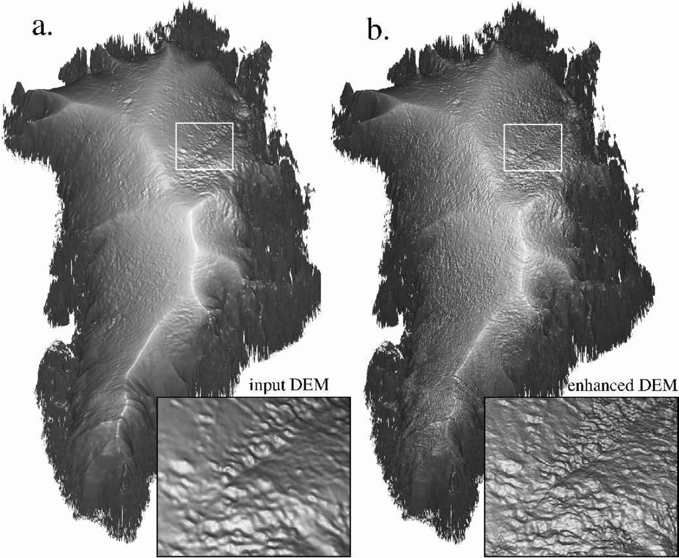
Quantitative interpolation using satellite image data, via photoclinometry, can inexpensively add much of the missing surface elevation detail in this range (Fig. 1). As we demonstrate here, it is an accurate and precise method when its inherent potential for noise at small scales, and drift at large scales, can be constrained by combining it with altimetry-based DEMs.

Fig. 1.

Comparison of the input Reference Bamber, Ekholm and KrabillBamber and others (2001) DEM (a) and the same DEM with more topography added using the described photoclinometric technique (b). Both images are grey-scale representations of absolute slope. Insets to the lower right of each image show the onset region of the northeastern Greenland flow feature in greater detail. The inset areas are 187.5 km by 156 km.

Photoclinometric Method

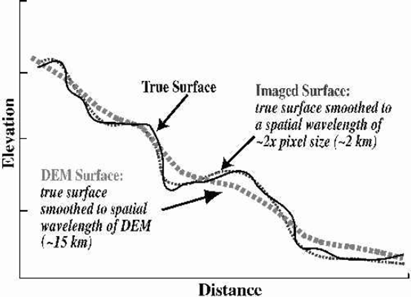
We apply here an improved version of the photoclinometry method described in Reference Scambos and FahnestockScambos and Fahnestock (1998), and extend the regions mapped by the technique to cover the entire Greenland ice sheet. The fundamental method remains the same: we use the digital image brightness to quantitatively determine local surface slope in the direction of solar illumination. We then combine this local detail with a regional elevation field to generate an improved DEM. This approach assumes that the initial DEM is an accurate, but smoothed, representation of the true surface at some scale (Fig. 2).

Fig. 2.

Diagram illustrating DEM and ice-sheet surface morphology

The slope-to-brightness relationship for the images is calibrated by comparison to the same DEM. We determine the relationship of the slopes in the relatively coarse-resolution DEM (derived by some other means) and the brightness of smoothed (low-pass filtered) image pixel values; images smoothed to the resolution of the DEM. We also assume that the slope-to-pixel-brightness relationship will be linear with respect to the cosine of the illumination angle, i.e. that

where DN is the brightness value for the sensor channel in the image, A is a constant related to the sensitivity of the sensor and the albedo of the surface, θ is the surface incidence angle of illumination, and B is a constant related to the threshold value for the sensor and the amount of light scattered into the surface sensor path from other sources (see Reference Bindschadler and VornbergerBindschadler and Vornberger, 1994; Reference Bindschadler, Scambos, Rott, Skvarca and VornbergerBindschadler and others, 2002). We refer to this brightness-to-slope equation as the photofunction. The linear form of the photofunction is based on an assumption of Lambertian reflectance for the snow surface. This approximation would not hold for large ranges of illumination and viewing (see Reference Nolin and LiangNolin and Liang, 2000), but is reasonably accurate for near-nadir images with moderate sun elevations (10–35°).

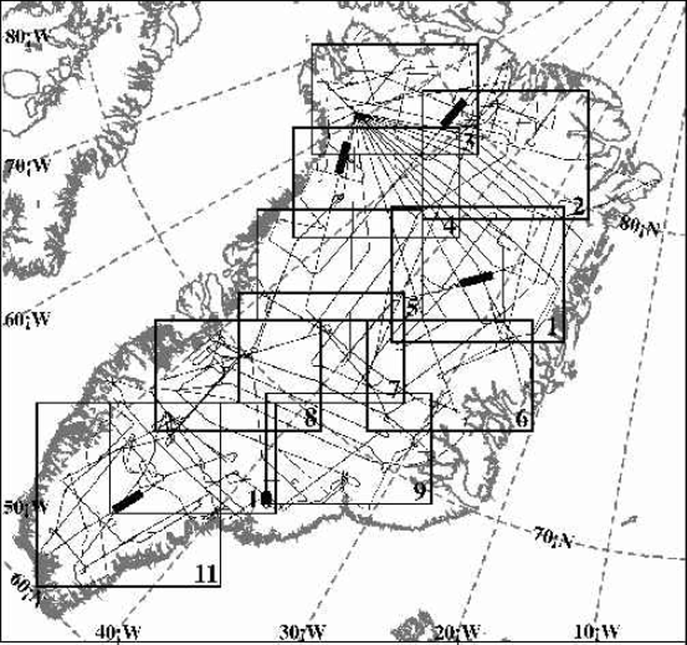
The input DEM was provided by the Danish Cadastral Survey (see Reference Bamber, Hardy and JoughinBamber and others, 2000a, Reference Bamber, Ekholm and Krabill2001). A total of 44 Advanced Very High Resolution Radiometer (AVHRR) images were used in the enhancement, selected on the basis of uniform snow surface, absence of clouds, and wide distribution of illumination azimuths. Springtime images (from 1997) were used because an extensive search of the National Snow and Ice Data Center (NSIDC) archive of polar 1km AVHRR data showed that spring images had fewer clouds and more uniform surface reflectance. The ice sheet was divided into 11 overlapping sub-regions, each approximately 500 km by 400 km (Fig. 3). For each sub-region, between 5 and 11 images were used (some images spanned more than one sub-region). Channel 1of AVHRR was used because of its lower sensitivity to snow grain-size variations (Reference Dozier, Schneider and McGinnisDozier and others, 1981). The imagery was processed to remove the point spread function, a step which attempts to mitigate blurring at the pixel level caused by the sensor system (Reference Reichenbach, Koehler and StrelowReichenbach and others, 1995). We re-projected the images to a common grid, using a Lambert azimuthal equal-area grid with a grid spacing of approximately 625m (see http://nsidc.org/NSIDC/GUIDE/EASE/ease___grid.html); however, we distribute the final elevation grid in a simple latitude–longitude grid.

Fig. 3.

Map of Greenland in the Lambert azimuthal equal-area projection used for image-based enhancement. Numbered boxes indicate sub-regions of photoclinometric enhancement of the DEM. Fine solid lines indicate surface tracks of ATM data used to validate the DEM. The four heavy solid lines indicate 100 km long sections of profiles used in Figure 6.

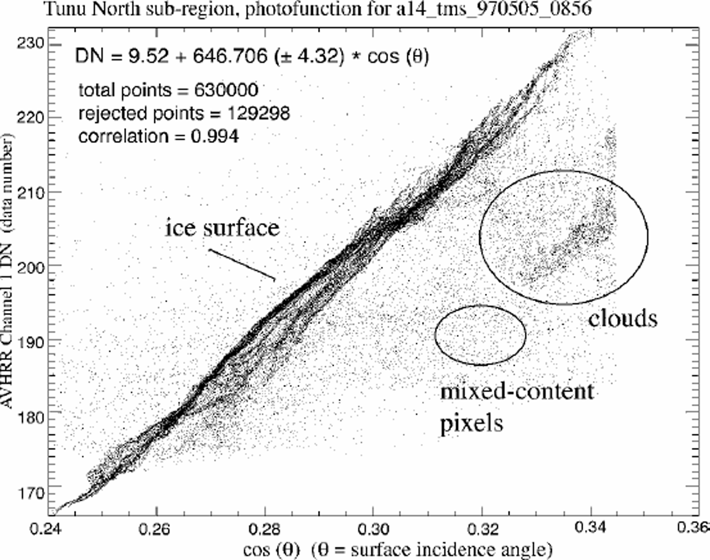
As stated above, the photofunction is determined by comparing the smoothed brightness values for the image with the smoothing scale determined by the resolution of the DEM. We compared a variety of smoothing scales for the images to the input DEM. The image filter scale that best matches the DEM (i.e. the blurring required to have the images look like the shaded relief of the DEM) is equal to *20 km ground equivalent (31 by 31 pixel low-pass filter with 625 m pixels). A typical photofunction plot is shown in Figure 4. Correlations (r) to the linear fit of smoothed brightness vs DEM slope for the 44 images are typically 0.97–0.99. Slope of the photofunction ranges from 444.3 to 1024.2, increasing with solar elevation. Mean photofunction slope is 682.3. Error of the photofunction slope (a measure of the precision of the eventual surface slope determination) was generally <2% of the slope value.

Fig. 4.

Surface incidence angle of illumination vs low-pass filtered AVHRR channel 1 image brightness for a specific image covering the Tunu North sub-region (No. 2 of Fig. 3). Solar elevation for this scene at the center of the sub-region was 26°, and solar azimuth was 174°.

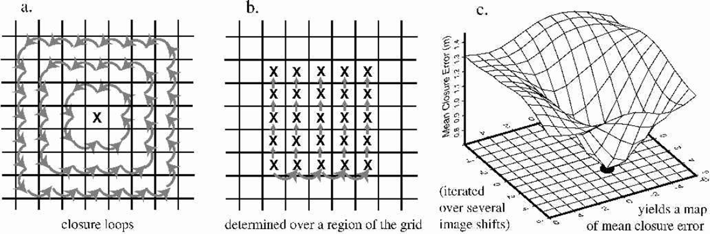
Once the photofunction of each image is determined, pairs of images are co-registered by testing the continuity of the surface they define. For the initial re-projection we use satellite ephemerides and satellite clock time corrections to navigate the pixels onto the projection grid. However, the residual error in this method is still several pixels (1–5 km). Because of the wide variation in solar illumination direction among the images, standard co-registration schemes (e.g. Reference Scambos, Dutkiewicz, Wilson and BindschadlerScambos and others, 1992) cannot be used. Instead we use a scheme based on the assumption that the surface is continuous and that slopes derived from properly registered images should define a smooth surface (differentiable, with no singularities; curl of the divergence equal to zero). To do this, we sequentially try several registrations for a pair of images, and, for each try, determine the two-dimensional slope field defined by the pair given that registration vector. Then the surface elevation closure of small loops of pixels is determined. For perfect grids, perfectly registered, the elevations and slopes should sum to zero in a closed loop. The proper registration vector is determined where the minimum mean closure error of the loops is observed. This was discussed in Reference Scambos and FahnestockScambos and Fahnestock (1998), but the approach was augmented here to provide more robust registration (Fig. 5). Further, since some of the images have similar solar azimuths (and the registration method we use requires wide separation of illumination direction), a matrix of the offsets for various pairings was used to determine an internally consistent set of registration vectors for the image set. A final step determined the absolute registration of the merged DEM by shifting the DEM in x and y until a consistent minimum root-mean-squared (rms) error relative to the Airborne Topographic Mapper (ATM) profiles was observed.

Fig. 5.

Diagram of the improved image-registration algorithm. In practice, steps (a) and (b) are conducted over five areas of the images, and the results averaged to yield a single mean closure error point in (c). Images are shifted +15 grid steps in both directions (rather than +6 as shown here). The heavy dot below the minimum mean closure error represents the selected registration shift; in this example, a shift of [–1, 2] gridcells relative to a master image.

The primary improvement in the photoclinometry procedure used here is the use of multiple images, rather than just two, to provide slope information at a wide range of solar illumination directions. Additionally, we now apply a weighting scheme in which the quality of fit of a specific pixel to the photofunction is used to eliminate noisy, cloudy or mixed-surface-type pixels. This quality of fit approach is also used to weight the valid pixels for each image by comparing the agreement of the image region to the photo-function, which tends to eliminate wind-glazed, thinly cloud-covered, or frost-covered surfaces. The valid pixels are then converted to slopes in the sunward azimuth. The several slopes (from the several images) for each gridcell create an overdetermined system of equations defining the surface normal. Weights for the slopes are used to adjust the least-squares fit of the surface normal to the data for that gridcell. A second iteration, refined by the initial estimate of the surface normal, is run to yield the final best-fit surface normal for the cell. The use of several images, accurately co-registered to less than one sensor pixel precision, also results in some improvement in spatial resolution beyond what is present in a single image (see Reference Scambos, Kvaran and FahnestockScambos and others, 1999).

We explored and discarded an additional correction for grain-size variation across each scene, based on a semiquantitative determination of grain-size using a normalized difference of channels 1 and 2 for AVHRR. In the trial application, we corrected the brightness values of the channel 1 image based on the estimated grain-size from the comparison of channel 1 and 2 reflectance. However, mean grain-size did not vary appreciably across the springtime imagery, and the correlation values of the photofunctions were not improved by the inclusion of a grain-size correction.

Our processing sequence was: re-projection and regridding of the AVHRR and input DEM to the equal-area grid; low-pass filtering of the images to match the real spatial resolution of the input DEM; generation of photofunctions for the images; co-registration of the images to a master image by the surface continuity test; determination of the surface normals for the grid using the photofunction and unfiltered images; integration of the surface slopes (derived from the surface normals) into surface elevations. After processing the 11 overlapping sub-region grids, we merged the grids to compile the DEM, either blending elevations in the overlap areas or masking out noisy or cloud-affected areas with adjacent sub-regions. The photoclinometric modification to the Bamber and others DEM was limited to areas 410 km from rock exposure or severe crevassing; no changes were made to the perimeter regions.

Validation

Accuracy of the new DEM was checked by comparison with airborne laser altimetry profiles acquired in the 1990s by ATM (see Reference Krabill, Thomas, Martin, Swift and FrederickKrabill and others, 1995; Reference Bamber, Ekholm and KrabillBamber and others, 1998). We compared sections of flight elevation profiles to extracted profiles from the image-enhanced DEM and the original, input DEM in over 50 profile areas of Greenland. Four example profiles and the results of their validation tests are shown in Figure 6.

Fig. 6.

Profile comparisons of the input DEM, enhanced DEM and ATM airborne laser elevation tracks. The four profiles are from the four tracks shown in Figure 3 as heavy lines. Note variations in elevation scales for the four profiles.

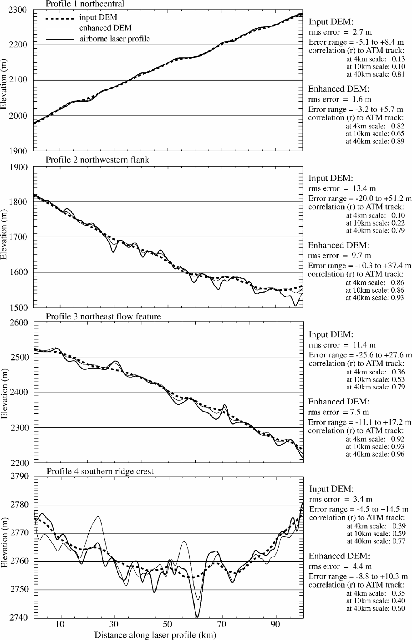
The profiles indicate that undulations of 3–10 km horizontal scale and several tens of meters vertical relief are resolved in the enhanced DEM, and in general are not resolved in the input DEM. The rms error relative to the ATM profiles of the image-enhanced DEM is 0.5–0.8 times that of the input DEM in most areas. There is a similar reduction in the range of maximum deviation from the airborne profiles for the enhanced DEM. However, in areas near the ice-sheet ridge crests (e.g. profile 4 of Fig. 6), where local topography is extremely smooth, the additional high-spatial-frequency noise introduced by the imagery in the enhanced DEM (due to clouds, frost or telemetry noise that was not eliminated by earlier processing) outweighs the improvement in tracking surface undulations. In the vicinity of the major ice-sheet divides (above about 3000 m), rms errors for the Bamber and others DEM were 0.5–4m, and for the image-enhanced DEM were 1.5–5m.

The improvement made by photoclinometry is even more apparent when measured by the correlation of the DEMs to the ATM profiles at high spatial frequencies. This demonstrates that significant frequency content was added by the image enhancement, and the new content correlates with actual undulations (Fig. 6, tables on right side). To do this, we low-pass filtered the original DEM to several spatial scales (4,10 and 40 km) and compared the correlation of residuals between this filtered DEM and the unfiltered ATM, enhanced DEM and input DEM profiles. In most regions the enhanced DEM has a much higher positive correlation with the residual ATM undulations than the original DEM, as the filtering scale is reduced below 15 km (Fig. 6, tables for profiles 1–3). The exceptions are, again, in the vicinity of the ridge crests of the ice sheet, where very little high-frequency topography exists. The enhanced DEM recovered nearly all topographic features of 43 km horizontal scale. The limiting resolution of the input DEM is approximately 15 km. For both DEMs, as the spatial scale approaches the limiting resolution, the amplitude of the represented topography is reduced.

Perfect agreement with the ATM profiles (at any filtering scale) should not be expected for either the input DEM or the improved image-enhanced DEM. At least part of the rms error, and the reduced relief of DEMundulations, must be attributed to the different sampling of the surface by the laser altimeter (a helical scan smoothed to a swath of mean elevations 140m wide) vs the AVHRR sensor (1.1km pixel spacing, sampling a region approximately 1.5 km across) and the satellite radar altimeter (having a beamwidth of approximately 2 km and ground-track separations of up to several kilometers). The coarser sampling of the surface for the imaging sensor and satellite radar altimeter, and the two-dimensional interpolation of the data to create the DEMs, results in an inherent low-pass filtering of the surface relative to that measured by the narrow-swath, high-spatialfidelity laser profiler.

Features Revealed By The Enhanced Dem

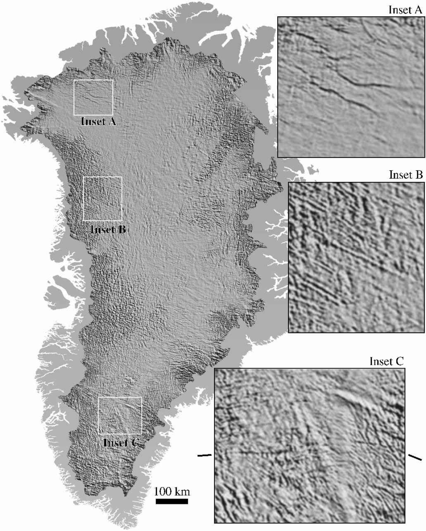
The enhanced DEM resolves several features almost certainly related to bedrock morphology, adding important detail to these features relative to the input DEM (Fig. 7). In inset A of Figure 7, a pair of troughs a few kilometers wide underlying the onset regions for Humbolt Gletscher may represent sub-areal paleo-drainage features. The enhanced DEM has about 14 m relief across the features, and they can be traced for over 100 km in the direction of the coast. Ice thickness in this area is about 1500m (Reference Escher and PulvertaftEscher and Pulvertaft, 1995). In several areas along the eastern and western flanks, distinct preferred orientations of small undulations in the ice sheet suggest that the bedrock beneath these areas has strong layering or foliation. Inset B shows such an area inland from the Lauge Koch Cyst region of West Greenland. Ice thickness in this area ranges from about 1750 to 2250 m. Inset C shows a curvilinear trough crossing most of the southern portion of the ice sheet, at least 200 km long and up to 22 mdeep. This feature is mapped as a possible intraplate transform fault in Reference Escher and PulvertaftEscher and Pulvertaft (1995).

Fig. 7.

Shaded-surface representation of the enhanced surface topography of the Greenland ice sheet, high-pass filtered to 15 km. Insets show regions of interest at full resolution. The ticks next to inset C indicate the trend of the feature thought to be due to the transform fault. The scale bar pertains to the main image; insets are magnified by a factor of four.

Bedrock Topography And The Enhanced Dem

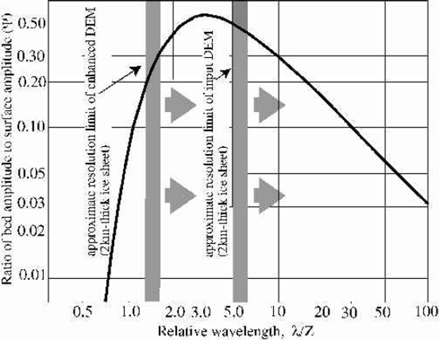
The possibility of deriving quantitative bedrock topography from inverting a surface elevation dataset using a model of ice flow over the bedrock surface has been discussed several times in the literature (e.g. Reference BuddBudd, 1970; Reference Whillans and JohnsenWhillans and Johnsen, 1983; Reference Fastook, Brecher and HughesFastook and others, 1995). Budds model of the ice flow over harmonic bedrock perturbations assumed a low mean surface slope and required that most of the deformation, sliding or shear, takes place near the bed surface; conditions which apply reasonably well to most of the interior Greenland ice sheet. Figure 8 is a plot of the damping function derived by Reference BuddBudd (1970) as a function of relative wavelength, i.e. the horizontal scale of the bed topographic features in units of ice thickness. The scale at which bed features are best represented in the surface topography, or minimum damping scale, is 3.3 ice thicknesses. Bedrock features should be represented by surface undulations with roughly half their true amplitude at this scale, and the damping factor is 40.2 over the range 1.5–15 ice thicknesses. For the flanking areas of Greenland, such as the undulating areas of Figure 7, ice thickness ranges from about 1000 to 2500 m; thus the horizontal scale at which most information about bed structure might be obtained lies between 1.5 and a few tens of kilometers. Figure 8 illustrates that an important fraction of the bed-related surface topography is contained in the enhanced DEM, and that approximately quantitative measurement of bed elevation at a resolution as fine as 3–5km should now be possible.

Fig. 8.

Filter function relating bedrock undulation amplitude to surface undulation amplitude for ice sheets. The minimum damping occurs at 3.3 times the ice thickness. Modified fromfigure 3b of Reference BuddBudd (1970) (symbols for variables are from his equations).

Summary

Imagery can be used to quantitatively add detail to DEMs over ice sheets, and that detail can reveal important features related to bed topography. We expect that the enhanced DEM will also be important to the interpretation of recently identified accumulation variations associated with the pattern of wind redistribution of snow over the undulation field. Although some noise is added to the input elevation field, the increased spatial resolution results in a reduced rms error and an increased correlation to the fine-scale undulation field, over most of the ice sheet. The enhanced DEM is an accurate representation of the mean elevation of the ice sheet at a scale of 3 km, with an error of ±4m. The input DEM is an accurate representation of the mean elevation at a scale of 15 km, with an error of +2 m.

The 625m DEM of the Greenland ice sheet we have developed is available upon request, subject to the restrictions on distribution of the input DEM (see the NSIDC website on DEMs for Greenland for information).