








1 Introduction
Let
 $(a_n)_{n=1}^\infty $
be a strictly increasing sequence of positive integers. This paper is concerned with the distribution of
 $(\alpha a_n \, \text {mod } 1)_{n=1}^\infty $
in short intervals, for a generic dilate
 $\alpha \in [0,1]$
, with particular focus on the case when
 $a_n = n^2$
.
We begin with the familiar notion of the discrepancy
 $D_N = D_N((\alpha a_n \, \text {mod } 1)_{n=1}^\infty )$
, defined to be
 $$ \begin{align} D_N = \mathop{\mathrm{sup}}\limits_{0<a<b<1} \left\vert \frac{\vert \{n\leq N: \alpha a_n \, \text{mod }1 \in (a,b)\} \vert}{N} - (b-a) \right\vert. \end{align} $$
It is an old result of Weyl, contained in his 1916 paper [Reference Weyl29], that
 $ D_N((\alpha n^2 \, \text {mod } 1)_{n=1}^\infty ) = o_{\alpha }(1)$
as
 $N\rightarrow \infty $
for any irrational
 $\alpha $
. The sequence
 $(\alpha n^2 \, \text {mod } 1)_{n=1}^\infty $
is then said to be equidistributed modulo
 $1$
. One way of viewing Weyl’s result is as demonstrating a pseudorandomness property for the sequence
 $(\alpha n^2 \, \text {mod } 1)_{n=1}^\infty $
. Indeed, in the random model in which
 $( \alpha n^2 \, \text {mod } 1)_{n=1}^N$
is replaced by N independent random variables
 $X_1,\dots ,X_N$
, which are uniformly distributed on
 $[0,1)$
, one hasFootnote
1
 $$ \begin{align*}\limsup_{N\rightarrow \infty} \frac{ \sqrt{2N} D_N((X_n)_{n=1}^\infty)}{\sqrt{\log \log N}} = 1 \end{align*} $$
almost surely. In particular
 $\mathbb {E}D_N((X_n)_{n=1}^\infty ) = o(1)$
as
 $N\rightarrow \infty $
.
One might wonder, considering the strong quantitative decay enjoyed in the random model, whether Weyl’s result admits such a quantitative refinement. Unfortunately, as is well known, if
 $\alpha $
is well approximated by rational numbers with small denominators, then the discrepancy
 $D_N((\alpha n^2 \, \text {mod } 1)_{n=1}^\infty )$
can tend to zero extremely slowly. However, for a generic
 $\alpha $
, the situation is much improved, and in fact, for any strictly increasing sequence of positive integers
 $(a_n)_{n=1}^\infty $
, one has the classical result of Erdős and Koksma [Reference Erdős and Koksma9], which implies that
 $$ \begin{align*}D_N((\alpha a_n \, \text{mod } 1)_{n=1}^\infty) = O_{\varepsilon}(N^{-\frac{1}{2} + \varepsilon})\end{align*} $$
for Lebesgue almost all
 $\alpha \in [0,1]$
. This trivially implies that, for almost all
 $\alpha \in [0,1]$
, if
 $I \subset \mathbb {R}/\mathbb {Z}$
is a fixed interval of length
 $\vert I\vert \geqslant N^{-\frac {1}{2} + \varepsilon }$
, then
 $$ \begin{align} \vert \{ n \leqslant N: \alpha n^2 \, \text{mod } 1 \in I\}\vert = (1 +o_{\varepsilon}(1)) N \vert I\vert. \end{align} $$
So, at least for a generic
 $\alpha $
, pseudorandomness is enjoyed down to the scale
 $N^{-1/2 + \varepsilon }$
. A result of Aistleitner and Larcher [Reference Aistleitner and Larcher1, Corollary 1] implies that the exponent
 $\tfrac {1}{2}$
is optimal for the metric discrepancy problem: for generic
 $\alpha $
and for each
 $\varepsilon>0$
, there are infinitely many N such that
 $ D_N((\alpha a_n \, \text {mod } 1)_{n=1}^\infty )> N^{-1/2 -\varepsilon }$
, provided
 $a_n = P(n)$
for some polynomial P, of degree at least two, with integer coefficients.
By allowing the interval I to vary, one can develop a related notion of pseudorandomness at scales that are smaller than
 $N^{-1/2}$
, one which concerns the “clustering” of the points
 $\alpha n^2 \, \text {mod } 1$
. To introduce this notion, which will be the main focus of the paper, we let Y be a random variable that is uniformly distributed on
 $[0,1)$
, and for a natural number N and a parameter L in the range
 $0 < L \leqslant N$
, we let
 $W_{\alpha , L,N}$
be the random variable
 $$ \begin{align} W_{\alpha, L,N}:=\vert \{n \leqslant N :\alpha n^2\in [Y,Y+L/N] \, \text{mod } 1\}\vert. \end{align} $$
It is easy to see that
 $\mathbb {E} W_{\alpha ,L,N} = L$
. But how should one expect
 $W_{\alpha ,L,N}$
to be distributed in the limit
 $N \rightarrow \infty $
(for a generic dilate
 $\alpha $
)? Consider the same random model as before, in which
 $( \alpha n^2 \, \text {mod } 1)_{n=1}^N$
is replaced by N independent random variables
 $X_1,\dots ,X_N$
, which are uniformly distributed on
 $[0,1)$
. Then, if L is constant as
 $N \rightarrow \infty $
, letting
 $$ \begin{align} Z_{L,N} := \vert\{n \leqslant N : X_n \in [Y,Y+L/N] \, \text{mod } 1 \}\vert, \end{align} $$
one may calculate that
 $$ \begin{align*} Z_{L,N} \xrightarrow{dist} \operatorname{Po}(L) \end{align*} $$
as
 $N \rightarrow \infty $
, where
 $\operatorname {Po}(L)$
is a Poisson-distributed random variable with parameter L.
Having described this random model, we can now state the following remarkable conjecture.
Conjecture 1.1 (Rudnick and SarnakFootnote 2 [Reference Rudnick and Sarnak23].)
For almost all
 $\alpha \in [0,1]$
, for all fixed
 $L>0$
,
 $$ \begin{align*} W_{\alpha,L,N} \xrightarrow{dist} \operatorname{Po}(L),\end{align*} $$
as
 $N \rightarrow \infty $
.
If true, this conjecture would represent a strong local notion of pseudorandomness for the sequence
 $(\alpha n^2 \, \text {mod } 1)_{n=1}^\infty $
, at least for a generic
 $\alpha $
. In fact, a further conjecture [Reference Rudnick, Sarnak and Zaharescu24, p. 38] posits more information about the full-measure set of suitable dilates
 $\alpha $
. To state this conjecture, we recall that
 $\alpha $
is of type
 $\omega $
if there are only finitely many pairs
 $(a,q)$
with
 $\vert \alpha - a/q\vert < q^{-\omega }$
.
Conjecture 1.2 (Rudnick, Sarnak, and Zaharescu.)
If
 $\alpha $
is of type
 $2 + \varepsilon $
for all
 $\varepsilon>0$
, and the convergents
 $a/q$
to
 $\alpha $
satisfy
 $$ \begin{align*}\lim\limits_{ q \rightarrow \infty} \log \widetilde{q} / \log q = 1,\end{align*} $$
where
 $\widetilde {q}$
is the square-free part of q, then, for all fixed
 $L>0$
, as
 $N \rightarrow \infty $
, one has
 $$ \begin{align*} W_{\alpha,L,N} \xrightarrow{dist} \operatorname{Po}(L).\end{align*} $$
Remark: We remind the reader that, by Dirichlet’s approximation theorem, the type of a real number is never less than
 $2$
. Furthermore, by Khintchine’s theorem, a generic number is of type
 $2+\varepsilon $
for all
 $\varepsilon>0$
. One can also readily find explicit examples, like
 $\alpha = \sqrt {2}$
, by using continued fractions.
Conjectures 1.1 and 1.2 appear to lie very deep. One hypothetical approach for showing the desired convergence in distribution would be to use the method of moments. More precisely, if one could show, for a generic
 $\alpha $
, for a random variable
 $X_L \sim \operatorname {Po}(L)$
, and for all
 $k \in \mathbb {N}$
, that
 $\operatorname *{\mathrm {\mathbb {E}}} W_{\alpha , L,N}^k \rightarrow \operatorname *{\mathrm {\mathbb {E}}} X_L^k$
as
 $N \rightarrow \infty $
, then Conjecture 1.1 would follow. Rudnick and Zaharescu [Reference Rudnick and Zaharescu25] used this approach to show that if
 $(a_n)_{n=1}^\infty $
is a lacunary sequence of natural numbers, then, for almost all
 $\alpha $
, the sequence
 $(\alpha a_n \, \text {mod } 1)_{n=1}^\infty $
has spacing statistics that agree with the Poisson model. For the squares, the first nontrivial case is
 $k = 2$
, and this was settled by Rudnick and SarnakFootnote
3
some 22 years ago.
Theorem 1.3 (Rudnick and Sarnak [Reference Rudnick and Sarnak23])
For almost all
 $\alpha \in [0,1]$
, for all fixed
 $L>0$
,
 $$ \begin{align*} \mathbb{E} W_{\alpha,L,N}^2 = L + L^2 + o_{\alpha,L}(1),\end{align*} $$
as
 $N \rightarrow \infty $
.
This gives an estimate on the so-called number variance
 $\operatorname {Var}(W_{\alpha ,L,N})$
, namely
 $$ \begin{align*} \operatorname{Var}(W_{\alpha,L,N}) = L +o_{\alpha, L}(1),\end{align*} $$
as
 $N \rightarrow \infty $
.
Very little is known regarding the higher moments, although certain results can be extracted from the literature. For larger L, the issue is settled by the aforementioned discrepancy bounds. Indeed, expression (1.2) implies that, for almost all
 $\alpha \in [0,1]$
, for all integers
 $k \geqslant 1$
, for all
 $N \in \mathbb {N}$
, and for all
 $L \in \mathbb {R}$
in the range
 $ N^{1/2 + \varepsilon } \leqslant L \leqslant N$
,
 $$ \begin{align} \mathbb{E} W_{\alpha,L,N}^k = L^k(1 + o_{\alpha,\varepsilon,k}(1)), \end{align} $$
as
 $N \rightarrow \infty $
(where the error term is independent of the choice of parameters L). We will give the simple proof of (1.5) in Appendix B, alongside other consequences of the discrepancy bounds. In passing, we will answer a question of Steinerberger from [Reference Steinerberger27].
One might wonder whether the methods that Rudnick and Sarnak introduced to tackle the second moment in Theorem 1.3 could be applied to higher moments. Unfortunately, in the case when L is constant, Rudnick and Sarnak already noted in [Reference Rudnick and Sarnak23, Section 4] that their method faces a major obstruction when applied to higher moments. We will describe this obstruction in Appendix C, where (for the third moment) we observe that the obstruction persists for L as large as
 $N^{1/3}$
.
We now present the main result of this paper.
Theorem 1.4 (Main Theorem)
Let
 $\varepsilon>0$
. Then, for almost all
 $\alpha \in [0,1]$
, for all
 $N \in \mathbb {N}$
, and for all
 $L \in \mathbb {R}$
in the range
 $N^{1/4 + \varepsilon } < L \leqslant N$
, we have
 $$ \begin{align*} \mathbb{E} W_{\alpha,L,N}^3 = L^3(1 + o_{\alpha, \varepsilon}(1)),\end{align*} $$
as
 $N\rightarrow \infty $
, where the
 $o_{\alpha ,\varepsilon }(1)$
term is independent of the choice of the parameters L.
Note, in particular, that
 $\tfrac {1}{4} < \tfrac {1}{3}$
, so we successfully give an asymptotic expression for the third moment in part of the range in which the Rudnick–Sarnak obstruction holds (see Appendix C).
To prove Theorem 1.4, we will first perform a standard reduction to a statement concerning correlation functions. These functions are closely related to the moments
 $\mathbb {E} W_{\alpha ,L,N}^k$
, but they can be more convenient to analyze.
Definition 1.1 (Correlation functions)
Let
 $\alpha \in [0,1]$
, let
 $k \geqslant 2$
be a natural number, and let
 $g:\mathbb {R}^{k-1} \rightarrow [0,1]$
be a compactly supported function. Then, the kth correlation function
 $R_k(\alpha ,L,N, g)$
is defined to be
 $$ \begin{align*}\frac{1}{N}\sum\limits_{\substack{1 \leqslant x_1, \dots, x_k \leqslant N \\ \text{distinct}}} g\left(\frac{N}{L} \{ \alpha (x_1^2 - x_2^2)\}_{\operatorname{sgn}}, \frac{N}{L}\{ \alpha (x_2^2 - x_3^2)\}_{\operatorname{sgn}}, \dots, \frac{N}{L}\{ \alpha (x_{k-1}^2 - x_k^2)\}_{\operatorname{sgn}}\right),\end{align*} $$
where
 $$ \begin{align*} \{ \cdot \}_{\operatorname{sgn}}:\mathbb{R} \longrightarrow (-1/2,1/2]\end{align*} $$
denotes the signed distance to the nearest integer, and N and L are real parameters.
In practice, one only needs to understand the correlation functions when the test function g is sufficiently nice, for example, smooth or the indicator function of a box.
When proving Theorem 1.3, Rudnick and Sarnak manipulated the pair correlation function
 $R_2(\alpha ,L,N,g)$
. We manipulate the triple correlation function
 $R_3(\alpha ,L,N,g)$
, proving the following result, which, for readers more familiar with correlation functions than with the moments of
 $W_{\alpha ,L,N}$
, might seem to be more natural.
Theorem 1.5 (Triple correlations)
Let
 $\varepsilon>0$
. Then, for almost all
 $\alpha \in [0,1]$
, for all compactly supported continuous functions
 $g: \mathbb {R}^2 \longrightarrow [0,1]$
, for all
 $N \in \mathbb {N}$
, and for all
 $L \in \mathbb {R}$
in the range
 $N^{1/4 + \varepsilon } < L < N^{1- \varepsilon }$
, we have
 $$ \begin{align*} R_3(\alpha,L,N,g) = (1 + o_{\alpha,\varepsilon, g}(1))L^2 \left(\int g(\mathbf{w}) \, d\mathbf{w}\right),\end{align*} $$
as
 $N \rightarrow \infty $
, where the
 $o_{\alpha ,\varepsilon ,g}(1)$
term is independent of the choice of the parameters L.
Before continuing to survey other relevant papers, we should stop to explain why the spacing statistics of the sequence
 $\alpha n^2 \, \text {mod } 1$
are of a particular interest (aside from as a part of the larger endeavor of finding pseudorandomness in arithmetic sequences). This is due to a connection between number theory and theoretical physics known as arithmetic quantum chaos. In brief, the spacing statistics between elements of the sequence of
 $\alpha n^2 \, \text {mod } 1$
correspond to the spacing statistics between the eigenvalues of a certain quantum system. (This system is a two-dimensional boxed oscillator, with a harmonic potential in one direction and hard walls in the other, as described in the introduction to [Reference Rudnick and Sarnak23].) A famous and far-reaching observation of Berry and Tabor [Reference Berry and Tabor4] then suggests that such spacing statistics in the semiclassical limit (i.e., the distribution of
 $W_{\alpha ,L,N}$
for constant L as
 $N \rightarrow \infty $
) should be determined by the dynamics of the corresponding classical system. Regular (integrable) classical dynamics should correspond to spacing statistics in asymptotic agreement with the Poisson model.
Unfortunately, if
 $\alpha $
is rational (or is very well approximated by rationals with square denominators), it is easy to prove that high moments of
 $W_{\alpha ,L,N}$
do not agree with the Poisson model (see [Reference Rudnick, Sarnak and Zaharescu24, Theorem 2])! However, excluding such zero-measure counter-examples,Footnote
4
one might still hope for a metric result.
There are precious few examples of fixed sequences for which full information is known about the spacing statistics. For the sequence
 $(\sqrt {n} \, \text {mod } 1)_{n=1}^{\infty }$
, Elkies and McMullen [Reference Elkies and McMullen8] have established, using dynamical methods, the gap distribution of
 $(\sqrt {n} \, \text {mod } 1)_{n=1}^{\infty }$
(which is not from a Poisson model); El-Baz, Marklof, and Vinogradov [Reference El-Baz, Marklof and Vinogradov7] have demonstrated that the second moment of this gap distribution is nonetheless in accordance with the Poisson model. Furthermore, there are the results in [Reference Eskin, Margulis and Mozes10] and [Reference Marklof18] on the second moment of the gap distribution between values of quadratic forms. However, most of the results in the literature are metric in at least one parameter (e.g., [Reference Aistleitner, Larcher and Lewko2, Reference Rudnick and Sarnak23, Reference Rudnick and Zaharescu25, Reference Sarnak26]), and such results still have substantial content.
To delve further into the relationship to theoretical physics and to other, spacing statistics would be to digress too far from our main theme; we direct the interested reader to the articles of Marklof [Reference Marklof, Casacuberta, Miró-Roig, Verdera and Xambó-Descamps17] and Rudnick [Reference Rudnick20] for more on these issues.
Returning to the study of the moments of
 $W_{\alpha ,L,N}$
, and the discussion of relevant work, we continue with the paper [Reference Rudnick, Sarnak and Zaharescu24]. Here, Rudnick, Sarnak, and Zaharescu develop tools to relate the Diophantine approximation properties of
 $\alpha $
to the size of the moments
 $\mathbb {E} W_{\alpha ,L,N}^k$
. The main result of that paper can be phrased as follows.
Theorem 1.6 (Rudnick, Sarnak, and Zaharescu)
Let
 $\alpha \in [0,1]$
, and suppose that there are infinitely many rationals
 $b_j/q_j$
, with
 $q_j$
prime, satisfying
 $$ \begin{align} \left\vert \alpha - \frac{b_j}{q_j}\right\vert < \frac{1}{q_j^3}. \end{align} $$
Then, there is a subsequence
 $N_j \rightarrow \infty $
, with
 $ \log N_j/ \log q_j \rightarrow 1$
for which, for all
 $L>0$
,
 $$ \begin{align*} W_{\alpha,L,N_j} \xrightarrow{dist} \operatorname{Po}(L),\end{align*} $$
as
 $j \rightarrow \infty $
.
The authors of [Reference Rudnick, Sarnak and Zaharescu24] sacrificed the genericness of
 $\alpha $
(working instead with those
 $\alpha $
which are unusually well-approximable) in favor of control over the moments
 $\mathbb {E} W_{\alpha ,L,N_j}^k$
for constant L and for all k. One may switch objectives in their analysis, sacrificing the range of L in order to work with almost all
 $\alpha $
. Applying this switch in the context of the third moment calculation, their method shows the following result.
Theorem 1.7 (Method of R–S–Z)
Let
 $\varepsilon>0$
. Then, for almost all
 $\alpha \in [0,1]$
, for all
 $N \in \mathbb {N}$
, and for all
 $L \in \mathbb {R}$
in the range
 $N^{3/5 + \varepsilon } < L \leqslant N$
, we have
 $$ \begin{align*} \mathbb{E} W_{\alpha,L,N}^3 = L^3(1 + o_{\alpha,\varepsilon}(1)),\end{align*} $$
as
 $N \rightarrow \infty $
, where the
 $o_{\alpha ,\varepsilon }(1)$
term is independent of the choice of parameters L. Moreover, one can give an explicit description of a suitable full-measure set of suitable
 $\alpha $
(in terms of properties of rational approximations to
 $\alpha $
).
Although the range of L in Theorem 1.7 is much smaller than the range in our result, the method of R–S–Z yields a more explicit description of the full-measure set of suitable
 $\alpha $
. We will indicate how to extract Theorem 1.7 from [Reference Rudnick, Sarnak and Zaharescu24] in Section 3 below.
Our approach to proving Theorem 1.5 is inspired by this work of R–S–Z, but also by the work of Heath-Brown in [Reference Heath-Brown12], who introduced a related technique for studying the pair correlation function
 $R_2(\alpha , L,N,g)$
. The full description of the method will come in Section 3, but we sketch the idea here, so as to explain in a rough way how we extract an improvement over [Reference Rudnick, Sarnak and Zaharescu24]. After having replaced
 $\alpha $
by a rational approximation
 $a/q$
, one transforms the triple correlation function into an expression that counts the number of solutions to certain polynomial equations modulo q. The equations which occur are of the form
 $$ \begin{align} \{ x,y,z \leqslant N: x^2 - y^2 \equiv c_1 \,(\text{mod } q), y^2 - z^2 \equiv c_2 \, (\text{mod } q)\}, \end{align} $$
for certain ranges of N and q and for certain sets of coefficients
 $c_1$
and
 $c_2$
. In [Reference Rudnick, Sarnak and Zaharescu24], the number of solutions was estimated by using the “completion of sums” technique to remove the N cutoff, followed by an implementation of the Hasse–Weil bound. In our work, we manage to take advantage of the extra averaging over
 $c_1$
and
 $c_2$
, which is present in the problem, together with some intricate (although elementary) exponential sum arguments, which ends up leading to a stronger bound for certain ranges of N and q. Heath-Brown did something similar for the pair correlation function [Reference Heath-Brown12], but the analysis of the relevant exponential sums for the triple correlations is substantially more delicate.
Another relevant work is the paper of Rudnick and Kurlberg [Reference Rudnick and Kurlberg22], in which those authors established that the spacing of quadratic residues mod q as the number of prime factors of q grows is in agreement with the Poisson model. Lemma 3.3 below could be viewed as a special case of the arguments of that paper. However, as will become evident, the work here necessarily concerns a rather sparse subset of the set of quadratic residues mod q, as
 $N \approx q^{\theta }$
with
 $\theta < 1$
, and so the work of [Reference Rudnick and Kurlberg22] is not directly applicable. Pair correlations of rational functions mod q were also studied by Boca and Zaharescu [Reference Boca and Zaharescu5], but again, we will not be able to use that paper directly.
Very recently, and after the first version of the present manuscript was submitted, Lutsko released a preprint [Reference Lutsko16] which generalized Theorem 1.5 to all long-range correlation functions
 $R_k(\alpha ,L,N,g)$
, provided
 $L \geqslant N^{\frac {k-2}{2k-2} + \varepsilon }$
. When
 $k=3$
, the threshold
 $\frac {k-2}{2k-2}$
recovers our threshold of
 $N^{1/4}$
for triple correlations. Note also that
 $\frac {k-2}{2k-2} \rightarrow \tfrac {1}{2}$
from below as
 $k \rightarrow \infty $
, that is, Lutsko’s threshold approaches the trivial discrepancy bound for large k. The methods of [Reference Lutsko16] seem to be completely different to our own, and are instead based on an analysis of the sums
 $\sum _{n \leqslant N} e(\alpha m n^2)$
using the van der Corput B process (and subsequent stationary phase estimates). It remains to be seen whether any improvement to the threshold
 $c_3 = \tfrac {1}{4}$
could be derived by combining these two different approaches.
The structure of the paper is as follows. In Section 2, we will give the standard argument (passing from moments to correlation functions), which reduces Theorem 1.4 to Theorem 1.5. The proof of Theorem 1.5 is then given in Section 3, in which it is resolved subject to three auxiliary results (one concerning Diophantine approximation, and the other two concerning the number of solutions to certain Diophantine equations similar to (1.7)). The final three sections of the paper settle these results—one per section—thus concluding the main proof.
Appendices A–C contain some arguments that are minor modifications of the literature (but which are nonetheless pertinent to the main paper). These are, respectively, a version of Theorem 1.3 in which L grows with N, the proof of the asymptotic (1.5), and the discussion of the obstruction to the study of triple correlations that was identified by Rudnick and Sarnak.
1.1 Notation
Most of our notation is standard, but perhaps we should highlight a few conventions. For a natural number q, we let
 $e_q(x)$
be a shorthand for
 $e^{2 \pi i x/q}$
, and given a parameter
 $M\geqslant 1$
, we let
 $[M]$
denote the set
 $\{m \in \mathbb {N}: 1 \leqslant m \leqslant M\}$
. In particular,
 $1_{[M]}$
denotes the indicator function of all the natural numbers at most M. If a range of summation is given as
 $\sum _{m \leqslant M}$
, then it is assumed that m is a natural number and that
 $m \geqslant 1$
. Finally, for
 $x \in \mathbb {R}$
, we will use
 $\Vert x\Vert $
to denote the distance from x to the nearest integer, and
 $\{x\}_{\operatorname {sgn}}$
to denote the signed distance to the nearest integer from x.
2 Reduction to correlation functions
In this short section, we will reduce Theorem 1.4 to Theorem 1.5. First, because estimate (1.5) holds for large L, we may assume, without loss of generality, that
 $L < N^{1- \varepsilon }$
. Then, we use linearity of expectation to deduce that
 $$ \begin{align} \mathbb{E}W_{\alpha,L,N}^3 &= \sum\limits_{x,y,z \leqslant N} \mathbb{P}(\alpha x^2, \alpha y^2, \alpha z^2 \in [Y,Y + L/N] \, \text{mod } 1) \nonumber\\ & = \sum\limits_{x \leqslant N} \mathbb{P}(\alpha x^2 \in [Y,Y+L/N] \, \text{mod } 1) \nonumber\\ & \quad + 3 \sum\limits_{ \substack{ x,y \leqslant N \\ x \neq y}} \mathbb{P}(\alpha x^2, \alpha y^2 \in [Y,Y+L/N] \, \text{mod } 1) \nonumber \\ & \quad + \sum\limits_{ \substack{ x,y,z, \leqslant N \\ \text{distinct}}} \mathbb{P}(\alpha x^2, \alpha y^2 , \alpha z^2 \in [Y,Y+L/N] \, \text{mod } 1), \end{align} $$
where Y is a random variable that is uniformly distributed modulo
 $1$
. The first of the three terms in (2.1) is equal to L, and so may be absorbed into the error term of Theorem 1.4. The second term is
 $$ \begin{align} =& 3 \sum\limits_{ \substack{ x,y \leqslant N \\ x \neq y\\ \Vert \alpha(x^2-y^2)\Vert\leqslant L/N}} \left( \frac{L}{N} - \Vert \alpha (x^2 - y^2)\Vert\right) \nonumber\\ =& 3L \left(\frac{1}{N} \sum\limits_{ \substack{x,y, \leqslant N \\ x \neq y}} \max \left(0, 1 - \frac{N}{L}\Vert \alpha(x^2 - y^2)\Vert\right)\right)\nonumber \\ =& 3L R_2(\alpha,L,N,f), \end{align} $$
where
 $f:\mathbb {R} \longrightarrow [0,1]$
is the function
 $f(x) = \max (0,1 - \vert x\vert )$
and
 $R_2(\alpha ,L,N,f)$
is the pair correlation function as defined in Definition 1.1. In Appendix A, we will show, by a trivial adaptation of the known techniques, that, for almost all
 $\alpha \in [0,1]$
, one has
 $$ \begin{align} R_2(\alpha,L,N,f) = (1 + o_{\alpha,f}(1))L \left(\int f(x) \, dx\right) = (1 + o_{\alpha, f}(1))L. \end{align} $$
Therefore, expression (2.2) is equal to
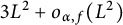 $3L^2 + o_{\alpha ,f}(L^2)$
, which may also be absorbed into the error term of Theorem 1.4.
What remains is the third term of (2.1). This is equal to
 $$ \begin{align} \frac{L}{N} \sum\limits_{ \substack{ x,y,z \leqslant N \\ \text{distinct}}}\max(0,( 1 - \frac{N}{L}\max(\Vert \alpha(x^2 - y^2)\Vert, \Vert \alpha(y^2 - z^2)\Vert, \Vert \alpha(z^2 - x^2)\Vert)). \end{align} $$
Because
 $(x^2 - y^2) + (y^2 - z^2) = x^2 - z^2$
, we see that (2.4) is equal to an expression of the form
 $R_3(\alpha ,L,N,g)$
for some continuous compactly supported function
 $g:\mathbb {R}^2 \longrightarrow [0,1]$
. Indeed,
 $$ \begin{align*} g(w_1,w_2) = \begin{cases} \max(0, 1 - w_1 - w_2) & w_1,w_2 \geqslant 0, \\ \max(0, 1 - \max(w_1, -w_2)) & w_1 \geqslant 0, \, w_2 \leqslant 0, \\ \max(0, 1 - \max(-w_1,w_2)) & w_1 \leqslant 0, \, w_2 \geqslant 0, \\ \max(0, 1 + w_1 + w_2) & w_1, w_2 \leqslant 0. \end{cases} \end{align*} $$
An elementary calculation then demonstrates that
 $$ \begin{align*} \int\limits_{-\infty}^{\infty} \int\limits_{-\infty}^{\infty} g(w_1,w_2) \, dw_1\, dw_2 = 1.\end{align*} $$
Therefore, by Theorem 1.5, if
 $L> N^{\frac {1}{4} + \varepsilon }$
, then, for almost all
 $\alpha \in [0,1]$
, expression (2.4) is equal to
 $L^3(1 + o_{\alpha ,\varepsilon }(1))$
as
 $N \rightarrow \infty $
. So Theorem 1.4 is proved.▪
We make the usual remark that, by approximating the continuous function g above and below by step functions, to prove Theorem 1.5, it will be enough to prove the following result.
Theorem 2.1 Let
 $\varepsilon>0$
. Then, for almost all
 $\alpha \in [0,1]$
, for all
 $s_1,t_1,s_2,t_2 \in \mathbb {R}$
for which
 $s_1 < t_1$
and
 $s_2 < t_2$
, and for all L in the range
 $N^{1/4 + \varepsilon }<L<N^{1- \varepsilon }$
, we have
 $$ \begin{align*} R_3(\alpha,L,N,g_{\mathbf{s},\mathbf{t}}) = (1 + o_{\alpha,\varepsilon, \mathbf{s},\mathbf{t}}(1))L^2 (t_1 - s_1)(t_2 - s_2),\end{align*} $$
as
 $N\rightarrow \infty $
, where
 $\mathbf {s} = (s_1,s_2)$
,
 $\mathbf {t} = (t_1,t_2)$
, and
 $g_{\mathbf {s},\mathbf {t}}$
is the indicator function of the box
 $[s_1,t_1] \times [s_2,t_2]$
.
It will turn out to be crucial in our subsequent methods that the ratio
 $\log L/\log N$
does not vary too wildly. To finish this section, we will show how to deduce Theorem 2.1 from the following weaker result.
Theorem 2.2 Let
 $\beta \in (0, \tfrac {3}{4})$
and let
 $\eta>0$
. Then, if
 $\eta \max (\beta ^{-1}, (\tfrac {3}{4} - \beta )^{-1})$
is small enough, the following holds: for almost all
 $\alpha \in [0,1]$
, for all
 $s_1,t_1,s_2,t_2 \in \mathbb {R}$
for which
 $s_1 < t_1$
and
 $s_2 < t_2$
, for all
 $N \in \mathbb {N}$
, and for all
 $L \in \mathbb {R}$
in the range
 $N^{1 - \beta - \eta }<L<N^{1- \beta + \eta }$
, we have
 $$ \begin{align*} R_3(\alpha,L,N,g_{\mathbf{s},\mathbf{t}}) = (1 + o_{\alpha,\beta, \eta, \mathbf{s},\mathbf{t}}(1))L^2 (t_1 - s_1)(t_2 - s_2),\end{align*} $$
as
 $N\rightarrow \infty $
, where
 $\mathbf {s} = (s_1,s_2)$
,
 $\mathbf {t} = (t_1,t_2)$
, and
 $g_{\mathbf {s},\mathbf {t}}$
is the indicator function of the box
 $[s_1,t_1] \times [s_2,t_2]$
. The error term is independent of the exact choice of the parameters L.
Proof Let
 $\varepsilon>0$
and choose
 $\eta>0$
such that
 $\eta \varepsilon ^{-1}$
is suitably small. Let
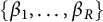 $\{\beta _1,\dots , \beta _R\}$
be a maximal
 $\eta $
-separated subset of
 $[\varepsilon ,\tfrac {3}{4} - \varepsilon ]$
. Then, for each
 $\beta _i$
, we get a full-measure set
 $\Omega _i \subset [0,1]$
such that if
 $\alpha \in \Omega _i$
, the conclusion of Theorem 2.2 holds with
 $\beta = \beta _i$
and with
 $\eta $
as chosen. We claim that
 $\Omega = \cap _{i \leqslant R} \Omega _i$
is a suitable full-measure set of values of
 $\alpha $
in Theorem 2.1.
Indeed, let
 $\alpha \in \Omega $
and let
 $s_1,t_1,s_2,t_2 \in \mathbb {R}$
with
 $s_1 < t_1$
and
 $s_2 < t_2$
. From Theorem 2.2, we know that, for all
 $i \leqslant R$
, for any
 $\delta>0$
, for all
 $N \geqslant N_0(\alpha ,\beta _i,\eta , \delta , \mathbf {s},\mathbf {t})$
, and for any L in the range
 $N^{1 - \beta _i - \eta } < L < N^{1 - \beta _i + \eta }$
, we have
 $$ \begin{align} \vert R_3(\alpha,L,N,g_{\mathbf{s},\mathbf{t}}) - L^2(t_1 - s_1)(t_2 - s_2)\vert < \delta L^2. \end{align} $$
Now, given any N and any L in the range
 $N^{1/4 + \varepsilon } < L < N^{1 - \varepsilon }$
, there exists an i such that
 $N^{1 - \beta _i - \eta } < L < N^{1 - \beta _i + \eta }$
. Therefore, if
 $N \geqslant \max _{i\leqslant R} N_0(\alpha ,\beta _i,\eta , \delta , \mathbf {s},\mathbf {t})$
, the inequality (2.5) holds. Because
 $\delta $
is arbitrary, the conclusion of Theorem 2.1 holds.▪
3 Proof of Theorem 2.2
Our task is now to prove Theorem 2.2. Let us fix
 $\beta $
and
 $\eta $
, which is assumed to be sufficiently small, and for the time being, let us also fix some
 $\alpha \in [0,1]$
and some
 $s_1,t_1,s_2,t_2 \in \mathbb {R}$
with
 $s_1 < t_1$
and
 $s_2 < t_2$
. We may also assume, without loss of generality, that N is sufficiently large in terms of
 $\alpha $
,
 $\beta $
,
 $\eta $
,
 $\mathbf {s}$
, and
 $\mathbf {t}$
.
We begin by replacing
 $\alpha $
with a suitably good rational approximation
 $a/q$
. Assume that there exists some rational
 $a/q$
, with q prime, for which
 $$ \begin{align} \left\vert \alpha -\frac{a}{q} \right\vert \leqslant \frac{1}{q^{2-\eta}} \end{align} $$
and
 $$ \begin{align} N^{\frac{2 + \beta}{2} + 10\eta} \leqslant q \leqslant 2 N^{\frac{2 + \beta}{2} + 10\eta}. \end{align} $$
We will show in Section 4 that almost all
 $\alpha $
admit such an approximation. Then, for such a pair
 $(N,q)$
, we define
 $$ \begin{align} A(N,q,c_1,c_2): = \vert \{ x,y,z \leqslant N : x^2 - y^2 \equiv c_1 \, (\text{mod } q), \, y^2 - z^2 \equiv c_2 \, (\text{mod } q)\}\vert. \end{align} $$
We then claim that
 $$ \begin{align} \frac{1}{N}\sum\limits_{\substack{(r_1,r_2) \in S^- \\ r_1r_2 \neq 0 \\ r_1 + r_2 \neq 0}} A(N,q,\overline{a} r_1,\overline{a} r_2) &\leqslant R_3(\alpha, L,N,g_{\mathbf{s},\mathbf{t}}) \leqslant \frac{1}{N} \sum\limits_{\substack{(r_1,r_2) \in S^+ \\ r_1r_2 \neq 0 \\ r_1 + r_2 \neq 0}} A(N,q,\overline{a} r_1,\overline{a} r_2), \end{align} $$
where
 $\overline {a}$
denotes the inverse of a modulo q,
 $$ \begin{align} S^{-} = \left \{ (r_1,r_2) \in \mathbb{Z}^2: \frac{s_i qL}{N} + \frac{N^2}{q^{1- \eta}} \leqslant r_i \leqslant \frac{t_i qL}{N} - \frac{N^2}{q^{1- \eta}}, \, i = 1,2 \right\}, \end{align} $$
and
 $$ \begin{align} S^+ = \left \{ (r_1,r_2) \in \mathbb{Z}^2: \frac{s_i qL}{N} - \frac{N^2}{q^{1- \eta}} \leqslant r_i \leqslant \frac{t_i qL}{N} + \frac{N^2}{q^{1- \eta}}, \, i=1,2 \right \}. \end{align} $$
Indeed, given
 $x,y$
in the range
 $1 \leqslant x,y \leqslant N$
, let us consider
 $r_1 \in \mathbb {Z}$
to be defined by the relation
 $$ \begin{align*} a (x^2 - y^2) \equiv r_1 \, (\text{mod }q)\end{align*} $$
and
 $-q/2 < r_1 < q/2$
. Suppose that
 $$ \begin{align*} \frac{s_1 qL}{N} + \frac{N^2}{q^{1- \eta}} \leqslant r_1 \leqslant \frac{t_1 qL}{N} - \frac{N^2}{q^{1- \eta}}.\end{align*} $$
Then, we have the inequalities
 $$ \begin{align*} \{\alpha(x^2 - y^2) \}_{\operatorname{sgn}} \leqslant \left\{\frac{a}{q} (x^2 - y^2)\right\}_{\operatorname{sgn}} + \left\vert \left( \alpha - \frac{a}{q}\right)(x^2 - y^2)\right\vert \leqslant \frac{r_1}{q} + \frac{N^2}{q^{2-\eta}} \leqslant t_1 \frac{L}{N} \end{align*} $$
and
 $$ \begin{align*}\{\alpha(x^2 - y^2) \}_{\operatorname{sgn}} \geqslant \left\{\frac{a}{q} (x^2 - y^2)\right\}_{\operatorname{sgn}} - \left\vert \left( \alpha - \frac{a}{q}\right)(x^2 - y^2)\right\vert \geqslant \frac{r_1}{q} - \frac{N^2}{q^{2-\eta}} \geqslant s_1 \frac{L}{N}.\end{align*} $$
Suppose instead that
 $$ \begin{align*} s_1 \frac{L}{N} \leqslant \{ \alpha(x^2 - y^2)\}_{\operatorname{sgn}} \leqslant t_1 \frac{L}{N}.\end{align*} $$
Then, similarly to the above, we have
 $$ \begin{align*}r_1 = q \left\{\frac{a}{q}(x^2 - y^2)\right\}_{\operatorname{sgn}} \leqslant q\left(\{ \alpha(x^2 - y^2)\}_{\operatorname{sgn}} + \left\vert \left( \alpha - \frac{a}{q}\right)(x^2 - y^2)\right\vert\right) \leqslant t_1 \frac{Lq}{N} + \frac{N^2}{q^{1- \eta}} \end{align*} $$
and
 $$ \begin{align*}r_1 = q \left\{\frac{a}{q}(x^2 - y^2)\right\}_{\operatorname{sgn}} \geqslant q \left(\{ \alpha(x^2 - y^2)\}_{\operatorname{sgn}} - \left\vert \left( \alpha - \frac{a}{q}\right)(x^2 - y^2)\right\vert\right) \geqslant s_1 \frac{Lq}{N} - \frac{N^2}{q^{1- \eta}} . \end{align*} $$
Finally, take
 $1 \leqslant z \leqslant N$
and define
 $r_2$
by the relation
 $$ \begin{align*} a(y^2 - z^2) \equiv r_2 \, (\text{mod } q)\end{align*} $$
with
 $-q/2 < r_2 < q/2$
. Then, because
 $N < q/2$
, we have that
 $x,y,z$
are distinct if and only if
 $r_1r_2 \neq 0$
and
 $r_1 + r_2 \neq 0$
.
From all these observations taken together, claim (3.4) is settled.
Remark: The reader might find it helpful to note, at this early stage, that the relative sizes of N and q were chosen, so that the two terms
 $qL/N$
and
 $N^2/q^{1-\eta }$
which appear in (3.5) and (3.6) are of approximately the same magnitude, namely
 $q^{(2-\beta )/(2+\beta )}$
.
A substantial portion of this paper will involve estimating the quantity
 $A(N,q,c_1,c_2)$
, on average over
 $c_1$
and
 $c_2$
. To this end, we let
 $$ \begin{align*} A_0(q,c_1,c_2) = \vert \{ x,y,z \leqslant q: x^2 - y^2 \equiv c_1 \, (\text{mod } q), \, y^2 - z^2 \equiv c_2 \, (\text{mod } q)\}\vert\end{align*} $$
be the number of solutions to the key congruences, in which the variables
 $x,y,z$
may range over the entire field
 $\mathbb {Z}/q\mathbb {Z}$
. One might reasonably expect that
 $$ \begin{align*}A(M,q,c_1,c_2) \approx (M/q)^3 A_0(q,c_1,c_2)\end{align*} $$
as long as M is large enough, and so we introduce the difference
 $$ \begin{align} \Delta(M,q,c_1,c_2) : = \left\vert A(M,q,c_1,c_2) - \left(\frac{M}{q}\right)^3 A_0(q,c_1,c_2)\right\vert. \end{align} $$
The following key technical lemma will be proved in Section 5.
Lemma 3.1 If q is an odd prime and
 $M<q$
, then
 $$ \begin{align} \sum\limits_{c_1,c_2 \leqslant q} \Delta(M,q,c_1,c_2)^2 \ll (\log q)^3M^3 + (\log q)^6q^{2},\end{align} $$
as
 $q \rightarrow \infty $
.
Lemma 3.1 can be used, in turn, in Section 6 to prove the following lemma on the average size of the error terms
 $\Delta (N,q,\overline {a}r_1, \overline {a}r_2)$
, which is helpful for analyzing the relation (3.4).
Lemma 3.2 Let
 $\beta \in (0, \tfrac {3}{4})$
and let
 $\eta>0$
. Then, if
 $\eta \max (\beta ^{-1}, (\tfrac {3}{4} - \beta )^{-1})$
is small enough, the following holds: for almost all
 $\alpha \in [0,1]$
, for all
 $s_1,t_1,s_2,t_2 \in \mathbb {R}$
for which
 $s_1 < t_1$
and
 $s_2 < t_2$
, for all
 $N \in \mathbb {N}$
, and for all
 $L \in \mathbb {R}$
in the range
 $N^{1 - \beta - \eta }<L<N^{1- \beta + \eta }$
, and for all prime q and
 $a/q$
satisfying (3.1) and (3.2), we have
 $$ \begin{align} \frac{1}{N}\sum\limits_{\substack{(r_1,r_2) \in S^+ \\ r_1r_2 \neq 0 \\ r_1 + r_2 \neq 0}} \Delta(N,q,\overline{a}r_1, \overline{a}r_2) \ll_{\alpha, \beta, \eta,\mathbf{s},\mathbf{t}} L^2 q^{-\eta}, \end{align} $$
where
 $S^{+}$
is as defined in (3.6).
At this point, it is worth us taking a small diversion from the main proof to discuss the numerology in Lemma 3.1, and why the bound is close to best possible. We begin with an easy lemma concerning
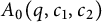 $A_0(q,c_1,c_2)$
itself. A more sophisticated version of this lemma was worked out by Rudnick and Kurlberg in [Reference Rudnick and Kurlberg22, Proposition 4], but to make our exposition self-contained, we decided to include a direct proof for the triple correlation case.
Lemma 3.3 Let q be an odd prime. If
 $c_1, c_2$
are not both divisible by q, then
 $$ \begin{align*} A_0(q,c_1,c_2) = \begin{cases} q + O(\sqrt{q}) & \text{if } c_1 + c_2 \not\equiv 0 \, (\text{mod }q), \\[2pt] 2q-1 - \left( \frac{-c_2}{q}\right) & \text{if } c_1 \equiv 0 \, (\text{mod } q),\\[2pt] 2q - 1 - \left( \frac{c_1}{q}\right) & \text{if } c_2 \equiv 0 \, (\text{mod } q), \\[2pt] 2q - 1 - \left(\frac{c_2}{q}\right) & \text{if } c_1 + c_2 \equiv 0 \, (\text{mod }q),\end{cases} \end{align*} $$
where
 $(\frac {\cdot }{q})$
denotes the Legendre symbol modulo q. Furthermore,
 $A_0(q,0,0)=4q-3$
.
Remark: For this paper, it would have been enough to consider only the nondegenerate case of Lemma 3.3. However, the arguments of Section 5 are cleaner if we allow ourselves to include the degenerate cases, which is the reason why we do so.
Proof In the trivial case
 $c_1\equiv c_2 \equiv 0 \,(\text {mod }q)$
, we note that
 $y=\pm x \,(\text {mod }q)$
and
 $z= \pm y \,(\text {mod }q)$
. So, except for when
 $x=q$
, there are four choices for
 $y,z$
given a fixed x, thus showing that
 $A_q(0,0) = 4(q-1) + 1 = 4q-3$
as claimed.
Thus, we assume in the following that at least one of
 $c_1,c_2$
is not divisible by q. We have that
 $$ \begin{align*} A_0(q,c_1,c_2) &= \frac{1}{q^2}\sum\limits_{\substack{0 \leqslant j,k \leqslant q-1 \\ 0\leqslant x,y,z \leqslant q-1}}e_q(j(x^2 - y^2 - c_1) + k(y^2 - z^2 - c_2)). \end{align*} $$
The terms when
 $j = 0$
,
 $k=0$
, or
 $j=k$
contribute
 $$ \begin{align*} \frac{1}{q^2}\left(q^2 \sum\limits_{ \substack{0 \leqslant x,y \leqslant q-1 \\ y^2 \equiv x^2 - c_1 \, (\text{mod }q)}} 1 + q^2 \sum\limits_{ \substack{0 \leqslant y,z \leqslant q-1 \\ y^2 \equiv z^2 +c_2 \, (\text{mod }q)}} 1 + q^2 \sum\limits_{ \substack{0 \leqslant x,z \leqslant q-1 \\ x^2 = z^2 + c_1 + c_2}}1 - 2q^3\right), \end{align*} $$
where the final term is used to correct for the overcounting of
 $(j,k) = (0,0)$
. By factorizing the ranges of summation using the difference of two squares, this expression is equal to
 $$ \begin{align*} q + (q-1)(1_{q\vert c_1}+1_{q \vert c_2}+1_{q\vert(c_1+c_2)}).\end{align*} $$
Recall the Gauss sum evaluation
 $$ \begin{align} \sum\limits_{ 0 \leqslant x \leqslant q-1} e_q(j x^2) = \left(\frac{j}{q}\right) \varepsilon_q \sqrt{q}, \end{align} $$
when
 $q \nmid j$
and where
 $\varepsilon _q = 1$
if
 $q \equiv 1 \, (\text {mod }4)$
and
 $\varepsilon _q = i$
if
 $q \equiv 3 \, (\text {mod }4)$
(see [Reference Iwaniec and Kowalski13, Theorem 3.3]). Therefore, the contribution from the remaining frequencies
 $j,k$
is exactly
 $$ \begin{align*} \frac{\varepsilon_q^3}{q^{1/2}}\sum\limits_{ \substack{1 \leqslant j,k \leqslant q-1 \\ j \neq k}} \left( \frac{j}{q}\right) \left( \frac{k-j}{q}\right) \left(\frac{-k}{q}\right) e_q(-jc_1) e_q(-k c_2). \end{align*} $$
By introducing a change of variables
 $k = lj$
, this expression is equal to
 $$ \begin{align} \frac{\varepsilon_q^3}{q^{1/2}}\left(\frac{-1}{q}\right) \sum\limits_{ 2 \leqslant l \leqslant q-1} \left(\frac{l-1}{q}\right) \left( \frac{l}{q} \right) \sum\limits_{1 \leqslant j \leqslant q-1}\left(\frac{j}{q}\right) e_q(j(-c_1 - lc_2)). \end{align} $$
One can evaluate the inner sum of (3.11) using (3.10). Indeed, for an arbitrary integer m and an arbitrary quadratic nonresidue h, we have
 $$ \begin{align*} \sum\limits_{ 1 \leqslant j \leqslant q-1} \left(\frac{j}{q}\right) e_q(jm) &= \frac{1}{2}\left(\sum\limits_{1 \leqslant n \leqslant q-1} e_q(mn^2) - \sum\limits_{1 \leqslant n \leqslant q-1} e_q(mn^2h)\right)\\ & = \frac{1}{2}\left(\sum\limits_{0 \leqslant n \leqslant q-1} e_q(mn^2) - \sum\limits_{0 \leqslant n \leqslant q-1} e_q(mn^2h)\right) \\ &= \frac{1}{2}\left(\left(\frac{m}{q}\right) - \left(\frac{hm}{q}\right)\right)\varepsilon_q \sqrt{q}\\ & = \left(\frac{m}{q}\right) \varepsilon_q \sqrt{q}. \end{align*} $$
Plugging this expression into (3.11), we establish that (3.11) is equal to
 $$ \begin{align*} \sum\limits_{2 \leqslant l \leqslant q-1} \left(\frac{l(l-1)(lc_2 + c_1)}{q}\right). \end{align*} $$
This is
 $O(\sqrt {q})$
by Hasse (see [Reference Iwaniec and Kowalski13, equation (14.32)]), provided that neither
 $q \vert c_1$
,
 $q\vert c_2$
, nor
 $q \vert (c_1 + c_2)$
.
In the singular cases, if q divides
 $c_1$
, we end up with
 $$ \begin{align*}\left(\frac{c_2}{q}\right) \sum\limits_{ 2 \leqslant l \leqslant q-1} \left( \frac{l-1}{q}\right),\end{align*} $$
which is equal to
 $-(\frac {-c_2}{q}) $
. If
 $q \vert (c_1 + c_2)$
, we end up with
 $$ \begin{align*} \left(\frac{c_2}{q}\right) \sum\limits_{ 2 \leqslant l \leqslant q-1} \left(\frac{l}{q}\right),\end{align*} $$
which is equal to
 $- (\frac {c_2}{q})$
. The final case, when
 $q \vert c_2$
, follows easily from the case
 $q \vert c_1$
after permuting the variables
 $x,y,z$
in the original expression for
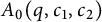 $A_0(q,c_1,c_2)$
.▪
Therefore,
 $(M/q)^3 A_0(q,c_1,c_2) \asymp M^3 q^{-2}$
, and this is the expected size of
 $A(M,q,c_1,c_2)$
. We note, then, that the
 $M^3$
term in (3.8) represents “square-root cancellation on average” for the size of
 $\Delta (M,q,c_1,c_2)$
.
Moreover, Lemma 3.1 is close to best possible, at least for certain ranges of M. We would like to emphasize that here and throughout, M denotes a positive integer. Indeed, if
 $M < \lambda q^{2/3}$
and
 $\lambda $
is a suitably small constant, then we have the matching lower bound
 $$ \begin{align} \sum\limits_{c_1,c_2 \leqslant q} \Delta(M,q,c_1,c_2)^2 \gg M^3. \end{align} $$
Proof Certainly,
 $$ \begin{align*} \sum\limits_{c_1,c_2 \leqslant q} A(M,q,c_1,c_2) = M^3.\end{align*} $$
Furthermore,
 $$ \begin{align*} \sum\limits_{c_1,c_2 \leqslant q} A(M,q,c_1,c_2)^2 = \sum\limits_{\substack{x,y,z,x^\prime,y^\prime,z^\prime \leqslant M\\ x^2 - (x^\prime)^2 \equiv y^2 - (y^\prime)^2 \equiv z^2 - (z^\prime)^2 \, (\text{mod }q)}} 1.\end{align*} $$
By using the divisor bound to control the terms arising when
 $x^2 - (x^\prime )^2 \neq 0$
, this sum is at most
 $O(q^{o(1)}M^2 q^{-1} + M^3)$
, which is certainly at most
 $O(M^3)$
.
Therefore, by Cauchy–Schwarz,
 $$ \begin{align*}\sum\limits_{c_1,c_2 \leqslant q} 1_{A(M,q,c_1,c_2) \geqslant 1} \geqslant \left(\sum\limits_{c_1,c_2 \leqslant q} A(M,q,c_1,c_2) \right)^2\left(\sum\limits_{c_1,c_2 \leqslant q} A(M,q,c_1,c_2)^2 \right)^{-1} \gg M^3.\end{align*} $$
If
 $Mq^{-2/3}$
is sufficiently small, then
 $(M/q)^3A_0(q,c_1,c_2) < \tfrac {1}{2}$
for all
 $c_1,c_2$
. Hence,
 $$ \begin{align*} \sum\limits_{ c_1,c_2 \leqslant q} \Delta(M,q,c_1,c_2)^2 \gg \sum\limits_{c_1,c_2 \leqslant q} 1_{A(M,q,c_1,c_2) \geqslant 1} \gg M^3\end{align*} $$
as claimed.▪
Rudnick, Sarnak, and Zaharescu [Reference Rudnick, Sarnak and Zaharescu24] also considered
 $\Delta (M,q,c_1,c_2)$
. By Fourier-expanding the cutoff
 $x,y,z \leqslant M$
, they derived
 $$ \begin{align*} \Delta(M,q,c_1,c_2) &\leqslant \sum\limits_{ \substack{0 \leqslant b_1,b_2,b_3 \leqslant q-1 \\ \mathbf{b} \neq \mathbf{0}}} \prod\limits_{i=1}^3 \vert \widehat{1}_{[M]}(b_i)\vert \left\vert \sum\limits_{\substack{0 \leqslant x,y,z \leqslant q-1 \\ x^2 - y^2 \equiv c_1 \, (\text{mod } q) \\ y^2 - z^2 \equiv c_2 \, (\text{mod } q)}} e_q(b_1x + b_2y + b_3 z)\right\vert, \end{align*} $$
where
 $$ \begin{align} \widehat{1_{[M]}}(b) = \frac{1}{q} \sum\limits_{x \leqslant M} e_q(-bx). \end{align} $$
In expression (9.15) of [Reference Rudnick, Sarnak and Zaharescu24] they used the Weil bound,Footnote 5 ending up with a bound of
 $$ \begin{align} \Delta(M,q,c_1,c_2) \ll q^{1/2} (\log q)^3, \end{align} $$
in the nondegenerate cases. Comparing this result to Lemma 3.1, estimate (3.14) implies
 $$ \begin{align} \sum\limits_{c_1,c_2 \leqslant q} \Delta(M,q,c_1,c_2)^2 \ll q^{3 + o(1)}, \end{align} $$
which is weaker than Lemma 3.1. We note, therefore, that the proof of Lemma 3.1 must utilize the extra averaging in
 $c_1$
and
 $c_2$
in a critical way.
In the introduction, we promised to explain how the threshold
 $N^{3/5}$
in Theorem 1.7 arises from the arguments of [Reference Rudnick, Sarnak and Zaharescu24], and now seems to be an appropriate moment. Indeed, in order to analyze (3.4), it would be enough to show that
 $$ \begin{align*}\Delta(N,q,\overline{a} r_1,\overline{a}r_2) = o((N/q)^3A_0(q,\overline{a} r_1,\overline{a}r_2)),\end{align*} $$
because then one could replace
 $A(N,q,\overline {a} r_1,\overline {a}r_2)$
with
 $(N/q)^3A_0(q,\overline {a} r_1,\overline {a}r_2)$
(and then evaluate these latter terms explicitly using Lemma 3.3). Using the bound (3.14), this is only possible when
 $N^3 q^{-2}>q^{1/2}(\log q)^3$
, that is, provided that
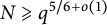 $N\geqslant q^{5/6 +o(1)}$
. This, one notes, is the same as the threshold from Theorem 4 of [Reference Rudnick, Sarnak and Zaharescu24] taken with
 $m=3$
(for triple correlations). Noting that
 $N \approx q^{\frac {2}{2+\beta }}$
, this approach succeeds provided that
 $2/(2+\beta )> 5/6$
, that is, provided that
 $\beta < 2/5$
. From the definition of
 $\beta $
, this implies that
 $ L$
must be at least
 $N^{3/5}$
.
Having finished our diversion on the subject of Lemma 3.1 (whose proof is deferred to Section 5), let us return to the main argument, namely the proof of Theorem 2.2. From now on, we assume
 $\alpha $
satisfies Lemma 3.2. Putting this information into expression (3.4), we derive
 $$ \begin{align} N^{2}q^{-3}\sum\limits_{\substack{ (r_1,r_2) \in S^{-} \\ r_1r_2 \neq 0 \\ r_1 + r_2 \neq 0}} A_0(q,\overline{a} r_1,\overline{a} r_2) - O_{\alpha,\beta,\eta, \mathbf{s}, \mathbf{t}}(L^2q^{-\eta}) \leqslant R_3^\prime(\alpha,L,N, g_{\mathbf{s},\mathbf{t}}) \nonumber \\ \leqslant N^{2}q^{-3} \sum\limits_{\substack{ (r_1,r_2) \in S^{+} \\ r_1r_2 \neq 0 \\ r_1 + r_2 \neq 0}}A_0(q,\overline{a} r_1,\overline{a} r_2) + O_{\alpha,\beta,\eta, \mathbf{s}, \mathbf{t}}(L^2q^{-\eta}) . \end{align} $$
To estimate the terms in the expression (3.16), we use Lemma 3.3. Indeed,
 $$ \begin{align} N^2 q^{-3} \sum\limits_{\substack{ (r_1,r_2) \in S^{\pm} \\ r_1r_2 \neq 0 \\ r_1 + r_2 \neq 0}}A_0(q,\overline{a} r_1,\overline{a} r_2) &= N^2 q^{-3} \sum\limits_{\substack{ (r_1,r_2) \in S^{\pm} \\ r_1r_2 \neq 0 \\ r_1 + r_2 \neq 0}} (q + O(q^{1/2})). \end{align} $$
The size of
 $S^{\pm }$
is given by
 $$ \begin{align*}\left( (t_1 - s_1) \frac{qL}{N} \pm 2 \frac{N^2}{q^{1-\eta}} + O(1)\right)\left( (t_2 - s_2) \frac{qL}{N} \pm 2 \frac{N^2}{q^{1-\eta}} + O(1)\right). \end{align*} $$
From relation (3.2), one observes that
 $$ \begin{align*}N^2 q^{-1 + \eta} = o_{\beta,\eta}\left(\frac{qL}{N}\right),\end{align*} $$
as
 $N \rightarrow \infty $
, and therefore, the size of
 $S^{\pm }$
is seen to be
 $$ \begin{align} \vert S^{\pm}\vert = (1+ o_{\beta,\eta, \mathbf{s}, \mathbf{t}}(1))(t_1 - s_1) (t_2 - s_2) q^2 L^2 N^{-2}, \end{align} $$
as
 $N \rightarrow \infty $
. The estimate (3.18) remains after we remove those pairs
 $(r_1,r_2) \in S^{\pm }$
with
 $r_1 r_2 = 0$
or
 $r_1 + r_2 = 0$
.
Thus, returning to (3.17), we conclude that
 $$ \begin{align*} N^2 q^{-3} \sum\limits_{\substack{ (r_1,r_2) \in S^{\pm} \\ r_1r_2 \neq 0 \\ r_1 + r_2 \neq 0}}A_0(q,\overline{a} r_1,\overline{a} r_2) = (1 + o_{\beta, \eta, \mathbf{s}, \mathbf{t}}(1))L^{2} (t_1 - s_1)(t_2 - s_2). \end{align*} $$
Substituting this estimate into (3.16), we derive Theorem 2.2 as required.▪
What remains is to verify that almost all
 $\alpha $
admit an approximation
 $a/q$
of the form required in (3.1) and (3.2), and to prove Lemmas 3.1 and 3.2.
4 Approximation with prime denominator
To derive a suitable approximation
 $a/q$
with prime denominator, we use the following quantitative version of (a generalized) Khintchine’s theorem, due to Harman.
Theorem 4.1 [Reference Harman11, Theorem 4.2]
Let
 $\psi :\mathbb {N}\rightarrow \left (0,1\right )$
be a nonincreasing function such that
 $$ \begin{align*}\Psi\left(N\right)=\sum_{n\leq N}\psi\left(n\right) \end{align*} $$
is unbounded. For
 $\mathcal {B}$
an infinite set of integers, let
 $S\left (\mathcal {B},\alpha ,N\right )$
denote the number of
 $n\leq N$
, with
 $n\in \mathcal {B}$
, such that
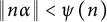 $\left \Vert n\alpha \right \Vert <\psi \left (n\right )$
. Then, for almost all
 $\alpha $
, we have
 $$ \begin{align} S\left(\mathcal{B},\alpha,N\right)=2\Psi(N,\mathcal{B})+O_{\varepsilon}(\left(\Psi(N)\right)^{\frac{1}{2}}(\log\Psi(N))^{2+\varepsilon}), \end{align} $$
for each
 $\varepsilon>0$
, where
 $$ \begin{align*}\Psi\left(N,\mathcal{B}\right)=\sum_{n\in\mathcal{B}\cap\left[N\right]}\psi\left(n\right).\end{align*} $$
Moreover, the implied constant in (4.1) is uniform in
 $\alpha $
.
From this, we deduce the following lemma.
Lemma 4.2 Let
 $\eta \in (0,1)$
. Then, for almost all
 $\alpha $
and for all
 $N \geqslant N_0(\eta )$
, there is a prime q satisfying
 $$ \begin{align} \left\Vert q\alpha\right\Vert <\frac{1}{N^{1-\eta}},\quad\mathrm{and}\quad N\leqslant q\leq2N. \end{align} $$
Proof We let
 $\mathcal {B}$
denote the set of primes, and
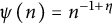 $\psi \left (n\right )=n^{-1+\eta }$
. Then,
 $\Psi (N) \sim \eta ^{-1}N^\eta $
and (by the prime number theorem)
 $\Psi (N,\mathcal {B}) \sim \eta ^{-1}N^{\eta }(\log N)^{-1}$
. So, the asymptotic formula (4.1) shows that, for almost all
 $\alpha $
, one has that
 $$ \begin{align*} S\left(\mathcal{B}, \alpha, N\right) & =\frac{2N^{\eta}\left(1+o\left(1\right)\right)}{\eta\log N}+O(\eta^{-1}N^{\frac{\eta}{2}}(\log N)^{3}), \end{align*} $$
with the implied constant uniform in
 $\alpha $
. From this, it immediately follows that if N is sufficiently large in terms of
 $\eta $
, then
 $$ \begin{align*}S(\mathcal{B},\alpha,2N) - S(\mathcal{B},\alpha,N)>0,\end{align*} $$
as required.▪
Therefore, an approximation
 $a/q$
may be found, with q prime, that satisfies (3.1) and (3.2).
5 Proof of Lemma 3.1
Expanding the square, we have
 $$ \begin{align*} \sum\limits_{c_1,c_2 \leqslant q} \Delta(N,q,c_1,c_2)^2 = S_1 - 2S_2 + S_3,\end{align*} $$
where
 $$ \begin{align*} S_1 &= \sum\limits_{c_1,c_2 \leqslant q} A(M,q,c_1,c_2)^2, \\ S_2 & = \left(\frac{M}{q}\right)^3\sum\limits_{c_1,c_2 \leqslant q} A(M,q,c_1,c_2) A_0(q,c_1,c_2), \\ S_3 & = \left(\frac{M}{q}\right)^6\sum\limits_{c_1,c_2 \leqslant q} A_0(q,c_1,c_2)^2. \end{align*} $$
We can write each
 $S_i$
as the number of solutions to certain equations, namely
 $$ \begin{align*} S_1& = \sum\limits_{\substack{1 \leqslant x,y,z \leqslant M \\ 1 \leqslant x^\prime, y^\prime, z^\prime \leqslant M \\ x^2 - y^2 \equiv (x^{\prime})^{2} - (y^{\prime})^{2} \, (\text{mod } q) \\ y^2 - z^2 \equiv(y^{\prime})^2 - (z^{\prime})^2 \, (\text{mod } q)}} 1 ,\\ S_2& = \left(\frac{M}{q}\right)^3\sum\limits_{\substack{1 \leqslant x,y,z \leqslant M \\ 1\leqslant x^\prime, y^\prime, z^\prime \leqslant q \\ x^2 - y^2 \equiv (x^{\prime})^{2} - (y^{\prime})^{2}\, (\text{mod } q) \\ y^2 - z^2 \equiv(y^{\prime})^2 - (z^{\prime})^2\, (\text{mod } q)}} 1 ,\\ S_3& = \left(\frac{M}{q}\right)^6 \sum\limits_{\substack{1 \leqslant x,y,z \leqslant q \\ 1 \leqslant x^\prime, y^\prime, z^\prime \leqslant q \\ x^2 - y^2 \equiv (x^{\prime})^{2} - (y^{\prime})^{2} \, (\text{mod } q)\\ y^2 - z^2 \equiv (y^{\prime})^2 - (z^{\prime})^2 \, (\text{mod } q)}} 1 . \end{align*} $$
Expanding the cutoffs
 $1 \leqslant x,y,z, x^\prime , y^\prime , z^\prime \leqslant M$
in terms of additive characters, we have
 $$ \begin{align*} S_1 = \sum\limits_{ \substack{ \mathbf{b} = (b_1,b_2,b_3,b_4,b_5,b_6),\\ 0 \leqslant b_1,b_2,b_3,b_4,b_5,b_6 \leqslant q-1 }} S(\mathbf{b},q) \prod\limits_{i=1}^6 \widehat{ 1_{[M]}}(b_i),\end{align*} $$
where
 $$ \begin{align*}S(\mathbf{b},q) := \sum\limits_{\substack{x,y,z \leqslant q \\ x^\prime,y^\prime,z^\prime \leqslant q \\ x^2 - y^2 \equiv (x^{\prime})^{2} - (y^{\prime})^{2} \, (\text{mod } q) \\ y^2 - z^2 \equiv(y^{\prime})^2 - (z^{\prime})^2 \, (\text{mod } q)}} e_q(\mathbf{b} \cdot (x,y,z,x^\prime,y^\prime,z^\prime))\end{align*} $$
and
 $\widehat {1_{[M]}}$
is as in (3.13). The contribution from the term with
 $\mathbf {b} = \mathbf {0}$
is equal to
 $S_3$
. Performing the same expansion on
 $S_2$
, we see that the terms arising from
 $\mathbf {b} = \mathbf {0}$
cancel, and we are left with the bound
 $$ \begin{align} S_1 - 2S_2 + S_3 \leqslant \sum\limits_{ \substack{ 0 \leqslant b_1,b_2,b_3,b_4,b_5,b_6 \leqslant q-1 \\ \mathbf{b} \neq \mathbf{0}}} \left(\prod\limits_{i=1}^6\vert \widehat{1_{[M]}}(b_i)\vert\right) \vert S(\mathbf{b},q)\vert. \end{align} $$
Our task moves to bounding
 $\vert S(\mathbf {b},q)\vert $
. We have the trivial bound
 $$ \begin{align*} \vert S(\mathbf{b},q)\vert \leqslant q^6,\end{align*} $$
but because q is prime and
 $\mathbf {b} \neq \mathbf {0}$
, we will be able to improve on this bound substantially.
Our approach will be elementary. We begin with writing
 $$ \begin{align} S(\mathbf{b},q) = \frac{1}{q^2} \sum\limits_{ j,k \leqslant q}\sum\limits_{\substack{x,y,z \leqslant q \\ x^\prime,y^\prime,z^\prime \leqslant q }} e_q(&\mathbf{b} \cdot (x,y,z,x^\prime,y^\prime,z^\prime) \nonumber \\&+ j(x^2 - y^2 - (x^\prime)^2 + (y^\prime)^2) \nonumber \\& + k (y^2 - z^2 - (y^\prime)^2 + (z^\prime)^2)). \end{align} $$
As we did when estimating
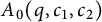 $A_0(q,c_1,c_2)$
, let us first consider the contribution from those terms when
 $j = 0$
,
 $k=0$
, or
 $j=k$
. This is
 $$ \begin{align} &\frac{1}{q^2} \sum\limits_{ k \leqslant q } \sum\limits_{\substack{x,y,z \leqslant q \\ x^\prime,y^\prime,z^\prime \leqslant q}} e_q(\mathbf{b} \cdot (x,y,z,x^\prime,y^\prime,z^\prime) + k(y^2 - z^2 - (y^\prime)^2 + (z^\prime)^2))\nonumber \\ & \quad + \frac{1}{q^2} \sum\limits_{ j \leqslant q } \sum\limits_{ \substack{x,y,z \leqslant q \\ x^\prime,y^\prime,z^\prime \leqslant q}} e_q(\mathbf{b} \cdot (x,y,z,x^\prime,y^\prime,z^\prime) + j(x^2 - y^2 - (x^\prime)^2 + (y^\prime)^2)) \nonumber\\ & \quad + \frac{1}{q^2} \sum\limits_{ j \leqslant q } \sum\limits_{\substack{x,y,z \leqslant q \\ x^\prime,y^\prime,z^\prime \leqslant q}} e_q(\mathbf{b} \cdot (x,y,z,x^\prime,y^\prime,z^\prime) + j(x^2 - z^2 - (x^\prime)^2 + (z^\prime)^2)) \nonumber\\ & \quad - \frac{2}{q^2}\sum\limits_{\substack{x,y,z \leqslant q \\ x^\prime,y^\prime,z^\prime \leqslant q}} e_q(\mathbf{b} \cdot (x,y,z,x^\prime,y^\prime,z^\prime)). \end{align} $$
The first three of these terms devolve into the exponential sums involved in the pair correlations of the fractional parts of
 $\alpha n^2$
considered by Heath-Brown in [Reference Heath-Brown12]. Indeed, note that, by completing the square in the variables
 $y, y^\prime , z, z^\prime $
, we have
 $$ \begin{align} \frac{1}{q^2}\sum\limits_{ k \leqslant q } \sum\limits_{\substack{x,y,z \leqslant q \\ x^\prime,y^\prime,z^\prime \leqslant q}} e_q(\mathbf{b} \cdot (x,y,z,x^\prime,y^\prime,z^\prime) + k(y^2 - z^2 - (y^\prime)^2 + (z^\prime)^2)) \end{align} $$
is equal to
 $$ \begin{align*}1_{q \vert b_1} 1_{q \vert b_4} \sum\limits_{ k \leqslant q-1} \vert G(k)\vert^4 e_q\left(\frac{-b_2^2 + b_3^2 + b_5^2 - b_6^2}{4k}\right), \end{align*} $$
where
 $$ \begin{align*} G(k) = \sum\limits_{ x \leqslant q} e_q(k x^2)\end{align*} $$
is the Gauss sum, as before, and
 $1_{q \vert b}$
abbreviates the indicator function of the condition
 $q\mid b$
. We also use
 $\frac {1}{k}$
to refer to the multiplicative inverse of k modulo q. Because
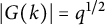 $\vert G(k)\vert = q^{1/2}$
by the standard evaluation (3.10), the term (5.4) is equal to
 $$ \begin{align} \begin{cases} q^3 - q^2 & \text{if } q \vert b_1, q \vert b_4, q \vert (-b_2^2 + b_3^2 + b_5^2 - b_6^2), \\ -q^2 & \text{if } q\vert b_1, q \vert b_4, q \nmid (-b_2^2 + b_3^2 + b_5^2 - b_6^2), \\ 0 & \text{if } q \nmid b_1 \text{ or } q \nmid b_4. \end{cases} \end{align} $$
We compute that the overall size of (5.3) is
 $$ \begin{align} \begin{cases} O(q^3) & \text{if } q\vert b_1, q \vert b_4, q \vert (-b_2^2 + b_3^2 + b_5^2 - b_6^2), \\ O(q^3) & \text{if } q\vert b_2, q \vert b_5, q \vert (-b_3^2 + b_1^2 + b_6^2 - b_4^2), \\ O(q^3) & \text{if } q\vert b_3, q \vert b_6, q \vert (-b_1^2 + b_2^2 + b_4^2 - b_5^2),\\ O(q^2) & \text{otherwise}. \end{cases} \end{align} $$
Now, consider the contribution to (5.2) when
 $j \neq 0$
,
 $k \neq 0$
, and
 $j \neq k$
. By completing the square again, this contribution is equal to
 $$ \begin{align} \frac{1}{q^2} \sum\limits_{\substack{j,k \leqslant q-1 \\ j \neq k}} \vert & G(j)\vert ^2\vert G(k-j)\vert ^2 \vert G(-k)\vert^2 \nonumber \\& \cdot e_{q}\left(-\frac{b_1^2}{4j} - \frac{b_2^2}{4(k-j)} - \frac{b_3^2}{4k}+\frac{b_4^2}{4j} + \frac{b_5^2}{4(k-j)} + \frac{b_6^2}{4k}\right). \end{align} $$
This is equal to
 $$ \begin{align*} q \sum\limits_{\substack{j,k \leqslant q-1 \\ j \neq k}}e_q\left( \frac{f(j,k)}{g(j,k)}\right), \end{align*} $$
where
 $$ \begin{align*} f(j,k) = j^2 (b_3^2 - b_6^2) + jk(b_1^2 - b_2^2 - b_3^2 - b_4^2 + b_5^2 + b_6^2) + k^2 (-b_1^2 + b_4^2) \end{align*} $$
and
 $$ \begin{align*} g(j,k) = 4 jk(-j+k).\end{align*} $$
By letting
 $l = j/k \, (\text {mod } q)$
, we can reparameterize this exponential sum as
 $$ \begin{align} q \sum\limits_{\substack{k \leqslant q-1 \\ 2 \leqslant l \leqslant q-1}} e_q\left(-\frac{f(l,1)}{k g(l,1)}\right). \end{align} $$
This, in turn, is equal to
 $$ \begin{align} q(q-1)R - q(q-2-R), \end{align} $$
where R is the number of
 $\ell $
in the range
 $2 \leqslant \ell \leqslant q-1$
for which
 $f(\ell ,1) = 0 \, (\text {mod } q)$
. There are two relevant cases. If
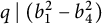 $q\mid (b_1^2 - b_4^2)$
,
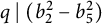 $q \mid (b_2^2 - b_5^2)$
, and
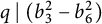 $q \mid (b_3^2 - b_6^2)$
, then
 $R = q-2$
, and so (5.9) is exactly equal to
 $q(q-1)(q-2)$
. Otherwise,
 $f(\ell ,1)$
is a nonzero polynomial of degree at most two in
 $\ell $
, and so
 $R = O(1)$
. Hence, (5.9) is
 $O(q^2)$
.
If we combine our knowledge of the sum (5.8) with our knowledge of the terms with
 $j=0,k=0,j=k$
from (5.6), this yields:
 $$ \begin{align} \vert S(\mathbf{b},q)\vert = \begin{cases} O(q^3) & \text{if } q\vert b_1, q \vert b_4, q \vert (-b_2^2 + b_3^2 + b_5^2 - b_6^2),\\ O(q^3) & \text{if } q\vert b_2, q \vert b_5, q \vert (-b_3^2 + b_1^2 + b_6^2 - b_4^2),\\ O(q^3) & \text{if } q\vert b_3, q \vert b_6, q \vert (-b_1^2 + b_2^2 + b_4^2 - b_5^2),\\ O(q^3) & \text{if } q \text{ divides all of } (b_1^2 - b_4^2), (b_2^2 - b_5^2), \text{ and } (b_3^2 - b_6^2),\\ O(q^2) & \text{otherwise.}\end{cases} \end{align} $$
Plugging this bound into (5.1), we infer that
 $$ \begin{align} S_1-2S_2+S_3 \ll q^3 (T_1 + T_2 ) + q^2 T_3, \end{align} $$
where (after a straightforward relabeling of the variables)
 $$ \begin{align*} T_1 = \sum\limits_{ \substack{ -q/2 < b_1,b_2,b_3,b_4,b_5,b_6 <q/2 \\ q\vert b_1 \pm b_4, q\vert b_2 \pm b_5, q \vert b_3 \pm b_6 \\ \mathbf{b} \neq \mathbf{0}}} \left(\prod\limits_{i=1}^6\vert \widehat{1_{[M]}}(b_i)\vert\right), \\ T_2 = \sum\limits_{ \substack{ -b/2 < b_1,b_2,b_3,b_4< q/2 \\ q \mid b_1^2 -b_2^2+b_3^2-b_4^2 \\ \mathbf{b} \neq \mathbf{0}}} \frac{M^2}{q^2} \left(\prod\limits_{i=1}^4\vert \widehat{1_{[M]}}(b_i)\vert\right),\\ T_3 = \sum\limits_{ \substack{ -q/2 < b_1,b_2,b_3,b_4,b_5,b_6 \leqslant q/2 \\ \mathbf{b} \neq \mathbf{0}}} \left(\prod\limits_{i=1}^6\vert \widehat{1_{[M]}}(b_i)\vert\right). \end{align*} $$
Indeed, because q is prime, if
 $q \vert b_1^2 - b_4^2$
, then
 $q\vert (b_1 + b_4)$
or
 $q \vert (b_1 - b_4)$
. This is one of the places in which the assumption that q is prime is particularly convenient (the other being the reparameterization of j and k to get (5.8)).
For
 $-q/2 < b < q/2$
, recall the standard bound
 $$ \begin{align*} \vert \widehat{1_{[M]}}(b)\vert \ll \min \left( \frac{M}{q}, \frac{1}{\vert b\vert}\right), \end{align*} $$
which produces the estimate
 $$ \begin{align*}\sum_{-q/2 < b < q/2} \vert \widehat{1_{[M]}}(b)\vert \ll \sum_{ \vert b \vert < q/M} \frac{M}{q} + \sum_{ q/M \leqslant \vert b \vert < q/2} \frac{1}{\vert b\vert} \ll \log q. \end{align*} $$
In the sum defining
 $T_1$
, if
 $(b_1,b_2,b_3)$
are fixed, then there are
 $O(1)$
possibilities for
 $(b_4,b_5,b_6)$
. Similarly, in
 $T_2$
, once
 $(b_1,b_2,b_3)$
are fixed, then there are at most two possibilities for
 $b_4$
. Hence,
 $$ \begin{align*}T_1,T_2 \ll \frac{M^3}{q^3} (\log q)^3 \quad \text{and}\quad T_3\ll (\log q)^6,\end{align*} $$
because
 $M<q$
. Substituting these bounds into (5.11), the proof of Lemma 3.1 is complete.▪
6 Proof of Lemma 3.2
Let
 $\beta $
and
 $\eta $
be as in the statement of Lemma 3.2. We begin the proof with another auxiliary lemma, which concerns the quantity
 $$ \begin{align*} \Delta^*_\beta( q, c_1,c_2) = \max_{M \leqslant q^{\frac{2}{2+\beta}}}\vert \Delta(M,q,c_1,c_2)\vert.\end{align*} $$
Lemma 6.1 Let q be an odd prime. Then, we have
 $$ \begin{align*}\sum\limits_{c_1,c_2\leqslant q} \Delta^*_\beta(q,c_1,c_2)^2 \ll q^{o(1)} q^{\frac{7 - \beta}{2+\beta}}.\end{align*} $$
Proof We will deduce this result from Lemma 3.1. Taking
 $1 \leqslant K \leqslant M \leqslant q$
, we begin by seeking a bound on
 $$ \begin{align} \sum\limits_{c_1,c_2 \leqslant q} (A( M+K, q,c_1,c_2) - A(M,q,c_1,c_2))^2. \end{align} $$
First,
 $A( M+K, q,c_1,c_2) - A(M,q,c_1,c_2)$
is at most
 $$ \begin{align*} &\vert \{ x \in (M,M+K],\, y,z \leqslant M+K : x^2 - y^2 \equiv c_1 \, (\text{mod } q), \, y^2 - z^2 \equiv c_2 \, (\text{mod } q)\}\vert \\ +&\vert \{ y \in (M,M+K], \, x,z \leqslant M+K: x^2 - y^2 \equiv c_1 \, (\text{mod } q), \, y^2 - z^2 \equiv c_2 \, (\text{mod } q)\}\vert \\ +&\vert \{ z \in (M,M+K], \, x,y \leqslant M+K: x^2 - y^2 \equiv c_1 \, (\text{mod } q), \, y^2 - z^2 \equiv c_2 \, (\text{mod } q)\}\vert. \end{align*} $$
Let
 $E_1(q,c_1,c_2)$
refer to the first quantity,
 $E_2(q,c_1,c_2)$
refer to the second quantity, and
 $E_3(q,c_1,c_2)$
refer to the third quantity. We have that expression (6.1) is at most a constant times
 $$ \begin{align*} \sum\limits_{c_1,c_2 \leqslant q}(E_1(q,c_1,c_2)^2 + E_2(q,c_1,c_2)^2 + E_3(q,c_1,c_2)^2).\end{align*} $$
By a change of variables, we may reduce consideration just to
 $E_2$
. Indeed, if
 $x^2 - y^2 \equiv c_1 \, (\text {mod }q)$
and
 $ y^2 - z^2 \equiv c_2 \, (\text {mod } q)$
, then
 $z^2-x^2 \equiv -c_1 -c_2 \, (\text {mod }q)$
. Hence,
 $E_1(q,c_1,c_2) = E_2(q,-c_1-c_2, c_1)$
, and so
 $$ \begin{align*}\sum\limits_{c_1,c_2 \leqslant q}E_1(q, c_1,c_2)^2 = \sum\limits_{c_1,c_2 \leqslant q} E_2(q, c_1,c_2)^2. \end{align*} $$
A similar argument works for
 $E_3(q,c_1,c_2)$
.
Now,
 $\sum _{c_1,c_2 \leqslant q}E_2(q,c_1,c_2)^2$
is equal to
 $$ \begin{align} \left\vert \left\{ y_1,y_2 \in (M,M+K],\, x_1,x_2,z_1,z_2 \leqslant M+K : \begin{array}{lr} x_1^2 - y_1^2 \equiv x_2^2 - y_2^2 (\text{mod } q),\\ y_1^2 - z_1^2 \equiv y_2^2 - z_2^2 \, (\text{mod } q) \end{array} \right\} \right\vert. \end{align} $$
Fixing integers
 $k_1,k_2$
and integers
 $y_1,y_2 \in (M,M+K]$
, we will now bound the number of solutions
 $(x_1,x_2,z_1,z_2)$
to the system of equations
 $$ \begin{align} x_1^2 - x_2^2 &= y_1^2 - y_2^2 + k_1 q, \nonumber\\ z_2^2 - z_1^2 & = y_2^2 - y_1^2 + k_2 q. \end{align} $$
If both
 $y_1 ^ 2 - y_2^2 + k_1q \neq 0$
and
 $y_2^2 - y_1^2 + k_2 q \neq 0$
then, using the divisor bound, we get
 $q^{o(1)}$
solutions. If
 $y_1 ^ 2 - y_2^2 + k_1q =0$
and
 $y_2^2 - y_1^2 + k_2 q \neq 0$
, we get
 $O(q^{o(1)}M)$
solutions. If both
 $y_1 ^ 2 - y_2^2 + k_1q =0$
and
 $y_2^2 - y_1^2 + k_2 q = 0$
, we get
 $O(M^2)$
solutions. Note that, in such a case, we must have
 $k_1 = -k_2$
.
Regarding the other conditions on
 $(y_1,y_2,k_1,k_2)$
, we note that the variables
 $k_1,k_2$
are both restricted to intervals of length
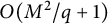 $O(M^2/q + 1)$
. Furthermore, if
 $k_1 \neq 0$
, then the total number of solutions of
 $y_1,y_2,k_1$
to
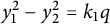 $y_1^2 - y_2^2 = k_1 q$
, with
 $y_1,y_2 \in (M, M+K]$
, is
 $O(q^{o(1)} (KM/q + 1))$
, because
 $\vert y_1^2 - y_2^2\vert = O(KM)$
. If, however,
 $k_1=0,$
then of course
 $y_1 = y_2$
, so there are
 $O(K)$
solutions here. Thus, summing over
 $(y_1,y_2,k_1,k_2)$
, we bound (6.2) above by
 $$ \begin{align*} &q^{o(1)}\Bigg(K^2\left(\frac{M^2}{q} + 1\right)^2 + M\left(\frac{M^2}{q} + 1\right)\left( \frac{KM}{q} + 1\right) + KM\left(\frac{M^2}{q} + 1\right)\\ &\quad + M^2\left(\frac{KM}{q} + 1\right) + K M^2\Bigg). \end{align*} $$
Because
 $K \leqslant M \leqslant q$
, we may simplify the above and conclude that
 $$ \begin{align} \sum\limits_{c_1,c_2 \leqslant q}(A(M+K,q,c_1,c_2) - A(M,q,c_1,c_2))^2 \ll q^{o(1)} (K^2 M^4 q^{-2} + KM^2). \end{align} $$
One may think of this upper bound as being given by the sum of an average contribution and a diagonal contribution.
From (6.4), together with previous lemmas, it turns out that one can control
 $$ \begin{align*} \sum\limits_{ 1 \leqslant c_1,c_2 \leqslant q} \max\limits_{0 \leqslant H \leqslant K} \Delta(M+H, q, c_1,c_2)^2.\end{align*} $$
Indeed, because
 $$ \begin{align*} \vert(a_1 - a_2)^2 - (b_1 - b_2)^2\vert \ll (a_1 - b_1)^2 + (a_2 - b_2)^2\end{align*} $$
for all reals
 $a_1,b_1,a_2,b_2$
, we have that
 $$ \begin{align} &\sum\limits_{c_1,c_2 \leqslant q} \max\limits_{0 \leqslant H \leqslant K}\Delta(M+H,q,c_1,c_2)^2 - \sum\limits_{ c_1,c_2 \leqslant q} \Delta(M,q,c_1,c_2)^2 \end{align} $$
is as most a constant times
 $$ \begin{align} \sum\limits_{c_1,c_2 \leqslant q} (A(M+K,q,c_1,c_2) &- A(M,q,c_1,c_2))^2 \nonumber\\ &+ \max\limits_{0 \leqslant H \leqslant K} \left(\frac{(M+H)^3-M^3}{q^3}\right)^2 \sum\limits_{c_1,c_2 \leqslant q} A_0(q,c_1,c_2)^2. \end{align} $$
From expression (6.4) and Lemma 3.3, we conclude that (6.6) is at most
 $$ \begin{align*} q^{o(1)}(K^2M^4q^{-2} + KM^2) \end{align*} $$
again. Finally, using Lemma 3.1 combined with (6.5), we end up with the bound
 $$ \begin{align} \sum\limits_{ c_1,c_2 \leqslant q} \max\limits_{0 \leqslant H \leqslant K}\Delta(M+H,q,c_1,c_2)^2 \ll q^{o(1)} (M^3 +q^2) + q^{o(1)}K^2M^4 q^{-2}. \end{align} $$
(The
 $KM^2$
term has been absorbed into the
 $M^3$
term.)
Before we use (6.7) to prove the lemma, we need the bound
 $$ \begin{align} \sum\limits_{c_1,c_2 \leqslant q} \max_{0 \leqslant H \leqslant K} \Delta(H,q,c_1,c_2)^2 \ll q^{o(1)}(K^6 q^{-2} + K^3). \end{align} $$
This may be proved by an identical analysis to the one above, proceeding with
 $M = 0$
.
Now, returning to the original object of the lemma, we may cover
 $$ \begin{align*}\{n \in \mathbb{N} : 1 \leqslant n \leqslant q^{\frac{2}{2+\beta}}\}\end{align*} $$
by the interval
 $[1,K]$
together with at most
 $q^{\frac {2}{2 + \beta }} K^{-1}$
other intervals, each of the form
 $[M,M+K]$
with
 $K \leqslant M$
. Thus,
 $$ \begin{align*} \sum\limits_{c_1,c_2 \leqslant q} \Delta^*_\beta(q,c_1,c_2)^2 &\leqslant q^{o(1)}(K^6q^{-2} + K^3) \\&\quad + \sum\limits_{l \leqslant q^{\frac{2}{2+\beta}}K^{-1}} \sum\limits_{ c_1,c_2 \leqslant q} \max\limits_{X \in [lK,(l+1) K)} \Delta(X,q,c_1,c_2)^2 \\ &\leqslant q^{o(1)}(K^6q^{-2} + K^3) + q^{o(1)}\sum\limits_{l \leqslant q^{\frac{2}{2+\beta}}K^{-1} } (l^3K^3+q^2 + l^4K^6 q^{-2}) \\ &\leqslant q^{o(1)}(K^6q^{-2} + K^3) + q^{o(1)} (q ^{\frac{8}{2+\beta}}K^{-1} + q^{\frac{2}{2+\beta} + 2}K^{-1} + q^{\frac{10}{2+\beta} - 2}K). \end{align*} $$
Because
 $\beta \leqslant 1$
always, we have
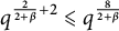 $q^{\frac {2}{2+\beta } + 2} \leqslant q^{\frac {8}{2 + \beta }}$
, which allows us to reduce matters to the bound
 $$ \begin{align*} q^{o(1)}(K^6 q^{-2} + K^3 + q^{\frac{8}{2+\beta}} K^{-1} + q^{\frac{10}{2+\beta} - 2}K).\end{align*} $$
Optimizing in K, we find that the minimum value is achieved when
 $K \asymp q^{\frac {1 + \beta }{2+\beta }}$
, in which case the third and fourth terms have the same order of magnitude. We conclude that
 $$ \begin{align*} \sum\limits_{c_1,c_2 \leqslant q} \Delta^*_\beta(q,c_1,c_2)^2 \ll q^{o(1)} q^{\frac{7 - \beta}{2+\beta}},\end{align*} $$
and the lemma is proved.▪
Proof of Lemma 3.2 Let C be a suitably large absolute constant. For all odd prime q, and integers a such that
 $(a,q) = 1$
, define
 $$ \begin{align} D_{\beta, \eta}(a,q) := \sum\limits_{ \substack{r_1,r_2 \neq 0 \\ \vert r_1\vert \leqslant q^{\frac{2-\beta}{2+\beta} + C\eta} \\ \vert r_2 \vert\leqslant q^{\frac{2-\beta}{2+\beta} + C\eta}}} \Delta^*_{\beta}(q, \overline{a} r_1,\overline{a}r_2). \end{align} $$
Now, suppose
 $\alpha \in [0,1]$
and fractions
 $a/q$
and N satisfy (3.1) and (3.2). We claim that, if C is large enough, and if q is large enough in terms of
 $\mathbf {s}$
,
 $\mathbf {t}$
, and
 $\eta $
, it follows that
 $$ \begin{align} \sum\limits_{\substack{ (r_1,r_2) \in S^+ \\ r_1r_2 \neq 0 \\ r_1 + r_2 \neq 0}} \Delta(N,q,\overline{a}r_1, \overline{a} r_2) \leqslant D_{\beta, \eta}(a,q). \end{align} $$
Indeed, because
 $N \leqslant q^{\frac {2}{2+\beta }}$
, we have
 $$ \begin{align*} \Delta(N,q, \overline{a} r_1, \overline{a}r_2) \leqslant \Delta^*_\beta(q,\overline{a} r_1, \overline{a}r_2).\end{align*} $$
In addition, we have both
 $$ \begin{align*}\frac{qL}{N} \ll N^{\frac{2+\beta}{2} - \beta + 11\eta} \ll q^{(\frac{2-\beta}{2} +11\eta)\frac{2}{2+\beta} + } \ll q^{\frac{2-\beta}{2+\beta} + C\eta}\end{align*} $$
and
 $$ \begin{align*}N^2 q^{\eta-1} \ll N^{2 - (1-\eta)(\frac{2+\beta}{2} + 10\eta)} \ll q^{(\frac{2-\beta}{2} + C\eta)\frac{2}{2+\beta} } \ll q^{\frac{2-\beta}{2+\beta} + C\eta}.\end{align*} $$
Referring to the definition (3.6) of
 $S^+$
, we have thus settled the inequality (6.10).
Therefore, to prove Lemma 3.2, it suffices to show that, for almost all
 $\alpha \in [0,1]$
, for all
 $(a,q,N)$
satisfying (3.1) and (3.2),
 $$ \begin{align} D_{\beta, \eta}(a,q)L^{-2}N^{-1} \ll_{\alpha,\beta,\eta} q^{-\eta}. \end{align} $$
In fact, by (3.2), it suffices to show that, for almost all
 $\alpha \in [0,1]$
and for all
 $(a,q)$
satisfying (3.1),
 $$ \begin{align} D_{\beta, \eta}(a,q) q^{\frac{-6 + 4 \beta}{2+\beta }} \ll_{\alpha,\beta, \eta} q^{-C\eta}. \end{align} $$
This expression makes no mention of N or L, which will be a technical necessity in the Borel–Cantelli argument to come.
To show (6.12), for each q, we define
 $$ \begin{align*} \operatorname{Bad}_{\beta, \eta}(q) = \{ a \leqslant q: (a,q) = 1, D_{\beta, \eta}(a,q)q^{\frac{-6 + 4 \beta}{2+\beta}}\geqslant q^{-C\eta}\}. \end{align*} $$
It will be enough, then, to show that, for almost all
 $\alpha \in [0,1]$
, only finitely many of the fractions
 $(a,q)$
satisfying (3.1) also satisfy
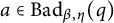 $a \in \operatorname {Bad}_{\beta , \eta }(q)$
.
To bound the size of
 $\operatorname {Bad}_{\beta , \eta }(q)$
, we first note that
 $$ \begin{align*}\vert \operatorname{Bad}_{\beta, \eta}(q)\vert \leqslant q^{\frac{-6 + 4 \beta}{2+\beta}+C\eta}\sum\limits_{ \substack{ 1 \leqslant a\leqslant q \\ (a,q) = 1}} D_{\beta, \eta}(a,q). \end{align*} $$
Furthermore, we define
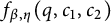 $f_{\beta , \eta }(q,c_1,c_2)$
to be the number of triples
 $(a,r_1,r_2)$
such that
 $$ \begin{align*} \overline{a} r_1 &\equiv c_1 \, (\text{mod }q), \\ \overline{a} r_2 &\equiv c_2 \, (\text{mod }q), \end{align*} $$
for which
 $1 \leqslant a \leqslant q$
,
 $(a,q) = 1$
,
 $r_1r_2 \neq 0$
, and
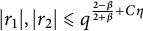 $\vert r_1\vert , \vert r_2\vert \leqslant q^{\frac {2-\beta }{2+\beta } + C\eta }$
. We then have
 $$ \begin{align} & \vert \operatorname{Bad}_{\beta, \eta}(q)\vert \leqslant q^{\frac{-6 + 4 \beta}{2+\beta } + C\eta} \sum\limits_{0 \leqslant c_1,c_2 \leqslant q-1} f_{\beta, \eta}(q,c_1,c_2) \Delta^*_\beta(q,c_1,c_2). \end{align} $$
To estimate (6.13), we need the following simple lemma about the size of
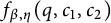 $f_{\beta , \eta }(q,c_1,c_2)$
.
Lemma 6.2 We have
 $$ \begin{align*}\sum\limits_{c_1,c_2 \leqslant q} f_{\beta, \eta}(q,c_1,c_2)^2 \ll q^{\frac{4 - 2 \beta}{2+\beta} + 2C\eta}(q + q^{\frac{4 - 2 \beta}{2+\beta} + 2C\eta })q^{o(1)}.\end{align*} $$
▪
Proof We have that
 $\sum _{c_1,c_2 \leqslant q} f_{\beta , \eta }(q,c_1,c_2)^2$
is equal to the number of pairs of triples
 $(a,r_1,r_2)$
,
 $(b,s_1,s_2)$
such that
 $$ \begin{align} \overline{a} r_1 &\equiv \overline{b} s_1 \, (\text{mod }q), \nonumber \\ \overline{a} r_2 &\equiv \overline {b} s_2 \, (\text{mod }q), \end{align} $$
with
 $1\leqslant a,b \leqslant q$
,
 $(a,q) = 1$
,
 $(b,q) = 1$
,
 $r_1r_2s_1s_2 \neq 0$
and
 $\vert r_1\vert , \vert r_2 \vert , \vert s_1\vert , \vert s_2\vert \leqslant q^{\frac {2-\beta }{2+\beta } + C\eta }$
. By multiplying the first equation by
 $br_2$
and the second equation by
 $br_1$
, one sees that, for every such solution, we must also have
 $$ \begin{align} s_1 r_2 \equiv s_2 r_1 \, (\text{mod } q). \end{align} $$
The mapping between the solutions to (6.14) and (6.15) is at most q-to-
 $1$
, because if the variables
 $a,r_1,r_2,s_1,s_2$
are fixed, then b is uniquely determined in (6.14).
Solutions to (6.15) are given by solutions
 $(r_1,r_2,s_1,s_2,k)$
to
 $$ \begin{align*} s_1r_2 - s_2r_1 = kq,\end{align*} $$
with k in the range
 $0 \leqslant \vert k\vert \ll q^{\frac {2(2-\beta )}{2+\beta } - 1 + 2C\eta }$
. By the divisor bound, after k,
 $s_1$
and
 $r_2$
are fixed there at most
 $q^{o(1)}$
valid choices of
 $s_2$
and
 $r_1$
, so the total number of solutions to (6.15) is at most
 $$ \begin{align*} q^{\frac{4 - 2\beta}{2+\beta} + 2 C\eta}(1 + q^{\frac{4-2\beta}{2+\beta} - 1 + 2C\eta}).\end{align*} $$
Multiplying by q to get the number of solutions to (6.14), we prove the lemma.▪
(The reader may wish to note that if
 $\beta>2/3$
, then the only valid value of k in the above is
 $k = 0$
, which simplifies the remainder of the analysis for these cases.)
Returning to (6.13), we have
 $$ \begin{align} \vert \operatorname{Bad}_{\beta, \eta}(q)\vert &\leqslant q^{\frac{-6 + 4 \beta}{2+\beta } + C\eta}\cdot \left(\sum\limits_{ c_1,c_2 \leqslant q} f_{\eta, \beta}(q,c_1,c_2)^2 \right)^{1/2}\cdot \left( \sum\limits_{c_1,c_2 \leqslant q} \Delta^*_\beta(q,c_1,c_2)^2 \right)^{1/2}\nonumber \\ & \ll q^{\frac{-6 + 4 \beta}{2+\beta }} \cdot (q^{\frac{1}{2} + \frac{2-\beta}{2+\beta}} + q^{\frac{4 - 2\beta}{2+\beta}}) \cdot q^{\frac{7 - \beta}{2(2+\beta)}}\cdot q^{C\eta + o(1)} \nonumber\\ &\ll (q^{\frac{1+6\beta}{2(2+\beta)}} + q^{\frac{3 + 3\beta}{2(2+\beta)}}) q^{C\eta + o(1)}. \end{align} $$
Here, we have used Lemmas 6.1 and 6.2 to go from the first line to the second line.
Now, recall that
 $\beta < \tfrac {3}{4}$
, which implies that
 $$ \begin{align*} \frac{ 1 + 6\beta}{2(2 + \beta)} < 1.\end{align*} $$
The other term is less severe, and, in fact,
 $\beta < 1$
implies
 $$ \begin{align*} \frac{3 + 3\beta}{2(2+ \beta)} < 1.\end{align*} $$
Because
 $\eta $
is small enough, and C is absolute, we conclude that
 $$ \begin{align} \vert \operatorname{Bad}(q,\beta,\eta) \vert \ll_{\beta,\eta} q^{1 - 2\eta}. \end{align} $$
Now, we can finally complete the proof of Lemma 3.2 by using the first Borel–Cantelli lemma. Indeed, pick
 $\alpha $
uniformly at random in
 $[0,1]$
, and for each prime
 $q \geqslant 3$
, let
 $E_{q,\beta , \eta }$
be the event that there exists an a with
 $1 \leqslant a \leqslant q$
,
 $(a,q) = 1$
,
 $$ \begin{align*}\left\vert \alpha - \frac{a}{q} \right\vert < \frac{1}{q^{2 - \eta}},\end{align*} $$
and
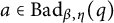 $a \in \operatorname {Bad}_{\beta , \eta }(q)$
. Then,
 $$ \begin{align*}\mathbb{P}(E_{q, \beta, \eta}) \leqslant \sum\limits_{ a \in \operatorname{Bad}_{\beta, \eta}(q)} \mu\left( \left(\frac{a}{q} - \frac{1}{q^{2-\eta}}, \frac{a}{q} + \frac{1}{q^{2 - \eta}}\right)\right) \ll_{\beta, \eta} q^{-1 -\eta}.\end{align*} $$
Then,
 $\sum _{q \geqslant 3} \mathbb {P}(E_{q, \beta , \eta }) < \infty $
, and so, with probability
 $1$
, only finitely many of the events
 $E_{q,\beta , \eta }$
occur. Thus, by our long chain of reductions, Lemma 3.2 follows.
7 Concluding remarks
The proof of all of our main theorems is now complete. However, before concluding the paper, it is certainly worth us discussing whether
 $\beta < \tfrac {3}{4}$
represents a natural limit of our approach.
The chain of inequalities (6.16) is the critical moment of the entire proof, and this particular application of Cauchy and Schwarz is the main source of our loss in the range of
 $\beta $
. Suppose that instead we had used the bound
 $$ \begin{align} \vert \operatorname{Bad}_{\beta, \eta}(q)\vert & \leqslant q^{\frac{-6 + 4 \beta}{2+\beta } + C\eta}\left( \sum\limits_{ c_1,c_2 \leqslant q} f_{\beta, \eta}(q,c_1,c_2)\right)^{1/2} \nonumber \\& \cdot \left(\sum\limits_{c_1,c_2 \leqslant q} f_{\beta, \eta}(q,c_1,c_2) \Delta^*_\beta(q,c_1,c_2)^2 \right)^{1/2}. \end{align} $$
For simplicity of exposition here, we will assume that
 $\beta> 2/3$
, that
 $C = 0$
, and we will ignore all
 $q^{o(1)}$
terms. It is then easy to see that
 $$ \begin{align*} \sum\limits_{c_1,c_2 \leqslant q} f_{\beta, \eta}(q,c_1,c_2) \approx q^{1 + \frac{2(2-\beta)}{2+\beta} }.\end{align*} $$
Combining this bound with Lemma 6.2, one may conclude that
 $f_{\beta , \eta }(q,c_1,c_2) \approx 1$
for
 $q^{1 + \frac {2(2-\beta )}{2+\beta }}$
pairs
 $(c_1,c_2)$
, and is
 $0$
otherwise. So, given what we know from Lemma 6.1 about the value of
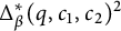 $\Delta ^*_\beta (q,c_1,c_2)^2$
averaged over all pairs
 $c_1$
and
 $c_2$
, it is not utterly unreasonable to hope that one could prove
 $$ \begin{align} \sum\limits_{c_1,c_2 \leqslant q} f_{\beta, \eta}(q,c_1,c_2) \Delta^*_\beta(q,c_1,c_2)^2 \ll_{\beta, \eta} q^{\frac{7 - \beta}{2+\beta}} \cdot q^{1 + \frac{2(2-\beta)}{2+\beta}} \cdot q^{-2}= q^{\frac{9 - 4\beta}{2 + \beta}}, \end{align} $$
provided that the weight of
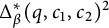 $\Delta ^*_\beta (q,c_1,c_2)^2$
does not concentrate on the support of f.
Putting this bound into (7.1), one would then get
 $$ \begin{align*}\vert \operatorname{Bad}_{\beta,\eta}(q)\vert \ll_{\beta, \eta} q^{\frac{3 + 3 \beta}{2(2+\beta)}},\end{align*} $$
that is, only the second term from (6.16) would occur. As we have already remarked, we would then derive
 $$ \begin{align*} \vert \operatorname{Bad}_{\beta, \eta}(q)\vert \ll_{\beta, \eta} q^{1- 2\eta},\end{align*} $$
provided
 $\beta < 1$
and
 $\eta $
is small enough. This estimate would expand the range of Theorem 1.4 all the way to
 $L> N^\varepsilon $
. Unfortunately, we have not been able to prove a version of Lemma 3.1, which includes the weight
 $f_{\beta , \eta }(q,c_1,c_2)$
in the manner of expression (7.2).
One also recalls that in our application of Borel and Cantelli, we did not need to bound
 $\vert \operatorname {Bad}_{\beta , \eta }(q)\vert $
uniformly for all q. One would be satisfied with
 $$ \begin{align*}\sum\limits_{q \text{ prime }}\frac{\vert \operatorname{Bad}_{\beta, \eta}(q)\vert}{q^2} < \infty.\end{align*} $$
Thoughts move toward expressing the relevant exponential sums as an average of Kloosterman-type sums over the modulus q, which might be another route for future research.
Our final remark is that if
 $L \rightarrow \infty $
and
 $N/L \rightarrow \infty $
as
 $N \rightarrow \infty $
, then, in the random model (1.4), the asymptotics are governed by the Central Limit Theorem. One can derive
 $$ \begin{align*}\frac{Z_{L,N} - L}{\sqrt{L}}\xrightarrow{dist} N(0,1),\end{align*} $$
as
 $N\rightarrow \infty $
. Theorem 1.4 could then be considered as a first step toward showing that, for almost all
 $\alpha $
, the skewness of
 $W_{\alpha ,L,N}$
satisfies
 $\mathbb {E} ((W_{\alpha ,L,N} - L)/\sqrt {L})^3\rightarrow 0$
as
 $N \rightarrow \infty $
, with L in a certain range. However, to show this asymptotic, one would need to be able to extract the lower degree main term from
 $\mathbb {E} W_{\alpha ,L,N}^3$
(which is
 $3L^2$
, as in Section 2), and then subsequently show that the error term in Theorem 2.1 is, in fact,
 $o(L^{3/2})$
, rather than merely
 $o(L^3)$
.
Appendix A Pair correlations of the dilated squares at scale
 $N^{-\beta }$

In this section, we briefly indicate how one can deduce the following fact from the methods of the literature.
Theorem A.1 Let
 $\varepsilon \in (0,\tfrac {1}{4})$
. Then, for almost all
 $\alpha \in [0,1]$
, for all
 $ 1\leqslant L \leqslant N^{1- \varepsilon }$
, and for all
 $(\log N)^{-1} \leqslant s \leqslant \log N$
, we have
 $$ \begin{align*}R_2(\alpha ,L, N, 1_{[-s,s]}) = 2Ls (1 + O_{\varepsilon,\alpha}(N^{-\varepsilon/13})). \end{align*} $$
Note that this result immediately implies the estimate (2.3), by approximating the function f in (2.3) with a suitable step function.
We have made no attempt to obtain the best possible error term in Theorem A.1, nor the largest admissible ranges for s and for L. One will observe from the proof that rather better bounds would certainly follow if one assumed at the outset that L were a slowly varying function of N.
A version of Theorem A.1 follows from arguments of Aistleitner, Larcher, and Lewko [Reference Aistleitner, Larcher and Lewko2] as well as from arguments of Rudnick [Reference Rudnick21] and Rudnick and Sarnak [Reference Rudnick and Sarnak23], by changing the relevant parameters. If one wanted an explicit characterization of the set of suitable
 $\alpha $
in terms of properties of its rational approximations, then one could also adapt the (much more involved) methods of Heath-Brown [Reference Heath-Brown12]. In particular, the material of the present section is in no way novel. However, we decided to add some explanations on how to deduce Theorem A.1, partly in order to make the exposition of our previous arguments complete and self-contained, and partly in order to describe explicitly a suitable “sandwiching argument” for this result (expanding upon the description in [Reference Aistleitner, Larcher and Lewko2]).
We begin with the following auxiliary lemma (where again no attempt was made to obtain the best possible error term).
Lemma A.2 For each
 $m \in \mathbb {N}$
, let
 $N_{m}=m^4$
. Letting
 $\varepsilon \in (0,\tfrac {1}{4})$
, for each i in the range
 $-m^{\varepsilon /3}/10 \leqslant i \leqslant m^{\varepsilon /3}$
, let
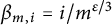 $\beta _{m,i} = i/m^{\varepsilon /3}$
and
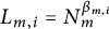 $L_{m,i} = N_m^{\beta _{m,i}}$
. Let
 $s_m$
be a real quantity that satisfies
 $ m^{-\varepsilon /10}<s_m < m^{\varepsilon /10}$
for large enough m. Then, for almost all
 $\alpha \in [0,1]$
, for all m, and for all i in the range
 $-m^{\varepsilon /3}/10 \leqslant i \leqslant m^{\varepsilon /3}$
, we have
 $$ \begin{align} R_2(\alpha,L_{m,i},N_m, 1_{[-s_m,s_m]}) = 2s_mL_{m,i} + O_{\alpha,\varepsilon}\left( \frac{L_{m,i}}{ m^{\frac{13}{15} - \frac{\varepsilon}{3}}}\right). \end{align} $$
Proof of Lemma A.2 Let
 $I=\left (\gamma ,\delta \right )$
be an arc on the torus
 $\mathbb {R}/ \mathbb {Z}$
such that
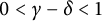 $0<\gamma -\delta <1$
. Let
 $J\geqslant 1$
be an integer. To proceed, we introduce trigonometric polynomials
 $S_{J}^{\pm }\left (x\right )$
, of degree J, which approximate the indicator function
 $\chi _{I}$
from above and below. Selberg, and also Vaaler, constructed such polynomials (cf. Montgomery [Reference Montgomery19, pp. 5–6]). Indeed, there exists
 $$ \begin{align*} S_{J}^{\pm}\left(x\right)= \sum_{\left|j\right|\leqslant J}s_{J}^{\pm}\left(j\right)e(jx), \end{align*} $$
satisfying
 $$ \begin{align*} S_{J}^{-}\left(x\right) \leqslant \chi_{I}\left(x\right) \leqslant S_{J}^{+}\left(x\right) \qquad(x\in\mathbb{R}/\mathbb{Z}), \end{align*} $$
such that
 $$ \begin{align*} s_{J}^{\pm}\left(0\right)=\delta - \gamma \pm\frac{1}{J+1}, \qquad\left|s_{J}^{\pm}\left(j\right)\right| \leqslant \frac{1}{J+1} +\min\left(\delta-\gamma,\frac{1}{\pi\left|j\right|}\right) \qquad\left(0<\left|j\right|\leqslant J\right). \end{align*} $$
For our purposes, given
 $N_m$
and some growth function
 $w(N_m) \geqslant 1$
, to be specified later, we specify
 $J_{m,i}= \lfloor N_mw(N_m)/L_{m,i} \rfloor $
,
 $\gamma _{m,i}=-s_mL_{m,i}/N_m$
, and
 $\delta _{m,i}=s_mL_{m,i}/N_m$
. Note that the definitions of
 $s_m$
and
 $L_{m,i}$
in the statement of the theorem imply that these choices yield a valid arc on the torus. Then, defining
 $$ \begin{align*} R_{2}^{\pm}(\alpha,L_{m,i},N_m,1_{[-s_m,s_m]}) :=\frac{1}{N_m}\sum_{x\neq y\leqslant N_m}S_{J_{m,i}}^{\pm}(\alpha(x^{2}-y^{2})), \end{align*} $$
we can control
 $R_{2}$
from above and below via
 $$ \begin{align} R_{2}^{-}(\alpha,L_{m,i},N_m,1_{[-s_m,s_m]}) & \leqslant R_{2}(\alpha,L_{m,i},N_m,1_{[-s_m,s_m]}) \nonumber \\& \leqslant R_{2}^{+}(\alpha,L_{m,i},N_m,1_{[-s_m,s_m]}). \end{align} $$
Let
 $$ \begin{align*} E^{\pm}(L_{m,i},N_m,s_m) := \int\limits_{0}^1 R_2^{\pm}(\alpha,L_{m,i},N_m,1_{[-s_m,s_m]}) \, d\alpha\end{align*} $$
be the expected value of
 $R_2^{\pm }(\alpha ,L_{m,i},N_m,1_{[-s_m,s_m]})$
. It is easy to see that
 $$ \begin{align} E^{\pm}(L_{m,i},N_m,s_m) = 2s_mL_{m,i}+ O(L_{m,i}/w(N_m)) + O(s_mL_{m,i}/N_m). \end{align} $$
Furthermore, by using orthogonality, we also see that the variance
 $$ \begin{align*} \int_{0}^{1} (R_{2}^{\pm}(\alpha,L_{m,i},N_m,1_{[-s_m,s_m]}) - E^{\pm}(L_{m,i},N_m,s_m))^2 d\alpha\end{align*} $$
of
 $R_2^{\pm }$
is at most
 $$ \begin{align*}\leqslant \frac{1}{N_m^2}\sum_{\substack{x_1\neq y_1 \leqslant N_m\\ x_2\neq y_2 \leqslant N_m}}\, \sum_{\substack{0< \vert j_1\vert,\vert j_2\vert \leqslant J_{m,i}\\ j_1(x_1^2 - y_1^2) + j_2 (x_2^2 -y_2^2) = 0}} \vert s_{J_{m,i}}^{\pm}(j_1) s_{J_{m,i}}^{\pm} (j_2) \vert.\end{align*} $$
(Note that there are no contributions from terms in which
 $j_1 = 0$
and
 $j_2 \neq 0$
, because the condition
 $j_2(x_2^2 - y_2^2) = 0$
cannot be satisfied.)
Because
 $\vert s_{J_{m,i}}^{\pm }(j) \vert \leqslant (2s_m + 1) L_{m,i}/N_m$
for all j in the range
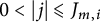 $0<\vert j\vert \leqslant J_{m,i}$
, we can bound the variance above by
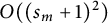 $O((s_m + 1)^2)$
times
 $$ \begin{align} \frac{L_{m,i}^2}{N_m^{4}} \left \vert \left\{(j_1,x_1,y_1,j_2,x_2,y_2) \in \mathbb{Z}^6 : \begin{array}{lr} j_1 (x_1^2 -y_1^2 ) = j_2 (x_2^2 -y_2^2 ),\\ 1\leqslant x_k\neq y_k \leqslant N_m,\\ 0 < \vert j_k \vert \leqslant \frac{N_m w(N_m)}{L_{m,i}},\\ k=1,2 \end{array} \right\} \right\vert. \end{align} $$
Let us fix the first three variables above, that is,
 $j_1,x_1,y_1$
. Then, by writing
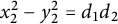 $x_2^2-y_2^2= d_1 d_2$
, with
 $d_1 = x_2-y_2$
and
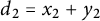 $d_2 = x_2+y_2$
, we deduce that
 $d_k \mid j_1 (x_1^2 -y_1^2 ) $
for
 $k = 1,2$
. By the divisor bound, there are at most
 $N_m^{o(1)}$
many possibilities for
 $d_1,d_2$
(provided that
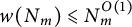 $w(N_m) \leqslant N_m^{O(1)}$
). Moreover, any choice of
 $d_1,d_2$
uniquely determines the variables
 $x_1,y_1$
via
 $ x_2 = (d_1 + d_2)/2 $
and
 $ y_2 = (d_2- d_1)/2 $
. Furthermore, we note that
 $j_2$
is determined up to
 $\ll N_m^{o(1)}$
many choices. The upshot is that given one of the
 $O( N_m^3 w(N_m)/L_{m,i})$
many admissible choices for
 $j_1,x_1,y_1$
, the second block of variables
 $j_2,x_2,y_2$
is determined up to
 $O(N_m^{o(1)})$
many possibilities. Therefore, the variance of
 $R_2^\pm $
is at most
 $O((s_m+1)^2L_{m,i} w(N_m) N_m^{-1 + o(1)})$
.
For the ease of exposition, we let
 $\kappa _{m,i}^{\pm }=\vert R_{2}^{\pm }(\alpha ,L_{m,i},N_{m},1_{[-s_m,s_m]}) - E^{\pm }(L_{m,i},N_m,s_m)\vert $
. We infer, by Chebychev’s inequality, that
 $$ \begin{align*} \mathbb{P} \left(\alpha\in\left[0,1\right]: \kappa_{m,i}^{\pm} \geqslant \frac{L_{m,i}}{w(N_m)} \right) \leqslant \frac{(s_m+1)^2w(N_m)^3 N_m^{o(1)}}{N_mL_{m,i}} \leqslant \frac{(s_m+1)^2w(N_m)^3 N_m^{o(1)}}{N_m^{9/10}}. \end{align*} $$
Choose the growth function
 $w(N_m)$
to be
 $$ \begin{align*} w(N_m) = \left(\frac{N_m^{9/10}}{m^{1 + \varepsilon}} \right)^{1/3}. \end{align*} $$
Therefore, because
 $s_m < m^{\varepsilon /10}$
, we conclude that
 $$ \begin{align*} \mathbb{P}\left(\alpha\in\left[0,1\right]: \kappa_{m,i}^{\pm}\geqslant \frac{L_{m,i}}{w(N_m)} \right) \ll_{\varepsilon} \frac{1}{m^{1 + \frac{\varepsilon}{2}}}. \end{align*} $$
Summing over i in the range
 $-m^{\varepsilon /3}/10 \leqslant i \leqslant m^{\varepsilon /3}$
, with the union bound, we get
 $$ \begin{align*} \mathbb{P}\left(\alpha\in\left[0,1\right]: \exists \, i \in [-m^{\varepsilon/3}/10, m^{\varepsilon/3}] \text{ s.t. } \kappa_{m,i}^{\pm} \geqslant \frac{L_{m,i}}{w(N_m)} \right) \ll_\varepsilon \frac{1}{m^{1 + \frac{\varepsilon}{6}}}. \end{align*} $$
Recalling our estimate (A.3), the first Borel–Cantelli lemma implies that, for almost every
 $\alpha \in \left [0,1\right ]$
, the following relation holds for all
 $m\geqslant 1$
and all admissible
 $i \in [-m^{\varepsilon /3}/10, m^{\varepsilon /3}]$
:
 $$ \begin{align*} \frac{1}{N_{m}}\sum_{x\neq y\leqslant N_{m}} R_2^{\pm}(\alpha,L_{m,i},N_m, 1_{[-s_m,s_m]}) = 2s_mL_{m,i} + O_{\alpha, \varepsilon}\left( \frac{L_{m,i}}{w(N_m)}\right) + O_{\alpha}\left(\frac{s_m}{N_m}\right). \end{align*} $$
From (A.2), and substituting in the explicit growth function
 $w(N_m)$
, the lemma follows.▪
Proof of Theorem A.1 We begin with the trivial observation that, by combining s and L into a single parameter, it is enough to show that, for almost all
 $\alpha \in [0,1]$
, for all N, and for all L in the range
 $ N^{-1/11}\leqslant L \leqslant N^{1 - \varepsilon /2}$
,
 $$ \begin{align} R_2(\alpha,L,N,1_{[-1,1]}) = 2L (1+ O_{\alpha,\varepsilon}(N^{-\frac{\varepsilon}{13}})). \end{align} $$
Now, for each N, choose m such that
 $N_{m}\leq N<N_{m+1}$
, where
 $N_m = m^4$
as in Lemma A.2. We put
 $\theta _{m}=N_{m+1}/N_{m}$
. Then, for any L,
 $$ \begin{align*} R_{2}(\alpha,L,N,1_{[-1,1]}) & \leqslant \frac{N_{m+1}}{N} R_{2}\left(\alpha,L,N_{m+1},1_{\frac{N_{m+1}}{N}[-1,1]}\right) \\ & \leqslant \theta_{m}R_{2}(\alpha,L,N_{m+1},1_{\theta_{m}[-1,1]}), \end{align*} $$
and similarly,
 $$ \begin{align*} R_{2}(\alpha,L,N,1_{[-1,1]}) \geqslant \frac{N_{m}}{N} R_{2}\left(\alpha,L,N_{m},1_{\frac{N_{m}}{N}[-1,1]}\right) \geqslant \theta_{m}^{-1}R_{2}(\alpha,L,N_{m},1_{\theta_{m}^{-1}[-1,1]}). \end{align*} $$
For each
 $ N^{-1/11}\leqslant L \leqslant N^{1 - \varepsilon /2}$
, there exists an i in the range
 $ - m^{\varepsilon /3}/10 \leqslant i\leqslant m^{\varepsilon /3}$
such that
 $L_{m,i} \leqslant L \leqslant L_{m,i+1}$
, where
 $L_{m,i}$
is as in Lemma A.2. Now, we record that the upper and lower bounds above satisfy
 $$ \begin{align*} & R_{2}(\alpha,L,N_{m},1_{\theta_{m}^{-1}[-1,1]}) \geqslant R_{2}(\alpha,L_{m,i},N_{m},1_{\theta_{m}^{-1}[-1,1]}),\\ & R_{2}(\alpha,L,N_{m+1},1_{\theta_{m}[-1,1]}) \leqslant R_{2}(\alpha,L_{m,i+1},N_{m+1},1_{\theta_{m}[-1,1]}). \end{align*} $$
Moreover, Lemma A.2 implies that there is a set
 $\Omega _{\varepsilon } \subset [0,1]$
, with full measure, such that, if
 $\alpha \in \Omega _{\varepsilon }$
and
 $\varepsilon \in (0,\tfrac {1}{4}]$
, then for all
 $m\geqslant 1$
and i in the range
 $ - m^{\varepsilon /3}/10 \leqslant i \leqslant m^{\varepsilon /3}$
,
 $$ \begin{align*} R_2(\alpha,L_{m,i},N_m, 1_{\theta_m[-1,1]}) = 2\theta_m L_{m,i}(1+ O_{\alpha,\varepsilon} (m^{-\frac{13}{15} + \frac{\varepsilon}{3}})).\end{align*} $$
By using that
 $ L_{m,i+1}/L_{m,i} = 1 + O_{\varepsilon }(N^{-\varepsilon /13})$
and also that
 $ \theta _{m}= 1+ O(m^{-1})$
, we infer that
 $$ \begin{align*} R_{2}(\alpha,L,N,1_{[-1,1]})& \leqslant 2L(1+ O_{\alpha,\varepsilon} (N^{-\frac{1}{4}})) (1+ O_{\alpha,\varepsilon}(N^{-\frac{\varepsilon}{13}}))(1 + O_{\alpha,\varepsilon}(m^{-\frac{13}{15} + \frac{\varepsilon}{3}})) \\ & \leqslant 2L(1 + O_{\alpha,\varepsilon}(N^{-\frac{\varepsilon}{13}})). \end{align*} $$
Similarly, we conclude that
 $$ \begin{align*}R_{2}(\alpha,L,N,1_{[-1,1]}) \geqslant 2 L(1+ O_{\alpha,\varepsilon}(N^{-\frac{\varepsilon}{13}})). \end{align*} $$
Combining these two estimates shows (A.5), thus completing the proof of Theorem A.1.▪
Appendix B Discrepancy and k-point correlation functions at scale
$N^{-\beta }$

The purpose of the present section is to record a few simple observations concerning the relationship between discrepancy and k-point correlation functions.
Definition B.1 Let
 $(x_n)_{n=1}^{\infty }$
be a sequence of points in
 $[0,1)$
. Let
 $k \geqslant 2$
be a natural number, and let
 $g: \mathbb {R}^{k-1} \longrightarrow [0,1]$
be a compactly supported function. Then, the kth correlation function
 $R_k((x_n)_{n=1}^\infty , L,N,g)$
is defined to be
 $$ \begin{align*}R_k((x_n)_{n=1}^\infty, L,N,g): = \frac{1}{N} \sum\limits_{\substack{n_1,\dots,n_k \leqslant N \\ \text{distinct}}} g\left(\frac{N}{L}y_1, \frac{N}{L} y_2, \dots, \frac{N}{L} y_{k-1}\right),\end{align*} $$
where
 $y_i = \{x_{n_i} - x_{n_{i+1}}\}_{\mathrm {sgn}}$
, for
 $i=1,\ldots ,k-1$
, with
 $$ \begin{align*} \{\cdot\}_{\mathrm{sgn}}:\mathbb{R} \longrightarrow (-1/2,1/2]\end{align*} $$
denoting the signed distance to the nearest integer.
The main point we are conveying here is that, as expected, the correlations are controlled on the scales in which the discrepancy allows us to count points asymptotically.
Lemma B.1 (a) Let
 $D_N$
denote the discrepancy of the sequence
 $(x_n)_{n=1}^\infty $
in
 $[0,1)$
, and suppose
 $\sup \{ g>0: D_N \ll _{g} N^{-g} \, \text {for all } N\} = \gamma > 0$
. Let
 $k \geqslant 2$
be a natural number, and let Y be a uniformly distributed random variable modulo
 $1$
. Let
 $\varepsilon> 0$
be suitably small in terms of
 $\gamma $
, and for all
 $N \in \mathbb {N}$
and
 $L \in \mathbb {R}$
satisfying
 $L \leqslant N$
, let
 $$ \begin{align*} W((x_n)_{n=1}^\infty,L,N): = \vert \{ n \leqslant N: x_n \in [Y,Y+L/N] \, \text{mod } 1 \}\vert.\end{align*} $$
Then, if L is in the range
 $N^{1 - \gamma + \varepsilon } < L \leqslant N$
, we have
 $$ \begin{align} \mathbb{E} W((x_n)_{n=1}^\infty,L,N)^k = L^k(1+O_{\varepsilon}(kN^{-\varepsilon/2})). \end{align} $$
Furthermore, for all continuous functions
 $g:\mathbb {R}^{k-1} \longrightarrow [0,1]$
and for all L in the range
 $N^{1 - \gamma + \varepsilon } < L < N^{1- \varepsilon }$
,
 $$ \begin{align} R_k((x_n)_{n=1}^\infty, L,N,g) = (1 + o_{g,\varepsilon,k}(1))L^{k-1}\int g(\mathbf{w}) \, d\mathbf{w}, \end{align} $$
as
 $N\rightarrow \infty $
, where the error term is independent of the choice of parameters L.
(b) If
 $(a_n)_{n=1}^\infty $
is a strictly increasing sequence of positive integers, for almost every
 $\alpha \in [0,1]$
, for all
 $N \in \mathbb {N}$
and for all
 $L \in \mathbb {R}$
in the range
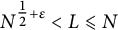 $N^{\tfrac {1}{2} + \varepsilon } < L \leqslant N$
, the sequence
 $$ \begin{align*}(\alpha a_n \text{ mod }1)_{n=1}^{\infty}\end{align*} $$
Remark: Part (b) of the lemma proves our earlier assertion (1.5).
Proof Fix a small
 $\varepsilon>0$
throughout this proof. For part (a), the proof of (B.1) is trivial. Indeed, by the discrepancy estimate, we have
 $$ \begin{align*} \vert \{n \leqslant N: x_n \in [Y,Y+L/N] \, \text{mod } 1\}\vert & = L + O(ND_N) \\ & = L + O_{\varepsilon}(N^{1 - \gamma + \varepsilon/2}) = L(1+O_{\varepsilon}(N^{- \varepsilon/2})). \end{align*} $$
Raising to the kth power and averaging over Y, we obtain (B.1).
To prove the correlation estimate (B.2), by approximating the function g by step functions, we see that it is enough to prove it in the case when g is the indicator function of a box
 $$ \begin{align*}[s_1,t_1] \times \dots \times [s_{k-1}, t_{k-1}].\end{align*} $$
We may assume, without loss of generality, that N is large enough, so that
 $(t_i - s_i)L/N \leqslant 1$
for all
 $i \leqslant {k-1}$
. (This is why it is important for the correlation estimate to preclude the case
 $L = N$
.) Then, fixing
 $n_k$
, we see that
 $R_k((x_n)_{n=1}^\infty , L,N,g)$
counts the number of
 $x_{n_{k-1}}\neq x_{n_k}$
such that
 $x_{n_{k-1}} \in [s_{k-1}L/N + x_{n_k}, t_{k-1} L/N + x_{n_k}] \, \text {mod } 1$
, times the number of
 $x_{n_{k-2}} \neq x_{n_{k-1}} ,x_{n_{k}}$
such that
 $x_{n_{k-2}} \in [s_{k-2}L/N + x_{n_{k-1}}, t_{k-2} L/N + x_{n_{k-1}}]\, \text {mod } 1$
, and so forth.
By the discrepancy estimate, the total number of choices is
 $$ \begin{align*} ((t_{k-1} - s_{k-1})L + O_{\varepsilon}(LN^{-\varepsilon/2})) & \times ((t_{k-2} - s_{k-2})L + O_{\varepsilon}(LN^{-\varepsilon/2})) \\ & \times \dots \times ((t_1 - s_1)L + O_{\varepsilon}(LN^{-\varepsilon/2})). \end{align*} $$
Summing over all
 $n_k$
and then normalizing by
 $1/N$
, we have
 $$ \begin{align*} R_k((x_n)_{n=1}^\infty, L, N, g) = \left( \prod\limits_{i=1}^{k-1} (t_i - s_i) \right) L^{k-1}(1 + O_{\varepsilon, g}(k N^{-\varepsilon/2})),\end{align*} $$
as desired.
This proves part (a) of the assertion. The remaining part follows by recalling that a classical (and far more general) result of Erdős and Koksma [Reference Erdős and Koksma9, Theorem 2] furnishes an upper bound on the discrepancy of
 $(\alpha a_n \text { mod }1)_{n=1}^{\infty }$
of the quality
 $N^{-1/2 + \varepsilon }$
, for each fixed
 $\varepsilon>0$
and for almost every
 $\alpha \in [0,1]$
.▪
Steinerberger [Reference Steinerberger27] raised the question of whether “most sequences”Footnote
6
have uniform pair correlations at some scale
 $0<\beta < 1$
. The above part (b) answers Steinerberger’s question in a strong sense. Furthermore, it seems worthwhile to record the following consequence. To state it, recall that for any irrational
 $\alpha \in [0,1]$
, there is a unique sequence of positive integers
 $\alpha _n \geq 1$
such that
 $$ \begin{align*} \alpha = \lim_{n \rightarrow \infty}\cfrac{1}{\alpha_1 + \cfrac{1}{\alpha_2 + \cfrac{1}{\ddots + \cfrac{1}{\alpha_n}}}}, \end{align*} $$
where
 $\alpha _n$
is called the nth partial quotient of
 $\alpha $
. Writing the fraction
 $$ \begin{align*}\cfrac{1}{\alpha_1 + \cfrac{1}{\alpha_2 + \cfrac{1}{\ddots + \cfrac{1}{\alpha_n}}}}=: \frac{p_n}{q_n}\end{align*} $$
in lowest terms, we call
 $q_n$
a convergent denominator of
 $\alpha $
.
Corollary B.2 Let
 $\alpha _n$
be the nth partial quotient of the irrational number
 $\alpha \in [0,1]$
. Given
 $N\geqslant 1$
, let
 $i(N)$
be such that the convergent denominator
 $q_{i(N)}$
of
 $\alpha $
satisfies
 $q_{i(N)} \leqslant N < q_{i(N)+1}$
. If, for each
 $\varepsilon>0$
, we have
 $$ \begin{align*}A_{N}(\alpha) =\sum_{j \leqslant i(N)} \alpha_{j} \ll N^{\varepsilon},\end{align*} $$
then the Kronecker sequence
 $(\alpha n)_{n=1}^\infty $
satisfies (B.2), for any
 $k\geqslant 2$
and for any scale L such that
 $N^{\delta } <L < N$
for any fixed
 $\delta \in (0,1)$
(the
 $o(1)$
term in (B.2) then also depends on
 $\delta $
).
Proof As
 $D_N((\alpha n \, \text {mod } 1)_{n=1}^\infty ) \ll _{\varepsilon } A_N (\alpha )$
(cf. [Reference Kuipers and Niederreiter15, equation (3.18)]), Lemma B.1 completes the proof.▪
It is well known (also with a higher-dimensional generalization due to Beck [Reference Beck3]) that, for almost every
 $\alpha \in [0,1]$
, the discrepancy of the Kronecker sequence is
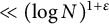 $\ll (\log N)^{1+\varepsilon }$
, for each
 $\varepsilon>0$
. Thus, the above corollary generalizes and sharpens a result of Weiß and Skill [Reference Weiß and Skill28], stating that
 $(\phi n)_{n=1}^\infty $
has Poissonian pair correlations on each scale
 $\beta < 1$
, where
 $\phi $
denotes the Golden ratio
 $\frac {\sqrt {5}+1}{2}$
. Furthermore, the condition on
 $A_N$
is known to be true for algebraic
 $\alpha $
, due to Roth’s famous approximation theorem.
Finally, we remark that, if one so wished, one could readily replace the
 $N^{\varepsilon }$
-terms in Corollary B.2 by appropriate powers of logarithms.
Appendix C The Rudnick–Sarnak obstruction
In this final appendix, we detail an obstruction to studying the higher-order correlation function
 $R_k(\alpha ,L,N,g)$
. This obstruction is a generalization of a fundamental observation of Rudnick and Sarnak [Reference Rudnick and Sarnak23, Section 4], which those authors made in the context of constant L and for the triple correlation function of
 $(\alpha n^2 \, \text {mod } 1)_{n=1}^\infty $
. We address the more general situation of sequences of the shape
 $(\alpha n^d \, \text {mod } 1)_{n=1}^\infty $
, where
 $d\geqslant 2$
is a fixed integer. We are also interested in identifying the full range of L in which the obstruction persists.
To this end, for a compactly supported smooth test function
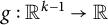 $g:\mathbb {R}^{k-1} \rightarrow \mathbb {R}$
, we define the correlation function
 $R_{k}^{d}(\alpha ,L,N, g)$
by
 $$ \begin{align*}R_{k}^{d}(\alpha,L,N, g): = \frac{1}{N}\sum\limits_{\substack{1 \leqslant x_1, \dots, x_k \leqslant N \\ \text{distinct}}} g\left(\frac{N}{L} \{ \alpha (x_1^d - x_2^d)\}_{\mathrm{sgn}}, \dots, \frac{N}{L} \{ \alpha (x_{k-1}^d - x_k^d)\}_{\mathrm{sgn}}\right),\end{align*} $$
where
 $$ \begin{align*} \{ \cdot \}_{\mathrm{sgn}}:\mathbb{R} \longrightarrow (-1/2,1/2]\end{align*} $$
denotes the signed distance to the nearest integer. Rudnick and Sarnak’s approach to pair correlations, like in Appendix A, involves showing that
 $$ \begin{align*} \int\limits_0^1 \left(R_2^d(\alpha,L,N,g) - L \frac{N-1}{N}\widehat{g}(0)\right)^2 \, d\alpha = o_g(L^2),\end{align*} $$
as
 $N \rightarrow \infty $
. Therefore, in order to make a similar approach work for the higher k-point correlation functions, one would need
 $$ \begin{align} \int\limits_{0}^{1} \left( R_k^d(\alpha,L,N,g) - L^{k-1} \frac{(N)_{k}}{N^k}\widehat{g}(\mathbf{0}) \right)^2 \, d\alpha = o_{d,k,g}(L^{2(k-1)}), \end{align} $$
as
 $N \rightarrow \infty $
, where
 $\mathbf {0}$
is the zero vector in
 $\mathbb {R}^{k-1}$
and
 $(N)_{k}=N(N-1)\ldots (N-k+1)$
abbreviates the kth falling factorial. Our purpose here is to show that, for certain ranges of d, k, and L, equation (C.1) cannot hold.
Indeed, by applying the Poisson summation formula, one may expand
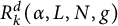 $ R_k^d(\alpha ,L,N,g) $
into a Fourier series
 $$ \begin{align*} R_k^d(\alpha,L,N,g) = \sum\limits_{\ell \in \mathbb{Z}} c_{k,\ell}^d(L,N,g) e(\ell \alpha),\end{align*} $$
with certain Fourier coefficients
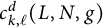 $c_{k,\ell }^d(L,N,g)$
. One may compute
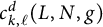 $c_{k,\ell }^d(L,N,g)$
explicitly. For a given vector
 $\mathbf {a}\in \mathbb {Z}^{k-1}$
, let
 $S_{\mathbf {a},k,\ell }^d(N)$
denote the set of integer vectors
 $\mathbf {x}\in \mathbb {N}^{k}$
, with distinct components
 $1\leqslant x_i \leqslant N$
, satisfying the Diophantine equation
 $$ \begin{align*}a_1 (x_1^d - x_2^d)+\cdots + a_{k-1}(x_{k-1}^d-x_k^d)=\ell. \end{align*} $$
One readily verifies that
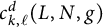 $ c_{k,\ell }^d(L,N,g)$
is of the special form
 $$ \begin{align} c_{k,\ell}^d(L,N,g) = \frac{L^{k-1}}{N^{k}}\sum_{\mathbf{a} \in \mathbb{Z}^{k-1}} \vert S_{\mathbf{a},k,\ell}^d(N) \vert \,\, \widehat{g}\left(\frac{L}{N} \mathbf{a}\right). \end{align} $$
From Parseval, we conclude that
 $$ \begin{align*}\int_0^1\left( R_k^d(\alpha,L,N,g) - L^{k-1} \frac{(N)_{k}}{N^k}\widehat{g}(\mathbf{0}) \right)^2 \, d\alpha = \sum\limits_{ \ell \neq 0} \vert c_{k, \ell}^d(L,N,g)\vert^2.\end{align*} $$
Now, let
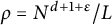 $\rho = N^{d+1 + \varepsilon }/L$
. We observe that if
 $\vert \ell \vert \geqslant \rho $
and
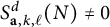 $S_{\mathbf {a},k,\ell }^d(N) \neq 0$
, then
 $\Vert \mathbf {a}\Vert _\infty \geqslant N^{1+\varepsilon }/L(k-1)$
. Therefore, from the rapid decay of
 $\widehat {g}$
and the formula (C.2), we conclude that
 $\vert c_{k,\ell }^d(L,N,g) \vert = O_{\varepsilon ,g,k,K}(N^{-K})$
for such
 $\ell $
. Hence,
 $$ \begin{align*}\sum\limits_{\ell \neq 0} \vert c_{k,\ell}^d(L,N,g)\vert ^2 = \sum\limits_{0 < \vert \ell\vert \leqslant \rho} \vert c_{k,\ell}^d(L,N,g)\vert^2 + O_{\varepsilon,g,k,K}(N^{-K}).\end{align*} $$
To estimate the right-hand side, we note that, by the Cauchy–Schwarz inequality,
 $$ \begin{align*}\rho \sum\limits_{ 0 < \vert \ell \vert \leqslant \rho} \vert c_{k,\ell}^d(L,N,g)\vert^2 \geqslant \bigg\vert \sum_{ 0< \vert \ell \vert \leqslant \rho} c_{k,\ell}^d(L,N,g) \bigg\vert^2. \end{align*} $$
The sum inside the absolute value on the right-hand side equals, up to a term of size
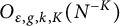 $O_{\varepsilon ,g,k,K}(N^{-K})$
, the quantity
 $$ \begin{align*} \sum\limits_{ \ell \in \mathbb{Z}} c_{k,\ell}^d(L,N,g) e(0) - L^{k-1} \frac{(N)_{k}}{N^k}\widehat{g}(\mathbf{0}),\end{align*} $$
which is
 $$ \begin{align*}R_k^d(0,L,N,g) + O_{g}(L^{k-1}).\end{align*} $$
Assuming that
 $g(\mathbf {0}) \neq 0$
and
 $L/N = o(1)$
as
 $N\rightarrow \infty $
, this is equal to
 $$ \begin{align*}N^{k-1}(1+o(1))g(\mathbf{0}),\end{align*} $$
as
 $N\rightarrow \infty $
. Now, by combining these considerations, we conclude that
 $$ \begin{align*} &\int\limits_{0}^{1} \left(R_k^d(\alpha,L,N,g) - L^{k-1} \frac{(N)_k}{N^k} \widehat{g}(\mathbf{0})\right)^2 \, d\alpha \\&\qquad \gg_{\varepsilon,g,k} \frac{1}{\rho} N^{2(k-1)} \vert g(\mathbf{0})\vert^2 = L N^{2k - d-3 - \varepsilon} \vert g(\mathbf{0})\vert^2. \end{align*} $$
If (C.1) is to hold for all functions g, for each
 $\varepsilon> 0$
, we must have
 $$ \begin{align*}L\gg_{g,\varepsilon,k} N^{\frac{2k-d-3-\varepsilon}{2k-3}} = N^{1 - \frac{d+\varepsilon}{2k-3}}. \end{align*} $$
In particular, for
 $k=3$
and
 $d=2$
, the convergence (C.1) fails unless
 $L\gg N^{\frac {6-5-\varepsilon }{6-3}}= N^{\frac {1-\varepsilon }{3}}$
. This justifies the statements we made in the introduction to the effect that the Rudnick–Sarnak obstruction for triple correlations extends throughout the range
 $L<N^{1/3}$
.
We also note, however, that as soon as
 $$ \begin{align*} d> 2k-3,\end{align*} $$
there is no such obstruction (for L constant in terms of N).
The failure of (C.1) is an artefact of the integrand having a large spike when
 $\alpha \approx 0$
(and more generally, the integrand has large spikes when
 $\alpha $
is very well approximated by rationals with small denominators). One wonders whether
 $L^2$
-convergence (C.1) can be recovered by restricting to the “minor arcs,” but this also appears to be a difficult problem.
Acknowledgment
We would like to thank Zeev Rudnick and Christoph Aistleitner for helpful comments relating to previous versions of the manuscript, and Andrew Granville and Dimitris Koukoulopoulos for many interesting conversations. We would also like to thank several anonymous referees for their suggestions and corrections.



