1. Introduction
Understanding the flow around the bluff body has been an active area of study in fluid mechanics. Due to the typical vortex shedding characteristics and the wide range of applications, such as the landing gear of aircraft, the stay cables of bridges, the pantographs of high-speed trains, and marine pipelines, investigations of flow around a circular cylinder have received wide attention for many decades (Jiang et al. Reference Jiang, Cheng, Draper, An and Tong2016; Kim, Park & Choi Reference Kim, Park and Choi2024; Maryami, Arcondoulis & Liu Reference Maryami, Arcondoulis and Liu2024). The previous studies show that the flow separation and the wake vortex shedding occur when the Reynolds number is over a critical value (Williamson Reference Williamson1996; Jiang & Cheng Reference Jiang and Cheng2017). The alternate vortex shedding brings unsteady dynamic loads, resulting in structural vibrations and acoustic noises (Octavianty & Asai Reference Octavianty and Asai2016; Duan & Wang Reference Duan and Wang2021). Therefore, effective control of vortex shedding is essential in engineering applications, and the related control methods mainly include passive and active techniques (Choi, Jeon & Kim Reference Choi, Jeon and Kim2008; Feng & Wang Reference Feng and Wang2010; Cicolin et al. Reference Cicolin, Buxton, Assi and Bearman2021; Wu, Wang & Zhou Reference Wu, Wang and Zhou2022; Silva & Assi Reference Silva and Assi2024). A rigid splitter plate installed at the rear of a cylinder is an efficient passive strategy to change interaction of the cylinder shear layers, which further controls the wake shedding pattern and reduces the drag (Assi, Bearmana & Kitney Reference Assi, Bearman and Kitney2009; Chauhan et al. Reference Chauhan, Dutta, More and Gandhi2018; Duan & Wang Reference Duan and Wang2021; Sharma & Dutta Reference Sharma and Dutta2021; Sun et al. Reference Sun, Wang, Hu, Lin and Fan2022; Wang & Li Reference Wang and Li2023; Zhou et al. Reference Zhou, Qiu, Li, Wang, Zhou and Liu2024).
The flow behaviour around an isolated circular cylinder with a splitter plate is influenced by the Reynolds number Re and
 $L/D$
, where L represents the splitter plate length, and D is the cylinder diameter, and
 $L/D$
has a significant influence for modifying vortex shedding and wake dynamics of the cylinder. When the splitter plate is installed at the rear of the cylinder, it suppresses interaction of the cylinder shear layers, which facilitates the shear layers to elongate downstream before forming the wake vortices (Anderson & Szewczyk Reference Anderson and Szewczyk1997; Ali, Doolan & Wheatley Reference Ali, Doolan and Wheatley2011; Liu, Deng & Mei Reference Liu, Deng and Mei2016; Chauhan et al. Reference Chauhan, Dutta, More and Gandhi2018; Duan & Wang Reference Duan and Wang2021). The early experiments of Gerrard (Reference Gerrard1966) at Re = 20 000 showed that the Strouhal number St was decreased from 0.2 to 0.18 as
 $L/D$
increased from 0 to 1, and St was expressed as
 $ St=fD/U_\infty$
, where
 $f$
denoted the vortex shedding frequency, and
 $U_\infty$
denoted the incoming velocity. Apelt, West & Szewczyk (Reference Apelt, West and Szewczyk1973) observed experimentally that
 $St$
increased
 $ 10\,\%$
at
 $L/D=0.25$
for
 $ 10\,000\lt {Re}\lt 50\,000$
, and
 $St$
gradually decreased with increasing
 $L/D$
for
 $0.25\leqslant L/D \leqslant 1$
. Compared to
 $L/D=0$
, the mean drag coefficient
 $C_d$
decreased by nearly 31 % at
 $L/D=1$
, and the minimum values of
 $St$
and
 $C_d$
were found at
 $L/D=1$
. The authors also pointed out that the flow characteristics were changed strongly by the short splitter plate for
 $L/D \leqslant 1$
. The experiments of Akilli et al. (Reference Akilli, Karakus, Akar, Sahin and Tumen2008) at
 $Re=6300$
suggested that
 $St$
was decreased when
 $L/D$
was increased for
 $0 \leqslant L/D \leqslant 0.6$
. In addition, some studies indicate that the elongation of the cylinder shear layers facilitates the decrease of
 $St$
when the splitter plate is short (approximately
 $L/D \leqslant 1$
) (Ali et al. Reference Ali, Doolan and Wheatley2011; Liu et al. Reference Liu, Deng and Mei2016). When the splitter plate is long (approximately
 $L/D \gt 1$
), the variations of
 $St$
are associated with the interaction of the long splitter plate and wake vortex (Kwon & Choi Reference Kwon and Choi1996; Chauhan et al. Reference Chauhan, Dutta, More and Gandhi2018; Zhou et al. Reference Zhou, Qiu, Li, Wang, Zhou and Liu2024).
The fluid–structure interaction of the wake vortex and splitter plate has been explored by previous works. The shedding wake vortices interact with the downstream splitter plate, which facilitates the roll-up and separation of the wall shear layer of the splitter plate, which leads to generation of the secondary vortex on the trailing edge of the splitter plate (Kwon & Choi Reference Kwon and Choi1996; Ali et al. Reference Ali, Doolan and Wheatley2011; Liu et al. Reference Liu, Deng and Mei2016, Reference Liu, Li, Li, Zhou and Qiu2024b
; Chauhan et al. Reference Chauhan, Dutta, More and Gandhi2018; Duan & Wang Reference Duan and Wang2021; Sharma & Dutta Reference Sharma and Dutta2021). In an experimental study of Chauhan et al. (Reference Chauhan, Dutta, More and Gandhi2018), they investigated the flow of an isolated square cylinder at
 $Re=485$
, and thought that the increase of
 $St$
for
 $2 \lt L/D \leqslant 3$
was a result of the interaction of the cylinder shear layers and the secondary vortex. Duan & Wang (Reference Duan and Wang2021) found that the fluctuation with a high frequency was increased at
 $L/D=2$
, which was caused by the interaction of the wake vortex and secondary vortex, which also led to high frequency noise. In a recent investigation of Zhou et al. (Reference Zhou, Qiu, Li, Wang, Zhou and Liu2024) for
 $Re=3900$
, they observed experimentally movement of the secondary vortex for
 $0.25 \leqslant L/D \leqslant 1$
; additionally, the longer splitter plate also provided disturbances that facilitated destabilisation of the wake vortex for
 $L/D \geqslant 1$
, thus the wake vortex was easily dissipated. Moreover, it is reported that the velocity fluctuations in the wake region are reduced with increasing
 $L/D$
, which is due to the splitter plate suppression on the wake vortices (Akilli et al. Reference Akilli, Karakus, Akar, Sahin and Tumen2008; Cui, Feng & Hu Reference Cui, Feng and Hu2022; Zhou et al. Reference Zhou, Qiu, Li, Wang, Zhou and Liu2024).
As mentioned above, the previous studies pay more attention to the influences of the splitter plate on the flow around the isolated circular cylinder placed in uniform incoming flow. In practice, the cylindrical structure is often placed near a wall in some engineering applications, such as the seabed oil pipeline and the heat exchanger tube adjacent to a wall (Jiang et al. Reference Jiang, Cheng, Draper and An2017; Liu et al. Reference Liu, Qi, Zhou, Li, Tao and Qiu2023). When the circular cylinder is placed in proximity to the wall, the interaction of the wall boundary layer flow and near-wall cylinder wake causes complex wake dynamics (Jiang & Cheng Reference Jiang and Cheng2017; Zhang et al. Reference Zhang, Xia, Qiu, Dong and Liu2023, Reference Zhang, Ma, Xia, Qiu and Liu2024), which affects the vortex-induced vibration of the near-wall cylindrical structure (Hsieh, Low & Chiew Reference Hsieh, Low and Chiew2016; Liu & Gao Reference Liu and Gao2022; Li et al. Reference Li, Li, Wu, Chong, Wang, Zhou and Liu2023). Therefore, comprehensive study of the splitter plate influences on the vortex shedding and wake dynamics of the cylinder in proximity to the wall is helpful for exploring optimal flow-control strategy in reducing vibration of the near-wall cylindrical structure in complex turbulent flow.
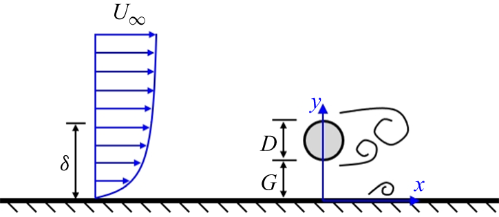
In figure 1, the flow behaviour of a near-wall cylinder is influenced by the incoming flow condition (laminar boundary layer or turbulent boundary layer),
 $Re$
, the relative boundary layer thickness
 $\delta /D$
, and gap ratio
 $G/D$
, where
 $G$
is the gap size. The flow characteristics are affected significantly by
 $G/D$
. When the cylinder is gradually close to the wall, the gap flow beneath the cylinder deflects away from the wall, resulting in the asymmetrical cylinder wake (Sarkar & Sarkar Reference Sarkar and Sarkar2010; He et al. Reference He, Wang, Pan, Feng, Gao and Rinoshika2017; Ouro, Muhawenimana & Wilson Reference Ouro, Muhawenimana and Wilson2019). Moreover, the influences of
 $G/D$
on the vortex shedding frequency are associated with
 $Re$
. Some studies suggest that
 $St$
is insensitive to larger
 $G/D$
when
 $Re$
is relatively higher (approximately
 $Re\gt 3000$
) (Bearman & Zdravkovich Reference Bearman and Zdravkovich1978; Taniguchi & Miyakoshi Reference Taniguchi and Miyakoshi1990; Lei, Cheng & Kavanagh Reference Lei, Cheng and Kavanagh1999; Price et al. Reference Price, Sumner, Smith, Leong and Paidoussis2002; Wang & Tan Reference Wang and Tan2008; Ouro et al. Reference Ouro, Muhawenimana and Wilson2019). In addition, previous studies report the
 $G/D$
influences on
 $St$
in lower Reynolds number flow (approximately
 $Re\lt 2000$
), and it is found that
 $St$
is sensitive to
 $G/D$
,
 $St$
presents an obvious increase when
 $G/D$
is decreased to the critical gap ratio
 $(G/D)_{cr}$
(where
 $(G/D)_{cr}$
is approximatively 0.2–0.5), and
 $St$
is finally decreased with further decrease of
 $G/D$
due to the wall suppression on the alternate wake vortices (Price et al. Reference Price, Sumner, Smith, Leong and Paidoussis2002; Sarkar & Sarkar Reference Sarkar and Sarkar2010; He et al. Reference He, Wang, Pan, Feng, Gao and Rinoshika2017; Zhou et al. Reference Zhou, Qiu, Li and Liu2021; Li et al. Reference Li, Wang, Qiu, Wu, Zhou, Fu and Liu2022a
,
Reference Li, Wang, Qiu, Wu, Zhou, Fu and Liub
; Jiang et al. Reference Jiang, Ju, Guo and Wang2024).
Sketch of flow around a circular flow in proximity to a wall, based on vortical structure in He et al. (Reference He, Wang, Pan, Feng, Gao and Rinoshika2017) and Zhou et al. (Reference Zhou, Qiu, Li and Liu2022).

The evolution characteristics of the vortical structures of the near-wall cylinder have been reported by previous works. The shedding wake vortices interact with the wall boundary layer, which brings complex vortex interaction. When the wake vortices are moved downstream, the wake vortices provide disturbance for the wall boundary layer, which causes an adverse pressure gradient on the wall; the wall boundary layer becomes unstable and is separated, and the secondary vortex is generated from the separated boundary layer (Doligalski, Smith & Walker Reference Doligalski, Smith and Walker1994; Kyriakides et al. Reference Kyriakides, Kastrinakis, Nychas and Goulas1999; Pan et al. Reference Pan, Wang, Zhang and Feng2008; He et al. Reference He, Pan, Feng, Gao and Wang2016). He, Pan & Wang (Reference He, Pan and Wang2013a
) examined the lift-up and three-dimensional destabilisation process of the secondary vortex at
 $G/D=1$
by particle image velocimetry (PIV) experiments. Similar experiments were carried out by He et al. (Reference He, Wang, Pan, Feng, Gao and Rinoshika2017) at
 $Re=1072$
, and by Zhou et al. (Reference Zhou, Qiu, Li and Liu2021) at
 $Re=1500$
, and they also examined the
 $G/D$
influences on evolution of vortical structures; it was observed that the strength of the lower wake vortex was weaker at
 $G/D=0.25$
and
 $0.5$
due to the wall suppression on the vortex formation. In addition, the secondary vortex evolved downstream with the lower wake vortex at
 $G/D=1$
. By a numerical investigation for
 $6666 \leqslant Re \leqslant 13\,333$
, Ouro et al. (Reference Ouro, Muhawenimana and Wilson2019) pointed out that the secondary vortex generation was not obvious as
 $G/D$
increased from 0.5 to 1, and it was due to the reduction of interaction between the wake vortex and the wall boundary layer at
 $G/D=1$
.
Compared with the near-wall cylinder placed in a laminar boundary layer or thin turbulent boundary layer, the complicated wake dynamics is produced when the near-wall cylinder is immersed in a turbulent boundary layer due to the interaction between the near-wall cylinder wake and the boundary layer flow that carries shear and turbulence fluctuations (Grass et al. Reference Grass, Raven, Stuart and Bray1984; Liu & Gao Reference Liu and Gao2022; Zhou et al. Reference Zhou, Qiu, Li and Liu2022). Grass et al. (Reference Grass, Raven, Stuart and Bray1984) used the hydrogen bubble visualisation to investigate flow structures of a near-wall cylinder at
 $1470 \leqslant Re \leqslant 4320$
and
 $\delta /D=6$
. Compared with the near-wall cylinder placed in the thin boundary layer, they observed that the wake structures of the cylinder at
 $G/D=0.3$
and
 $1$
were somewhat distorted by the turbulence in the thick boundary layer, and it was attributed to the effects of the velocity gradient and turbulence intensity of the incoming turbulent flow. Liu & Gao (Reference Liu and Gao2022) carried out experiments to examine vortex-induced vibration of a near-wall cylinder at
 $Re=16\,000$
and
 $\delta /D=4.1$
, and it was reported that the swirling strength of the lower wake vortex decreased dramatically as
 $G/D$
decreased from 1 to 0, compared with that of the upper wake vortex, which was affected by the velocity gradient of the boundary layer flow, which triggered effectively the transverse vibration of the cylinder. Zhou et al. (Reference Zhou, Qiu, Li and Liu2022) investigated vortex shedding of a near-wall cylinder at
 $Re=1000$
and
 $\delta /D=6.7$
, and they found that the swirling strength of the upper wake vortex was slightly bigger than that of the lower wake vortex due to velocity differences of incoming flow, that
 $St$
was increased as
 $G/D$
decreased from 1 to 0.5, and that the increase of
 $St$
was attributed to the combined effects of the gap flow and the velocity gradient.
In addition, the effects of
 $\delta /D$
on the flow characteristics of the near-wall cylinder are reported. Lei et al. (Reference Lei, Cheng and Kavanagh1999) experimentally found that
 $ C_{d}$
was increased with increasing
 $G/\delta$
when the cylinder was fully or partly immersed in a boundary layer, and the critical gap ratio was decreased as
 $\delta /D$
increased. The two-dimensional numerical study of Kazeminezhad, Bakhtiary & Shahidi (Reference Kazeminezhad, Bakhtiary and Shahidi2010) showed that
 $ C_{d}$
and mean lift coefficient
 $ C_{l}$
were slightly decreased as
 $\delta /D$
increased from 0.3 to 3. Similar results were reported by Chen et al. (Reference Chen, Wang, Sun and Wang2020), and they examined the effects of
 $\delta /D$
on the flow of a cylindrical pipeline over a fully scoured seabed;
 $ C_{d}$
and
 $St$
were decreased when
 $\delta /D$
increased from 0.5 to 3, and also, the size of the vortices downstream of the cylinder became large and their vorticities became small with increasing
 $\delta /D$
. The three-dimensional numerical study of Zhang et al. (Reference Zhang, Ji, Chen, Hua and Srinil2021) at
 $Re=350$
revealed that the strength and size of the wake vortices gradually decreased with increasing
 $\delta /D$
for a fixed
 $G/D$
, and the flow three-dimensionality was also gradually weakened.
Due to the academic value and wide range of engineering applications, some flow control methods are also applied to modify the flow around the near-wall cylinder. In an experimental investigation of He & Wang (Reference He and Wang2015) for
 $Re=1072$
, the synthetic jet at the rear stagnation point of the cylinder was used to modify the wake shedding pattern at
 $G/D=2$
, and they found that the wake shedding pattern was changed by adjusting excitation frequency of the synthetic jet. Additionally, the destabilisation process of the wall secondary vortex was promoted when the synthetic jet was introduced, which promoted transition of the downstream boundary layer. Zhang & Shi (Reference Zhang and Shi2016) examined the flow around the cylinder with splitter plate near a moving wall by a two-dimensional numerical study for
 $200 \leqslant Re \leqslant 400$
,
 $L/D=1$
and
 $0.1 \leqslant G/D \leqslant 3$
. Compared with the cylinder without a splitter plate near a moving wall,
 $C_d$
was obviously reduced when the cylinder carried the splitter plate. In a recent two-dimensional numerical investigation of Liu et al. (Reference Liu, Li, Li, Zhou and Qiu2024b
), they studied the influences of
 $L/D$
on the flow control of the near-wall cylinder for
 $Re=500$
, where
 $L/D$
ranged from 0 to 4.5, and
 $0.1 \leqslant G/D \leqslant 0.9$
. Their results showed that
 $St$
was reduced as
 $L/D$
increased from 0 to 1 at
 $G/D \geqslant 0.3$
, the wake shedding completely disappeared at
 $G/D=0.1$
, and the minimum
 $C_d$
appeared in the range
 $0.5 \leqslant L/D \leqslant 1$
when
 $G/D \geqslant 0.3$
.
In summary, the previous studies have led to a good understanding of the splitter plate influences on the wake dynamics of an isolated circular cylinder placed in uniform incoming flow. However, to the best knowledge of the authors, there remains a dearth of research exploring the splitter plate influences on flow physics of a circular cylinder placed in complex turbulent flow, and the influences of
 $L/D$
on the wake characteristics of a near-wall cylinder placed in the wall boundary layer flow have not been reported experimentally in the literature; in addition, the vortex shedding characteristics and vortex evolution for different
 $G/D$
and
 $L/D$
need to be further explored at medium Reynolds number. Motivated by the knowledge gaps, the present study will examine the influences of
 $L/D$
on the wake characteristics and vortex evolution of a near-wall cylinder immersed in the turbulent boundary layer flow by PIV experiments; the mechanism of the splitter plate suppression on the wake fluctuations is revealed, and the influences of the splitter plate on the interaction of the cylinder wake and boundary layer flow are presented. The present investigations may provide insights into the passive flow-control of the near-wall cylindrical structure placed in complex wall turbulent flow, and it will be helpful for understanding the modulation of interaction between a bluff body wake and boundary layer flow (Thompson, Leweke & Hourigan Reference Thompson, Leweke and Hourigan2021; Chalmers, Fang & Tachie Reference Chalmers, Fang and Tachie2023).
In the present PIV experiments, the Reynolds number is fixed at
 $Re=3900$
, the relative boundary layer thickness is
 $\delta /D=2.13$
, and the gap ratios are selected as
 $G/D=0.25$
, 0.5 and 1 due to the typical wake characteristics (He et al. Reference He, Wang, Pan, Feng, Gao and Rinoshika2017; Ouro et al. Reference Ouro, Muhawenimana and Wilson2019; Zhou et al. Reference Zhou, Qiu, Li and Liu2021). The short rigid splitter plate is used to modify the flow behaviour, and
 $L/D$
is selected as 0, 0.25, 0.5, 0.75 and 1. The remainder of this paper is organised as follows. The PIV experimental procedures and the data processing methods are presented in § 2, and § 3 shows the main findings and discussions. The major conclusions are summarised in § 4.
2. Experimental set-up and methodology
2.1. Experimental model
The recirculating open water channel where the PIV experiments were carried out had a test section of 6000 mm
 $\times$
300 mm
 $\times$
400 mm (length
 $\times$
width
 $\times$
height) at Shanghai Institute of Technology (Zhou et al. Reference Zhou, Qiu, Li, Wang, Zhou and Liu2024). The experimental schematic and PIV test region are shown in figure 2. The free-stream incoming velocity was
 $U_\infty =0.2$
m s−1, with turbulent intensity less than 2.5 %. In figure 2, a smooth flat plate of size 2400 mm
 $\times$
285 mm
 $\times$
15 mm (length
 $\times$
width
 $\times$
thickness) was positioned horizontally 30 mm above the bottom wall of the water channel, and the leading edge of the flat plate was tapered to reduce the influences of the flow separation from the plate leading edge on the downstream flat plate boundary layer flow. The incoming boundary layer on the flat plate was tripped with a circular rod to promote development of the boundary layer (Lei et al. Reference Lei, Cheng and Kavanagh1999; He, Wang & Rinoshika Reference He, Wang and Rinoshika2019; Zhou et al. Reference Zhou, Qiu, Li and Liu2022; Tang & Jiang Reference Tang and Jiang2024), and it is worth mentioning that the circular rod or some obstacles (trip wire, sandpaper and toothed barrier) placed downstream of the leading edge of the flat plate were efficient strategies to promote development of the boundary layer in a finite-length test section (Marusic et al. Reference Marusic, Chauhan, Kulandaivelu and Hutchins2015; Tang et al. Reference Tang, Wu, Jia and Jiang2018; Fang & Tachie Reference Fang and Tachie2019a
; Essel, Tachie & Balachandar Reference Essel, Tachie and Balachandar2021). In figure 2(a), the circular rod has diameter
 $d=8$
mm, and its spanwise length is 285 mm; it is fixed in the flat plate 300 mm downstream of the plate leading edge.
The experimental schematic: (a) sketch of the experimental arrangement; (b) side view of the test region.

The experimental circular cylinder was placed horizontally at the flat plate, 1000 mm downstream of the circular rod. It was mounted between two rectangular end-plates, which were transparent, and they were fixed on the flat plate. Each end-plate had size 200 mm
 $\times$
180 mm
 $\times$
5 mm (length
 $\times$
height
 $\times$
thickness), and its leading edge was located 40 mm upstream of the cylinder centre. The gap between the end-plate and the water channel sidewall was approximately 7.5 mm, and the leading edge of the end-plate had a chamfer of
 $45^{\circ }$
, which thereby reduced the influence of the wall interference and minimised flow distortion in the area surrounding the cylinder (Zhou et al. Reference Zhou, Qiu, Li and Liu2021; Chalmers et al. Reference Chalmers, Fang and Tachie2023). The cylinder diameter was
 $D=20$
mm, its spanwise length was 275 mm, the ratio of the spanwise length to the diameter was 13.75, and it should be noted that the ratio was considered large enough to present obvious two-dimensional flow characteristics in the central region of the near wake (Wang & Tan Reference Wang and Tan2008). The gap
 $G$
denotes the vertical distance between the lower surface of the cylinder and the flat plate, and the ratios of
 $G$
to
 $D$
were
 $G/D=0.25$
, 0.5 and 1 in current experiments. In figure 2(b), the splitter plate was installed at the rear of cylinder, and it was parallel with the flat plate. The spanwise length of the splitter plate was 275 mm, equal to that of the cylinder, and the streamwise length (width) of the splitter plate was
 $L=5$
, 10, 15 and 20 mm. In addition, experiments of flow past a near-wall cylinder without the splitter plate (
 $L=0$
mm) were conducted, thus the ratios of
 $L$
to
 $D$
were
 $L/D=0$
, 0.25, 0.5, 0.75 and 1. The splitter plate had larger thickness 2 mm (not presented in the figure), which was not deformed in the flow and could be as a rigid plate (Akilli et al. Reference Akilli, Karakus, Akar, Sahin and Tumen2008; Zhou et al. Reference Zhou, Qiu, Li, Wang, Zhou and Liu2024).
The material of the cylinder and splitter plate was polymethyl methacrylate. In order to reduce reflection of the laser on the experimental model, spray paint was used to paint black the surfaces of the cylinder and splitter plate. Additionally, a transparent gap of approximately 1 mm was left on the middle position of the splitter plate, so that the laser easily passed through the plate to illuminate the flow fields (see figure 2
a). The distance between the liquid level and the flat plate was approximatively 255 mm, and the influences of small fluctuations of the liquid level on PIV test region could be neglected. The PIV experiments were conducted in water temperature approximately 19
 $^{\circ }$
C, the kinematic viscosity of water was approximately
 $\nu =1.0315 \times 10^{-6}\ \textrm m^{2}\,\textrm{s}^{-1}$
, and the Reynolds number was calculated by
 $Re=U_\infty D/\nu$
at approximately
 $Re=3900$
. In our coordinate system, the streamwise direction, vertical direction and spanwise direction were denoted by
 $x$
,
 $y$
and
 $z$
, respectively.
2.2. The PIV measurement
The time-resolved PIV system provided by LaVision Inc. was applied to conduct experiments. The tracer particles made by the polyamide resin particle were seeded uniformly in the water channel, and the diameter and density of the tracer particles were
 ${d}_P=20$
 $\unicode {x03BC}$
m and
 $\rho _P=1030\,\mathrm{kg}\,\mathrm{m}^-{^3}$
, respectively. The Stokes number (
 $S_P$
) of the particles was used to assess the subsequent performance of the particle, calculated by
 \begin{equation} S_P=\frac {t_P}{t_f}=\frac {d_P^2(\rho _P-\rho _f)}{18\rho _f\nu t_f}, \end{equation}
where
 $t_P$
is the response time of the particles,
 $t_f$
is the characteristic temporal scale,
 $t_f=D/U_\infty$
, and
 $\rho _f$
represents the density of the water. By calculation,
 $t_P$
was
 $6.463 \times 10^{-7}$
s, and
 $t_f$
was 0.1 s, thus the Stokes number was approximatively
 $S_P=6.463 \times 10^{-6}$
, and the value of the present
 $S_P$
was less than 0.05 reported by Samimy & Lele (Reference Samimy and Lele1991), which suggested that the particles could follow faithfully the flow of fluids in current experiments.
As illustrated in figure 2(a), the PIV region was perpendicular to the flat plate and located at the middle section of the cylinder in the
 $x$
–
 $y$
plane. The particles were illuminated by a double-pulse Nd: YAG laser with laser wavelength 532 nm, and the laser thickness was approximatively 1 mm in the PIV test region. A Phantom M110 camera was applied to capture the particle images; the lens was AF Nikkor (50 mm), and the aperture was selected as
 $f/1.4$
. The resolution of the camera was 1280 pixels
 $\times$
800 pixels, and the size of the PIV field was approximatively 165 mm
 $\times$
100 mm (
 $8.25D \times 5D$
) in the
 $x$
- and
 $y$
-directions, thus the magnification was approximatively 0.129 mm pixel−1. For the current experiments, it was ensured that the average diameter of the imaged particles was approximatively 2–4 pixels, so that the peak-locking errors were reduced (Michaelis, Neal & Wieneke Reference Michaelis, Neal and Wieneke2016; Scharnowski & Kähler Reference Scharnowski and Kähler2020). In addition, according to the incoming velocity
 $U_\infty =0.2\,\textrm m\,\textrm{s}^-{^1}$
, the time delay of a pair of particle images was chosen as 2800
 $\unicode {x03BC}$
s, which provided an average shift of the particle (approximatively 4.34 pixels).
The DaVis 8.4.0 software with the multi-pass interrogation algorithm was used to analyse the particle images. The size of the initial interrogation was 64 pixels
 $\times$
64 pixels with
 $50\,\%$
overlap, and the size of the final interrogation was 32 pixels
 $\times$
32 pixels with
 $75\,\%$
overlap, providing a space domain of approximatively 4.13
 $\times$
4.13 mm
 $^2$
, and the velocity vector interval was approximatively 1 mm (
 $0.05D$
). Limited by the storage capacity of the camera, a repetition of 2000 frames could be continuously captured at a time for the camera under the current spatial resolution. The sampling frequency of PIV was chosen as 100 Hz, and the sampling time of one repetition was 20 s. In the current PIV experiments, the flat-plate boundary layer flow without the presence of the cylinder was first examined, and three repetitions were conducted to expand the sample size; the total sampling time was 60 s, and a total of 6000 velocity fields were obtained to analyse boundary layer characteristics. Second, the flow around the circular cylinder in proximity to the wall for different
 $G/D$
and
 $L/D$
was examined; two repetitions were conducted, and a total of 4000 velocity fields were obtained to analyse mean statistics. The convergence test was carried out, and it was ensured that the present sample size was sufficient for the convergence of the velocity fluctuations in the time-averaged flow fields; more details about the statistical convergence are provided in Appendix A. The uncertainties
 $\varepsilon$
of time-averaged streamwise velocity
 $U$
, Reynolds streamwise normal stress
 $\overline {u^{\prime}u^{\prime}}$
and Reynolds shear stress
 $-\overline {u^{\prime}v^{\prime}}$
were expressed as (Sciacchitano & Wieneke Reference Sciacchitano and Wieneke2016)
 \begin{equation} \varepsilon (U)=\frac {\sigma (u)}{\sqrt {N}},\quad \varepsilon (\overline {u^{\prime}u^{\prime}})=\sigma (u)\,\sigma (u)\,\sqrt {\frac {2}{N}},\quad \varepsilon (-\overline {u^{\prime}v^{\prime}})=\sigma (u)\,\sigma (v)\,\sqrt {\frac {1+r_{uv}^2}{N-1}}, \end{equation}
where
 $\sigma (u)$
and
 $\sigma (v)$
represent, respectively, the standard deviations of the instantaneous streamwise velocity and vertical velocity, and
 $N$
denotes sample number, with
 $N=4000$
in the current experiments. Here,
 $r_{uv}$
is the cross-correlation coefficient of
 $u$
and
 $v$
, selected as 0.41 based on the current interrogation window of 32 pixels
 $\times$
32 pixels with
 $75\,\%$
overlap (Sciacchitano & Wieneke Reference Sciacchitano and Wieneke2016). According to the maximum
 $\sigma (u)$
and
 $\sigma (u)\,\sigma (v)$
for each case, the uncertainties of
 $U$
,
 $\overline {u^{\prime}u^{\prime}}$
and
 $-\overline {u^{\prime}v^{\prime}}$
were not greater than
 $0.682\,\%\,U_\infty$
,
 $0.416\,\%\,U_\infty ^2$
and
 $0.35\,\%\,U_\infty ^2$
, respectively.
2.3. Characteristics of boundary layer flow
First, the parameters of the boundary layer flow at the central position of the cylinder (
 $x/D=0$
) without the presence of the cylinder are presented in table 1. The flow has boundary layer thickness approximatively
 $\delta =42.52$
mm, based on the location of the velocity profile
 $U(y)/U_\infty =0.99$
, and the ratio of
 $\delta$
to
 $D$
is approximatively
 $\delta /D=2.13$
, which suggests that the experimental circular cylinder is immersed in the boundary layer flow for
 $G/D=0.25$
,
 $0.5$
and
 $1$
. The displacement thickness is approximatively
 $\delta ^\ast =5.52$
mm, obtained by
 $\delta ^\ast =\int _{0}^{\delta }(1- ({U(y)}/{U_\infty }))\,\textrm {d}y$
, and the momentum thickness is approximatively
 $\theta =4.39$
mm, obtained by
 $\theta =\int _{0}^{\delta }({U(y)}/{U_\infty })(1- ({U(y)}/{U_\infty }))\,\textrm {d}y$
. Therefore, the shape factor is approximately
 $H=1.26$
based on
 $\delta ^\ast$
and
 $\theta$
, and the shape factor is similar to the results of the turbulent boundary layer reported by previous studies (Tomkins & Adrian Reference Tomkins and Adrian2003; Tang & Jiang Reference Tang and Jiang2024), which suggests that the developed turbulent boundary layer is formed in the PIV region. It should be noted that the current turbulent boundary layer is a boundary layer produced artificially by the circular rod (Tang et al. Reference Tang, Jiang, Lu and Zhou2024; Tang & Jiang Reference Tang and Jiang2024). In table 1, the boundary layer turnover time
 $TU_\infty /\delta$
is approximately 282, where
 $T$
is the total sampling time, and the present boundary layer turnover time is close to that in He et al. (Reference He, Wang and Rinoshika2019), ensuring that the total sample time is sufficient for converged statistics of the boundary layer parameters. The friction velocity is
 $u_\tau =0.0098$
m s−1, estimated by fitting the velocity profile onto the log law (Clauser Reference Clauser1954), the von Kármán constant is selected as
 $\kappa =0.41$
, and the constant is
 $B=5.0$
. The Reynolds number based on
 $u_\tau$
is expressed as
 $Re_\tau =u_\tau \delta /\nu$
, for
 $Re_\tau =404$
.
Summary of parameters of the boundary layer flow.

(a) The profiles of time-averaged streamwise velocity
 $U^+$
, where the black solid line denotes the log law. (b) The profiles of time-averaged Reynolds stresses and streamwise velocity
 $U/U_\infty$
, where the black dash-dotted line denotes
 $\delta /D=2.13$
, and the black dashed lines denote the height of the cylinder centre in the cases
 $G/D=0.25$
,
 $0.5$
and
 $1$
.

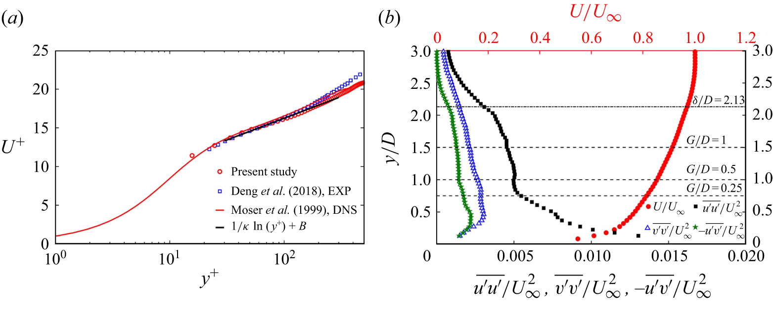
Figure 3 shows profiles of time-averaged streamwise velocity and Reynolds stresses at the central position of the cylinder without the presence of the cylinder. The profiles of streamwise velocity
 $U^+$
are presented in figure 3(a), and the experimental results at
 $Re_\tau =525$
of Deng et al. (Reference Deng, Pan, Wang and He2018) and the DNS results at
 $Re_\tau =395$
of Moser, Kim & Mansour (Reference Moser, Kim and Mansour1999) are provided for comparison. The profiles of Reynolds stresses (
 $\overline {u^{\prime}u^{\prime}}$
,
 $\overline {v^{\prime}v^{\prime}}$
,
 $-\overline {u^{\prime}v^{\prime}}$
) and streamwise velocity
 $U/U_\infty$
are shown in figure 3(b), and the height locations of the cylinder centre for the three gap ratios are presented. In figure 3(a), the vertical location
 $y^+$
is obtained by
 $y^+=yu_\tau /\nu$
, and
 $U^+$
is expressed as
 $U^+=U/u_\tau$
. The profile of
 $U^+$
agrees with that of the two works cited, and small differences in profiles of
 $U^+$
may be due to differences of
 $Re_\tau$
and research methods. The log-law region is located at approximately
 $30\lt y^+\lt 200$
; the
 $U^+$
distribution of approximately
 $y^+\lt 15$
is not precise because of the laser reflection on wall, thus it is not presented in the figure. In figure 3(b), the distributions of Reynolds stresses agree with the results investigated in previous wall turbulent boundary layer studies at comparable
 $Re_\tau$
(Tang et al. Reference Tang, Wu, Jia and Jiang2018; Essel et al. Reference Essel, Tachie and Balachandar2021; Chalmers et al. Reference Chalmers, Fang, Addai and Tachie2022). The
 $U/U_\infty$
distribution presents an obvious velocity gradient, reflecting the shear characteristics of the turbulent boundary layer flow.
Following previous studies (Fang & Tachie Reference Fang and Tachie2019b
, Reference Fang and Tachie2020; Essel et al. Reference Essel, Tachie and Balachandar2021; Chalmers et al. Reference Chalmers, Fang and Tachie2023; Essel, Balachandar & Tachie Reference Essel, Balachandar and Tachie2023; Ouedraogo & Essel Reference Ouedraogo and Essel2023; Liu et al. Reference Liu, Wang, Zhou, Li and Qiu2024c
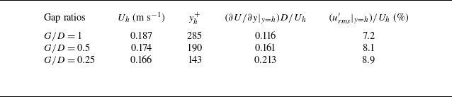
), the boundary layer parameters measured at the height of the cylinder centre could be used to assess approach flow conditions before the near-wall cylinder. Table 2 shows the relevant boundary layer parameters measured at the height of the cylinder centre for the three gap ratios. The height of the cylinder centre in wall units
 $y_h^+$
is expressed as
 $y_h^+=hu_\tau /\nu$
, where
 $h$
is the distance between the cylinder centre and the wall. Figure 3(a) shows that the height of the cylinder centre in cases
 $G/D=0.25$
and
 $0.5$
are within the log-law region, while the case
 $G/D=1$
extends into the boundary layer wake region. The mean streamwise velocity at the height of the cylinder centre,
 $U_h$
, ranges from 0.166 to 0.187 m s–1. As
 $G/D$
decreases from 1 to 0.25, the dimensionless mean shear
 $(\partial U/ \partial y\vert _{y=h})D/U_h$
and streamwise turbulence intensity
 $(u_{\it{rms}}^{\prime}\vert _{y=h})/U_h$
are increased. The thick boundary layer flow carrying the shear and turbulent fluctuations may affect wake dynamics of the near-wall cylinder at the three gap ratios.
Summary of relevant boundary layer parameters measured at the height of the cylinder centre for the three gap ratios, where the subscript
 $h$
denotes measurement at the height of the cylinder centre.

2.4. Data processing methods
2.4.1. Proper orthogonal decomposition
Proper orthogonal decomposition (POD) is an effective statistical method to extract the dominant features from flow fields (Sirovich Reference Sirovich1987; Berkooz, Holmes & Lumley Reference Berkooz, Holmes and Lumley1993; Feng, Wang & Pan Reference Feng, Wang and Pan2011; Essel et al. Reference Essel, Balachandar and Tachie2023); moreover, it is also a powerful tool to capture phase information of periodic vortex shedding (Oudheusden et al. Reference Oudheusden, Scarano, Hinsberg and Watt2005; Pan, Wang & Wang Reference Pan, Wang and Wang2013; Qu et al. Reference Qu, Wang, Feng and He2019; Li et al. Reference Li, He, Wang and Liu2021; Zhou et al. Reference Zhou, Qiu, Li and Liu2022). The snapshot POD method is used in the present study (Sirovich Reference Sirovich1987) to capture the phase of the vortex shedding and further investigate evolution process of the vortical structures. In POD analysis, the velocity fluctuations
 $\boldsymbol{u}^{\prime}(u^{\prime},v^{\prime})$
can be decomposed into the linear sum of the time coefficient
 $a_n$
and POD modes
 $\boldsymbol{\it \Phi }_n$
, which is expressed as
 \begin{equation} \boldsymbol{u}^{\prime}=\sum \limits _{n=1}^{N}a_n\boldsymbol{\it \Phi }_n, \end{equation}
where
 $N$
denotes the snapshot number. All velocity fluctuations
 $\boldsymbol{u}^{\prime}(u^{\prime},v^{\prime})$
constitute a matrix:
 $\boldsymbol{M}=[\boldsymbol{u}_1^{\prime} \boldsymbol{u}_2^{\prime} \cdots \boldsymbol{u}_N^{\prime}]$
. The autocovariance matrix is expressed as
 $\boldsymbol{C}=\boldsymbol{M}^{\textrm{T}}\boldsymbol{M}$
, thus the eigenvalues
 $\lambda _i$
and corresponding eigenvectors
 $\boldsymbol{A}_i$
can be obtained from
 $\boldsymbol{C}\boldsymbol{A}_i=\lambda _i\boldsymbol{A}_i$
.
2.4.2. Finite-time Lyapunov exponents
The finite-time Lyapunov exponents (FTLE) method can effectively identify the structure boundary, with the ridges representing the Lagrangian coherent structures (Shadden, Dabiri & Marsden Reference Shadden, Dabiri and Marsden2006; He et al. Reference He, Pan, Feng, Gao and Wang2016; Qu et al. Reference Qu, Wang, Feng and He2019; Li et al. Reference Li, Wang, Qiu, Zhou, Fu and Liu2024b
). The calculation of FTLE is based on the fluid particle trajectories that are obtained from the velocity fields, and the flow map is defined as
 $\ \Phi _{t_0}^{t_0+t_1}: \boldsymbol{x}(t_0)\rightarrow \boldsymbol{x}(t_0+t_1)$
, which maps fluid particles from the initial location at time
 $t_0$
to the location at time
 $t_0+t_1$
. The FTLE at
 $t_0$
can be calculated by
 \begin{equation} \textrm {FTLE}(\boldsymbol{x},t_0,t_1)=\frac {\textrm 1}{\lvert t_1 \rvert }\ln \left ( \lambda _{max} \left\{ \left [ \frac {\partial \boldsymbol{x}(t_0+t_1)}{\partial \boldsymbol{x}(t_0)} \right ]^{\textrm{T}} \left [\frac {\partial \boldsymbol{x}(t_0+t_1)}{\partial \boldsymbol{x}(t_0)} \right ] \right \} \right )\!, \end{equation}
where
 $\textrm {FTLE}(\boldsymbol{x},t_0,t_1)$
represents the exponential growth rate of nearby trajectories during a time interval
 $t_1$
, and
 $\lambda _{max}$
is the maximum eigenvalue of the Cauchy–Green strain tensor. In the current study, the FTLE fields are investigated for
 $G/D=1$
. The backward integration (
 $t_1\lt 0$
) is applied, a period of one vortex shedding cycle for
 $G/D=1$
and
 $L/D=0$
is selected as the integration time, and more details of the flow structures are obtained.
3. Results and discussion
3.1. The mean flow characteristics
In this subsection, the influences of
 $L/D$
on the mean flow characteristics for the three gap ratios are examined, which mainly include the time-averaged velocity, the characteristics of recirculation region and the time-averaged spanwise vorticity.
The time-averaged streamwise velocity
 $U/U_\infty$
and streamlines for nine typical cases are shown in figure 4. There is reverse flow of fluids (
 $U\lt 0$
) in the wake region; the recirculation region appears, and it is associated with shedding of the wake vortices. For
 $G/D=0.5$
and
 $1$
, the reverse flow of fluids is enhanced by the splitter plate, and the range of the recirculation region is increased when
 $L/D$
is increased. The observation is consistent with the previous studies that investigate the flow past an isolated circular cylinder (Kwon & Choi Reference Kwon and Choi1996; Akilli et al. Reference Akilli, Karakus, Akar, Sahin and Tumen2008; Tang et al. Reference Tang, Zhu, Wang, Alam, Song and Chen2022; Zhou et al. Reference Zhou, Qiu, Li, Wang, Zhou and Liu2024). For
 $G/D=0.25$
in figure 4(a–c), the variation in the range of recirculation region with
 $L/D$
is small, which is associated with the wall suppression on the wake vortices. At this gap ratio, the gap flow beneath the cylinder becomes weaker, and fewer fluids are carried into the wake region by the gap flow, which suppresses formation of the lower wake vortex of cylinder (He et al. Reference He, Wang, Pan, Feng, Gao and Rinoshika2017; Zhou et al. Reference Zhou, Qiu, Li and Liu2021), which also affects the range of the recirculation region. Therefore, the
 $L/D$
influences on the range of recirculation region are weaker for
 $G/D=0.25$
. In figure 4, the strength of the gap flow is assessed roughly by the contour line of
 $U/U_\infty =1$
below the cylinder, and the streamwise length of the contour line of
 $U/U_\infty =1$
is obviously increased when
 $L/D$
is increased for
 $G/D=0.5$
and
 $1$
, which may indicate that the gap flow strength is increased for larger
 $L/D$
. Due to the weaker gap flow for
 $G/D=0.25$
, the influences of
 $L/D$
on the strength of the gap flow are weaker, and the variation in contour line of
 $U/U_\infty =1$
below the cylinder with
 $L/D$
is small.
Time-averaged streamwise velocity
 $U/U_\infty$
for nine typical cases, superimposed on corresponding streamlines: (a–c)
 $G/D=0.25$
, (d–f)
 $G/D=0.5$
, and (g–i)
 $G/D=1$
. The red dashed lines represent contour lines of
 $U/U_\infty =0$
, and the blue dashed lines represent contour lines of
 $U/U_\infty =1$
.

The time-averaged wall-normal velocity
 $V/U_\infty$
for nine typical cases are shown in figure 5, and the peak values of
 $V/U_\infty$
in the upper and lower wake regions are presented in the figure. The peak values of
 $V/U_\infty$
can reflect magnitudes of
 $V/U_\infty$
. In the upper and lower wake regions, there are concentrated wall-normal velocities with opposite signs, which is associated with the wake vortex formation. For
 $G/D=0.5$
and
 $1$
, the peak values of
 $V/U_\infty$
are decreased when
 $L/D$
is increased. Previous works show that the splitter plate can reduce the coherence of the wake vortices of the isolated cylinder, which reduces velocity fluctuations in the wake region (Akilli et al. Reference Akilli, Karakus, Akar, Sahin and Tumen2008; Duan & Wang Reference Duan and Wang2021; Wang & Li Reference Wang and Li2023; Zhou et al. Reference Zhou, Qiu, Li, Wang, Zhou and Liu2024). For the present study, the velocity fluctuations in the wake region are also reduced by the splitter plate, which leads to weaker magnitudes of
 $V/U_\infty$
for larger
 $L/D$
. The
 $L/D$
influences on the velocity fluctuations will be discussed in § 3.4. For
 $G/D=0.25$
in figure 5(a–c), the variations of the peak values of
 $V/U_\infty$
with
 $L/D$
are small. Additionally, the magnitudes of
 $V/U_\infty$
for
 $G/D=0.25$
are less than those for
 $G/D=0.5$
and
 $1$
, which is associated with the wall suppression on the wake vortices at small gap ratio.
Time-averaged wall-normal velocity
 $V/U_\infty$
for nine typical cases: (a–c)
 $G/D=0.25$
, (d–f)
 $G/D=0.5$
, and (g–i)
 $G/D=1$
. The peak values of
 $V/U_\infty$
in the upper and lower wake regions are presented, and the red dashed lines represent contour lines of
 $U/U_\infty =0$
.

To better explain the influences of
 $L/D$
on wake development of the near-wall cylinder, the time-averaged velocity profiles
 $U/U_\infty$
at different streamwise locations are shown in figure 6. At
 $x/D=1$
and
 $1.5$
, it should be noted that the velocity distribution on the splitter plate is not shown. The obvious velocity deficit appears at
 $x/D=1$
for each
 $G/D$
, caused by blockage effects of the near-wall cylinder; moreover, the velocity deficit is decreased with the increase of
 $x/D$
. For different
 $L/D$
, the distributions of the velocity profiles are similar at
 $x/D=6$
, and the observation suggests that the
 $L/D$
influences on the mean velocity distributions are reduced in the far wake region. In figures 6(b) and 6(c), it is clear that
 $L/D$
has significant influences on distribution of the velocity deficit for
 $G/D=0.5$
and
 $1$
; the velocity deficit in the wake is enhanced by the splitter plate, and it is increased when
 $L/D$
is increased from 0 to 1, which is associated with the increase of the range of the recirculation region in figure 4. This finding is also in accordance with the results of the flow around the isolated cylinder for
 $0\lt L/D \leqslant 1$
(Zhou et al. Reference Zhou, Qiu, Li, Wang, Zhou and Liu2024). When
 $G/D$
is decreased to 0.25 in figure 6(a), the
 $L/D$
influences on distributions of the velocity profiles are weaker at different streamwise locations; in addition, the variation of the velocity deficit with
 $L/D$
is small, which also agrees with the results of figures 4 and 5. In figure 6, there is a sharp velocity jump below the cylinder, which reflects acceleration of the gap flow, which is also reported in previous works (Wang & Tan Reference Wang and Tan2008; Lin et al. Reference Lin, Lin, Hsieh and Dey2009; Zhou et al. Reference Zhou, Qiu, Li and Liu2022). For
 $G/D=0.5$
and
 $1$
, it is interesting to note that the velocity jump is increased when
 $L/D$
is increased, which reflects enhancement of the gap flow, which also confirms conclusions of figure 4. However, for
 $G/D=0.25$
, the
 $L/D$
influences on the velocity jump are small, which is due to the weaker gap flow.
Time-averaged velocity profiles
 $U/U_\infty$
at different streamwise locations. The selected streamwise locations are
 $x/D=1$
, 1.5, 2, 3, 4 and 6, for (a)
 $G/D=0.25$
, (b)
 $G/D=0.5$
, and (c)
 $G/D=1$
. The black dashed lines denote
 $U/U_\infty =0$
.

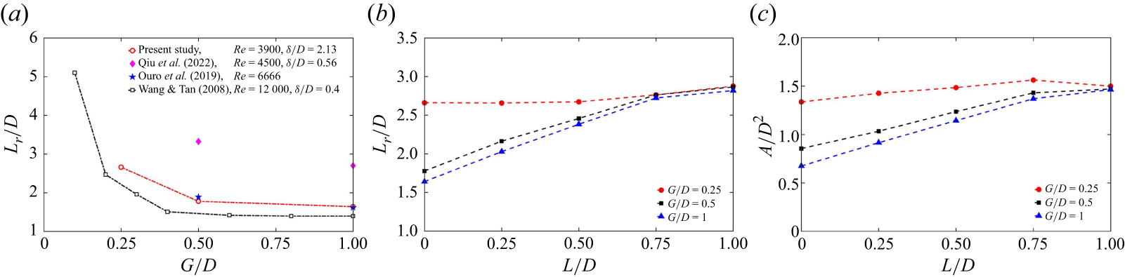
To further investigate statistic characteristics of the recirculation region behind the cylinder, the variations of the streamwise length of recirculation region (
 $L_r/D$
) and the mean recirculation area (
 $A/D^2$
) are presented in figure 7. According to the contour line
 $U/U_\infty =0$
in figure 4, the location of the saddle point is obtained, and the streamwise distance between the saddle point and the cylinder centre can be defined as the streamwise length of the recirculation region (
 $L_r$
) (Akilli et al. Reference Akilli, Karakus, Akar, Sahin and Tumen2008; Liu et al. Reference Liu, Deng and Mei2016; Duan & Wang Reference Duan and Wang2021). Following previous studies (Pearson, Goulart & Ganapathisubramani Reference Pearson, Goulart and Ganapathisubramani2013; Essel et al. Reference Essel, Tachie and Balachandar2021; Liu et al. Reference Liu, Wang, Zhou, Li and Qiu2024c
), the area of instantaneous recirculation region
 $A(t)$
is calculated in a selected range (
 $R$
), which is expressed as
 \begin{align} A(t) &=\int _{R}\xi (u(x,y,t))\,\textrm {d} x\,\textrm {d} y, \end{align}
 \begin{align} \xi (u) &= \left \{ \begin{array}{ll} 0, & u \geqslant 0, \\ 1, & u \lt 0 , \end{array} \right . \end{align}
where
 $u$
represents instantaneous streamwise velocity, and
 $\xi (u)$
is a criterion. The chosen range
 $R$
is located at
 $0.5\leqslant x/D \leqslant 6$
and
 $0\lt y/D \leqslant 3$
, and the mean recirculation area
 $A$
is obtained by (3.1).
(a) Variations of the streamwise length of the recirculation region with
 $G/D$
for
 $L/D=0$
. (b) Variations of the streamwise length of the recirculation region with
 $L/D$
. (c) Variations of the mean recirculation area with
 $L/D$
.

First, the variations of
 $L_r/D$
with
 $G/D$
for
 $L/D=0$
are presented in figure 7(a), and the results of the previous studies are also provided for comparison (Wang & Tan Reference Wang and Tan2008; Ouro et al. Reference Ouro, Muhawenimana and Wilson2019; Qiu et al. Reference Qiu, Wu, Tao, Li, Zhou and Liu2022). For
 $L/D=0$
,
 $L_r/D$
is approximately 1.64 at
 $G/D=1$
, which is less than in the previous isolated cylinder studies with the same Reynolds number (Kravchenko & Moin Reference Kravchenko and Moin2000; Ma, Karamanos & Karniadakis Reference Ma, Karamanos and Karniadakis2000; Parnaudeau et al. Reference Parnaudeau, Carlier, Heitz and Lamballais2008; Afgan et al. Reference Afgan, Kahil, Benhamadouche and Sagaut2011; Zeng et al. Reference Zeng, Qiu, Zhou, Hu and Wang2023; Zhou et al. Reference Zhou, Qiu, Li, Wang, Zhou and Liu2024). The
 $L_r/D$
values of the previous studies are given:
 $L_r/D=1.85$
for Kravchenko & Moin (Reference Kravchenko and Moin2000),
 $L_r/D=2.09$
for Ma et al. (Reference Ma, Karamanos and Karniadakis2000),
 $L_r/D=2.01{-}2.06$
for Parnaudeau et al. (Reference Parnaudeau, Carlier, Heitz and Lamballais2008),
 $L_r/D=1.99$
for Afgan et al. (Reference Afgan, Kahil, Benhamadouche and Sagaut2011),
 $L_r/D=1.81$
for Zeng et al. (Reference Zeng, Qiu, Zhou, Hu and Wang2023), and
 $L_r/D=2.08$
for Zhou et al. (Reference Zhou, Qiu, Li, Wang, Zhou and Liu2024). Compared with
 $L_r/D$
of the isolated cylinder at
 $Re=3900$
, we think that the decrease of
 $L_r/D$
for
 $G/D=1$
is mainly due to the effects of the thick boundary layer flow. For
 $G/D=1$
and
 $L/D=0$
, the near-wall cylinder is immersed in a thick boundary layer flow, and the approach turbulent flow interacts with the cylinder shear layers, which may be earlier separated and curled, which may lead to decrease of
 $L_r/D$
. Kravchenko & Moin (Reference Kravchenko and Moin2000) pointed out that the smaller
 $L_r$
was a consequence of an earlier transition in the cylinder shear layer due to inflow disturbances.
The present results are further compared with those of previous near-wall cylinder studies (Wang & Tan Reference Wang and Tan2008; Ouro et al. Reference Ouro, Muhawenimana and Wilson2019; Qiu et al. Reference Qiu, Wu, Tao, Li, Zhou and Liu2022). In figure 7(a), the values of
 $L_r/D$
in cases
 $G/D=1$
and
 $0.5$
are approximate to those of Ouro et al. (Reference Ouro, Muhawenimana and Wilson2019), which are obviously less than those of Qiu et al. (Reference Qiu, Wu, Tao, Li, Zhou and Liu2022). In Qiu et al. (Reference Qiu, Wu, Tao, Li, Zhou and Liu2022) at
 $Re=4500$
, the near-wall cylinder is placed in a thin laminar boundary layer (
 $\delta /D=0.56$
), and the incoming flow condition before the near-wall cylinder seems to be uniform. In the present study, the Reynolds number
 $Re=3900$
is approximate to that of Qiu et al. (Reference Qiu, Wu, Tao, Li, Zhou and Liu2022), and the near-wall cylinder is immersed in a turbulent boundary layer (
 $\delta /D=2.13$
); the incoming flow with turbulence fluctuations interacts with the near-wall cylinder, and the cylinder shear layers may be earlier separated and curled, which may lead to decrease of
 $L_r/D$
in comparison to the results of Qiu et al. (Reference Qiu, Wu, Tao, Li, Zhou and Liu2022). In Ouro et al. (Reference Ouro, Muhawenimana and Wilson2019) at
 $Re=6666$
, the incoming flow condition before the near-wall cylinder is turbulent, and the values of
 $L_r/D$
in cases
 $G/D=1$
and
 $0.5$
are also less than those of Qiu et al. (Reference Qiu, Wu, Tao, Li, Zhou and Liu2022). For
 $L/D=0$
in the present study,
 $L_r/D$
is increased as
 $G/D$
decreases from 1 to 0.25, and the variation trend is consistent with that of Wang & Tan (Reference Wang and Tan2008). When the cylinder is gradually close to the wall, the gap flow becomes weaker, the cylinder shear layers appear to be elongated, and the reverse flow of fluids is enhanced, which leads to the increase of
 $L_r/D$
.
Next, the
 $L/D$
influences on
 $L_r/D$
and
 $A/D^2$
for the three gap ratios are discussed, as shown in figures 7(b) and 7(c). There is an obvious increase of
 $L_r/D$
and
 $A/D^2$
when
 $L/D$
is increased for
 $G/D=0.5$
and
 $1$
. The observation is also reported in the flow past the isolated cylinder (Kwon & Choi Reference Kwon and Choi1996; Akilli et al. Reference Akilli, Karakus, Akar, Sahin and Tumen2008; Tang et al. Reference Tang, Zhu, Wang, Alam, Song and Chen2022; Zhou et al. Reference Zhou, Qiu, Li, Wang, Zhou and Liu2024). In the above-mentioned works, the authors found that
 $L_r/D$
was increased with increasing
 $L/D$
in the range
 $0 \lt L/D \leqslant 1$
. When
 $L/D$
is increased from 0 to 1 in the current investigation, for
 $G/D=1$
,
 $L_r/D$
and
 $A/D^2$
are increased by nearly
 $71.79\,\%$
and
 $116.77\,\%$
, respectively. For
 $G/D=0.5$
,
 $L_r/D$
and
 $A/D^2$
are increased by nearly
 $61.2\,\%$
and
 $71.8\,\%$
, respectively.
For
 $G/D=0.25$
, the variations in
 $L_r/D$
and
 $A/D^2$
with
 $L/D$
are small, and the mean values of
 $L_r/D$
and
 $A/D^2$
are approximately 2.73 and 1.46, respectively. At this gap ratio, the gap flow is weaker (see figure 4), and fewer fluids are carried into the wake region by the gap flow, which affects formation of the lower wake vortex (He et al. Reference He, Wang, Pan, Feng, Gao and Rinoshika2017). On the other hand, the fluids mainly pass through the upper cylinder surface and carry high momentum that facilitates formation of the upper wake vortex. In this process, the fluids behind the cylinder are mainly from above the cylinder, and the splitter plate influences on the reverse flow of fluids are weaker, therefore
 $L_r/D$
and
 $A/D^2$
are not affected significantly by
 $L/D$
. As
 $G/D$
increases to 0.5 and 1, the gap flow becomes strong, and more fluids are carried into the wake region; the wall effects on the wake vortex formation are small, and the splitter plate facilitates elongation of the cylinder shear layers, which enhances the reverse flow of fluids. Therefore,
 $L_r/D$
and
 $A/D^2$
are increased obviously when
 $L/D$
is increased.
The variations in
 $L_r/D$
and
 $A/D^2$
are associated with characteristics of the cylinder shear layers, thus the distributions of time-averaged spanwise vorticity are investigated to assess characteristics of the cylinder shear layers. The distributions of time-averaged spanwise vorticity
 $\omega _z^*$
and corresponding contour lines of
 $\omega _z^*$
are shown in figure 8, and
 $\omega _z^*$
is denoted by
 $\omega _z^*=\omega _zD/U_\infty$
. In the current PIV plane, the spanwise vorticity is expressed as
 $\omega _z=\partial {v}/\partial {x}-\partial {u}/\partial {y}$
. The concentrated spanwise vorticity can reflect distributions of the shear layers in the bluff body and the wall, thus the representative contour lines of
 $\omega _z^*$
are also provided in the figures. In the upper shear layer region of the cylinder, the contour lines from
 $\omega _z^*=-6$
to
 $\omega _z^*=-1$
are provided. In the lower shear layer region of the cylinder, the contour lines from
 $\omega _z^*=1$
to
 $\omega _z^*=6$
are provided. Figure 8 shows the cylinder shear layers with opposite vorticities due to fluid separation on the upper and lower surfaces of the cylinder. For
 $G/D=0.5$
and
 $1$
, the streamwise length of the shear layers appears to be increased when
 $L/D$
is increased from 0 to 1, which agrees with the isolated cylinder studies (Anderson & Szewczyk Reference Anderson and Szewczyk1997; Ali et al. Reference Ali, Doolan and Wheatley2011; Liu et al. Reference Liu, Deng and Mei2016; Chauhan et al. Reference Chauhan, Dutta, More and Gandhi2018; Zhou et al. Reference Zhou, Qiu, Li, Wang, Zhou and Liu2024). For the two gap ratios, the interaction between the upper and lower shear layers of the cylinder is delayed when the splitter plate is introduced; the splitter plate facilitates the shear layers to elongate downstream before forming wake vortices, and the streamwise length of the shear layers is increased with increasing
 $L/D$
. It is interesting to notice that the elongation of the shear layers leads to the increase of the vortex formation length, which increases the range of the recirculation region (see figure 7). For
 $G/D=0.25$
in figure 8(a–c), the
 $L/D$
influences on the distribution of
 $\omega _z^*$
appear to be weaker because of the wall suppression on the wake vortex formation, and the variation of the shear layer length with
 $L/D$
is small.
For
 $G/D=0.5$
and
 $L/D=0$
in figure 8(d), the wall shear layer is slightly deflected upwards caused by induction of the lower shear layer of the cylinder, and the wall shear layer is easily separated and curled, which results in formation of the wall secondary vortex carrying negative vorticities. This observation is also reported in previous works (Price et al. Reference Price, Sumner, Smith, Leong and Paidoussis2002; Sarkar & Sarkar Reference Sarkar and Sarkar2010; He et al. Reference He, Wang, Pan, Feng, Gao and Rinoshika2017; Chen et al. Reference Chen, Ji, Alam, Xu and Zhang2022). Price et al. (Reference Price, Sumner, Smith, Leong and Paidoussis2002) pointed out that the distributions of the lower cylinder shear layer and wall shear layer could be regard as a ‘pairing’ process. In figure 8(d–f), the deflection of the wall shear layer seems to be reduced when
 $L/D$
is increased, because of weaker interaction of the cylinder wake and wall shear layer for larger
 $L/D$
, which will be discussed in § 3.3. For
 $L/D=0.5$
and
 $1$
in figure 8, there are also concentrated vorticities on the trailing edge of the splitter plate, which is associated with generation of the secondary vortex located at the plate; this will be discussed later.
Time-averaged spanwise vorticity
 $\omega _z^*$
for nine typical cases, as well as the contour lines of
 $\omega _z^*$
. The interval of the contour lines is
 $\omega _z^*=1$
. Here, (a–c)
 $G/D=0.25$
, (d–f)
 $G/D=0.5$
, and (g–i)
 $G/D=1$
.

3.2. Evolution of vortical structures
This subsection focuses mainly on the
 $L/D$
influences on the vortex shedding characteristics and vortex evolution process for the three gap ratios.
3.2.1. Characteristics of wake vortex shedding
Figure 9 shows distributions of the root mean square (rms) of streamwise velocity fluctuation
 $u^{\prime}_{\it{rms}}/U_\infty$
for nine typical cases, and the locations and values of
 $(u^{\prime}_{\it{rms}}/U_\infty )_{max}$
in the wake regions are also presented. The value of
 $(u^{\prime}_{\it{rms}}/U_\infty )_{max}$
may reflect the magnitude of
 $u^{\prime}_{\it{rms}}/U_\infty$
. It is clear that there are concentrated streamwise velocity fluctuations in the upper and lower wake regions. In addition, the concentrated
 $u^{\prime}_{\it{rms}}/U_\infty$
is observed in the near-wall region, related to generation of the wall secondary vortex (Sarkar & Sarkar Reference Sarkar and Sarkar2010; He et al. Reference He, Wang, Pan, Feng, Gao and Rinoshika2017; Li et al. Reference Li, Wang, Qiu, Wu, Zhou, Fu and Liu2022a
). For
 $G/D=0.5$
and
 $1$
, the magnitude of
 $u^{\prime}_{\it{rms}}/U_\infty$
is obviously decreased when
 $L/D$
is increased, which is due to the splitter plate suppression on the wake vortices. For the two gap ratios, the
 $L/D$
influences on the magnitude of
 $u^{\prime}_{\it{rms}}/U_\infty$
are consistent with that of the flow around the isolated circular cylinder (Akilli et al. Reference Akilli, Karakus, Akar, Sahin and Tumen2008; Duan & Wang Reference Duan and Wang2024) and the isolated square cylinder (Chauhan et al. Reference Chauhan, Dutta, More and Gandhi2018). Moreover, the concentrated
 $u^{\prime}_{\it{rms}}/U_\infty$
appears to be moved downstream when
 $L/D$
is increased, which is related to the increase of the vortex formation length, to be discussed later. For
 $G/D=0.25$
, it is clear that the
 $L/D$
influences on the magnitude of
 $u^{\prime}_{\it{rms}}/U_\infty$
are small. The
 $L/D$
influences on the velocity fluctuations in the wake for the three gap ratios will be investigated in detail in § 3.4. For
 $L/D=0$
, the magnitude of
 $u^{\prime}_{\it{rms}}/U_\infty$
appears to be decreased when
 $G/D$
is decreased from 1 to 0.25, which is caused by the wall suppression on the wake vortices at small gap ratio.
Distributions of the root mean square of streamwise velocity fluctuation
 $u^{\prime}_{\it{rms}}/U_\infty$
for nine typical cases: (a–c)
 $G/D=0.25$
, (d–f)
 $G/D=0.5$
, and (g–i)
 $G/D=1$
. The black plus markers denote the locations of
 $(u^{\prime}_{\it{rms}}/U_\infty )_{max}$
in the upper and lower wake regions, and the values of
 $(u^{\prime}_{\it{rms}}/U_\infty )_{max}$
are presented.

The formation length of the wake vortex is an important parameter to investigate vortex shedding characteristics. The previous investigation shows that the location of
 $(u^{\prime}_{\it{rms}}/U_\infty )_{max}$
in the wake region can represent vortex generation location (Anderson & Szewczyk Reference Anderson and Szewczyk1997). Following previous studies (Anderson & Szewczyk Reference Anderson and Szewczyk1997; Duan & Wang Reference Duan and Wang2024; Liu et al. Reference Liu, Li, Li, Zhou and Qiu2024b
), the location of
 $(u^{\prime}_{\it{rms}}/U_\infty )_{max}$
in the wake region can be used to assess the vortex formation length
 $L_f$
. We examined the evolution process of the wake vortices, and it was found that the
 $L_f$
values for the upper and lower wake vortices were approximate. When the splitter plate is longer (e.g.
 $L/D=1$
), the formation of the lower cylinder shear layer is affected by the wall and longer splitter plate, and the location of
 $(u^{\prime}_{\it{rms}}/U_\infty )_{max}$
in the lower wake region may be not appropriate to assess
 $L_f$
of the lower wake vortex. Therefore, we select the location of
 $(u^{\prime}_{\it{rms}}/U_\infty )_{max}$
of the upper wake region to assess
 $L_f$
of the upper and lower wake vortices, and
 $L_f$
is defined as the streamwise distance between the cylinder centre and the location of
 $(u^{\prime}_{\it{rms}}/U_\infty )_{max}$
located in the upper wake region.
The variations of the vortex formation length
 $L_f/D$
with
 $L/D$
are presented in figure 10, and the variations of
 $L_f/D$
in the flow around an isolated circular cylinder are also provided (Anderson & Szewczyk Reference Anderson and Szewczyk1997; Duan & Wang Reference Duan and Wang2024). It is observed that
 $L/D$
has significant influences on
 $L_f/D$
for
 $G/D=0.5$
and
 $1$
, and the influences of
 $L/D$
on
 $L_f/D$
are small for
 $G/D=0.25$
. For
 $G/D=0.5$
and
 $1$
,
 $L_f/D$
is increased when
 $L/D$
is increased, and this result agrees with the previous studies in the figure. For the two gap ratios, the splitter plate facilitates the cylinder shear layers to elongate downstream with increasing
 $L/D$
, thus making the vortex formation location move downstream, which finally leads to the increase of
 $L_f/D$
. For
 $G/D=0.25$
, the gap flow becomes weaker, the cylinder shear layers are elongated compared with those of other two gap ratios (see figure 8), and the
 $L/D$
influences on the streamwise length of the cylinder shear layers are small. Therefore, the vortex formation location is not affected obviously by
 $L/D$
for
 $G/D=0.25$
. These observations are in accordance with the results of the mean flow characteristics in figure (4–8). For
 $L/D=0$
,
 $L_f/D$
in case
 $G/D=0.25$
is larger than that in cases
 $G/D=0.5$
and
 $1$
, which is caused by the elongation of the cylinder shear layers at small gap ratio (see figure 8).
Variations of the vortex formation length
 $L_f/D$
with
 $L/D$
.

The variation of
 $L_f/D$
affects shedding frequencies of the wake vortices, and the
 $L/D$
influences on the vortex shedding frequencies of the near-wall cylinder will be further investigated. In this subsubsection, the vortex shedding frequencies of the upper and lower wake vortices are investigated. To obtain the vortex shedding frequencies accurately, the streamwise fluctuating velocities of some representative locations in the wake regions are chosen for spectral analysis. The power spectral densities (PSDs) of streamwise fluctuating velocities of the selected locations are presented in figure 11, where the blue solid line denotes the upper wake vortex, and the red solid line denotes the lower wake vortex. The coordinates of the selected locations are introduced. For the upper wake vortex, the location
 $x/D=1.99$
and
 $y/D=1.46$
is selected for the case
 $G/D=0.25$
and
 $L/D=0$
, and the location
 $x/D=2.59$
and
 $y/D=2.2$
is selected for the case
 $G/D=1$
and
 $L/D=1$
; the locations of
 $(u^{\prime}_{\it{rms}}/U_\infty )_{max}$
of the upper wake region are selected for other cases. For the lower wake vortex, the location
 $x/D=2.73$
and
 $y/D=0.42$
is selected for the case
 $G/D=0.25$
and
 $L/D=0.75$
, the location
 $x/D=3.03$
and
 $y/D=0.47$
is selected for the case
 $G/D=0.25$
and
 $L/D=1$
, the location
 $x/D=3.69$
and
 $y/D=0.82$
is selected for the case
 $G/D=0.5$
and
 $L/D=0.75$
, the location
 $x/D=3.69$
and
 $y/D=0.62$
is selected for the case
 $G/D=0.5$
and
 $L/D=1$
, the location
 $x/D=2.85$
and
 $y/D=1$
is selected for the case
 $G/D=1$
and
 $L/D=0.75$
, and the location
 $x/D=2.28$
and
 $y/D=1.06$
is selected for the case
 $G/D=1$
and
 $L/D=1$
; the locations of
 $(u^{\prime}_{\it{rms}}/U_\infty )_{max}$
of the lower wake region are selected for other cases. It should be noted that these selected locations are suitable to investigate the vortex shedding frequencies of the upper and lower wake vortices, and same vortex shedding frequencies can be captured at other locations in the wake regions. It is worth mentioning that 2000 instantaneous fluctuating velocities are used for PSD analysis; we conduct a convergence test of the PSD analysis, and it is ensured that the present sample size is sufficient for the statistical convergence of the spectral analysis, and the maximum uncertainty of the vortex shedding frequency is less than 0.1 Hz. In figure 11, the peak of the PSD represents the Strouhal number
 $St$
, expressed by
 $St=fD/U_\infty$
, and
 $f$
represents the vortex shedding frequency. For the three gap ratios, it is found that the shedding frequencies of the upper and lower wake vortices are same, and
 $St$
appears to be decreased when
 $L/D$
is increased.
The PSDs of streamwise fluctuating velocities for the three gap ratios: (a–e)
 $G/D=0.25$
, (f–j)
 $G/D=0.5$
, and (k–o)
 $G/D=1$
. The blue solid line denotes the upper wake vortex, the red solid line denotes the lower wake vortex, and the black dashed line denotes the peak of the PSD.

To study the
 $L/D$
influences on the Strouhal number in detail, the variations of
 $St$
with
 $G/D$
at
 $L/D=0$
are presented in figure 12(a), and the variations of
 $St$
with
 $L/D$
for the three gap ratios are presented in figure 12(b). In figure 12(a), the variations of
 $St$
with
 $G/D$
investigated by the previous studies are also presented (Price et al. Reference Price, Sumner, Smith, Leong and Paidoussis2002; Wang & Tan Reference Wang and Tan2008; Lin et al. Reference Lin, Lin, Hsieh and Dey2009; Li et al. Reference Li, Wang, Qiu, Wu, Zhou, Fu and Liu2022b
). In addition, in order to compare the influences of
 $L/D$
on the vortex shedding frequencies of the near-wall cylinder and the isolated cylinder, the variations of
 $St$
in the flow past an isolated circular cylinder are provided in figure 12(b) (Cimbala & Garg Reference Cimbala and Garg1991; Kwon & Choi Reference Kwon and Choi1996; Yucel, Cetiner & Unal Reference Yucel, Cetiner and Unal2010; Duan & Wang Reference Duan and Wang2021; Wang & Li Reference Wang and Li2023; Zhou et al. Reference Zhou, Qiu, Li, Wang, Zhou and Liu2024). First, the influences of
 $G/D$
on
 $St$
for
 $L/D=0$
are discussed. As illustrated in figure 11 and figure 12(a), for
 $L/D=0$
, the value of
 $St$
is approximately 0.205 for
 $G/D=0.5$
and
 $1$
, and the value is approximatively equal to that of Wang & Tan (Reference Wang and Tan2008) at
 $Re=12\,000$
. In Wang & Tan (Reference Wang and Tan2008),
 $St$
was approximatively 0.188 for
 $G/D=0.4$
and
 $0.6$
, and
 $St$
was approximatively 0.192 for
 $G/D=1$
. Moreover, the
 $St$
value 0.205 agrees with the range of
 $St$
in the flow past an isolated circular cylinder (Norberg Reference Norberg1994), which suggests that the wall effects on the vortex shedding frequencies for
 $G/D=0.5$
and
 $1$
are weaker.
(a) Variations of the Strouhal number with
 $G/D$
for
 $L/D=0$
. (b) Variations of the Strouhal number with
 $L/D$
for the three gap ratios.

Some previous studies reported the critical gap ratio
 $(G/D)_{cr}$
, at approximatively 0.2–0.5. When
 $G/D$
was less than
 $(G/D)_{cr}$
, the shedding of the lower wake vortex was fully suppressed, and the shedding frequency of the lower wake vortex cannot be detected (Bearman & Zdravkovich Reference Bearman and Zdravkovich1978; Sumer & Fredsøe Reference Sumer and Fredsøe2006; Wang & Tan Reference Wang and Tan2008; He et al. Reference He, Wang, Pan, Feng, Gao and Rinoshika2017), while the upper wake vortex can be periodically shed from the upper shear layer of the cylinder (Price et al. Reference Price, Sumner, Smith, Leong and Paidoussis2002; Lin et al. Reference Lin, Lin, Hsieh and Dey2009; Zhou et al. Reference Zhou, Qiu, Li and Liu2021). For the listed works in figure 12(a),
 $(G/D)_{cr}$
is approximatively 0.5 for Price et al. (Reference Price, Sumner, Smith, Leong and Paidoussis2002), 0.3 for Wang & Tan (Reference Wang and Tan2008), 0.5 for Lin et al. (Reference Lin, Lin, Hsieh and Dey2009), and less than 0.3 for Li et al. (Reference Li, Wang, Qiu, Wu, Zhou, Fu and Liu2022b
). In figure 12(a), it should be noted that
 $St$
at small gap ratios represents the shedding frequency of the upper wake vortex in the listed works. For example, in Lin et al. (Reference Lin, Lin, Hsieh and Dey2009),
 $St$
is approximatively 0.183 for both
 $G/D=0$
and
 $G/D=0.1$
, and
 $St$
represents the shedding frequency of the upper wake vortex. In the present study, the upper and lower wake vortices have same shedding frequencies for the three gap ratios, and the shedding of the lower wake vortex is not fully suppressed for
 $G/D=0.25$
, thus
 $(G/D)_{cr}$
is less than 0.25. It is observed from figure 12(a) that
 $St$
is slightly decreased when
 $G/D$
is decreased from 0.5 to 0.25, which is because of the wall suppression on the vortex shedding for
 $G/D = 0.25$
. Although
 $Re$
and
 $\delta /D$
are different between the listed works and the current investigation shown in figure 12(a), the reduction of
 $St$
for
 $G/D=0.25$
is also reported in the listed works. When the cylinder is very close to the wall, such as
 $G/D=0.25$
in the current investigation, the gap flow becomes weaker and the entrainment of fluids in the lower cylinder shear layer is reduced, and the formation of the lower wake vortex is gradually suppressed, resulting in the decrease of the vortex shedding frequency.
Second, the
 $L/D$
influences on
 $St$
for the three gap ratios are discussed. As illustrated in figure 12(b), it is clear that
 $St$
appears to be decreased when
 $L/D$
is increased for
 $0\lt L/D \leqslant 1$
, which agrees with the isolated cylinder flow results reported by previous works. Compared with
 $St$
for
 $L/D=0$
,
 $St$
decreases nearly
 $24.39\,\%$
,
 $24.39\,\%$
and
 $25\,\%$
at
 $L/D=1$
for
 $G/D=1$
,
 $0.5$
and
 $0.25$
, respectively. It is interesting to notice that the short splitter plate can reduce vortex shedding frequency of the cylinder in proximity to the wall. The reasons for reduction of
 $St$
are discussed. For
 $G/D=0.5$
and
 $1$
, the interaction of the cylinder shear layers is delayed when
 $L/D$
is increased from 0 to 1, the shear layer destabilisation is gradually inhibited (Unal & Rockwell Reference Unal and Rockwell1987), and the splitter plate facilitates the shear layers to elongate downstream before forming wake vortices. Therefore, the vortex formation length is increased (see figure 10), the wake vortex shedding is delayed, and finally
 $St$
is reduced. For
 $G/D=0.25$
, although the vortex formation length is not influenced obviously by
 $L/D$
, the gap flow appears to be weaker, and the curl of the cylinder shear layers is inhibited by the wall and splitter plate when
 $L/D$
is increased, which leads to the decrease of
 $St$
in the range
 $0\lt L/D \leqslant 1$
. In addition,
 $St$
in case
 $G/D=0.25$
is less than that for
 $G/D=0.5$
and
 $1$
for different
 $L/D$
, because of the wall suppression on the wake vortex shedding.
To our knowledge, the short splitter plate influences on
 $St$
of a near-wall circular cylinder immersed in the turbulent boundary layer flow are experimentally reported for the first time. The present results also agree with the numerical results of Liu et al. (Reference Liu, Li, Li, Zhou and Qiu2024b
) for lower Reynolds number
 $Re=500$
. Liu et al. (Reference Liu, Li, Li, Zhou and Qiu2024b
) pointed out that
 $St$
was reduced as
 $L/D$
increased from 0 to 1 for
 $G/D\geqslant 0.3$
; the incoming flow was a laminar boundary layer with thickness
 $\delta /D=0.87$
in their study, and the incoming flow condition was different with the current experiments that placed the near-wall cylinder in the turbulent boundary layer flow (
 $\delta /D=2.13$
).
3.2.2. Evolution process of vortical structures
In this subsubsection, the evolution process of the phase-averaged vortical structures is investigated. We can obtain the phase-averaged velocity fields based on the time coefficients of first two POD modes, and the detailed introductions of the phase identification method are provided in Appendix B.
The spanwise vorticity
 $\omega _z^*$
fields are obtained from the phase-averaged velocity fields, which are used to examine the evolution process of the vortical structures. In addition, the
 $\lambda _{ci}$
criterion is applied to identify vortical structures on the wall and splitter plate. Following Zhou et al. (Reference Zhou, Adrian, Balachandar and Kendall1999), the imaginary part of the complex eigenvalue pair of the velocity gradient tensor was expressed as
 $\lambda _{ci}$
, representing the local swirling strength of vortical structures. The evolution of the phase-averaged vortical structures based on
 $\omega _z^*$
fields is presented in figures 13–15, and the contour lines of
 $\lambda _{ci}^*$
are also presented to investigate vortical structures on the wall and splitter plate, where
 $\lambda _{ci}^*$
is expressed as
 $\lambda _{ci}^*=\lambda _{ci}D/U_\infty$
. For each
 $G/D$
, three representative cases (
 $L/D=0$
, 0.5 and 1) are presented, and it is worth noting that the vortex evolution in the three cases is similar to those in cases
 $L/D=0.25$
and
 $0.75$
, therefore the results of the latter are not presented in the figures for brevity. The distributions of the vortical structures are presented at four phases, and phase
 $0^{\circ }$
represents a phase when the lower wake vortex is shed from the lower cylinder shear layer.
Phase-averaged spanwise vorticity
 $\omega _z^*$
fields within a vortex shedding cycle for
 $G/D=1$
: (a–d)
 $L/D=0$
, (e–h)
 $L/D=0.5$
, and (i–l)
 $L/D=1$
. The first row denotes the phase
 $\phi =0^\circ$
, the second row denotes the phase
 $\phi =90^\circ$
, the third row denotes the phase
 $\phi =180^\circ$
, and the fourth row denotes the phase
 $\phi =270^\circ$
. The black dashed line and dotted line represent the contour lines of
 $\lambda _{ci}^*$
, where the lowest
 $\lambda _{ci}^*$
contour level is 0.5, and the increment between two adjacent contour levels is 0.5.

Phase-averaged spanwise vorticity
 $\omega _z^*$
fields within a vortex shedding cycle for
 $G/D=0.5$
: (a–d)
 $L/D=0$
, (e–h)
 $L/D=0.5$
, and (i–l)
 $L/D=1$
. The first row denotes the phase
 $\phi =0^\circ$
, the second row denotes the phase
 $\phi =90^\circ$
, the third row denotes the phase
 $\phi =180^\circ$
, and the fourth row denotes the phase
 $\phi =270^\circ$
. The black dashed line and dotted line represent the contour lines of
 $\lambda _{ci}^*$
, where the lowest
 $\lambda _{ci}^*$
contour level is 0.5, and the increment between two adjacent contour levels is 0.5.

Phase-averaged spanwise vorticity
 $\omega _z^*$
fields within a vortex shedding cycle for
 $G/D=0.25$
: (a–d)
 $L/D=0$
, (e–h)
 $L/D=0.5$
, and (i–l)
 $L/D=1$
. The first row denotes the phase
 $\phi =0^\circ$
, the second row denotes the phase
 $\phi =90^\circ$
, the third row denotes the phase
 $\phi =180^\circ$
, and the fourth row denotes the phase
 $\phi =270^\circ$
. The black dashed line and dotted line represent the contour lines of
 $\lambda _{ci}^*$
, where the lowest
 $\lambda _{ci}^*$
contour level is 0.5, and the increment between two adjacent contour levels is 0.5.

The phase-averaged
 $\omega _z^*$
fields within a vortex shedding cycle for
 $G/D=1$
are shown in figure 13. For
 $G/D=1$
and
 $L/D=0$
in figures 13(a)–13(d), the alternate von Kármán vortex sheets are formed, which include the upper wake vortex
 $WV_1$
and lower wake vortex
 $WV_2$
. Here,
 $WV_1$
and
 $WV_2$
have strong swirling strength and evolve downstream. At
 $\phi =0^\circ$
,
 $WV_2$
interacts with the wall shear layer and induces separation of the latter, and the wall secondary vortex (denoted by
 $\it{WSV}$
) with clockwise rotation (represented by the black dashed line) is generated at approximately
 $x/D=2$
. Doligalski et al. (Reference Doligalski, Smith and Walker1994) pointed out that the generation of the wall secondary vortex was caused by the separation of the wall boundary layer, which was a consequence of the adverse pressure gradient on the wall induced by the upstream wake vortices. From
 $\phi =0^\circ$
to
 $\phi =270^\circ$
, the
 $\it{WSV}$
evolves downstream with
 $WV_2$
, and the former has smaller evolution velocity in comparison to the latter, because of the fact that the
 $\it{WSV}$
generated from the near-wall region carries lower momentum and its evolution is also affected by the wall. Then
 $WV_2$
finally catches up with the
 $\it{WSV}$
at
 $\phi =270^\circ$
, and this finding is in accordance with the vortex evolution for
 $G/D=1$
investigated by previous works (He et al. Reference He, Pan and Wang2013a
, Reference He, Wang, Pan, Feng, Gao and Rinoshika2017; Zhou et al. Reference Zhou, Qiu, Li and Liu2021). It should be noted that the present Reynolds number
 $Re=3900$
is greater than that of previous works:
 $Re=1118$
for He et al. (Reference He, Pan and Wang2013a
),
 $Re=1072$
for He et al. (Reference He, Wang, Pan, Feng, Gao and Rinoshika2017), and
 $Re=1500$
for Zhou et al. (Reference Zhou, Qiu, Li and Liu2021). However, the generation of the
 $\it{WSV}$
for
 $G/D=1$
was not reported in the numerical investigation of Ouro et al. (Reference Ouro, Muhawenimana and Wilson2019) for higher Reynolds numbers
 $Re=6666$
,
 $10\,000$
and
 $13\,333$
. In their study, the authors revealed the generation mechanism of the wall secondary vortex for
 $G/D=0.5$
for the three Reynolds numbers, and they also pointed out that the increase of
 $G/D$
reduced the negative pressure fluctuations and their influences on the wake vortex interference with the wall secondary vortex generation, therefore the wall secondary vortex was not obviously observed for
 $G/D=1$
.
For
 $G/D=1$
and
 $L/D=0.5$
in figure 13(e– f), the shear layers of the cylinder appear to be elongated, and the formation locations of the wake vortices (
 $WV_1$
and
 $WV_2$
) are slightly moved downstream compared with the case
 $L/D=0$
, which agrees with the observations of figures 8 and 10. The elongation of the shear layers delays the vortex shedding, which leads to the decrease of the vortex shedding frequency for
 $0\lt L/D \leqslant 1$
in figure 12. In addition, the strength of the wake vortex for
 $L/D=0.5$
is slightly less than that for
 $L/D=0$
. When
 $L/D$
is increased to 0.5, the elongation of the shear layers leads to weaker vorticities carried by the shedding wake vortex, therefore the strength of the wake vortex becomes weaker. In figure 13(e–f), the
 $\it{WSV}$
also evolves downstream together with
 $WV_2$
, which is similar to the vortex evolution for
 $G/D=1$
and
 $L/D=0$
. However, at
 $\phi =0^\circ$
in figure 13(e), the generation location of the
 $\it{WSV}$
appears to be slightly moved downstream compared with case
 $L/D=0$
, and it is related to the formation length and swirling strength of the wake vortex. For
 $G/D=1$
and
 $L/D=0.5$
, the formation length of the wake vortex is increased (see figure 10), and the swirling strength is slightly reduced. Consequently, the induction of the lower wake vortex on the wall shear layer appears to be delayed and weaker, and the generation location of the wall secondary vortex is moved downstream compared with the case
 $G/D=1$
and
 $L/D=0$
.
At
 $\phi =0^\circ$
, it is interesting to note that the lower wake vortex
 $WV_2$
also induces generation of the secondary vortex with negative vorticities on the trailing edge of the splitter plate. This secondary vortex is generated on the splitter plate, thus it is denoted by the plate secondary vortex
 $\it{PSV}$
(represented by the dotted line). Zhou et al. (Reference Zhou, Qiu, Li, Wang, Zhou and Liu2024) investigated the flow of an isolated cylinder at
 $Re=3900$
, and discussed the generation mechanism of the plate secondary vortex
 $\it{PSV}$
for
 $0.25\leqslant L/D \leqslant 1$
. When the wake vortices were shed from the cylinder, the vortex shedding brought the reverse flow of fluids in the wake, there was an interaction of the reversed flow and plate trailing edge, the plate shear layer experienced separation, and the
 $\it{PSV}$
was formed finally (Ali et al. Reference Ali, Doolan and Wheatley2011; Zhou et al. Reference Zhou, Qiu, Li, Wang, Zhou and Liu2024). For the current study, the generation mechanism of the
 $\it{PSV}$
is same as in Zhou et al. (Reference Zhou, Qiu, Li, Wang, Zhou and Liu2024). However, when the cylinder is placed near the wall, the wall affects distributions of the wake vortices
 $WV_1$
and
 $WV_2$
, which affects the generation of the
 $\it{PSV}$
. Compared with the upper wake vortex
 $WV_1$
, the evolution trajectory of the lower wake vortex
 $WV_2$
is slightly deflected away from the wall due to the deflection of the gap flow, therefore
 $WV_2$
interacts easily with the plate trailing edge, which facilitates the generation of the
 $\it{PSV}$
below the splitter plate. Therefore, the swirling strength of the
 $\it{PSV}$
below the plate is larger than that of the
 $\it{PSV}$
above the plate, and the distribution of the
 $\it{PSV}$
above the plate is not obvious. The distribution of the
 $\it{PSV}$
in the present study is different to those in the flow past an isolated cylinder with a splitter plate; the plate secondary vortices located above and below the splitter plate are obvious and have similar swirling strength due to symmetry of the isolated cylinder flow (Chauhan et al. Reference Chauhan, Dutta, More and Gandhi2018; Zhou et al. Reference Zhou, Qiu, Li, Wang, Zhou and Liu2024). In the current study, the distribution of the
 $\it{PSV}$
below the plate is mainly studied. From
 $\phi =0^\circ$
to
 $\phi =270^\circ$
, the reverse flow of fluids from the wake facilitates the
 $\it{PSV}$
to evolve upstream along the plate.
When
 $L/D$
is increased to 1 in figure 13(i–l), the alternating roll-up and shedding of the wake vortices (
 $WV_1$
and
 $WV_2$
) is also observed. The wake vortices at
 $L/D=1$
have weaker swirling strength and coherence in comparison to that of
 $L/D=0$
and
 $0.5$
, and they appear to be dissipated easily when they evolve downstream. This is due to the splitter plate suppression on the wake vortices, and the suppression is enhanced when
 $L/D$
is increased, thus the swirling strength and coherence of the wake vortices are reduced. In figure 13(i),
 $WV_2$
carrying weaker swirling strength also provides a disturbance that facilitates separation of the wall shear layer, and the
 $\it{WSV}$
is formed at approximately
 $x/D=3$
. For
 $G/D=1$
and
 $L/D=1$
, because of the increase of vortex formation length and the decrease of swirling strength, the induction of the lower wake vortex on the wall shear layer is delayed and weaker, and the generation location of the
 $\it{WSV}$
appears to be moved downstream compared with
 $L/D=0$
and
 $0.5$
.
In figure 13(i–l), the generation of the
 $\it{PSV}$
below the splitter plate is induced by
 $WV_2$
at
 $\phi =0^\circ$
. According to evolution of the phase-averaged vortical structures in the figures, the
 $\it{PSV}$
carrying weaker vorticities is mainly distributed on the plate trailing edge, and the movement of the
 $\it{PSV}$
is not obvious compared with the case
 $L/D=0.5$
. Additionally, the instantaneous
 $\lambda _{ci}^*$
fields are investigated but not presented here, and it is also found that the instantaneous plate secondary vortex
 $\it{PSV}$
mainly appears on the plate trailing edge. The above observations are different to those for the isolated cylinder flow at
 $L/D=1$
reported by Zhou et al. (Reference Zhou, Qiu, Li, Wang, Zhou and Liu2024). In Zhou et al. (Reference Zhou, Qiu, Li, Wang, Zhou and Liu2024), the movement of the plate secondary vortices carrying larger vorticities was observed above and below the splitter plate for
 $L/D=1$
. The differences in distributions of the plate secondary vortex for
 $L/D=1$
may be due to the wall effects. The wake vortices are influenced by the wall and incoming boundary layer flow in the current study, and the induction of the wake vortex on the plate secondary vortex may be weaker compared with that of the isolated cylinder flow, thus the plate secondary vortex has weaker swirling strength and its movement is not obvious.
The phase-averaged
 $\omega _z^*$
fields within a vortex shedding cycle for
 $G/D=0.5$
are shown in figure 14. For
 $G/D=0.5$
and
 $L/D=0$
in figure 14(a–d), the induction of the lower wake vortex
 $WV_2$
on the wall secondary vortex
 $\it{WSV}$
is enhanced, and the
 $\it{WSV}$
carries strong swirling strength and evolves downstream, where it is finally dissipated. Moreover, the wall influences on
 $WV_2$
are enhanced, the coherence of
 $WV_2$
is weaker, and
 $WV_2$
is easily dissipated when it evolves downstream compared with the case
 $G/D=1$
and
 $L/D=0$
. The upper wake vortex
 $WV_1$
carrying concentrated vorticities evolves downstream.
For
 $G/D=0.5$
and
 $L/D=0.5$
in figure 14(e–h), the evolution of the wake vortices is similar to that for
 $G/D=0.5$
and
 $L/D=0$
. However, comparing with the latter, the strength of the wake vortex presents a slight decrease, and the vortex formation length is increased when
 $L/D$
is increased to 0.5. There is an interaction of
 $WV_2$
and the
 $\it{WSV}$
, and the generation location of the
 $\it{WSV}$
is moved downstream compared with that for
 $G/D=0.5$
and
 $L/D=0$
, which is related to the weaker induction of
 $WV_2$
on the wall shear layer. At
 $\phi =0^\circ$
in figure 14(e), the evolution process of the
 $\it{PSV}$
is similar to that for
 $G/D=1$
and
 $L/D=0.5$
.
For
 $G/D=0.5$
and
 $L/D=1$
in figure 14(i–l), the wake vortex evolution is similar to those for
 $G/D=1$
and
 $L/D=1$
. Moreover, the wake vortices are easily dissipated when they evolve downstream compared with those for
 $L/D=0$
and
 $0.5$
with
 $G/D=0.5$
, which is due to the splitter plate suppression on the wake vortices. Near the wall, the
 $\it{WSV}$
has weaker swirling strength and is easily dissipated. The
 $\it{PSV}$
mainly appears on the plate trailing edge.
The phase-averaged
 $\omega _z^*$
fields within a vortex shedding cycle for
 $G/D=0.25$
are shown in figure 15. At this gap ratio, the formation location of the wake vortex appears to be approximate for different
 $L/D$
, which also confirms the results of figure 10. Additionally, the
 $L/D$
influences on the strength of the wake vortex are small, because of the wall suppression on the wake vortex formation for
 $G/D=0.25$
. It should be noted that the wall suppression on the wake vortex formation results in the reduction of
 $St$
for
 $G/D=0.25$
compared with
 $G/D=0.5$
and
 $1$
(see figure 12). It is clear from figure 15 that the wall obviously influences generation of the lower wake vortex
 $WV_2$
for different
 $L/D$
. For this gap ratio, the gap flow is weaker, thus fewer fluids are carried by the gap flow, which reduces vorticities carried by the lower cylinder shear layer. Therefore, the swirling strength of
 $WV_2$
is obviously reduced compared with that for
 $G/D=0.5$
and
 $1$
, and
 $WV_2$
is easily dissipated when it evolves downstream. On the other hand, the wall influences on the upper cylinder shear layer are relatively small in comparison to the lower cylinder shear layer, and the upper wake vortex
 $WV_1$
brings concentrated vorticities and evolves downstream. For different
 $L/D$
in figure 15, as
 $G/D$
decreases to 0.25, the induction of
 $WV_2$
on the
 $\it{WSV}$
is weaker, and the scale of the
 $\it{WSV}$
appears to be smaller than those for
 $G/D=0.5$
and
 $1$
.
For
 $G/D=0.25$
and
 $L/D=0.5$
in figure 15(e–h), the plate secondary vortex
 $\it{PSV}$
evolves upstream along the plate, which is similar to that of
 $L/D=0.5$
at
 $G/D=0.5$
and
 $G/D=1$
. As
 $L/D$
increases to 1 in figure 15(i–l), it is observed that the swirling strength of the
 $WV_1$
appears to be slightly weaker compared with those for
 $L/D=0$
and
 $L/D=0.5$
, indicating that the wake vortices are slightly suppressed for
 $G/D=0.25$
and
 $L/D=1$
. In addition, the gap flow is weaker for
 $G/D=0.25$
, and the curl of the cylinder shear layers is inhibited by the wall and splitter plate when
 $L/D$
is increased to 1, which results in the decrease of
 $St$
for
 $0\lt L/D \leqslant 1$
(see figure 12).
The evolution process of the phase-averaged vortical structures in this subsection shows that
 $L/D$
significantly affects vortex evolution for
 $G/D=0.5$
and
 $1$
. To better explain the influences of
 $L/D$
on the interaction between the wake vortex and wall secondary vortex for the two gap ratios, investigations on the evolution of the instantaneous vortical structures at typical gap ratio
 $G/D=1$
will be conducted in the next subsection.
3.3. Interaction of the wake vortex and wall secondary vortex for
 $G/D=1$

In this subsection, the evolution process of the instantaneous vortical structures for
 $G/D=1$
is presented based on FTLE fields, and the
 $L/D$
influences on the interaction of the wake vortex and wall secondary vortex are examined.
The FTLE method is used to visualise evolution of the instantaneous vortical structures in the subsection. First, the velocity fields are reconstructed by the POD method, and
 $90\,\%$
of the total energy is selected for POD reconstruction, so that small-scale flow fluctuations can be removed (Oudheusden et al. Reference Oudheusden, Scarano, Hinsberg and Watt2005; Qu et al. Reference Qu, Wang, Feng and He2019; Zhou et al. Reference Zhou, Qiu, Li and Liu2021; Duan & Wang Reference Duan and Wang2024). After that, the FTLE fields are obtained by the reconstructed velocity fields. The distributions of the FTLE fields and corresponding reconstructed streamwise velocities at an instant for
 $G/D=1$
are shown in figure 16, and three representative cases (
 $L/D=0$
, 0.5 and 1) are presented. Moreover, the evolution of the FTLE fields and corresponding streamwise velocities in a vortex shedding cycle is provided in supplementary movies available at https://doi.org/10.1017/jfm.2025.10301. As illustrated in figure 16, the boundaries of the wake vortices are clearly captured, which include
 $WV_1$
and
 $WV_2$
. It is clear that the separation of the wall shear layer is induced by the lower wake vortex
 $WV_2$
, and the wall secondary vortex
 $\it{WSV}$
is generated and evolves downstream. Based on the FTLE fields in figure 16 and the supplementary movies, it is clear that the generation location of the
 $\it{WSV}$
is moved downstream when
 $L/D$
is increased, caused by the weaker wake disturbance. When
 $L/D$
is increased from 0 to 1, the vortex formation length is increased, and the strength of the wake vortex presents a decrease due to the splitter plate suppression. Therefore, the disturbance from the lower wake vortex becomes weaker, the induction of the lower wake vortex on the wall shear layer is weaker, and the generation location of the
 $\it{WSV}$
is moved downstream. In distributions of the streamwise velocities of figure 16 and the supplementary movies, it is observed that the deceleration of fluids on the wall is delayed when
 $L/D$
is increased, and it is worth mentioning that the delay of deceleration of fluids on the wall may reflect weaker separation of the wall shear layer. These results also confirm the observations in figure 13. By investigating evolution of the streamwise velocities in figure 16 and the supplementary movies, it is found that the reverse flow of fluids in the wake is enhanced by the splitter plate, and the range of the instantaneous recirculation region appears to be increased when
 $L/D$
is increased, which agrees with the results of figure 7.
Distributions of the FTLE fields and corresponding streamwise velocities at an instant for
 $G/D=1$
, as well as distributions of streamlines: (a,b)
 $L/D=0$
, (c,d)
 $L/D=0.5$
, (e, f)
 $L/D=1$
. Supplementary movies are provided.

To gain better insight into the wake vortex induction on the wall secondary vortex, the spatial evolution of streamwise velocity and the PSD of streamwise fluctuating velocity in the near-wall region are further examined. First, the variations of the phase-averaged streamwise velocity
 $U/U_\infty$
located at the reference locations with phase
 $\phi$
for
 $G/D=1$
are presented in figure 17(a–c). The normal heights of the reference locations are
 $y/D=0.252$
,
 $0.252$
and
 $0.227$
for
 $L/D=0$
,
 $0.5$
and
 $1$
, respectively. Second, the PSD map of streamwise fluctuating velocity at three reference locations is presented in figure 17(d–f). It should be noted that the three reference locations are located in the wall shear layer region (see figure 8). In figure 17(a–c), the phases in the figures are in accordance with those in figure 13. For
 $G/D=1$
and
 $L/D=0$
, there is a reduction of the streamwise velocity, which represents the deceleration of fluids near the wall, which may reflect the separation of the wall shear layer caused by the adverse pressure gradient on the wall. This observation is consistent with the results of figure 13(a–d). When
 $L/D$
is increased to 0.5 and 1 in figures 17(b) and 17(c), the deceleration of fluids near the wall is delayed compared with that for
 $L/D=0$
, which agrees with distributions of the instantaneous streamwise velocity in figure 16.
(a–c) Variations of the phase-averaged streamwise velocity
 $U/U_\infty$
located at the reference locations for
 $G/D=1$
; the black dashed line represents
 $U/U_\infty =1$
. (d–f) The PSD map of streamwise fluctuating velocity at the reference locations for
 $G/D=1$
, normalised by the maximum value of all points. From left to right, the reference locations are
 $y/D=0.252$
,
 $0.252$
and
 $0.227$
, respectively.

The PSD of streamwise fluctuating velocity near the wall can assess characteristic frequency in the generation process of the wall secondary vortex. For
 $G/D=1$
and
 $L/D=0$
in figure 17(d), the peak of the PSD map is located at
 $fD/U_\infty =0.205$
, and the corresponding characteristic frequency is equal to the shedding frequency of the wake vortex (see figure 11
k); the observation reflects the periodic induction of the wake vortex on the wall secondary vortex. The lower wake vortex provides a periodic disturbance that facilitates the separation of the wall shear layer, thus the generation frequency of the wall secondary vortex is equal to the shedding frequency of the wake vortex. This observation is also in accordance with those in the near-wall cylinder flow at
 $G/D=1$
for low Reynolds number (He et al. Reference He, Pan and Wang2013b
, Reference He, Wang, Pan, Feng, Gao and Rinoshika2017; Li et al. Reference Li, Wang, Qiu, Wu, Zhou, Fu and Liu2022b
; Zhou et al. Reference Zhou, Qiu, Li and Liu2022; Wang, He & Wang Reference Wang, He and Wang2024). Moreover, there is a low-frequency disturbance located at
 $fD/U_\infty =0.03$
, whose formation location is approximately
 $2\lt x/D\lt 3.8$
, and the formation location also exists for the deceleration of fluids near the wall (see figure 17
a). It is speculated that the low-frequency disturbance may be from internal disturbance during the separation of the wall shear layer.
Previous works also observe the disturbance with low frequency near the wall (He et al. Reference He, Pan and Wang2013b
; Li et al. Reference Li, Wang, Qiu, Wu, Zhou, Fu and Liu2022b
). In the experimental investigation of He et al. (Reference He, Pan and Wang2013b
) for
 $Re=1118$
and
 $G/D=1.8$
, it was reported that the strong disturbance carrying the frequency
 $f$
equal to the wake vortex shedding frequency entered into the boundary layer and induced generation of the wall secondary vortex; in addition, the disturbance with low frequency (
 $0.25f$
) was detected near the wall by the dynamic mode decomposition method, and they pointed out that the disturbance with low frequency persisted inside the boundary layer independent of the external perturbation. In the numerical investigation of Li et al. (Reference Li, Wang, Qiu, Wu, Zhou, Fu and Liu2022b
) for
 $Re=1000$
and
 $G/D=0.3$
, the PSD distribution of streamwise fluctuating velocity at
 $y/D=0.1$
was investigated. Apart from the strong wake disturbance carrying vortex shedding frequency
 $f$
, the disturbance with low frequency (approximately
 $0.0274f$
) was also detected near the wall, and they thought that the low-frequency disturbance might be from the three-dimensional destabilisation of the wake vortices that persisted inside the boundary layer. For
 $Re=3900$
and
 $G/D=1$
in the present investigation, the formation location of the low-frequency disturbance (approximately
 $2\lt x/D\lt 3.8$
) exists for the deceleration of fluids near the wall, and it is reasonable to infer that the low-frequency disturbance may be from internal disturbance during the separation of the wall shear layer, with frequency approximately
 $0.146f$
, where
 $f$
is the vortex shedding frequency for
 $G/D=1$
and
 $L/D=0$
.
For
 $G/D=1$
and
 $L/D=0.5$
in figure 17(e), the peak of the PSD map is located at
 $fD/U_\infty =0.19$
, and the corresponding characteristic frequency is the shedding frequency of the wake vortex (see figure 11
m). The observation further suggests that the lower wake vortex also provides a strong disturbance for the wall shear layer for
 $L/D=0.5$
. Additionally, the low-frequency disturbance
 $fD/U_\infty =0.045$
is located at approximately
 $3\lt x/D\lt 5$
. When
 $L/D$
is increased to 1 in figure 17(f), the peak of the PSD map is located at the region of the low-frequency disturbance
 $fD/U_\infty =0.03$
; the low-frequency disturbance is observed at approximately
 $3\lt x/D\lt 5$
, and the high-frequency disturbance
 $fD/U_\infty =0.155$
from the wake vortex shedding is also detected near the wall. Although the wake vortices for
 $L/D=1$
have weaker swirling strength compared with
 $L/D=0$
and
 $0.5$
(see figure 13), the disturbance of
 $fD/U_\infty =0.155$
from the lower wake vortex also enters into the wall shear layer and induces generation of the wall secondary vortex (see figure 11
o), and it is worth mentioning that the disturbance strength is obviously weaker than that of the low-frequency disturbance (
 $fD/U_\infty =0.03$
) of the wall shear layer. As illustrated in figure 17(f), compared with
 $L/D=0$
and
 $0.5$
, the strength of the low-frequency disturbance is increased for
 $L/D=1$
, which may be related to the weaker separation of the wall shear layer.
In figure 17(d–f), the high-frequency disturbance from the wake vortex shedding enters into the wall shear layer and induces generation of the wall secondary vortex; the strength of the disturbance appears to be reduced when
 $L/D$
is increased, and it is mainly attributed to reduction in strength of the wake vortex. On the other hand, the low-frequency disturbance may occur during the separation process of the wall shear layer, and the separation of the wall shear layer becomes weaker when
 $L/D$
is increased from 0 to 1, which may lead to enhancement in strength of the low-frequency disturbance. For
 $G/D=1$
, the
 $L/D$
influences on the interaction of the wake vortex and wall secondary vortex are discussed. When
 $L/D$
is increased from 0 to 1, the strength of the wake vortex is reduced, the vortex formation location is moved downstream, and the wake disturbance from the lower wake vortex becomes relatively weaker. Consequently, the induction of the wake disturbance on the wall shear layer is weaker, the separation of the wall shear layer is weaker and delayed, and the generation location of the wall secondary vortex is moved downstream (see figures 13 and 16). It should be noted that the
 $L/D$
influences on the wall shear layer for
 $G/D=1$
are also found for
 $G/D=0.5$
. However, for
 $G/D=0.25$
, the
 $L/D$
influences on the wall shear layer are small due to direct interaction of the wall and cylinder wake.
3.4. Characteristics of the wake fluctuations
This subsection focuses on characteristics of the velocity fluctuations in the wake region for the three gap ratios.
3.4.1. Distributions of Reynolds stress and turbulent kinetic energy
The wake fluctuations are produced during the wake shedding and vortex evolution, which affect unsteady dynamic loads on the cylinder and turbulent transport in the wake (Jin, Cheng & Chamorro Reference Jin, Cheng and Chamorro2019; Cui et al. Reference Cui, Feng and Hu2022; Li et al. Reference Li, Wang, Qiu, Wu, Zhou, Fu and Liu2022a
; Li et al. Reference Li, Wang, Qiu, Zhou, Fu and Liu2024a
; Meng et al. Reference Meng, Zhao, Wu, Wang, Zhou and Chong2024; Zhao et al. Reference Zhao, Wu, Wang, Chang, Zhou and Chong2024). First, the time-averaged Reynolds stress and turbulent kinetic energy at three typical cases for
 $G/D=1$
and
 $0.25$
are presented in figures 18 and 19, respectively. For
 $G/D=0.5$
, the distributions of the Reynolds stress and turbulent kinetic energy are similar to those for
 $G/D=1$
, and the magnitudes of the Reynolds stress and turbulent kinetic energy are slightly less than those for
 $G/D=1$
, which are not presented for brevity. The turbulent kinetic energy is calculated by
 $k=0.5(\overline {u^{\prime}u^{\prime}}+\overline {v^{\prime}v^{\prime}})$
in the
 $x$
–
 $y$
plane.
The Reynolds stress and turbulent kinetic energy at three typical cases for
 $G/D=1$
: (a–c) Reynolds streamwise normal stress
 $\overline {u^{\prime}u^{\prime}}/U_\infty ^2$
, (d–f) Reynolds vertical normal stress
 $\overline {v^{\prime}v^{\prime}}/U_\infty ^2$
, (g–i) Reynolds shear stress
 $-\overline {u^{\prime}v^{\prime}}/U_\infty ^2$
, and (j–l) turbulent kinetic energy
 $k/U_\infty ^2$
, as well as distributions of the corresponding contour lines.

The Reynolds stress and turbulent kinetic energy at three typical cases for
 $G/D=0.25$
: (a–c) Reynolds streamwise normal stress
 $\overline {u^{\prime}u^{\prime}}/U_\infty ^2$
, (d–f) Reynolds vertical normal stress
 $\overline {v^{\prime}v^{\prime}}/U_\infty ^2$
, (g–i) Reynolds shear stress
 $-\overline {u^{\prime}v^{\prime}}/U_\infty ^2$
, and (j–l) turbulent kinetic energy
 $k/U_\infty ^2$
, as well as distributions of the corresponding contour lines.

In figure 18(a–c), the concentrated Reynolds streamwise normal stress
 $\overline {u^{\prime}u^{\prime}}/U_\infty ^2$
appears in the wake region, which is nearly a symmetric distribution along the cylinder centreline. Additionally, small magnitudes of
 $\overline {u^{\prime}u^{\prime}}/U_\infty ^2$
appear in the near-wall region, which also agrees with the results of figure 9, as the result of the generation of the wall secondary vortex carrying streamwise velocity fluctuations. The magnitudes of
 $\overline {u^{\prime}u^{\prime}}/U_\infty ^2$
in the wake appear to be reduced when
 $L/D$
is increased, and similar variations also appear in distributions of
 $\overline {v^{\prime}v^{\prime}}/U_\infty ^2$
,
 $-\overline {u^{\prime}v^{\prime}}/U_\infty ^2$
and
 $k/U_\infty ^2$
. This is mainly because of the splitter plate suppression on the wake vortices. When
 $L/D$
is increased, the splitter plate facilitates the cylinder shear layers to elongate downstream, the elongation of the shear layers leads to weaker vorticities carried by the shedding wake vortices, and the strength of the wake vortices is reduced. Therefore, the velocity fluctuations are reduced in the wake due to the weaker wake vortices. Moreover, it is observed from figure 18 that the locations of maximum values of the Reynolds stress and turbulent kinetic energy appear to move downstream when
 $L/D$
is increased, which is associated with the increase of the vortex formation length (see figure 10).
Here,
 $\overline {u^{\prime}u^{\prime}}/U_\infty ^2$
and
 $\overline {v^{\prime}v^{\prime}}/U_\infty ^2$
reflect variation of
 $k/U_\infty ^2$
across the cylinder wake (Maryami et al. Reference Maryami, Arcondoulis and Liu2024). In distributions of
 $\overline {u^{\prime}u^{\prime}}/U_\infty ^2$
and
 $\overline {v^{\prime}v^{\prime}}/U_\infty ^2$
for
 $G/D=1$
and
 $L/D=0$
, it is observed that the magnitudes of
 $\overline {v^{\prime}v^{\prime}}/U_\infty ^2$
are greater than those of
 $\overline {u^{\prime}u^{\prime}}/U_\infty ^2$
, which suggests that
 $\overline {v^{\prime}v^{\prime}}/U_\infty ^2$
plays the dominant role in the production of
 $k/U_\infty ^2$
(Akilli et al. Reference Akilli, Karakus, Akar, Sahin and Tumen2008). Moreover, the reduction of magnitudes of
 $\overline {v^{\prime}v^{\prime}}/U_\infty ^2$
with increasing
 $L/D$
is relatively significant in comparison to that of
 $\overline {u^{\prime}u^{\prime}}/U_\infty ^2$
, suggesting that
 $\overline {v^{\prime}v^{\prime}}/U_\infty ^2$
is significantly suppressed by the splitter plate. In figure 18( j), there is a single peak of
 $k/U_\infty ^2$
in the wake centre region for
 $L/D=0$
, associated with the wake vortex formation. When
 $L/D$
is increased to 0.5 and 1 in figures 18(k) and 18(l), the dual peaks of
 $k/U_\infty ^2$
are observed, due to the delay of the interaction of the cylinder shear layers for larger
 $L/D$
, and the entrainment of fluids from the free-stream flow into the wake centre is reduced, thus the dual peaks of
 $k/U_\infty ^2$
appear.
As illustrated in figures 18 and 19, the magnitudes of the Reynolds stress and turbulent kinetic energy are decreased significantly when
 $G/D$
is decreased from 1 to 0.25, which is attributed to the combined influences of the wall and the thick boundary layer flow. When
 $G/D$
is decreased to 0.25, the approach flow before the near-wall cylinder has lower velocity due to the velocity deviation of the thick boundary layer flow (see figure 3(b) and table 2), and the upstream low-velocity fluids interact with the near-wall cylinder, which leads to weaker velocity fluctuations in the wake region. In addition, the wall suppression on the wake vortex formation is enhanced for
 $G/D=0.25$
, and the wake vortices have weaker swirling strength, thus the velocity fluctuations in the wake region are reduced. Therefore, the magnitudes of
 $\overline {u^{\prime}u^{\prime}}/U_\infty ^2$
,
 $\overline {v^{\prime}v^{\prime}}/U_\infty ^2$
,
 $-\overline {u^{\prime}v^{\prime}}/U_\infty ^2$
and
 $k/U_\infty ^2$
are reduced for
 $G/D=0.25$
. This finding is in accordance with the previous studies that investigate the flow of the near-wall cylinder placed in the turbulent boundary layer (Wang & Tan Reference Wang and Tan2008; Zhou et al. Reference Zhou, Qiu, Li and Liu2022). Moreover, it is observed from figure 19 that the influences of
 $L/D$
on the magnitudes of Reynolds stress and turbulent kinetic energy are small. According to the vortex evolution for
 $G/D=0.25$
in figure 15, the gap flow is weaker, and the
 $L/D$
influences on the strength of the wake vortex are small, thus the magnitudes of Reynolds stress and turbulent kinetic energy in the wake are not affected obviously by
 $L/D$
.
3.4.2. Intensity of the wake fluctuations
To gain better insights into the
 $L/D$
influences on the wake fluctuations for the three gap ratios, the Reynolds stress and turbulent kinetic energy are integrated along the
 $y$
-direction to assess intensity of the wake fluctuations. Thus the wake fluctuation intensity is expressed as
 \begin{equation} I_\varphi =\int \varphi\, \textrm {d} \left (\frac {y}{D} \right ), \end{equation}
where
 $\varphi$
represents Reynolds streamwise normal stress
 $\overline {u^{\prime}u^{\prime}}/U_\infty ^2$
, Reynolds vertical normal stress
 $\overline {v^{\prime}v^{\prime}}/U_\infty ^2$
, absolute value of Reynolds shear stress
 $\lvert \overline {u^{\prime}v^{\prime}} \rvert /U_\infty ^2$
and turbulent kinetic energy
 $k/U_\infty ^2$
. The range of integration is chosen as
 $0\lt y/D \leqslant 3$
, which can capture concentrated velocity fluctuations shown in figures 18 and 19. It is worth noting that the strength of the splitter plate suppression on the wake vortex can be assessed by
 $I_\varphi$
.
The variations of the wake fluctuation intensity with
 $x/D$
for the three gap ratios are presented in figure 20, where
 $I_{u^{\prime}u^{\prime}}$
,
 $I_{v^{\prime}v^{\prime}}$
,
 $I_{u^{\prime}v^{\prime}}$
and
 $I_{\it{TKE}}$
represent the wake fluctuation intensities based on
 $\overline {u^{\prime}u^{\prime}}/U_\infty ^2$
,
 $\overline {v^{\prime}v^{\prime}}/U_\infty ^2$
,
 $\lvert \overline {u^{\prime}v^{\prime}} \rvert /U_\infty ^2$
and
 $k/U_\infty ^2$
, respectively.
Variations of the wake fluctuation intensity with
 $x/D$
: (a–c)
 $I_{u^{\prime}u^{\prime}}$
, (d–f)
 $I_{v^{\prime}v^{\prime}}$
, (g–i)
 $I_{u^{\prime}v^{\prime}}$
, and (j–l)
 $I_{\it{TKE}}$
. The first column is for
 $G/D=1$
, the second column is for
 $G/D=0.5$
, and the third column is for
 $G/D=0.25$
. The solid circles denote the maximum of
 $I_{\it{TKE}}$
.

It is observed from figure 20 that the variations of
 $I_{u^{\prime}u^{\prime}}$
,
 $I_{v^{\prime}v^{\prime}}$
,
 $I_{u^{\prime}v^{\prime}}$
and
 $I_{\it{TKE}}$
present the trend of first increasing and then decreasing, related to the generation and evolution of the wake vortices. Take the case of
 $I_{u^{\prime}u^{\prime}}$
, for example: when the cylinder shear layers are gradually curly and separated to further generate wake vortices,
 $I_{u^{\prime}u^{\prime}}$
is increased along the streamwise direction due to the strong velocity fluctuations during the generation process of the wake vortices. Further downstream,
 $I_{u^{\prime}u^{\prime}}$
is decreased when the shedding wake vortices move downstream and they gradually lose coherence. In figure 20, the magnitudes in
 $I_{u^{\prime}u^{\prime}}$
,
 $I_{v^{\prime}v^{\prime}}$
,
 $I_{u^{\prime}v^{\prime}}$
and
 $I_{\it{TKE}}$
are obviously decreased with the decrease of
 $G/D$
, which is attributed to the wall suppression on the wake vortices. Additionally, it is clear that the
 $L/D$
influences on the wake fluctuation intensity are different for the three gap ratios. For
 $G/D=0.5$
and
 $1$
, the wake fluctuation intensity is significantly affected by
 $L/D$
, and the wake fluctuation intensity is decreased obviously when
 $L/D$
is increased from 0 to 1. This is mainly due to the splitter plate suppression on the wake vortices, and it also confirms the observations of figure 18. This finding also agrees with that of the isolated cylinder flow studies reported by Duan & Wang (Reference Duan and Wang2021) and Zhou et al. (Reference Zhou, Qiu, Li, Wang, Zhou and Liu2024). However, the
 $L/D$
influences on the wake fluctuation intensity are small for
 $G/D=0.25$
. At
 $G/D=0.25$
, the wall suppression on the wake vortex formation is enhanced, and the velocity fluctuations in the wake region are not affected significantly by
 $L/D$
(see figure 19), thus the
 $L/D$
influences on the wake fluctuation intensity are small.
For
 $G/D=0.5$
and
 $1$
, the distributions of
 $I_{u^{\prime}u^{\prime}}$
and
 $I_{v^{\prime}v^{\prime}}$
at
 $L/D=0$
show that the magnitude of
 $I_{v^{\prime}v^{\prime}}$
is larger than that of
 $I_{u^{\prime}u^{\prime}}$
, which indicates that
 $\overline {v^{\prime}v^{\prime}}/U_\infty ^2$
plays the dominant role in the production of the wake fluctuations, in comparison to
 $\overline {u^{\prime}u^{\prime}}/U_\infty ^2$
. This observation was also found in a numerical investigation of Jiang et al. (Reference Jiang, Ju, Guo and Wang2024) for
 $Re=1000$
, and they pointed out that the turbulent kinetic energy component calculated by
 $\overline {v^{\prime}v^{\prime}}/U_\infty ^2$
was greater than that of
 $\overline {u^{\prime}u^{\prime}}/U_\infty ^2$
. Moreover, it is clear that the magnitude of
 $I_{v^{\prime}v^{\prime}}$
is reduced significantly with increasing
 $L/D$
compared with that of
 $I_{u^{\prime}u^{\prime}}$
, which further suggests that
 $\overline {v^{\prime}v^{\prime}}/U_\infty ^2$
is suppressed significantly by the splitter plate. Zhou et al. (Reference Zhou, Qiu, Li, Wang, Zhou and Liu2024) pointed out that the splitter plate strongly reduced magnitudes in the production terms of
 $\overline {v^{\prime}v^{\prime}}/U_\infty ^2$
compared with
 $\overline {u^{\prime}u^{\prime}}/U_\infty ^2$
, and it played a major role in reducing wake fluctuations in the flow past the isolated cylinder. For the present study, the wake fluctuations are also influenced by the wall, and
 $I_{v^{\prime}v^{\prime}}$
and
 $I_{u^{\prime}u^{\prime}}$
are important parameters to assess the wake fluctuations, therefore the influences of
 $L/D$
on
 $I_{v^{\prime}v^{\prime}}$
and
 $I_{u^{\prime}u^{\prime}}$
should be further studied. The ratio of
 $I_{v^{\prime}v^{\prime}}$
to
 $I_{u^{\prime}u^{\prime}}$
is calculated, and the variations of
 $I_{v^{\prime}v^{\prime}}/I_{u^{\prime}u^{\prime}}$
with
 $x/D$
for the three gap ratios are shown in figure 21.
Variations of
 $I_{v^{\prime}v^{\prime}}/I_{u^{\prime}u^{\prime}}$
with
 $x/D$
, for (a)
 $G/D=1$
, (b)
 $G/D=0.5$
, and (c)
 $G/D=0.25$
. The horizontal black line represents
 $I_{v^{\prime}v^{\prime}}/I_{u^{\prime}u^{\prime}}=1$
.

First, the influences of
 $G/D$
on
 $I_{v^{\prime}v^{\prime}}/I_{u^{\prime}u^{\prime}}$
for
 $L/D=0$
are discussed. For
 $L/D=0$
in cases
 $G/D=0.5$
and
 $1$
, the magnitude of
 $I_{v^{\prime}v^{\prime}}$
is larger than that of
 $I_{u^{\prime}u^{\prime}}$
in the wake region, which further confirms that
 $\overline {v^{\prime}v^{\prime}}/U_\infty ^2$
plays the dominant role in the production of the wake fluctuations compared with
 $\overline {u^{\prime}u^{\prime}}/U_\infty ^2$
for the two gap ratios. However, for
 $L/D=0$
in case
 $G/D=0.25$
, the magnitudes of
 $I_{v^{\prime}v^{\prime}}$
and
 $I_{u^{\prime}u^{\prime}}$
appear to be approximate, due to the suppression of the wall on the wake fluctuation intensity. As illustrated in figure 21,
 $I_{v^{\prime}v^{\prime}}/I_{u^{\prime}u^{\prime}}$
presents a decrease for
 $L/D=0$
when
 $G/D$
is decreased from 1 to 0.25, and this is attributed to the fact that the vertical range of the wake fluctuations is gradually limited by the wall with the decrease of
 $G/D$
, thus the magnitude of
 $\overline {v^{\prime}v^{\prime}}/U_\infty ^2$
is decreased obviously, which results in the significant reduction in magnitude of
 $I_{v^{\prime}v^{\prime}}$
in comparison to that of
 $I_{u^{\prime}u^{\prime}}$
.
Second, the
 $L/D$
influences on
 $I_{v^{\prime}v^{\prime}}/I_{u^{\prime}u^{\prime}}$
for different
 $G/D$
are discussed. For
 $G/D=0.5$
and
 $1$
,
 $I_{v^{\prime}v^{\prime}}/I_{u^{\prime}u^{\prime}}$
appears to be decreased when
 $L/D$
is increased from 0 to 1. This observation suggests that the splitter plate obviously reduces the magnitude of
 $I_{v^{\prime}v^{\prime}}$
derived from
 $\overline {v^{\prime}v^{\prime}}/U_\infty ^2$
, which plays the dominant role in inhibiting wake fluctuations of the near-wall cylinder for
 $G/D=0.5$
and
 $1$
. For the two gap ratios, the interaction of the upper and lower shear layers of the cylinder becomes weaker when the splitter plate is introduced, and the shear layers are gradually elongated along the streamwise direction when
 $L/D$
is increased, which reduces strongly the vertical velocity fluctuations, while the reduction of the streamwise velocity fluctuations is relatively smaller than that of the vertical velocity fluctuations. Therefore, the magnitude of
 $\overline {v^{\prime}v^{\prime}}/U_\infty ^2$
is reduced significantly by the splitter plate, and
 $I_{v^{\prime}v^{\prime}}$
presents an obvious decrease with the increase of
 $L/D$
in comparison to
 $I_{u^{\prime}u^{\prime}}$
, which finally leads to the reduction of
 $I_{v^{\prime}v^{\prime}}/I_{u^{\prime}u^{\prime}}$
. However, for
 $G/D=0.25$
in figure 21(c), the
 $L/D$
influences on
 $I_{v^{\prime}v^{\prime}}/I_{u^{\prime}u^{\prime}}$
are small, which is related to weaker intensity of the wake fluctuations (see figure 20).
The turbulent kinetic energy is related to the generation and evolution of the turbulent structure of a bluff body. To perform a more detailed study on the connection of the turbulent kinetic energy and the wake vortices for the three gap ratios, the magnitude and streamwise location of the maximum
 $I_{\it{TKE}}$
(denoted by
 $(I_{\it{TKE}})_{max}$
) are presented in figures 22(a) and 22(b), respectively. The location of the maximum
 $I_{\it{TKE}}$
is also denoted in figure 20(j–l). Moreover, the variations of the total turbulent kinetic energy with
 $G/D$
and
 $L/D$
are presented in figure 22(c), and the total turbulent kinetic energy (denoted by
 $E$
) is obtained by integration of global turbulent kinetic energies, thus it is expressed as
 \begin{equation} E=\int I_{\it{TKE}}\, \textrm {d} \left (\frac {x}{D} \right ), \end{equation}
where
 $I_{\it{TKE}}$
is the wake fluctuation intensity obtained by (3.3), and the streamwise range of the integration is selected as
 $0.5 \leqslant x/D \leqslant 6$
.
(a) Variations of
 $(I_{\it{TKE}})_{max}$
with
 $G/D$
and
 $L/D$
. (b) The streamwise location of
 $(I_{\it{TKE}})_{max}$
. (c) Variations of the total turbulent kinetic energy
 $E$
with
 $G/D$
and
 $L/D$
.

As illustrated in figure 22(a), although the turbulent kinetic energy in the wake is not represented by
 $(I_{\it{TKE}})_{max}$
, it can be regarded as a crude assessment of the variation of the turbulent kinetic energy with the characteristics of the wake vortex. For different
 $L/D$
, it is observed that the magnitude of
 $(I_{\it{TKE}})_{max}$
is decreased obviously when
 $G/D$
is decreased from 1 to 0.25, which reflects the wall suppression on the wake fluctuations. Additionally, the magnitude of
 $(I_{\it{TKE}})_{max}$
is decreased obviously when
 $L/D$
is increased for
 $G/D=0.5$
and
 $1$
, because of the fact that the strength of the wake vortex is reduced for larger
 $L/D$
at the two gap ratios, thus the turbulent kinetic energy is reduced. The
 $L/D$
influences on the magnitude of
 $(I_{\it{TKE}})_{max}$
are small for
 $G/D=0.25$
. When
 $L/D$
is increased, the variation in strength of the wake vortex is small for
 $G/D=0.25$
, thus this leads to weaker variation in magnitude of
 $(I_{\it{TKE}})_{max}$
.
In figure 22(b), the streamwise location of
 $(I_{\it{TKE}})_{max}$
appears to be increased when
 $L/D$
is increased for
 $G/D=0.5$
and
 $1$
, and the
 $L/D$
influences on the streamwise location of
 $(I_{\it{TKE}})_{max}$
are small for
 $G/D=0.25$
. It should be noted that the variations of the streamwise locations of
 $(I_{\it{TKE}})_{max}$
with
 $L/D$
for the three gap ratios are similar to those of the vortex formation length
 $L_f/D$
(see figure 10), which suggests that the distribution of concentrated turbulent kinetic energy is also dependent on the vortex formation location.
According to figures 22(a) and 22(b), it can be concluded that the swirling strength and formation location of the wake vortex dictate the point of
 $(I_{\it{TKE}})_{max}$
and modify significantly distribution of the turbulent kinetic energy in the wake region, which indicates that the close connection between the generation of wake vortices and the production of turbulent kinetic energy in the wake stays the same when the splitter plate is introduced. In the numerical investigation of Jiang et al. (Reference Jiang, Ju, Guo and Wang2024) for
 $300 \leqslant Re \leqslant 1000$
and
 $0.2 \leqslant G/D \leqslant 3$
, they also pointed out that the swirling strength and formation location of the shedding wake vortex strongly affected the distribution of the kinetic energy in the wake for different
 $Re$
and
 $G/D$
. In figure 22(c), the variations of the total turbulent kinetic energy
 $E$
with
 $G/D$
and
 $L/D$
are similar to those of
 $(I_{\it{TKE}})_{max}$
in figure 22(a). It is clear that
 $E$
presents a decrease with the decrease of
 $G/D$
. For
 $G/D=0.5$
and
 $1$
, the reduction of
 $E$
for larger
 $L/D$
is the result of the reduction in the strength of the wake vortex and the increase of vortex formation length. For
 $G/D=0.25$
, the variations in the strength of the wake vortex and the vortex formation length with
 $L/D$
are weaker, therefore the
 $L/D$
influences on
 $E$
are small.
4. Summary and conclusions
The effects of the short splitter plate on the wake characteristics and vortex evolution of flow around a circular cylinder in proximity to the wall are investigated by PIV. The Reynolds number based on the cylinder diameter
 $D$
is
 $Re=3900$
, and the near-wall cylinder with the splitter plate is immersed in the turbulent boundary layer flow; the relative boundary layer thickness is
 $\delta /D=2.13$
without the presence of the cylinder. The gap ratios are selected as
 $G/D=0.25$
, 0.5 and 1, and the ratios of the splitter plate length
 $L$
to
 $D$
are selected as
 $L/D=0$
, 0.25, 0.5, 0.75 and 1. The
 $L/D$
influences on the wake vortex shedding and vortex evolution are presented, and the mechanism of the splitter plate suppression on the wake fluctuations is examined. The conclusions are as follows.
The
 $L/D$
effects on the wake characteristics are dependent on
 $G/D$
. For
 $G/D=0.5$
and
 $1$
, the splitter plate facilitates the cylinder shear layers to elongate downstream before forming wake vortices, and the vortex formation length is increased with increasing
 $L/D$
. This also enhances the reverse flow of fluids, and the streamwise length of recirculation region and the mean recirculation area are obviously increased when
 $L/D$
is increased from 0 to 1. Additionally, the velocity deficit in the wake region is increased with increasing
 $L/D$
, attributed to the increase of the range of the recirculation region. However, for a small gap ratio
 $G/D=0.25$
, the gap flow is weaker and fewer fluids are carried into the wake by the gap flow; the wall suppression on the wake vortex formation is enhanced, and the
 $L/D$
influences on distributions of the cylinder shear layers are small, thus the variations of the vortex formation length and the range of the recirculation region with
 $L/D$
are small. Moreover, the Strouhal number
 $St$
is influenced by
 $G/D$
and
 $L/D$
. The vortex shedding frequency presents a decrease when
 $L/D$
is increased from 0 to 1 for the three gap ratios, and
 $St$
decreases nearly
 $24.39\,\%$
,
 $24.39\,\%$
and
 $25\,\%$
for
 $G/D=1$
,
 $0.5$
and
 $0.25$
, respectively. For different
 $L/D$
,
 $St$
is decreased when
 $G/D$
is decreased from 0.5 to 0.25 due to the wall suppression on the wake vortex shedding.
The effects of
 $L/D$
on the vortex evolution for the three gap ratios are investigated. For the three gap ratios, the alternate von Kármán vortex sheets are formed from the cylinder shear layers. For
 $G/D=0.5$
and
 $1$
, the lower wake vortex induces the separation of the wall shear layer, the wall secondary vortex is generated, and it evolves downstream with the lower wake vortex. When
 $L/D$
is increased from 0 to 1, the strength of the wake vortex is reduced due to the splitter plate suppression on the wake vortex, and the formation location of the wake vortex is moved downstream. Consequently, the induction of the lower wake vortex on the wall shear layer is weaker and delayed, and the generation location of the wall secondary vortex is moved downstream. When
 $G/D$
is decreased to 0.25, the wall suppression on the wake vortex formation is enhanced, the lower wake vortex has weaker swirling strength and is easily dissipated when it evolves downstream, and the
 $L/D$
influences on the evolution of the wake vortices and wall secondary vortex are small. Moreover, for the three gap ratios, the lower wake vortex induces generation of the plate secondary vortex on the trailing edge of the splitter plate, the plate secondary vortex moves upstream along the plate for
 $L/D=0.5$
, and the plate secondary vortex is mainly distributed on the plate trailing edge for
 $L/D=1$
.
The effect of the splitter plate on the suppression of wake fluctuations for the three gap ratios is revealed. When
 $G/D$
is decreased from 1 to 0.25, the magnitudes in the Reynolds stress and turbulent kinetic energy are reduced, and the wake fluctuations become weaker due to the wall suppression on the wake vortex formation. For
 $G/D=0.5$
and
 $1$
, the wake fluctuation intensity presents a decrease when
 $L/D$
is increased, and the splitter plate strongly reduces the magnitude of
 $\overline {v^{\prime}v^{\prime}}/U_\infty ^2$
compared with
 $\overline {u^{\prime}u^{\prime}}/U_\infty ^2$
, which plays the dominant role in inhibiting wake fluctuations. For
 $G/D=0.25$
, the
 $L/D$
influences on the wake fluctuation intensity are small.
This study provides insights into the passive control of a near-wall cylindrical structure by a splitter plate in complex turbulent flow.
Supplementary movies
Supplementary movies are available at https://doi.org/10.1017/jfm.2025.10301.
Acknowledgements
The authors thank B. Xie for his help in conducting the experiments, and also thank the anonymous reviewers whose comments and suggestions greatly improved the quality of the paper.
Funding
This work is supported by the National Natural Science Foundation of China (12032016 and 12372277).
Declaration of interests
The authors report no conflict of interest.
Appendix A. Convergence evaluation of the time-averaged statistics
The statistical convergence of the streamwise velocity fluctuations
 $u^{\prime}_{\it{rms}}/U_\infty$
for the time-averaged flow fields is evaluated. The wake flow of the near-wall cylinder is not symmetric due to the wall effects, and the convergence of
 $u^{\prime}_{\it{rms}}/U_\infty$
is presented at the locations where
 $u^{\prime}_{\it{rms}}/U_\infty$
is maximal in the upper and lower wake regions.
We conduct convergence tests for all cases, and the variations of
 $u^{\prime}_{\it{rms}}/U_\infty$
with the sample size for nine typical cases are presented in figure 23 for brevity. In the present study, a total of 4000 sample sizes are used to calculate the time-averaged statistics of the near-wall cylinder, and we found that
 $u^{\prime}_{\it{rms}}/U_\infty$
can achieve convergence when the sample size is larger than 1800. When the sample size is larger than 1800, we calculate the maximum deviation of
 $u^{\prime}_{\it{rms}}/U_\infty$
from the convergence value, and it is found that the maximum deviation is less than 4.34 % for
 $u^{\prime}_{\it{rms}}/U_\infty$
in the upper wake region, and less than 5.14 % for
 $u^{\prime}_{\it{rms}}/U_\infty$
in the lower wake region for all cases. Therefore, the present sample size used for the time-averaged statistics is larger than the minimum sample size required for the convergence for all cases, and the maximum deviation of
 $u^{\prime}_{\it{rms}}/U_\infty$
from the convergence value is no larger than 5.14 %.
Statistical convergence of the streamwise velocity fluctuations
 $u_{\it{rms}}^{\prime}/U_\infty$
in the upper and lower wake regions for nine typical cases: (a–c)
 $G/D=0.25$
, (d–f)
 $G/D=0.5$
, and (g–i)
 $G/D=1$
.

Appendix B. The phase identification method based on the time coefficients of the first two POD modes
For each case, the ranges
 $0\lt x/D \leqslant 6$
and
 $0\lt y/D \leqslant 3$
are chosen for POD analysis. A total of 2000 sample sizes are used in the POD analysis, and the present sample size includes approximately
 $27{-}40$
vortex shedding cycles for all cases; the time interval of the sample sizes is 0.01 s. To investigate the influences of the sample size on POD analysis, it has been performed based on 1600, 1800 and 2000 sample sizes, respectively. The mode distribution and time coefficients of the first two POD modes are almost the same for the 1800 and 2000 sample sizes, except for some minor random differences for relatively high POD modes, which are not the primary concern of the present study. Therefore, it is ensured that the 2000 sample sizes are considered to be adequate for a reasonable accuracy in the POD analysis.
The mode energy carried by each POD mode is calculated by
 $E(i)=\lambda _i /\sum _{n=1}^{N}\lambda _n$
, and the distribution of the mode energy carried by the first 50 POD modes is presented in figure 24.
Distribution of the mode energy carried by the first 50 POD modes: (a)
 $G/D=0.25$
, (b)
 $G/D=0.5$
, and (c)
 $G/D=1$
.

For different
 $G/D$
and
 $L/D$
, the mode energies of the first two POD modes are obviously higher than the other POD modes. Some studies point out that the first two POD modes carrying more energies can reflect spatial characteristics of the wake vortices of the near-wall cylinder (He et al. Reference He, Pan, Feng, Gao and Wang2016; Li et al. Reference Li, He, Wang and Liu2021; Zhou et al. Reference Zhou, Qiu, Li and Liu2021), and the time coefficients of the first two POD modes can be a phase indicator to obtain phase information of the wake shedding (Li et al. Reference Li, He, Wang and Liu2021; Zhou et al. Reference Zhou, Qiu, Li and Liu2022). Therefore, we pay more attention to the first two POD modes. For
 $G/D=0.5$
, the mode energies of the first two POD modes are decreased when
 $L/D$
is increased. The similar distribution of mode energies is observed for
 $G/D=1$
, and the mode energies of the first two POD modes are approximate for
 $L/D=0$
and
 $0.25$
at
 $G/D=1$
. For
 $G/D=0.25$
in figure 24(a), the magnitudes in mode energies of the first two POD modes are less than those of
 $G/D=0.5$
and
 $1$
, which may be attributed to the wall suppression on the velocity fluctuations of the wake region at
 $G/D=0.25$
(Li et al. Reference Li, He, Wang and Liu2021; Zhou et al. Reference Zhou, Qiu, Li and Liu2021). In addition, the variation of the mode energies of the first two POD modes with
 $L/D$
is not monotonic, and we think that the non-monotonic trend may be related to velocity fluctuations of the wake region for different
 $L/D$
(see figure 19). Although the mode energies of the first two POD modes account for approximately 22 % of the total energy in
 $G/D=0.25$
and
 $L/D=1$
(see figure 24
a), the time coefficients of the first two POD modes can be a phase indicator to capture phase information of the periodic wake shedding (Li et al. Reference Li, He, Wang and Liu2021; Zhou et al. Reference Zhou, Qiu, Li and Liu2022; Liu et al. Reference Liu, Wang, Zhu and Pan2024a
).
Next, the phase identification method based on the time coefficients of the first two POD modes is introduced; a rigorous introduction is given in previous works (Oudheusden et al. Reference Oudheusden, Scarano, Hinsberg and Watt2005; Pan et al. Reference Pan, Wang and Wang2013). For brevity, the process of the phase identification for
 $G/D=0.5$
is presented. The PSDs of the time coefficients of the first two POD modes for
 $G/D=0.5$
are presented in figure 25, where three representative cases of
 $L/D$
are provided. It is observed from figure 25 that the peak of PSD represents the Strouhal number for each case (see figure 11), indicating that the time variations of the time coefficients reflect periodic vortex shedding. Therefore, the phase information of the periodic wake flow can be identified by the time coefficients of the first two POD modes. The time coefficients of the first two POD modes are expressed as
 \begin{equation} a_1(t)=\sqrt {2\lambda _1}\sin (\phi (t)),\ a_2(t)=\sqrt {2\lambda _2}\cos (\phi (t)), \end{equation}
where
 $\phi (t)$
represents the phase angle, which we assume is increased linearly with time
 $t$
based on
 $\textrm {d}\phi (t)/\textrm {d}t=2\unicode{x03C0} f$
, and
 $f$
is the vortex shedding frequency. Here,
 $\lambda _1$
and
 $\lambda _2$
represent respectively the first two eigenvalues. Although
 $a_1(t)$
and
 $a_2(t)$
are statistically uncorrelated, the distributions of
 $a_1(t)$
and
 $a_2(t)$
are predicted to present a circle in the
 $(a_1/\sqrt {2\lambda _1},a_2/\sqrt {2\lambda _2})$
plane, and are expressed as
 \begin{equation} \frac {a_1(t)^2}{2\lambda _1}+\frac {a_2(t)^2}{2\lambda _2}=1. \end{equation}
The correlation maps of the time coefficients of the first two POD modes at
 $G/D=0.5$
are shown in figure 26. Each data point in figure 26 can represent an instantaneous flow field, and most data points are distributed around the theoretical curve (denoted by the red solid line) with radius 1. Oudheusden et al. (Reference Oudheusden, Scarano, Hinsberg and Watt2005) pointed out that the scatters of data points around the theoretical curve can reflect the cycle-to-cycle variations of the periodic vortex shedding process. The data points are concentrated around the theoretical curve at
 $L/D=0$
, and the distributions of the data points become relatively dispersive as
 $L/D$
increases from 0 to 1, which is related to the suppression of the splitter plate on the wake vortices. Although the periodicity of the time coefficients is weakened at
 $L/D=1$
, the distributions of the time coefficients can still reflect the periodical vortex shedding process (Li et al. Reference Li, He, Wang and Liu2021; Zhou et al. Reference Zhou, Qiu, Li and Liu2022), which can be used as the phase identifier to obtain the phase information of the instantaneous flow field. In figure 26, each time
 $t$
can represent an instantaneous flow field, thus the phase
 $\phi _i$
of the
 $i$
th instantaneous flow field can be extracted as the angle in the
 $(a_1/\sqrt {2\lambda _1},a_2/\sqrt {2\lambda _2})$
plane, which can be expressed as
 \begin{align} a_1(i)=r_i\sqrt {2\lambda _1}\sin (\phi (i)),\quad a_2(i) &=r_i\sqrt {2\lambda _2}\cos (\phi (i)), \end{align}
 \begin{align} \frac {a_1(i)^2}{2\lambda _1}+\frac {a_2(i)^2}{2\lambda _2} &=r_i^2, \end{align}
where
 $i$
represents a random instantaneous flow field, and
 $r_i$
represents the distance between the data point and the original point in figure 26. The phase bin size
 $\pm 3^{\circ }$
is selected based on the distributions of the data points in figure 26, and a total of 60 phase angles
 $\phi$
are obtained. After identifying the phase
 $\phi$
, the instantaneous velocity fields can be phase-sorted to obtain the phase-averaged velocity fields. For cases
 $G/D=0.25$
and
 $1$
, the phase-averaged velocity fields are obtained by the same method.
The PSDs of the time coefficients of the first two POD modes at
 $G/D=0.5$
: (a)
 $L/D=0$
, (b)
 $L/D=0.5$
, and (c)
 $L/D=1$
. The red dashed line denotes the location of the peak of the PSD.

The correlation maps of the time coefficients of the first two POD modes at
 $G/D=0.5$
: (a)
 $L/D=0$
, (b)
 $L/D=0.5$
, and (c)
 $L/D=1$
. The red solid line denotes the theoretical curve with radius 1.