

1 Introduction
Stratified fluids often appear in large-scale facilities such as liquefied natural gas (known as LNG) tanks and desalination plants, as well as geophysical fluids such as the atmosphere and the ocean. The turbulence in those fluids has been studied by theory, numerical simulation and laboratory experiments.
In numerical simulations, the standard value of the Prandtl number  $Pr=\unicode[STIX]{x1D708}^{\ast }/\unicode[STIX]{x1D705}^{\ast }=1$ has been used in most studies (e.g. Riley, Metcalfe & Weissman Reference Riley, Metcalfe, Weissman and West1981; Métais & Herring Reference Métais and Herring1989; Bartello & Tobias Reference Bartello and Tobias2013; Maffioli & Davidson Reference Maffioli and Davidson2016), where
 $\unicode[STIX]{x1D708}^{\ast }$ is the kinematic viscosity of fluid and
 $\unicode[STIX]{x1D705}^{\ast }$ the diffusion coefficient of the stratifying scalar. This would be partly because the Prandtl number of the temperature stratified air is
 $Pr=0.7$, and close to
 $Pr=1$. For a higher Prandtl number (
 $Pr>1$), the Batchelor scale, at which the scalar fluctuation dissipates, is smaller than the Kolmogorov scale, at which the velocity fluctuation dissipates. Therefore, a higher resolution becomes necessary.
On the other hand, in laboratory experiments, the Prandtl number is  $Pr=0.7$ in a thermally stratified wind tunnel,
 $Pr=7$ in thermally stratified water, and
 $Pr=700$ (or
 $Sc=700$) in salt-stratified fluid. (The Prandtl number
 $Pr$ is usually used for heat, and
 $Sc$ is used for mass, but we hereafter use them interchangeably since they are dynamically equivalent when the mass is a stratifying buoyant scalar.) Since the atmosphere is a temperature stratified fluid and the ocean is a temperature stratified or salt-stratified fluid, the Prandtl number used in the experiment matches the value of the phenomenon to be applied.
Most of the fundamental data on stratified turbulence in recent years has been obtained in tank experiments (e.g. Praud, Fincham & Sommeria Reference Praud, Fincham and Sommeria2005) with salt-stratified fluid at  $Sc=700$, whereas in most numerical simulations the Prandtl number is
 $Pr=1$, and the difference is
 $700$ times. However, the effect of
 $Pr$ has been scarcely investigated, and there are few data that can be used for direct comparison between numerical simulations and experiments using salt stratification. We may note exceptionally that there are computations of
 $Pr=7$ and
 $70$ for double-diffusive systems (Gargett, Merryfield & Holloway Reference Gargett, Merryfield and Holloway2003), and computation of turbulence generation due to Kelvin–Helmholtz instability up to
 $Pr=7$ (Smyth Reference Smyth1999). In addition, steady turbulence with external force has been often considered in numerical simulations, while the turbulence measured in experiments is unexceptionally a decaying turbulence, and the turbulence Reynolds number decreases with time.
Therefore, numerical simulations for decaying turbulence, which can be more directly compared with the experimental results of salt-stratified fluids at  $Sc=700$, are preferable. The final state of decaying turbulence would not be readily incorporated into the current ocean turbulence models that are intended for high-Reynolds-number flows. Still, it is important to bridge the gap between the laboratory experiments and the numerical simulations, corresponding to the continual development of the computer power.
For a passive scalar with high-Schmidt-number ( $Sc>1$), Batchelor (Reference Batchelor1959) argued in his seminal paper that it dissipates at the Batchelor wavenumber
 $k_{B}^{\ast }(=Sc^{1/2}k_{K}^{\ast })$, where
 $k_{K}^{\ast }$ is the Kolmogorov wavenumber defined by
 $k_{K}^{\ast }=(\unicode[STIX]{x1D716}_{K}^{\ast }/\unicode[STIX]{x1D708}^{\ast 3})^{1/4}$ with
 $\unicode[STIX]{x1D716}_{K}^{\ast }$ being the kinetic-energy dissipation rate. He also predicted that the scalar spectrum is proportional to
 $k^{\ast -1}$ in the viscous-convective subrange (
 $k_{K}^{\ast }<k^{\ast }<k_{B}^{\ast }$). Thus, as long as the buoyancy effect is insignificant, the dissipation scale of salinity fluctuation would become
 $\sqrt{700}(\simeq 26)$ times smaller than the Kolmogorov scale, and salinity variance will show the
 $k^{\ast -1}$ spectrum below the Kolmogorov scale. These characteristics have been actually observed in unstratified saltwater (Gibson & Schwarz Reference Gibson and Schwarz1963), and in direct numerical simulation for passive scalars up to
 $Sc=O(10^{3})$ (Yeung et al. Reference Yeung, Xu, Donzis and Sreenivasan2004).
On the other hand, stratification effects on the scalar spectra, below the Kolmogorov scale in particular, have not been well established. In a water channel experiment for salt-stratified fluid, Itsweire, Helland & Van Atta (Reference Itsweire, Helland and Van Atta1986) measured a time development of density spectra, and found that the spectra collapse relatively well when they are non-dimensionalised by the Batchelor scale. As expected, these non-dimensional spectra exhibit a wider scatter when the turbulence decays and the stratification effect becomes more significant. However, the scaled spectra showed scatters just downstream of the grid where the stratification effect should be small, presumably due to the inaccurate scalar dissipation rate estimated indirectly from a budget equation. The measurement of salinity fluctuations below the Kolmogorov scale is difficult since a probe with extremely high spatial resolution is necessary. In a stratified fjord, the  $k^{\ast -1}$ temperature spectrum was observed at
 $Sc\sim 7$ (Gargett Reference Gargett1985), but the result is not conclusive since the same spectrum was not observed under weaker stratification, where the scalar should be more passive.
The Schmidt-number dependence of the vertical density flux and its cospectrum has been investigated by experiments for thermally and salt-stratified water (Komori & Nagata Reference Komori and Nagata1996) and by a rapid distortion theory (Hanazaki & Hunt Reference Hanazaki and Hunt1996). These studies reported a stronger counter-gradient density flux for a higher Schmidt number, and found even a persistent counter-gradient flux at high wavenumbers, in particular at  $Sc=700$. In numerical simulations, Gerz & Yamazaki (Reference Gerz and Yamazaki1993) found that the counter-gradient flux for
 $Sc=2$ is stronger than that for
 $Sc=1$, and Okino & Hanazaki (Reference Okino and Hanazaki2019) found at
 $Sc=70$ that the vertical scale of scalar fluctuation is reduced below the Kolmogorov scale by the vertically sheared horizontal flow.
In this paper, direct numerical simulation of stratified turbulence is performed up to  $Sc=700$ which corresponds to a salt-stratified fluid, and the small-scale scalar structures between the Kolmogorov scale and the Batchelor scale, i.e. those in the viscous-convective subrange, are investigated.
2 Direct numerical simulation
We consider a decaying turbulence in uniformly stratified fluid with Schmidt number 700. The initial velocity spectrum assumes the final period of decay of isotropic turbulence (Townsend Reference Townsend1976), and is given by
 $$\begin{eqnarray}E_{K}^{\ast }(k^{\ast })=16\sqrt{\frac{2}{\unicode[STIX]{x03C0}}}U_{0}^{\ast 2}\frac{k^{\ast 4}}{k_{0}^{\ast 5}}\exp \left\{\!-2\left(\frac{k^{\ast }}{k_{0}^{\ast }}\right)^{2}\right\},\end{eqnarray}$$
while the density has no initial fluctuations. The governing equations are the continuity equation, the Navier–Stokes equations under Boussinesq approximation and the equation for density perturbation  $\unicode[STIX]{x1D70C}^{\prime \ast }$, which is the deviation from its equilibrium value
 $\bar{\unicode[STIX]{x1D70C}}^{\ast }(z^{\ast })$ (
 $\text{d}\bar{\unicode[STIX]{x1D70C}}^{\ast }/\text{d}z^{\ast }=\text{const.}<0$, where
 $z^{\ast }$ is the vertical coordinate). They are non-dimensionalised by the initial integral scale
 $L_{0}^{\ast }=\sqrt{2\unicode[STIX]{x03C0}}/k_{0}^{\ast }$, the initial root mean square velocity
 $U_{0}^{\ast }$ and the typical vertical density difference
 $-L_{0}^{\ast }\text{d}\bar{\unicode[STIX]{x1D70C}}^{\ast }/\text{d}z^{\ast }$, giving
 $$\begin{eqnarray}\displaystyle & \displaystyle \frac{\unicode[STIX]{x2202}u_{i}}{\unicode[STIX]{x2202}x_{i}}=0, & \displaystyle\end{eqnarray}$$
 $$\begin{eqnarray}\displaystyle & \displaystyle \frac{\unicode[STIX]{x2202}u_{i}}{\unicode[STIX]{x2202}t}+u_{j}\frac{\unicode[STIX]{x2202}u_{i}}{\unicode[STIX]{x2202}x_{j}}=-\frac{\unicode[STIX]{x2202}p^{\prime }}{\unicode[STIX]{x2202}x_{i}}+\frac{1}{Re_{0}}\frac{\unicode[STIX]{x2202}^{2}u_{i}}{\unicode[STIX]{x2202}x_{j}^{2}}-\frac{1}{Fr_{0}^{2}}\unicode[STIX]{x1D70C}^{\prime }\unicode[STIX]{x1D6FF}_{i3} & \displaystyle\end{eqnarray}$$
and
 $$\begin{eqnarray}\frac{\unicode[STIX]{x2202}\unicode[STIX]{x1D70C}^{\prime }}{\unicode[STIX]{x2202}t}+u_{j}\frac{\unicode[STIX]{x2202}\unicode[STIX]{x1D70C}^{\prime }}{\unicode[STIX]{x2202}x_{j}}=\frac{1}{Re_{0}Sc}\frac{\unicode[STIX]{x2202}^{2}\unicode[STIX]{x1D70C}^{\prime }}{\unicode[STIX]{x2202}x_{j}^{2}}+u_{3},\end{eqnarray}$$
where coordinates  $(x,y,z)$ and the corresponding velocity components
 $(u,v,w)$ are indicated by
 $(x_{1},x_{2},x_{3})$ and
 $(u_{1},u_{2},u_{3})$. We set the initial Reynolds and Froude numbers to be
 $Re_{0}=U_{0}^{\ast }L_{0}^{\ast }/\unicode[STIX]{x1D708}^{\ast }=50$ and
 $Fr_{0}=U_{0}^{\ast }/(N^{\ast }L_{0}^{\ast })=1$, where
 $N^{\ast }$ is the Brunt–Väisälä frequency
 $N^{\ast }=\sqrt{-(g^{\ast }/\unicode[STIX]{x1D70C}_{0}^{\ast })(\text{d}\bar{\unicode[STIX]{x1D70C}}^{\ast }/\text{d}z^{\ast })}$, with
 $g^{\ast }$ the gravitational acceleration and
 $\unicode[STIX]{x1D70C}_{0}^{\ast }$ a reference density.
The initial Reynolds number  $Re_{0}=50$ corresponds to a microscale Reynolds number of
 $40$, comparable to that used in Yeung, Xu & Sreenivasan (Reference Yeung, Xu and Sreenivasan2002) to discuss the effect of Schmidt number (
 $1/4\leqslant Sc\leqslant 64$) on the passive scalars convected by isotropic turbulence. In this study, results for
 $Sc=700$ will be shown first, but the results for lower values of
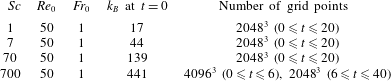
 $Sc(=1,7\text{ and }70)$ will be also given to elucidate the Schmidt-number effect (table 1).
List of non-dimensional parameters used for direct numerical simulation.

The isotropic velocity fluctuations which satisfy (2.1) are developed without stratification until enstrophy becomes maximum, and the developed flow is used as the initial condition at  $t=0$ (e.g. Staquet & Godeferd Reference Staquet and Godeferd1998; Okino & Hanazaki Reference Okino and Hanazaki2019).
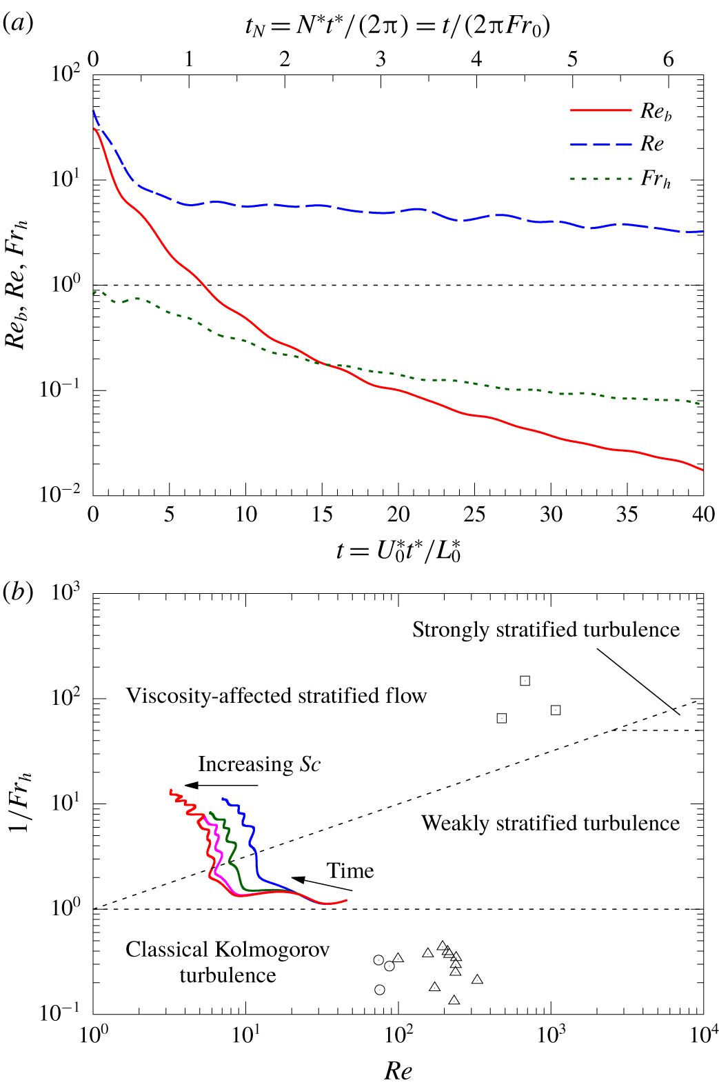
We show in figure 1(a) the temporal variation of the Reynolds number  $Re=U^{\ast 4}/(\unicode[STIX]{x1D708}^{\ast }\unicode[STIX]{x1D716}_{K}^{\ast })$, the horizontal Froude number
 $Fr_{h}=\unicode[STIX]{x1D716}_{K}^{\ast }/(N^{\ast }U^{\ast 2})$ (
 $U^{\ast }$ is the mean horizontal velocity) and the buoyancy Reynolds number
 $Re_{b}=\unicode[STIX]{x1D716}_{K}^{\ast }/(\unicode[STIX]{x1D708}^{\ast }N^{\ast 2})=ReFr_{h}^{2}$ in our simulation for
 $Sc=700$. Since the Reynolds number decreases below
 $10$ in a few eddy-turnover times, nonlinear effects would not be significant in the present simulation.
The buoyancy Reynolds number represents also the ratio between the Kolmogorov wavenumber and the Ozmidov wavenumber  $k_{O}^{\ast }(=(N^{\ast 3}/\unicode[STIX]{x1D716}_{K}^{\ast })^{1/2})$, since it can be rewritten as
 $Re_{b}=(k_{K}^{\ast }/k_{O}^{\ast })^{4/3}$. The value of
 $Re_{b}$ starts at
 $31$ and falls below unity at
 $t\sim 7$ after which time the velocity components smaller than the Kolmogorov scale begin to be affected by stratification since the Ozmidov wavenumber exceeds the Kolmogorov wavenumber.
The four regimes classified by the Reynolds number  $Re$ and the inverse horizontal Froude number
 $1/Fr_{h}$, as proposed by Brethouwer et al. (Reference Brethouwer, Billant, Lindborg and Chomaz2007), are presented in figure 1(b). The initial Reynolds number in our direct numerical simulation (
 $Re_{0}=50$) is close to the saltwater experiments by Stillinger, Helland & Van Atta (Reference Stillinger, Helland and Van Atta1983), and the initial value of
 $1/Fr_{h}({\sim}1)$ is near the border between the classical Kolmogorov turbulence and the weakly stratified turbulence. The parameters (
 $Re,1/Fr_{h}$) develop into the viscosity-affected stratified flow as the turbulence decays with time.
The parameters in the saltwater experiments by Praud et al. (Reference Praud, Fincham and Sommeria2005) belong to the viscosity-affected stratified flow from the beginning, since the initial Froude number ( $=O(10^{-2})$) is very low while the Reynolds number is large. Noting that
 $Re_{b}=ReFr_{h}^{2}$ means
 $\log 1/Fr_{h}=(1/2)\log Re-(1/2)\log Re_{b}$, the value of
 $Re_{b}$ is constant in this parameter map along a straight line with slope
 $1/2$. Then, the buoyancy Reynolds numbers at late times in our simulations (
 $Re_{b}\lesssim 10^{-1}$) are comparable to the initial values of
 $Re_{b}$ in the experiments by Praud et al. (Reference Praud, Fincham and Sommeria2005), although the Reynolds number is much smaller in our simulations.
(a) Temporal variation of the buoyancy Reynolds number  $Re_{b}=\unicode[STIX]{x1D716}_{K}^{\ast }/(\unicode[STIX]{x1D708}^{\ast }N^{\ast 2})$, the Reynolds number
 $Re=U^{\ast 4}/(\unicode[STIX]{x1D708}^{\ast }\unicode[STIX]{x1D716}_{K}^{\ast })$ and the horizontal Froude number
 $Fr_{h}=\unicode[STIX]{x1D716}_{K}^{\ast }/(N^{\ast }U^{\ast 2})$ for
 $Sc=700$. The upper abscissa indicates the buoyancy time
 $t_{N}(=N^{\ast }t^{\ast }/(2\unicode[STIX]{x03C0}))$. (b) The four regimes classified by the Reynolds number
 $Re$ and the inverse horizontal Froude number
 $1/Fr_{h}$, as proposed by Brethouwer et al. (Reference Brethouwer, Billant, Lindborg and Chomaz2007). The straight line with the slope of
 $1/2$ indicates
 $Re_{b}(=\,ReFr_{h}^{2})=1$, since
 $\log 1/Fr_{h}=(1/2)\log Re$ if
 $Re_{b}=1$. The four curves, from right to left, show the temporal variation of numerical results for
 $Sc=1,7,70$ and
 $700$. The symbols show the nearly initial parameters in previous saltwater experiments: ○, ‘run 23’ of Stillinger et al. (Reference Stillinger, Helland and Van Atta1983); ▵, ‘R36’, ‘R37’ and ‘R52’ of Itsweire et al. (Reference Itsweire, Helland and Van Atta1986); ▫, ‘ba’, ‘bb’ and ‘ia’ of Praud et al. (Reference Praud, Fincham and Sommeria2005).

To estimate the dimensional values corresponding to the non-dimensional parameters  $Re$ and
 $Fr_{h}$ considered in the numerical simulations, we use here the data in saltwater experiments by Itsweire et al. (Reference Itsweire, Helland and Van Atta1986) since the Reynolds and Froude numbers at downstream positions are similar to our initial values. For example, at
 $x^{\ast }/M^{\ast }=20$, with
 $x^{\ast }$ being the streamwise distance from the turbulence grid and
 $M^{\ast }$ the mesh size of the grid, the horizontal turbulent velocity is
 $U^{\ast }=0.6{-}0.9~(\text{cm}~\text{s}^{-1})$, the kinetic-energy dissipation rate is
 $\unicode[STIX]{x1D716}_{K}^{\ast }=0.2{-}0.5~(\text{cm}^{2}~\text{s}^{-3})$ and the Brunt–Väisälä frequency is
 $N^{\ast }=0.3{-}1.0~(\text{s}^{-1})$, giving
 $Re=55{-}160$ and
 $Fr_{h}=0.5{-}2.5$ which are comparable to our numerical simulations. Other dimensional values are the integral scale
 $L^{\ast }=U^{\ast 3}/\unicode[STIX]{x1D716}_{K}^{\ast }\sim 1~(\text{cm})$, the Kolmogorov scale
 $L_{K}^{\ast }=1/k_{K}^{\ast }\sim 0.04~(\text{cm})$, the Batchelor scale
 $L_{B}^{\ast }=1/k_{B}^{\ast }\sim 2\times 10^{-3}(\text{cm})$ and the Ozmidov scale
 $L_{O}^{\ast }=1/k_{O}^{\ast }=0.5{-}4~(\text{cm})$ (cf. table 2 of Itsweire et al. (Reference Itsweire, Helland and Van Atta1986)).
The governing equations are solved by the Fourier-spectral method in a periodic cube whose side is  $4\unicode[STIX]{x03C0}$, and the minimum wavenumber in the present computation becomes
 $k_{min}=0.5$. The aliasing errors are removed by the
 $3/2$-rule. For the highest Schmidt number of
 $Sc=700$, we used
 $4096^{3}$ grid points for the initial time development (
 $t\leqslant 6$). Then, the initial maximum resolved wavenumber becomes
 $k_{max}=682.5$, and the sufficient resolution down to the Batchelor scale is assured (
 $k_{max}/k_{B}=682.5/441=1.55$ at
 $t=0$). The grid resolution is reduced to
 $2048^{3}$ at
 $t=6$, truncating the components of
 $k>k_{max}^{\prime }\equiv 341$, where
 $k_{max}^{\prime }$ is the maximum wavenumber resolved by
 $2048^{3}$ grid points, and
 $k_{max}^{\prime }/k_{B}\geqslant 1.66$ is satisfied with
 $k_{B}=205$ at
 $t=6$. For the time development of the nonlinear and the buoyancy terms, a fourth-order Runge–Kutta method is used, while the viscosity and the diffusion terms are evaluated analytically using the integrating factor.
The numerical simulation has been executed using 1024 nodes of one of the two NEC SX-ACE systems located in the Cyberscience Center of Tohoku University or in the Earth Simulator Center of the Japan Agency of Marine-Earth Science and Technology. The execution time for the simulation of  $Sc=700$ is 113 hours for the initial period of
 $0\leqslant t\leqslant 6$ using 1024 nodes, and 109 hours for the remaining period of
 $6\leqslant t\leqslant 40$, using 256 nodes.
3 Results
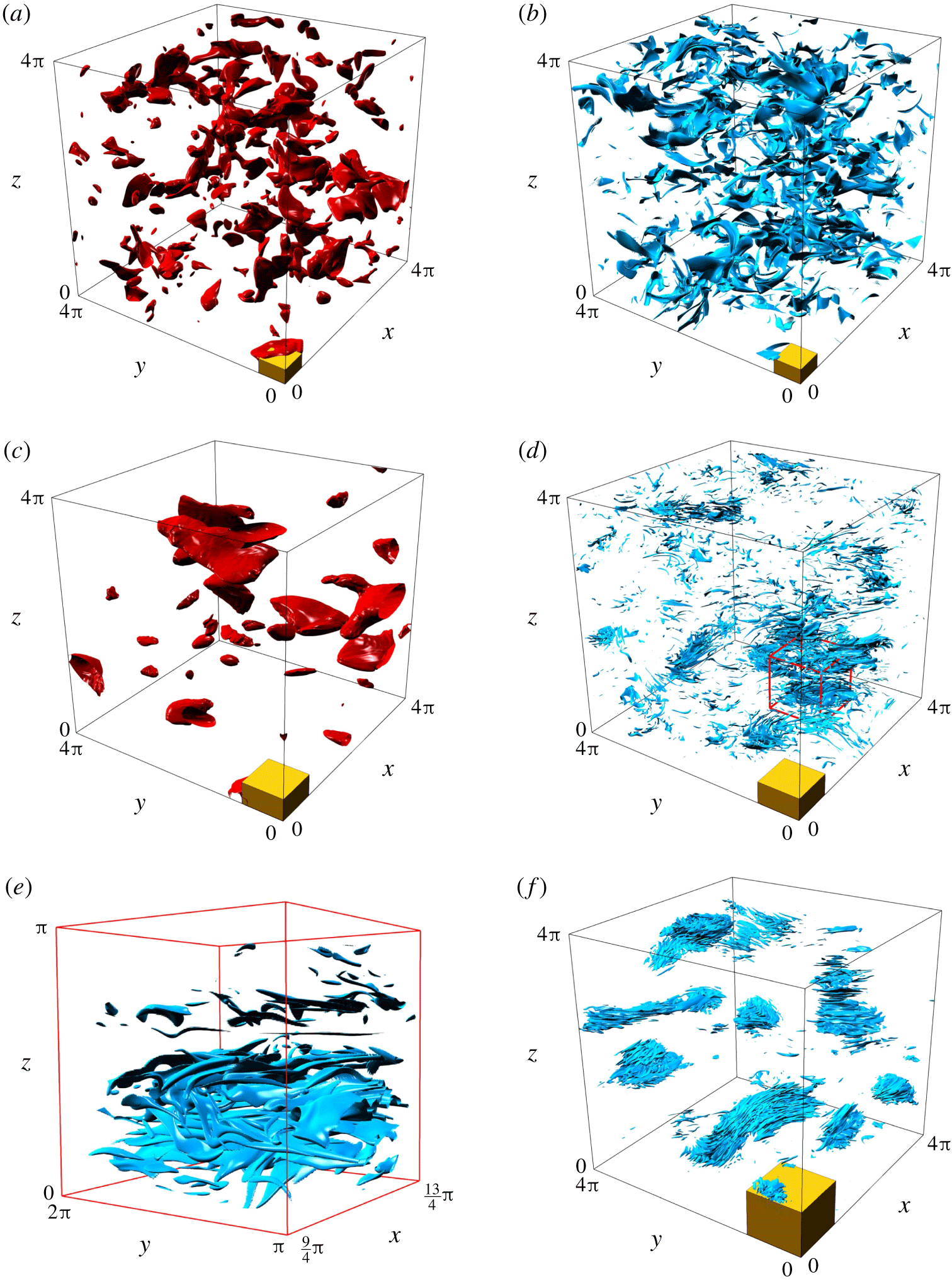
We first discuss the results for  $Sc=700$, and figure 2 shows the spatial distribution of kinetic and potential energy at three different times (
 $t=4,20$ and
 $40$). At the earliest time (
 $t=4$, figure 2a,b), the buoyancy time is still small (
 $t_{N}=N^{\ast }t^{\ast }/(2\unicode[STIX]{x03C0})=0.64({<}1)$. cf. figure 1a), and the buoyancy effect would be generally insignificant. The Ozmidov scale (
 $L_{O}=1/k_{O}=0.26$) is smaller than the horizontal and vertical integral scales (
 $L_{H}=1.4$ and
 $L_{V}=0.77$), but is still larger than the Kolmogorov scale (
 $L_{K}=1/k_{K}=0.11$), and the eddies with the Kolmogorov scale would not be strongly affected by stratification. Here, the horizontal and vertical integral scales are defined by
 $$\begin{eqnarray}L_{H}=\frac{\displaystyle \unicode[STIX]{x03C0}\int \text{d}k_{y}\int \text{d}k_{z}|\hat{u} (0,k_{y},k_{z})|^{2}}{\overline{u^{2}}}\quad \text{and}\quad L_{V}=\frac{\displaystyle \unicode[STIX]{x03C0}\int \text{d}k_{x}\int \text{d}k_{y}|{\hat{w}}(k_{x},k_{y},0)|^{2}}{\overline{w^{2}}},\end{eqnarray}$$
(e.g. Bradshaw Reference Bradshaw1971), where  $\boldsymbol{k}=(k_{x},k_{y},k_{z})$ is the wavevector, hat (
 $\hat{~}$) denotes the Fourier component and overlines denote the spatial average.
Since the Batchelor scale for a scalar of high-Schmidt-number ( $Sc=700$) is much smaller than the Kolmogorov scale (
 $L_{B}=L_{K}/Sc^{1/2}=0.004$), density has fluctuations of much smaller scales than the velocity fluctuations. It has actually a thin sheet-like structure with a thickness approximately equal to the Batchelor scale (figure 2b), as observed in isotropic turbulence for a passive scalar with mean gradient (e.g. Brethouwer, Hunt & Nieuwstadt Reference Brethouwer, Hunt and Nieuwstadt2003).
Later at  $t=20$ (figure 2c,d), the Ozmidov scale
 $L_{O}(=\,0.045)$ becomes much smaller than the Kolmogorov scale
 $L_{K}(=0.25)$, and the smallest-scale motion at
 $L_{K}$ would be significantly affected by stratification. The kinetic-energy distribution at this time shows large-scale flat structures with the horizontal and vertical integral scales of velocity given by
 $L_{H}(=2.2)$ and
 $L_{V}(=1.2)$. On the other hand, the potential-energy distribution shows large-scale clouds (figure 2d) composed of small-scale horizontal streaks, as can be identified in the enlarged view (figure 2e).
At  $t=40$ (figure 2f), most of the small-scale fluctuations of density have already dissipated, leaving only the large-scale flat structures but with smaller-scale horizontal wrinkles. Similar structures have been observed at
 $Sc=70$ (Okino & Hanazaki Reference Okino and Hanazaki2019) since a vertical scale smaller than the Kolmogorov scale is generated by a vertically sheared horizontal flow which appears in the final period of decay.
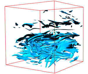
Spatial distributions of the kinetic and potential energy for  $Sc=700$ at
 $t=4,20$ and
 $40$. The isosurfaces of (a)
 $u_{i}^{2}/2=3KE$ (
 $t=4$), (b)
 $\unicode[STIX]{x1D70C}^{\prime 2}/(2Fr_{0}^{2})=8PE$ (
 $t=4$), (c)
 $u_{i}^{2}/2=3KE$ (
 $t=20$), (d)
 $\unicode[STIX]{x1D70C}^{\prime 2}/(2Fr_{0}^{2})=8PE$ (
 $t=20$) and (f)
 $\unicode[STIX]{x1D70C}^{\prime 2}/(2Fr_{0}^{2})=6PE$ (
 $t=40$), where
 $KE$ and
 $PE$ are the spatially averaged kinetic and potential energy. (e) The red cube in (d) with side
 $\unicode[STIX]{x03C0}$, which is four-times enlarged. The horizontal and vertical sizes of a yellow box at the origin
 $(0,0,0)$ in each figure indicate the horizontal and vertical integral scales.

To investigate the large- and small-scale structures of density fluctuations, we decompose the spectral components into low- and high-wavenumber components relative to the Kolmogorov wavenumber, i.e.
 $$\begin{eqnarray}\unicode[STIX]{x1D70C}_{L}^{\prime }(\boldsymbol{x})=\mathop{\sum }_{|\boldsymbol{k}|\leqslant k_{K}}\hat{\unicode[STIX]{x1D70C}^{\prime }}(\boldsymbol{k})\exp (\text{i}\boldsymbol{k}\boldsymbol{\cdot }\boldsymbol{x})\quad \text{and}\quad \unicode[STIX]{x1D70C}_{H}^{\prime }(\boldsymbol{x})=\mathop{\sum }_{|\boldsymbol{k}|>k_{K}}\hat{\unicode[STIX]{x1D70C}^{\prime }}(\boldsymbol{k})\exp (\text{i}\boldsymbol{k}\boldsymbol{\cdot }\boldsymbol{x}),\end{eqnarray}$$
where
 $$\begin{eqnarray}\unicode[STIX]{x1D70C}^{\prime }(\boldsymbol{x})=\unicode[STIX]{x1D70C}_{L}^{\prime }(\boldsymbol{x})+\unicode[STIX]{x1D70C}_{H}^{\prime }(\boldsymbol{x}).\end{eqnarray}$$
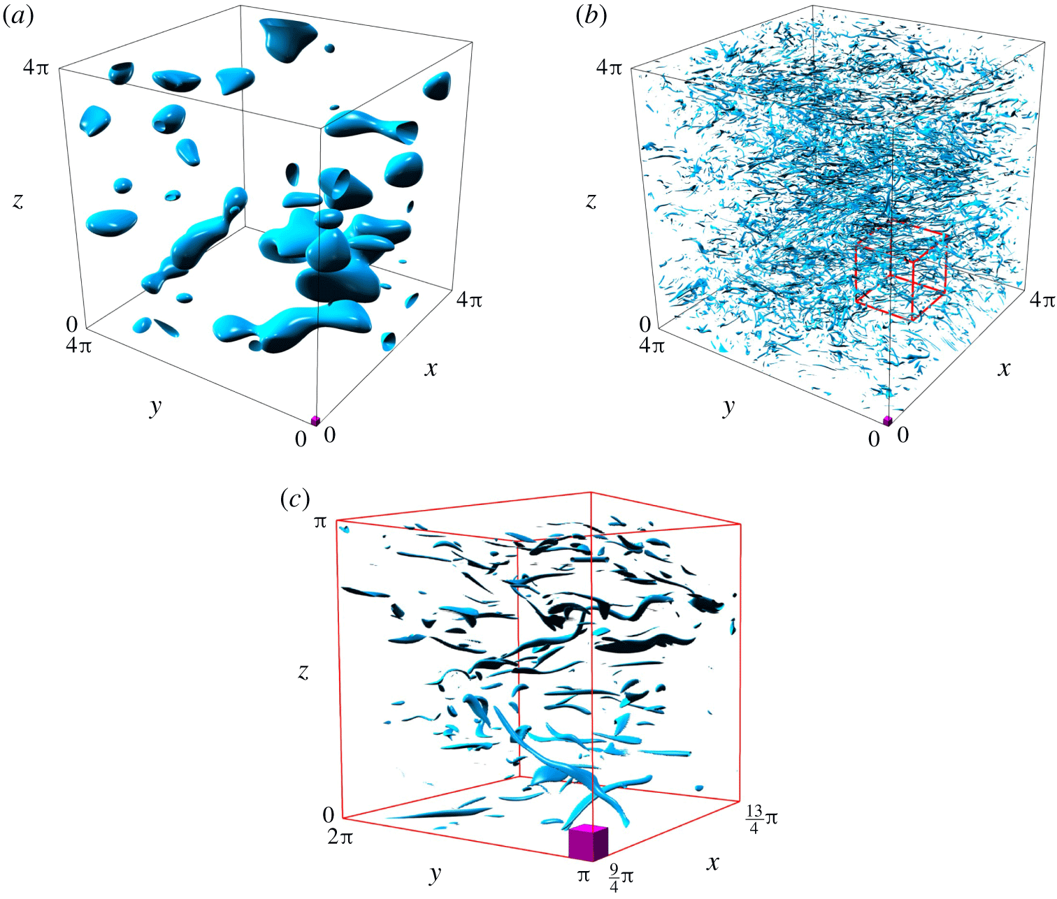
In figure 3(a,b), we show the distributions of potential energy at  $t=20$, composed only of low or high wavenumbers. The low-wavenumber components constitute round structures (figure 3a), while the high-wavenumber components constitute long horizontal streaks, whose cross-section is vertically thin (figure 3b,c). We note that neither the low-wavenumber components (figure 3a) nor the high-wavenumber components (figure 3b,c) have a noticeable structure of the Kolmogorov scale (
 $L_{K}=0.25$), which is indicated by the side of a pink box. The absence of potential energy near the Kolmogorov scale will be demonstrated later, using premultiplied energy spectra (cf. figures 6d and 11b).
Spatial distributions of potential energy for  $Sc=700$ at
 $t=20$, composed only of low (
 $|\boldsymbol{k}|\leqslant k_{K}$) or high (
 $|\boldsymbol{k}|>k_{K}$) wavenumbers. Isosurfaces of (a)
 $\unicode[STIX]{x1D70C}_{L}^{\prime 2}/(2Fr_{0}^{2})=3PE$ and (b)
 $\unicode[STIX]{x1D70C}_{H}^{\prime 2}/(2Fr_{0}^{2})=3PE$. (c) The red cube in (b) with side
 $\unicode[STIX]{x03C0}$, which is four-times enlarged. The sum of (a,b) does not recover the local distribution of
 $\unicode[STIX]{x1D70C}^{\prime 2}/(2Fr_{0}^{2})$ like figure 2(d), since
 $\unicode[STIX]{x1D70C}^{\prime 2}=(\unicode[STIX]{x1D70C}_{L}^{\prime }+\unicode[STIX]{x1D70C}_{H}^{\prime })^{2}=\unicode[STIX]{x1D70C}_{L}^{\prime 2}+\unicode[STIX]{x1D70C}_{H}^{\prime 2}+2\unicode[STIX]{x1D70C}_{L}^{\prime }\unicode[STIX]{x1D70C}_{H}^{\prime }$, and contribution from
 $2\unicode[STIX]{x1D70C}_{L}^{\prime }\unicode[STIX]{x1D70C}_{H}^{\prime }/(2Fr_{0}^{2})$ is lacking. However,
 $\unicode[STIX]{x1D70C}_{L}^{\prime }\unicode[STIX]{x1D70C}_{H}^{\prime }$ does not contribute to
 $PE$ since
 $\overline{\unicode[STIX]{x1D70C}_{L}^{\prime }\unicode[STIX]{x1D70C}_{H}^{\prime }}=0$, and
 $PE=\overline{\unicode[STIX]{x1D70C}^{\prime 2}}/(2Fr_{0}^{2})=(\overline{\unicode[STIX]{x1D70C}_{L}^{\prime 2}}+\overline{\unicode[STIX]{x1D70C}_{H}^{\prime 2}})/(2Fr_{0}^{2})$. The size of the pink box at the bottom represents the Kolmogorov scale
 $L_{K}=1/k_{K}=0.25$.

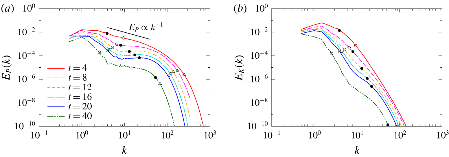
Figure 4(a,b) shows a time development of the radial spectra of potential energy and kinetic energy,  $E_{P}(k)$ and
 $E_{K}(k)$, for
 $Sc=700$. Since the potential energy is zero at
 $t=0$, kinetic energy is initially converted to potential energy through the vertical density flux due to the buoyancy (cf. figure 8). The potential energy is then cascaded to high wavenumbers at the same time as the energy is converted from the kinetic energy, and a potential-energy spectrum proportional to
 $k^{-1}$ is generated near the Kolmogorov wavenumber before the vertical density flux oscillates once (
 $t=4$). This initial spectrum is similar to a variance spectrum of a passive scalar of
 $Sc\gg 1$ in isotropic turbulence (Batchelor Reference Batchelor1959).
However, the potential energy decays with time, and bending of the spectrum appears at  $t=8$. At the same time, the spectrum becomes flat at wavenumbers higher than the wavenumber at which the spectrum bends, which is approximately
 $k=7$ for the period of
 $8\leqslant t\leqslant 20$.
In decaying turbulence where  $\unicode[STIX]{x1D716}_{K}$ decreases with time, the Kolmogorov and Batchelor wavenumbers decrease with time, while the Ozmidov wavenumber increases. Thus, the Kolmogorov wavenumber and the Ozmidov wavenumber coincide (
 $k_{K}^{\ast }=k_{O}^{\ast }$) at the primitive wavenumber of stratified turbulence
 $k_{P}^{\ast }=\sqrt{N^{\ast }/\unicode[STIX]{x1D708}^{\ast }}$ (Gibson Reference Gibson and Nihoul1980) in due course. In the present numerical simulations, its non-dimensional value is
 $k_{P}=\sqrt{N^{\ast }/\unicode[STIX]{x1D708}^{\ast }}L_{0}^{\ast }=(Re_{0}/Fr_{0})^{1/2}=(50/1)^{1/2}=7.1$. Therefore, as far as we can identify from figure 4(a), the bend of the spectrum appears near the primitive wavenumber.
The primitive wavenumber  $k_{P}$ is constant in time since it is determined by the stratification
 $N^{\ast }$ and the viscosity
 $\unicode[STIX]{x1D708}^{\ast }$. Also,
 $k_{P}$ does not change with the Schmidt number
 $Sc$ (figure 5) since it is independent of the diffusion coefficient of density
 $\unicode[STIX]{x1D705}^{\ast }$. Furthermore, the definition of this wavenumber contains neither the total amount of kinetic energy nor the kinetic-energy dissipation rate
 $\unicode[STIX]{x1D716}_{K}^{\ast }$ which is related to the rate of the energy cascade per unit time, so it is not affected by nonlinear effects.
The corresponding kinetic-energy spectrum  $E_{K}(k)$ also decreases with time (figure 4b), and bends near
 $k_{P}$ after a long time (
 $t\geqslant 16$). This occurs since the local decrease of potential energy near
 $k_{P}$ leads to the reduction of energy conversion into kinetic energy via the vertical density flux also near
 $k_{P}$.
Temporal variation of (a) potential-energy spectrum  $E_{P}(k)$ and (b) kinetic-energy spectrum
 $E_{K}(k)$ for
 $Sc=700$. Symbols on each spectral line show Kolmogorov wavenumber (○), Ozmidov wavenumber (●) and Batchelor wavenumber (▵).

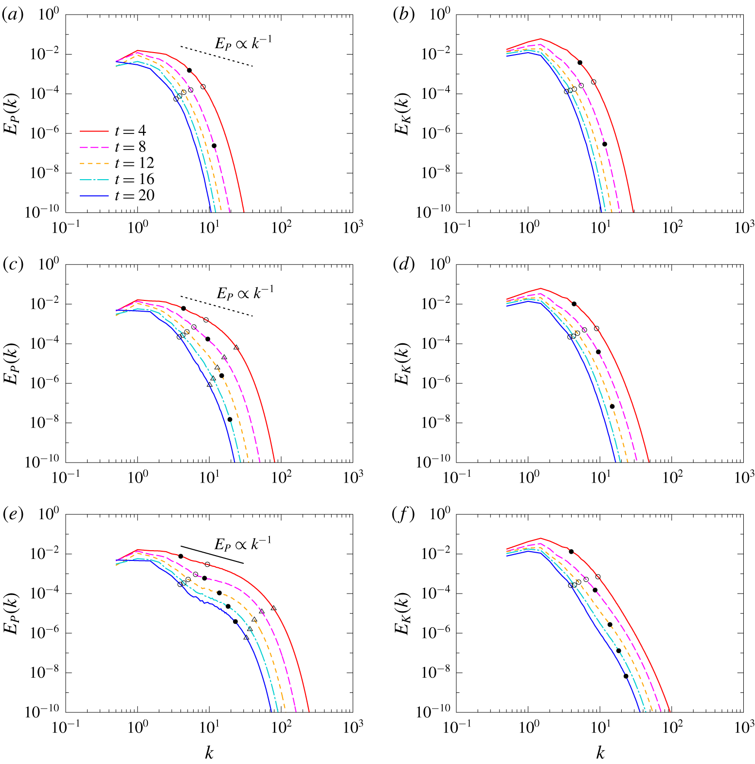
Such bending of the spectrum has not been observed in the previous numerical simulations of stratified turbulence at lower Schmidt numbers ( $Sc\lesssim 7$). We show in figure 5 the Schmidt number dependence of the potential-energy spectrum (
 $Sc=1,7$ and
 $70$). When
 $Sc=1$ (figure 5a,b),
 $E_{P}(k)$ and
 $E_{K}(k)$ dissipate at the same wavenumber since the Kolmogorov and Batchelor scales are the same, and their spectral shapes are very similar at wavenumbers larger than
 $k_{K}$.
When  $Sc=7({>}1)$ (figure 5c,d),
 $k_{K}<k_{B}$ holds, and the dissipation of potential energy occurs at wavenumbers larger than
 $k_{K}$, and
 $E_{P}(k)$ differs from
 $E_{K}(k)$ at high wavenumbers. However, neither the bending nor the plateau of the spectrum are observed yet for
 $Sc\leqslant 7$. Since the potential energy initially cascades to wavenumbers larger than the Kolmogorov wavenumber, the kinetic energy at high wavenumbers also increases through the energy conversion by the vertical density flux, compared to the case of
 $Sc=1$ (cf. figure 5b,d).
In contrast, when  $Sc$ increases to 70 (figure 5e), the potential energy spectrum
 $E_{P}(k)$ shows the
 $k^{-1}$ spectrum near the Kolmogorov wavenumber at
 $t=4$, due to the initial energy cascade (Batchelor Reference Batchelor1959). After this time, a weak bending of
 $E_{P}(k)$ is observed as time progresses. The same trend could be observed in the numerical simulation for
 $Re_{0}=100$ (Okino & Hanazaki Reference Okino and Hanazaki2019, figure 13d), although the bending of the spectrum was not discussed there. The potential-energy spectrum bends at
 $k\sim 7$, approximately the same value as the case of
 $Sc=700$. The independence of this wavenumber from the Schmidt number
 $Sc$ supports the possibility that this wavenumber is equal to the primitive wavenumber
 $k_{P}$ determined only by
 $N^{\ast }$ and
 $\unicode[STIX]{x1D708}^{\ast }$ (or
 $Fr_{0}$ and
 $Re_{0}$). However, the bending at
 $Sc=70$ is weaker than
 $Sc=700$, and thus the spectrum does not become flat at high wavenumbers, since the initial potential-energy transfer to high wavenumbers is smaller due to larger molecular diffusion of density.
Temporal variation of potential-energy spectrum  $E_{P}(k)$ and kinetic-energy spectrum
 $E_{K}(k)$. (a)
 $E_{P}(k)$ for
 $Sc=1$; (b)
 $E_{K}(k)$ for
 $Sc=1$; (c)
 $E_{P}(k)$ for
 $Sc=7$; (d)
 $E_{K}(k)$ for
 $Sc=7$; (e)
 $E_{P}(k)$ for
 $Sc=70$; (f)
 $E_{K}(k)$ for
 $Sc=70$. Symbols on each spectral line show Kolmogorov wavenumber (○), Ozmidov wavenumber (●) and Batchelor wavenumber (▵).

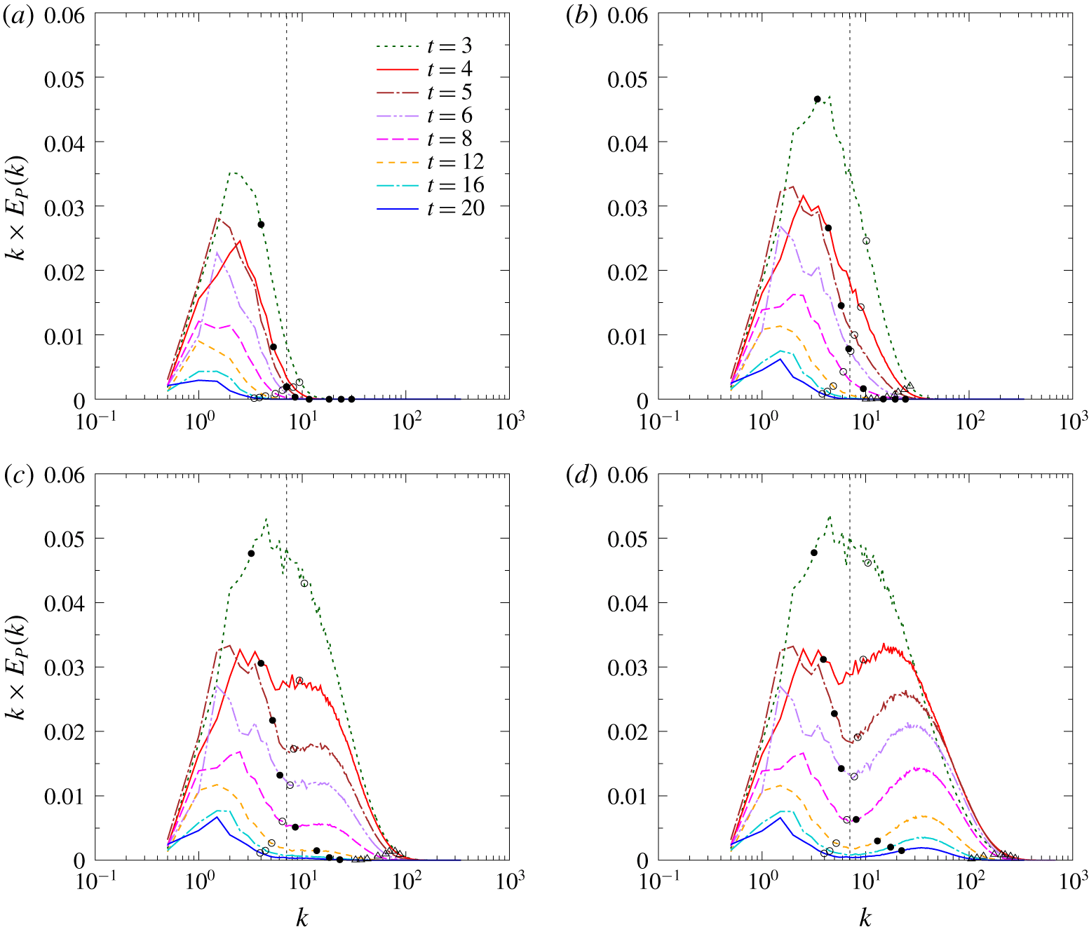
Temporal variation of the premultiplied potential-energy spectrum  $k\times E_{P}(k)$ for (a)
 $Sc=1$, (b)
 $Sc=7$, (c)
 $Sc=70$ and (d)
 $Sc=700$. Symbols on each spectral line show Kolmogorov wavenumber (○), Ozmidov wavenumber (●) and Batchelor wavenumber (▵). The vertical dotted lines indicate the primitive wavenumber
 $k_{P}=\sqrt{50}\simeq 7.1$.

When the energy spectrum  $E_{P}(k)$ is multiplied by wavenumber
 $k$ and plotted against
 $\log k$, the area below the line of
 $kE_{P}(k)$ indicates the amount of potential energy. Such a spectrum is often called ‘premultiplied spectrum’ (e.g. Perry, Henbest & Chong Reference Perry, Henbest and Chong1986), and we use it here to visualise the amount of energy in a specific range of wavenumbers. We then show the time development of the premultiplied spectrum of potential energy
 $kE_{P}(k)$ in figure 6 to discuss the variation of potential energy at specific wavenumbers.
When  $Sc=1$ (figure 6a), i.e.
 $\unicode[STIX]{x1D705}^{\ast }=\unicode[STIX]{x1D708}^{\ast }$, the Kolmogorov scale is equal to the Batchelor scale, and the potential energy also dissipates near the Kolmogorov wavenumber (○). The total amount of potential energy is small compared to the other cases of
 $Sc(=7,70\text{ and }700)$ shown in figure 6(b–d), since the molecular diffusion of density is large.
When the Schmidt number increases to  $Sc=7$ (figure 6b), a certain amount of potential energy exists below the Kolmogorov scale since
 $k_{B}/k_{K}=\sqrt{7}\simeq 2.6$.
When  $Sc=70$ (figure 6c), the viscous-convective subrange becomes broader (
 $k_{B}/k_{K}=\sqrt{70}\simeq 8.4$), and a relatively flat spectrum or a plateau appears initially (
 $t\sim 4$), corresponding to the appearance of the
 $k^{-1}$ spectrum in
 $E_{P}(k)$ (figure 5e). Later, a significant decrease is observed near the primitive wavenumber
 $k_{P}$ (vertical dotted line), where
 $k_{O}$ and
 $k_{K}$ agree.
When the Schmidt number further increases up to  $Sc=700$ (figure 6d), a plateau appears initially (
 $t=3{-}4$), again corresponding to the appearance of the
 $k^{-1}$ law in
 $E_{P}(k)$ (figure 4a). Subsequently, the potential energy decreases locally near the primitive wavenumber, and two peaks are formed at low and high wavenumbers. Unlike the case of
 $Sc=70$, the peak at the higher wavenumber is large since the Batchelor wavenumber (
 $k_{B}$) is 26 times larger than
 $k_{K}$ and the significant portion of potential energy initially exists below the Kolmogorov scale. The peak at the lower wavenumber (
 $k\sim 1.5$) corresponds to the large-scale round structures observed in figure 3(a), while the peak at the higher wavenumber (
 $k\sim 40$) corresponds to the small-scale horizontal streaks observed in figure 3(b,c).
The total amount of potential energy  $PE(=\overline{\unicode[STIX]{x1D70C}^{\prime 2}}/(2Fr_{0}^{2}))$ increases significantly with
 $Sc$ since the molecular dissipation becomes smaller for a smaller diffusion coefficient (cf. figures 2a and 5 of Okino & Hanazaki (Reference Okino and Hanazaki2019) for
 $Sc=1,7$ and
 $70$). This can be identified here also for
 $Sc=700$, by the increase of the area below the curves of
 $kE_{P}(k)$. On the other hand, the total amount of kinetic energy
 $KE(=\overline{u_{i}^{2}}/2)$ is rather insensitive to
 $Sc$, since the effects of a large Schmidt number are limited mainly to small scales below the Kolmogorov scale (figures 4b and 5b,d,f). Therefore, the energy ratio
 $PE/KE$ becomes larger for larger
 $Sc$.
To investigate the origin of the significant decrease of potential energy near the primitive wavenumber, we consider the budget for the potential-energy spectrum, i.e.
 $$\begin{eqnarray}\frac{\unicode[STIX]{x2202}E_{P}(k)}{\unicode[STIX]{x2202}t}=-D_{P}(k)+C_{\unicode[STIX]{x1D70C}^{\prime }w}(k)+T_{P}(k),\end{eqnarray}$$
where  $D_{P}(k)$ is the potential-energy dissipation spectrum,
 $$\begin{eqnarray}D_{P}(k)=\mathop{\sum }_{\left|\sqrt{k_{x}^{2}+k_{y}^{2}+k_{z}^{2}}-k\right|<k_{min}/2}\frac{k_{j}^{2}}{Re_{0}ScFr_{0}^{2}}\big|\hat{\unicode[STIX]{x1D70C}^{\prime }}(k_{x},k_{y},k_{z})\big|^{2}\frac{1}{k_{min}},\end{eqnarray}$$
 $C_{\unicode[STIX]{x1D70C}^{\prime }w}(k)$ is the cospectrum of the vertical density flux responsible for the exchange between the kinetic and potential energies,
 $$\begin{eqnarray}C_{\unicode[STIX]{x1D70C}^{\prime }w}(k)=\mathop{\sum }_{\left|\sqrt{k_{x}^{2}+k_{y}^{2}+k_{z}^{2}}-k\right|<k_{min}/2}\frac{1}{Fr_{0}^{2}}\text{ Re}[\hat{\unicode[STIX]{x1D70C}^{\prime }}(k_{x},k_{y},k_{z}){\hat{w}}^{\ast }(k_{x},k_{y},k_{z})]\frac{1}{k_{min}},\end{eqnarray}$$
and  $T_{P}(k)$ is the nonlinear potential-energy transfer spectrum,
 $$\begin{eqnarray}T_{P}(k)=\mathop{\sum }_{\left|\sqrt{k_{x}^{2}+k_{y}^{2}+k_{z}^{2}}-k\right|<k_{min}/2}\frac{k_{j}}{Fr_{0}^{2}}\text{ Im}[\hat{\unicode[STIX]{x1D70C}^{\prime }}^{\ast }(k_{x},k_{y},k_{z})\widehat{\unicode[STIX]{x1D70C}^{\prime }u_{j}}(k_{x},k_{y},k_{z})]\frac{1}{k_{min}}.\end{eqnarray}$$
Its counterpart for the kinetic-energy spectrum is
 $$\begin{eqnarray}\frac{\unicode[STIX]{x2202}E_{K}(k)}{\unicode[STIX]{x2202}t}=-D_{K}(k)-C_{\unicode[STIX]{x1D70C}^{\prime }w}(k)+T_{K}(k),\end{eqnarray}$$
where  $D_{K}(k)$ is the kinetic-energy dissipation spectrum,
 $$\begin{eqnarray}D_{K}(k)=\mathop{\sum }_{\left|\sqrt{k_{x}^{2}+k_{y}^{2}+k_{z}^{2}}-k\right|<k_{min}/2}\frac{k_{j}^{2}}{Re_{0}}|\hat{u} _{i}(k_{x},k_{y},k_{z})|^{2}\frac{1}{k_{min}},\end{eqnarray}$$
and  $T_{K}(k)$ is the kinetic-energy transfer spectrum,
 $$\begin{eqnarray}T_{K}(k)=\mathop{\sum }_{\left|\sqrt{k_{x}^{2}+k_{y}^{2}+k_{z}^{2}}-k\right|<k_{min}/2}k_{j}\text{ Im}[\hat{u} _{i}^{\ast }(k_{x},k_{y},k_{z})\widehat{u_{i}u_{j}}(k_{x},k_{y},k_{z})]\frac{1}{k_{min}}.\end{eqnarray}$$
Here, the asterisk in (3.6), (3.7) and (3.10) denotes the complex conjugate.
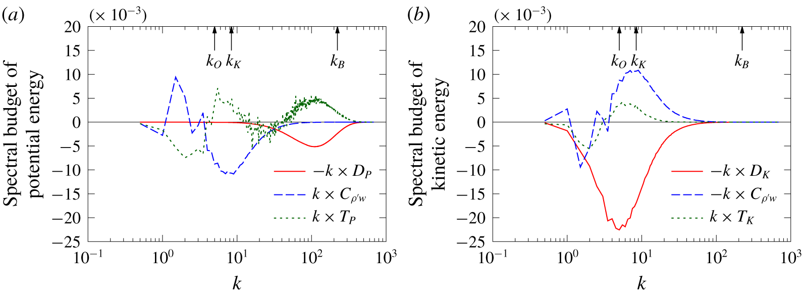
We first consider the budget for the potential energy. The three terms on the right-hand side of (3.4) are presented in their premultiplied forms in figure 7(a) for  $Sc=700$ at the time of
 $t=5$, i.e. when the local minimum near the primitive wavenumber
 $k_{P}$ is observed in the potential energy spectrum (cf. figure 6d). The potential-energy dissipation
 $-kD_{P}(k)$ has a negative peak near the Batchelor wavenumber (
 $k\sim 10^{2}$), and it counterbalances with the potential-energy transfer
 $kT_{P}(k)$. Near the primitive wavenumber
 $k_{P}(=7.1)$, vertical density flux
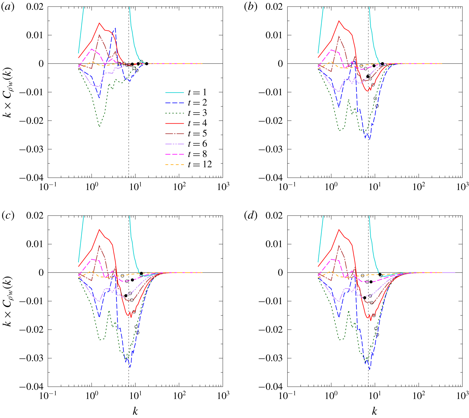
 $kC_{\unicode[STIX]{x1D70C}^{\prime }w}(k)$ is negative and counter-gradient, and this causes the local reduction of potential energy observed in figure 6(d). Indeed, the density flux is persistently counter-gradient near
 $k_{P}$, while it oscillates in time and changes sign at low wavenumbers. This behaviour will be discussed later in figure 9(d).
The spectral budget of (a) the potential energy and (b) the kinetic energy for  $Sc=700$ at
 $t=5$. The three arrows at the top of the figure indicate the Ozmidov, Kolmogorov and Batchelor wavenumbers.

We next consider the budget for the kinetic energy. The three terms on the right-hand side of (3.8) are presented in their premultiplied forms in figure 7(b). Above the primitive wavenumber, the counter-gradient density flux  $-kC_{\unicode[STIX]{x1D70C}^{\prime }w}(k)>0$ cancels with the kinetic-energy dissipation
 $-kD_{K}(k)$, and prevents the decrease of kinetic energy.
Temporal variation of the vertical density flux  $\overline{\unicode[STIX]{x1D70C}^{\prime }w}/Fr_{0}^{2}$. The upper abscissa indicates the buoyancy time
 $t_{N}(=N^{\ast }t^{\ast }/(2\unicode[STIX]{x03C0}))$.

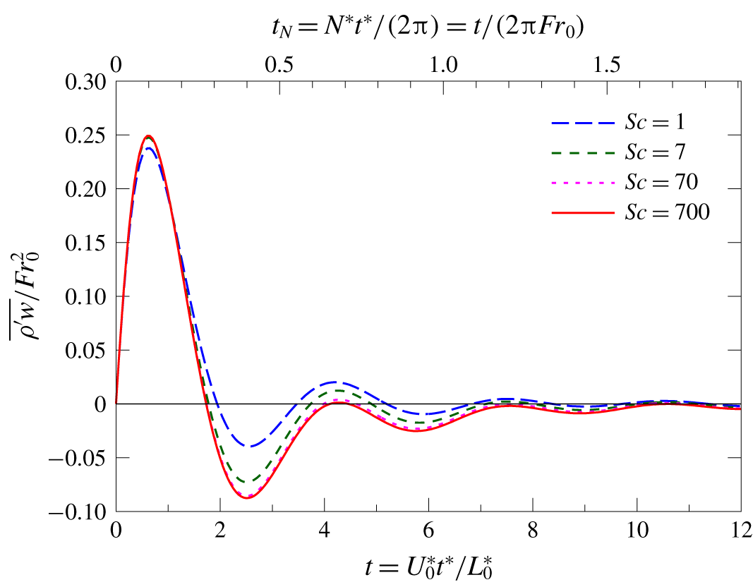
Figure 8 shows the temporal variation of the vertical density flux  $\overline{\unicode[STIX]{x1D70C}^{\prime }w}/Fr_{0}^{2}(=\int _{0}^{\infty }C_{\unicode[STIX]{x1D70C}^{\prime }w}(k)\,\text{d}k)$. Since the density perturbation is initially absent in this study, kinetic energy is converted to potential energy at early times (
 $t\lesssim 2$), through the positive vertical density flux. After that, the vertical density flux oscillates due to the buoyancy effect, at a frequency approximately twice the Brunt–Väisälä frequency (Métais & Herring Reference Métais and Herring1989; Gerz & Yamazaki Reference Gerz and Yamazaki1993), which is fundamentally a linear effect (Hanazaki & Hunt Reference Hanazaki and Hunt1996).
Since it takes some time before the effect of molecular diffusion appears, the initial temporal development of the vertical density flux does not depend on  $Sc$. However, after a while (
 $t\gtrsim 2$), stronger counter-gradient fluxes (
 $\overline{\unicode[STIX]{x1D70C}^{\prime }w}/Fr_{0}^{2}<0$) appear at larger Schmidt numbers. This is in agreement with the previous wind tunnel experiments for temperature stratification (
 $Sc=0.7$, Lienhard & Van Atta (Reference Lienhard and Van Atta1990)), water tank experiments for temperature stratification and salt stratification (
 $Sc=6$ and
 $600$, Komori & Nagata (Reference Komori and Nagata1996)), and the prediction by the rapid distortion theory (Hanazaki & Hunt Reference Hanazaki and Hunt1996). The vertical density fluxes at
 $Sc=70$ and
 $Sc=700$ are almost the same since they are determined mainly by the large-scale density perturbation and the vertical velocity, and are hardly affected by the spectral difference below the Kolmogorov scale (figures 4a and 5e).
The initial behaviour of the vertical density flux depends largely on the initial conditions such as the initial energy ratio  $PE/KE$, as investigated previously by the rapid distortion theory (Hanazaki & Hunt Reference Hanazaki and Hunt1996). For example, the initial amplitude of the vertical density flux becomes maximum when
 $PE/KE=0$ or
 $\infty$ since the initial energy conversion between
 $KE$ and
 $PE$ becomes largest, while it becomes zero when
 $PE/KE=1/2$. However, after a sufficient time necessary for the energy exchange (i.e.
 $t_{N}=N^{\ast }t^{\ast }/(2\unicode[STIX]{x03C0})\gtrsim 1$) and the energy cascade (i.e.
 $t\gtrsim 1$) has passed, we can expect spectral behaviours similar to those observed in this study, at least at small scales.
Temporal variation of the cospectrum of the vertical density flux in the premultiplied form  $k\times C_{\unicode[STIX]{x1D70C}^{\prime }w}(k)$ for (a)
 $Sc=1$, (b)
 $Sc=7$, (c)
 $Sc=70$ and (d)
 $Sc=700$. Open circle shows the Kolmogorov wavenumber, and closed circle shows the Ozmidov wavenumber at
 $t=6,8$ and
 $12$. The vertical dotted line indicates the primitive wavenumber
 $k_{P}=\sqrt{50}\simeq 7.1$.

Figure 9 shows the temporal variation of the premultiplied cospectra of the vertical density flux ( $kC_{\unicode[STIX]{x1D70C}^{\prime }w}(k)$). Since kinetic energy is converted to potential energy at early times,
 $kC_{\unicode[STIX]{x1D70C}^{\prime }w}(k)$ initially (
 $t\sim 1$) takes a positive maximum near
 $k=2$, corresponding to the initial peak wavenumber or the integral scale of the kinetic-energy spectrum. The effects of molecular viscosity and molecular diffusion are small at low wavenumbers, and it takes some time before they begin to affect the high-wavenumber components. Therefore,
 $kC_{\unicode[STIX]{x1D70C}^{\prime }w}$ at
 $t=1$ exhibits almost the same behaviour for all the Schmidt numbers except for high wavenumbers (
 $k\lesssim 10$). As a result,
 $\overline{\unicode[STIX]{x1D70C}^{\prime }w}/Fr_{0}^{2}({>}0)$ does not depend largely on
 $Sc$ at
 $t\lesssim 1$ (figure 8).
Subsequently, the low wavenumber components of the cospectrum ( $k\lesssim 4$) oscillate around zero along with the exchange of kinetic energy and potential energy, corresponding to the oscillation of
 $\overline{\unicode[STIX]{x1D70C}^{\prime }w}/Fr_{0}^{2}$ (figure 8). The low-wavenumber components of the cospectra are not affected by
 $Sc$, and no significant difference is found among
 $Sc=1,7,70$ and
 $700$, since the viscosity and the diffusivity are not effective at low wavenumbers. Nevertheless, the amplitude at low wavenumbers decreases with time, not only because the energy is transferred to higher wavenumbers, but also because the components other than the horizontal wavevector cease to contribute to the cospectrum (Hanazaki & Hunt Reference Hanazaki and Hunt1996). The latter mechanism explains why the vertical density flux
 $\overline{\unicode[STIX]{x1D70C}^{\prime }w}/Fr_{0}^{2}$ decays with oscillation, even in the absence of viscosity, diffusivity and nonlinearity.
On the other hand, the behaviour of the components with  $k\gtrsim 4$ is highly affected by
 $Sc$. When
 $Sc=1$ (figure 9a), the sign of the cospectrum changes almost simultaneously at all the wavenumbers (Gerz & Yamazaki Reference Gerz and Yamazaki1993), but when
 $Sc\geqslant 7$ (figure 9b–d), the high wavenumber components do not oscillate and are persistently negative (i.e. counter-gradient flux). The amplitude of the counter-gradient flux increases with
 $Sc$ in agreement with
 $\overline{\unicode[STIX]{x1D70C}^{\prime }w}/Fr_{0}^{2}$, although it decreases monotonically in its time development. The difference between
 $kC_{\unicode[STIX]{x1D70C}^{\prime }w}(k)$ at
 $Sc=70$ and that at
 $Sc=700$ is small, reflecting that
 $E_{K}(k)$ and
 $E_{P}(k)$ at low wavenumbers (
 $k\lesssim 10$) do not change with high Schmidt numbers (figures 4a,b and 5e,f).
The wavenumber at which the counter-gradient flux becomes strongest is almost steady, and is close to the primitive wavenumber of stratified turbulence ( $k_{P}=7.1$). At small times when
 $t\lesssim 7$, the Ozmidov wavenumber
 $k_{O}$ is smaller than
 $k_{P}$, and the nonlinear effects still exist at wavenumbers where the counter-gradient flux occurs. However, we consider here tentatively why the counter-gradient flux is strong near
 $k_{P}$, using the linear rapid distortion theory. Using the three-dimensional spectrum
 $\unicode[STIX]{x1D6F7}_{\unicode[STIX]{x1D70C}^{\prime }w}(\boldsymbol{k})$, the cospectrum can be written as
 $$\begin{eqnarray}C_{\unicode[STIX]{x1D70C}^{\prime }w}(k)=2\unicode[STIX]{x03C0}k^{2}\int _{0}^{\unicode[STIX]{x03C0}}\text{d}\unicode[STIX]{x1D703}\sin \unicode[STIX]{x1D703}\unicode[STIX]{x1D6F7}_{\unicode[STIX]{x1D70C}^{\prime }w}(k,\unicode[STIX]{x1D703}),\end{eqnarray}$$
where  $\unicode[STIX]{x1D703}$ is the angle between the wavevector and the vertical axis. Although
 $\unicode[STIX]{x1D6F7}_{\unicode[STIX]{x1D70C}^{\prime }w}$ has the time oscillating terms in the form of
 $\sin \unicode[STIX]{x1D6FC}^{\ast }t^{\ast }$ or
 $\cos \unicode[STIX]{x1D6FC}^{\ast }t^{\ast }$ where
 $$\begin{eqnarray}\unicode[STIX]{x1D6FC}^{\ast }=(4N^{\ast 2}\sin ^{2}\unicode[STIX]{x1D703}-(\unicode[STIX]{x1D708}^{\ast }-\unicode[STIX]{x1D705}^{\ast })^{2}k^{\ast 4})^{1/2},\end{eqnarray}$$
only the components of  $\unicode[STIX]{x1D703}\sim \unicode[STIX]{x03C0}/2$ tend to contribute to the
 $\unicode[STIX]{x1D703}$-integral in (3.11) as time progresses (Hanazaki & Hunt Reference Hanazaki and Hunt1996). Since
 $\sin \unicode[STIX]{x1D6FC}^{\ast }t^{\ast }$ approaches
 $\sin ((4N^{\ast 2}-(\unicode[STIX]{x1D708}^{\ast }-\unicode[STIX]{x1D705}^{\ast })^{2}k^{\ast 4})^{1/2}t^{\ast })$ in the limit of
 $\unicode[STIX]{x1D703}\rightarrow \unicode[STIX]{x03C0}/2$, the integral (3.11) oscillates in time when
 $4N^{\ast 2}-(\unicode[STIX]{x1D708}^{\ast }-\unicode[STIX]{x1D705}^{\ast })^{2}k^{\ast 4}>0$, i.e. in the wavenumber range of
 $k^{\ast }<\sqrt{2N^{\ast }/|\unicode[STIX]{x1D708}^{\ast }-\unicode[STIX]{x1D705}^{\ast }|}$. Therefore,
 $k_{c}^{\ast }=\sqrt{2N^{\ast }/|\unicode[STIX]{x1D708}^{\ast }-\unicode[STIX]{x1D705}^{\ast }|}$ is the critical wavenumber between the decaying oscillation and the monotonic decay. In non-dimensional form, the wavenumber becomes
 $$\begin{eqnarray}k_{c}=\left(\frac{2Re_{0}}{Fr_{0}}\frac{1}{\left|1-{\displaystyle \frac{1}{Sc}}\right|}\right)^{1/2}.\end{eqnarray}$$
This expression shows that, when  $Sc=1$,
 $k_{c}$ becomes infinity and the cospectrum oscillates in time at all the wavenumbers. On the other hand, when
 $Sc\gg 1$, the critical wavenumber can be approximated by
 $$\begin{eqnarray}k_{c}\simeq \left(\frac{2Re_{0}}{Fr_{0}}\right)^{1/2}=\sqrt{2}k_{P}.\end{eqnarray}$$
This value is close to the primitive wavenumber  $k_{P}$, and
 $k_{c}\simeq 10$ in the present study. Figure 9 shows that the zero of
 $kC_{\unicode[STIX]{x1D70C}^{\prime }w}(k)$ is at around
 $k=4$, and is smaller than
 $k_{c}=10$. However, the graph of cospectrum will move downward due to the persistently negative components which are significant at high wavenumbers (cf. (4.9) of Hanazaki & Hunt (Reference Hanazaki and Hunt1996)). Thus, the point of zero can move toward a lower wavenumber, and will partly explain the difference between
 $k=4$ and
 $k_{c}=10$.
Another explanation for the possible importance of  $k_{P}$ is that it is near the Kolmogorov wavenumber. In decaying turbulence,
 $k_{K}$ decreases with time while
 $k_{O}$ increases with time, and they agree at
 $k_{P}$ when
 $t\simeq 7$. Then, the Kolmogorov wavenumber is not far from the primitive wavenumber at which the strong counter-gradient flux is observed. On the other hand, since the vertical density flux is the product of
 $\unicode[STIX]{x1D70C}^{\prime }$ and
 $w$, it decreases significantly for
 $k\gtrsim k_{K}$, where
 $w$ decreases. Then, a strong counter-gradient flux could be observed just above the Kolmogorov scale. This may also explain why the strong counter-gradient flux has been observed near
 $k_{P}$.
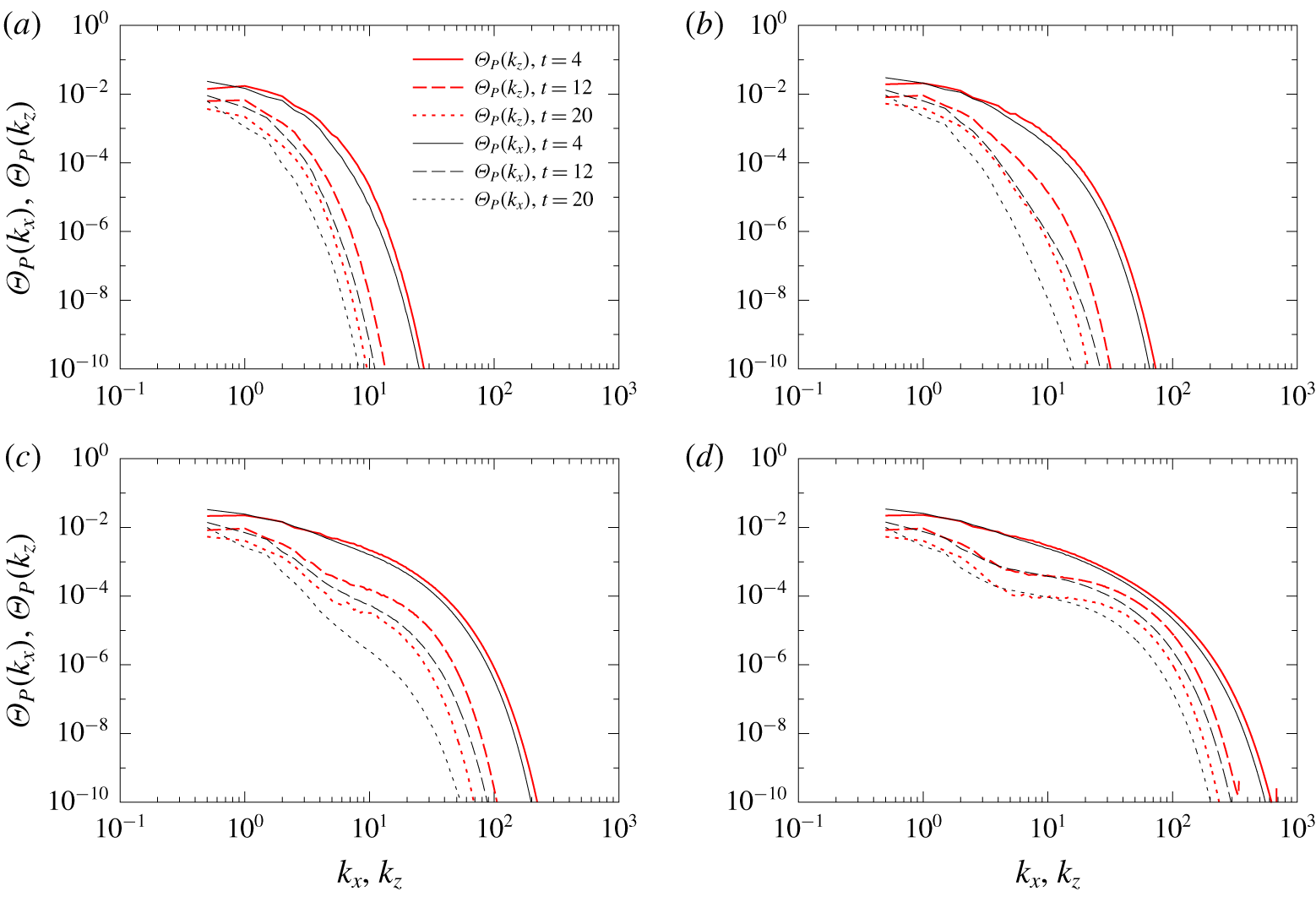
Time development of the one-dimensional spectra of potential energy, i.e.  $\unicode[STIX]{x1D6E9}_{P}(k_{x})$ and
 $\unicode[STIX]{x1D6E9}_{P}(k_{z})$, for (a)
 $Sc=1$, (b)
 $Sc=7$, (c)
 $Sc=70$ and (d)
 $Sc=700$.

The one-dimensional spectra of potential energy are shown in figure 10 to examine the anisotropy of turbulence. The horizontal spectrum  $\unicode[STIX]{x1D6E9}_{P}(k_{x})$ has been measured in most of the experiments (e.g. Lienhard & Van Atta Reference Lienhard and Van Atta1990), and the vertical spectrum
 $\unicode[STIX]{x1D6E9}_{P}(k_{z})$ has sometimes been measured (Keller & Van Atta Reference Keller and Van Atta2000), and these would be preferable for comparison with the experiments. They are computed in this study by
 $$\begin{eqnarray}\unicode[STIX]{x1D6E9}_{P}(k_{x})=\mathop{\sum }_{k_{y},k_{z}}\frac{1}{2Fr_{0}^{2}}(|\hat{\unicode[STIX]{x1D70C}^{\prime }}(k_{x},k_{y},k_{z})|^{2}+|\hat{\unicode[STIX]{x1D70C}^{\prime }}(-k_{x},k_{y},k_{z})|^{2})\frac{1}{k_{min}}\end{eqnarray}$$
and
 $$\begin{eqnarray}\unicode[STIX]{x1D6E9}_{P}(k_{z})=\mathop{\sum }_{k_{x},k_{y}}\frac{1}{2Fr_{0}^{2}}(|\hat{\unicode[STIX]{x1D70C}^{\prime }}(k_{x},k_{y},k_{z})|^{2}+|\hat{\unicode[STIX]{x1D70C}^{\prime }}(k_{x},k_{y},-k_{z})|^{2})\frac{1}{k_{min}}.\end{eqnarray}$$
For all the Schmidt numbers, we note that  $\unicode[STIX]{x1D6E9}_{P}(k_{z})>\unicode[STIX]{x1D6E9}_{P}(k_{x})$ when
 $k_{x}=k_{z}$ except for the lowest wavenumbers (
 $k_{x},k_{z}\sim 1$), showing that the density fluctuations have a vertically thin structure. The weak anisotropy exists already at
 $t=4$, and the anisotropy becomes more significant with time as the Ozmidov scale becomes smaller, and the difference between
 $\unicode[STIX]{x1D6E9}_{P}(k_{x})$ and
 $\unicode[STIX]{x1D6E9}_{P}(k_{z})$ increases. This corresponds to the appearance of small-scale flat structures of density perturbations (figure 2e,f) or the flow dominated by the vertical shear at small scales (Okino & Hanazaki Reference Okino and Hanazaki2019). In a wind tunnel experiment for stratified shear flow, Keller & Van Atta (Reference Keller and Van Atta2000) have compared the horizontal and the vertical spectrum and found that the vertical spectrum is larger than the horizontal spectrum at small scales.
Comparison with the radial spectra  $E_{P}(k)$ in figures 4(a) and 5(a,c,e) shows that the vertical spectra are very similar to the radial spectra (i.e.
 $\unicode[STIX]{x1D6E9}_{P}(k_{z})\simeq E_{P}(k)$ for
 $k_{z}=k$), while the horizontal spectra are generally smaller, especially at small scales (i.e.
 $\unicode[STIX]{x1D6E9}_{P}(k_{x})<E_{P}(k)$ for
 $k_{x}=k$).
The Schmidt number does not affect the anisotropy significantly, but the one-dimensional spectra ( $\unicode[STIX]{x1D6E9}_{P}(k_{x})$,
 $\unicode[STIX]{x1D6E9}_{P}(k_{z})$) and the radial spectra
 $E_{P}(k)$ all extend to the Batchelor wavenumber
 $k_{B}$, with a noticeable flat spectrum only when
 $Sc=700$.
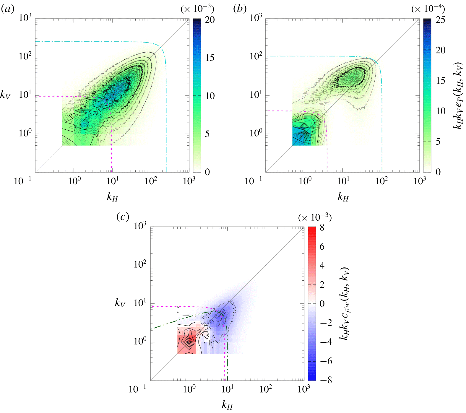
Premultiplied two-dimensional spectra of potential energy  $k_{H}k_{V}e_{P}(k_{H},k_{V})$ for
 $Sc=700$ at (a)
 $t=4$ and (b)
 $t=20$, where contour values are
 $n\times 10^{-3}$ (
 $n=1,2,\ldots$) in (a), and
 $n\times 10^{-4}$ (
 $n=1,2,\ldots$) in (b). Figure 11(c) is the premultiplied two-dimensional cospectrum of vertical density flux
 $k_{H}k_{V}c_{\unicode[STIX]{x1D70C}^{\prime }w}(k_{H},k_{V})$ for
 $Sc=700$ at
 $t=5$, with contour values of
 $2n\times 10^{-3}$ (
 $n=0,\pm 1,\pm 2,\ldots$). The positive and null values are indicated by solid lines, while negative values are indicated by dotted lines. Dashed lines indicate
 $(k_{H}^{2}+k_{V}^{2})^{1/2}=k_{K}$, dashed-dotted lines indicate
 $(k_{H}^{2}+k_{V}^{2})^{1/2}=k_{B}$, and dashed two-dotted line indicates
 $\unicode[STIX]{x1D6FC}=0$, where
 $\unicode[STIX]{x1D6FC}$ is defined by (3.12) in dimensional form.

To further elucidate the anisotropy of potential energy, we consider the two-dimensional spectrum of potential energy and vertical density flux. For example, the two-dimensional spectrum of potential energy  $e_{P}(k_{H},k_{V})$ satisfies
 $$\begin{eqnarray}PE=\int _{0}^{\infty }\text{d}k_{H}\int _{0}^{\infty }\text{d}k_{V}\,e_{P}(k_{H},k_{V}),\end{eqnarray}$$
and is defined by
 $$\begin{eqnarray}e_{P}(k_{H},k_{V})=\frac{k_{H}}{2Fr_{0}^{2}}\int _{0}^{2\unicode[STIX]{x03C0}}\text{d}\unicode[STIX]{x1D719}\,(|\hat{\unicode[STIX]{x1D70C}^{\prime }}(k_{H},\unicode[STIX]{x1D719},k_{V})|^{2}+|\hat{\unicode[STIX]{x1D70C}^{\prime }}(k_{H},\unicode[STIX]{x1D719},-k_{V})|^{2}),\end{eqnarray}$$
where wavevectors are represented in cylindrical coordinates  $\boldsymbol{k}=(k_{H},\unicode[STIX]{x1D719},k_{z})$, with
 $k_{z}$ being the axial coordinate,
 $\unicode[STIX]{x1D719}$ the azimuthal angle and
 $k_{H}=(k_{x}^{2}+k_{y}^{2})^{1/2}$. The two-dimensional cospectrum of vertical density flux
 $c_{\unicode[STIX]{x1D70C}^{\prime }w}(k_{H},k_{V})$ is defined similarly.
At an early time of  $t=4$, figure 11(a) shows that the premultiplied two-dimensional spectrum of potential energy
 $k_{H}k_{V}e_{P}(k_{H},k_{V})$ is symmetric about the line of
 $k_{H}=k_{V}$, indicating an approximate isotropy at all scales when
 $k_{O}<k_{K}$ still holds and
 $k^{-1}$ spectrum is observed in the viscous-convective subrange (figure 4a).
As time proceeds, anisotropy appears in the spectrum, and later at  $t=20$ (figure 11b), the spectrum has two peaks at
 $(k_{H},k_{V})\sim (1,1)$ and
 $(20,30)$, corresponding to the two peaks at
 $k=(k_{H}^{2}+k_{V}^{2})^{1/2}\simeq 1.4$ and 36 in the radial spectrum (figure 6d). The peak at
 $(20,30)$ is in the viscous-convective subrange and satisfies
 $k_{V}>k_{H}$, consistent with the vertically thin structure at small scales observed in figures 2(e) and 3(c).
The two peaks in figure 11(b) appear since the vertical density flux persistently converts the potential energy into kinetic energy near the primitive wavenumber ( $k_{P}=7.1$). The premultiplied two-dimensional cospectrum between density and vertical velocity, i.e.
 $k_{H}k_{V}c_{\unicode[STIX]{x1D70C}^{\prime }w}(k_{H},k_{V})$ (figure 11c), is indeed negative near the Kolmogorov wavenumber or the wavenumbers satisfying
 $\unicode[STIX]{x1D6FC}=0$, which determines the threshold between the decaying oscillation (
 $\unicode[STIX]{x1D6FC}^{2}>0$) and the monotonic decay (
 $\unicode[STIX]{x1D6FC}^{2}<0$) of linear fluctuations (Hanazaki & Hunt Reference Hanazaki and Hunt1996). We note again that
 $\unicode[STIX]{x1D6FC}=0$ in the limit of
 $\unicode[STIX]{x1D703}\rightarrow \unicode[STIX]{x03C0}/2$ (i.e.
 $k_{V}\rightarrow 0$) leads to
 $k=k_{c}\simeq \sqrt{2}k_{P}=10$. The area of negative
 $k_{H}k_{V}c_{\unicode[STIX]{x1D70C}^{\prime }w}$ is off the diagonal (
 $k_{H}=k_{V}$), and mostly satisfies
 $k_{H}>k_{V}$, indicating the anisotropy of the counter-gradient vertical density flux at small scales.
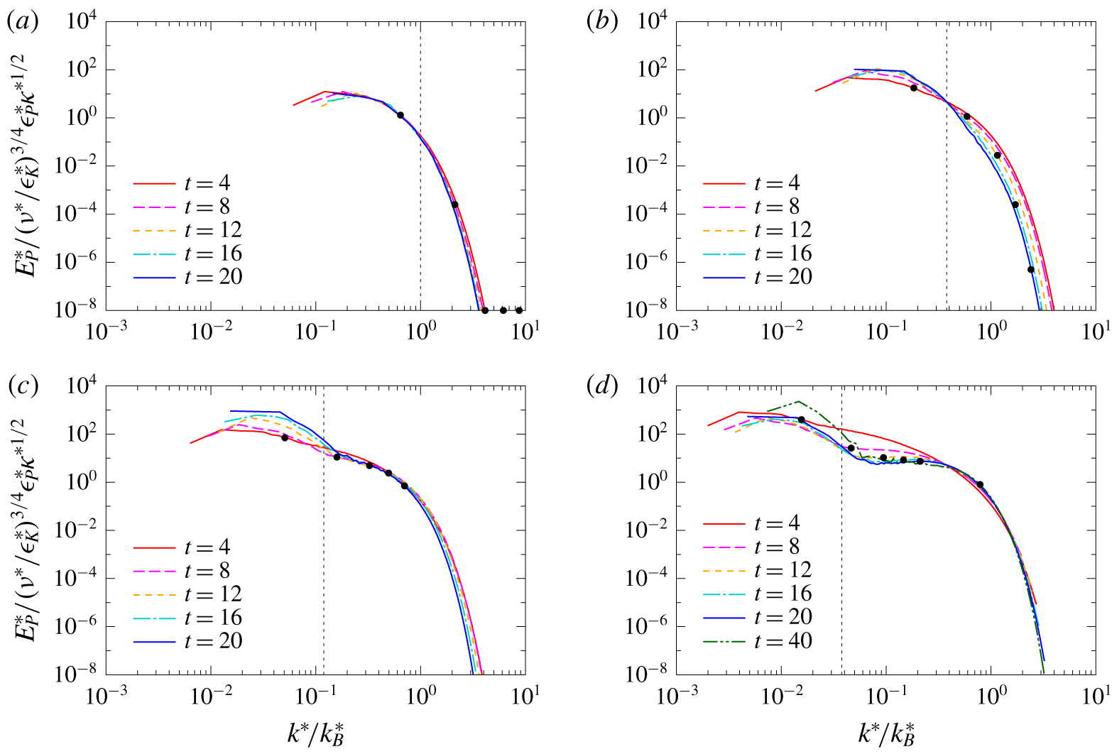
Normalised potential-energy spectrum for (a)  $Sc=1$, (b)
 $Sc=7$, (c)
 $Sc=70$, (d)
 $Sc=700$. The vertical dashed line indicates
 $k_{K}^{\ast }/k_{B}^{\ast }(=Sc^{-1/2})$. Closed circle shows
 $k_{O}^{\ast }/k_{B}^{\ast }$, which increases with time.

Figure 12 shows the time development of the normalised potential-energy spectra. We note that the spectra at different times agree in the decaying process of stratified turbulence. The agreement is incomplete, however, particularly at scales larger than the Ozmidov scale above which the stratification effect is significant. Since the Ozmidov wavenumber increases with time while the Batchelor wavenumber decreases, the normalised wavenumber  $k_{O}^{\ast }/k_{B}^{\ast }$ increases with time. Then, the wavenumber range with unequal normalised spectra extends to higher wavenumbers. On the other hand, since
 $\unicode[STIX]{x1D716}_{K}^{\ast }$ does not change significantly with
 $Sc$,
 $k_{O}^{\ast }/k_{K}^{\ast }=Re_{b}^{-3/4}=(\unicode[STIX]{x1D716}_{K}^{\ast }/(\unicode[STIX]{x1D708}^{\ast }N^{\ast 2}))^{-3/4}$ is rather independent of
 $Sc$. Then,
 $k_{O}^{\ast }/k_{B}^{\ast }(=k_{O}^{\ast }/(k_{K}^{\ast }Sc^{1/2}))$ is smaller for larger
 $Sc$ in general so that the range of unequal spectra becomes narrower for larger
 $Sc$.
4 Conclusions
We have investigated the decaying turbulence in salt-stratified fluid ( $Sc=700$) by direct numerical simulation, with particular attention to the density fluctuations at small scales. As time proceeds and the buoyancy becomes effective below the Kolmogorov scale, the spatial distribution of potential energy begins to show large-scale clouds composed of thin and flat structures smaller than the Kolmogorov scale.
The corresponding potential-energy spectrum shows initially a  $k^{-1}$ spectrum in the viscous-convective subrange in agreement with a passive-scalar spectrum. As time proceeds, however, the spectrum bends and shows a flat spectrum above the bending point. The bending could be attributed to the persistent energy conversion by the counter-gradient flux near the primitive wavenumber
 $k_{P}^{\ast }=\sqrt{N^{\ast }/\unicode[STIX]{x1D708}^{\ast }}$, or rather equivalently, near the Kolmogorov wavenumber.
The results have been tested in this study against different Schmidt numbers ( $Sc=1,7,70$ and
 $700$). However, to investigate the wider applicability of the present results additional simulations with different Reynolds and Froude numbers would be necessary.
Acknowledgements
This study was supported by JSPS KAKENHI grant no. 18K13685, and used computational resources provided by Tohoku University through the HPCI System Research Project (hp180092, hp190091) and by the Earth Simulator Center of the Japan Agency of Marine-Earth Science and Technology.
Declaration of interests
The authors report no conflict of interest.