



1. Introduction
Turbulent flows in ducts and non-circular geometries are common in nature and industrial systems, including rivers, canals and heat exchangers. Therefore, understanding the associated flow physics is essential for accurately predicting species (Wang et al. Reference Wang, Mortimer, Fairweather, Ma and Zhen2024), energy-transfer mechanisms (Modesti & Pirozzoli Reference Modesti and Pirozzoli2022; Karabulut Reference Karabulut2024) and wall shear stresses (Doehring et al. Reference Doehring, Kaller, Schmidt and Adams2024; Santese et al. Reference Santese, Martinez-Sanchis, Sternin and Manfletti2024). A characteristic feature of such flows is the presence of secondary mean velocity components normal to the streamwise direction, typically generated by turbulent stress imbalances and/or duct curvature. For ducts with both circular and non-circular cross-sections, the centrifugal force caused by this curvature induces a secondary mean flow classified as Prandtl’s secondary flow of the first kind. This secondary flow exists in both laminar and turbulent flows, with a secondary mean velocity magnitude of approximately
 $20\,\%$
–
 $30\,\%$
of the streamwise laminar velocity (Demuren & Rodi Reference Demuren and Rodi1984). In contrast, Prandtl’s secondary flows of the second kind, which are the focus of this work, are observed in non-circular straight ducts exhibiting transitional or fully developed turbulence (Prandtl & Tietjens Reference Prandtl and Tietjens1934). The secondary mean velocity magnitude in this flow is about
 $1\,\%$
–
 $3\,\%$
of the streamwise turbulent mean velocity. Despite being small in magnitude, this type of secondary motion plays a major role in the convection of momentum and energy from the mean flow towards the corners. This momentum transport contributes to wall shear stresses near the corners (Modesti et al. Reference Modesti, Pirozzoli, Orlandi and Grasso2018), affecting quantities such as erosion (Winkler et al. Reference Winkler, Rani and Vanka2006) and heat transfer (Wang et al. Reference Wang, Ali, Nadeem, Muhammad and Nofal2021). These secondary flows have been a subject of investigation for more than a century, starting with early experimental visualisations and evolving into detailed numerical studies.
The first documented visualisations of the isotachs (lines of constant velocity magnitude) of the streamwise mean velocity distortions in the corner regions were made by Nikuradse (Reference Nikuradse1926) in experimental investigations of turbulent flow in rectangular and triangular cross-section ducts. Subsequently, Prandtl (Reference Prandtl1927) initiated an effort to understand the secondary flow characteristics and generation mechanisms, proposing that isotach distortions arise from the momentum transport from the main flow towards the corners. Later, Prandtl (Reference Prandtl1952) formulated an explanation based on the surface friction stress balance. His theoretical explanation was confirmed experimentally (Hoagland Reference Hoagland1962) where the surface friction change is consistent with the secondary mean flow direction. Other researchers used turbulent kinetic energy balance (Hinze Reference Hinze1967) to explain the generation and motion of the secondary flows by quantifying the difference between the turbulent kinetic energy and viscous dissipation. However, at that time, it was not yet clear whether secondary flows arise in laminar flows or turbulent flows, nor was the role of Reynolds stresses in their generation fully understood. A subsequent mathematical analysis by Moissis (Reference Moissis1957) demonstrated that secondary flows cannot exist in fully developed laminar flow through a straight duct, while the study by Einstein & Li (Reference Einstein and Li1958) was the first to clearly link secondary flow generation to the vorticity production from Reynolds stresses. Researchers have presented varying perspectives on the role of individual Reynolds production terms in the generation of secondary flows (Brundrett & Baines Reference Brundrett and Baines1964). These differences were generally attributed to the limitations in experimental measurements (Perkins Reference Perkins1970). Further discussion on the streamwise vorticity equation and the secondary flow production will be provided in § 7.
The emergence of direct numerical simulation (DNS) has further improved our understanding of secondary flow dynamics in ducts (Gavrilakis Reference Gavrilakis1992; Huser & Biringen Reference Huser and Biringen1993), enabling the accurate computation of all flow quantities over the entire duct cross-section. For square ducts, simulations have been performed over a wide range of Reynolds numbers in smooth (Zhang et al. Reference Zhang, Trias, Gorobets, Tan and Oliva2015; Modesti et al. Reference Modesti, Pirozzoli, Orlandi and Grasso2018; Pirozzoli et al. Reference Pirozzoli, Modesti, Orlandi and Grasso2018; Modesti & Pirozzoli Reference Modesti and Pirozzoli2022; Xiang et al. Reference Xiang, Su, Hu and Wang2023; Doehring et al. Reference Doehring, Kaller, Schmidt and Adams2024) and ribbed ducts (Santese et al. Reference Santese, Martinez-Sanchis, Sternin and Manfletti2024), enabling the investigation of turbulence statistics and Reynolds number dependence of the secondary flow. Other studies focused on marginally turbulent duct flows at lower Reynolds numbers, where the secondary flow streamlines become increasingly aligned with the mean streamwise vorticity (Pinelli et al. Reference Pinelli, Uhlmann, Sekimoto and Kawahara2010), which in turn emerges due to the preferential emergence of high-speed streaks in the corner region (Uhlmann et al. Reference Uhlmann, Pinelli, Kawahara and Sekimoto2007). It has further been demonstrated by Uhlmann et al. (Reference Uhlmann, Kawahara and Pinelli2010) that the square duct geometry permits travelling wave solutions that result in a secondary mean consistent with that observed in DNS. The duct aspect ratio effect on the secondary flow characteristics has also been numerically (Vinuesa et al. Reference Vinuesa, Noorani, Lozano-Durán, Khoury, Schlatter, Fischer and Nagib2014, Reference Vinuesa, Schlatter and Nagib2015, Reference Vinuesa, Schlatter and Nagib2018) and experimentally (Hoagland Reference Hoagland1962) investigated. Similar to the square duct, in rectangular ducts a pair of counter-rotating vortices exists at each corner, with small and large vortices present along the short and long sides of the duct, respectively. This is in contrast to Prandtl’s original prediction of multiple vortices along the long side of the duct (Prandtl Reference Prandtl1925).
While DNS can accurately capture the characteristics and statistics of turbulent flows in square ducts and other corner geometries, the associated computational cost and scaling with increasing Reynolds number (Choi & Moin Reference Choi and Moin2012) motivates the use and development of closure models capable of capturing features such as the secondary mean. Standard linear eddy viscosity models, based on the Boussinesq relation for the Reynolds stress tensor, have been found to be inadequate for capturing secondary mean flows (Mani et al. Reference Mani, Babcock, Winkler and Spalart2013). More sophisticated Reynolds stress models that solve several transport equations for the components of the Reynolds stress tensor can capture anisotropy of the Reynolds stresses and secondary flow production, though at an increased computational cost. For example, the Speziale–Sarkar–Gatski model (Speziale et al. Reference Speziale, Sarkar and Gatski1991) has demonstrated success in predicting mean quantities in rectangular (De Cacqueray et al. Reference De Cacqueray, Hargreaves and Morvan2009) and trapezoidal (Ansari et al. Reference Ansari, Morvan and Hargreaves2011) duct flows. An alternative and less computationally expensive approach to improve upon linear eddy viscosity models involves their generalisation to nonlinear eddy viscosity formulations, such as the Spalart-quadratic-constitutive relation (QCR) model initially developed by Spalart (Reference Spalart2000). This and several extensions of the QCR framework (Rumsey et al. Reference Rumsey, Carlson, Pulliam and Spalart2020; Sabnis et al. Reference Sabnis, Babinsky, Spalart, Galbraith and Benek2021; Tamaki & Kawai Reference Tamaki and Kawai2024) have been shown to predict the secondary flow in square ducts with accuracy comparable to a Reynolds stress model (Prudenzano et al. Reference Prudenzano, Gand and Deck2025). See (Modesti Reference Modesti2020) for a comprehensive comparison of the performance of different eddy viscosity models in capturing the anisotropic Reynolds stress tensor in square duct flows.
An alternative approach to simplifying the Navier–Stokes equations (NSE) involves the use of restricted nonlinear models based on statistical state dynamics (Farrell & Ioannou Reference Farrell and Ioannou1993; Farrell et al. Reference Farrell, Gayme and Ioannou2017). In this approach, the dynamics of the system are decomposed into those for the streamwise-averaged and fluctuating components, with the nonlinear fluctuation–fluctuation interactions neglected or otherwise modelled. This approach has been applied to predict the presence and features of turbulent flow in a range of configurations, including wall-bounded geometries (Farrell & Ioannou Reference Farrell and Ioannou2012; Farrell et al. Reference Farrell, Ioannou, Jiménez, Constantinou, Lozano-Durán and Nikolaidis2016; Gayme & Minnick Reference Gayme and Minnick2019). It has also been demonstrated that this restricted nonlinear approach can accurately predict mean secondary flow components in turbulent flow over riblets (Zhu et al. Reference Zhu, Viggiano, Minnick and Gayme2025).
The preceding paragraphs have discussed general methods that approximate the solutions to the NSE at reduced computational cost. For a given flow, it is natural to also seek the simplest model capable of reproducing certain pertinent features. For example, various low-dimensional models with sinusoidal basis functions have been proposed to capture the interaction of streamwise streaks and vortices in shear-driven turbulent flows (Waleffe Reference Waleffe1997; Moehlis et al. Reference Moehlis, Faisst and Eckhardt2004; Cavalieri Reference Cavalieri2021). Such reduced-order models (ROMs) are obtained via Galerkin projection, a method whose origins come from Galerkin (Reference Galerkin1915) and are derived from a variational principle belonging to the Rayleigh–Ritz class of problems seeking a simplified system capable of capturing the original system dynamics. The method was originally applied to mechanical systems (Duncan Reference Duncan1937; Batdorf Reference Batdorf1947), then extended to fluid mechanics (Murphy Reference Murphy1973). An advantage of Galerkin projection is that it can be used with any set of linearly independent (ideally orthogonal) basis functions, as long as they span the subspace in which the system attractor is approximately resolved. The introduction of proper orthogonal decomposition (POD) (Lumley Reference Lumley1967; Holmes et al. Reference Holmes, Lumley, Berkooz and Rowley2012) to the fluid mechanics community opened the door for the extensive use of such data-driven empirical basis functions with Galerkin projection across a broad range of flow configurations (Aubry et al. Reference Aubry, Holmes, Lumley and Stone1988; Deane et al. Reference Deane, Kevrekidis, Karniadakis and Orszag1991; Rempfer & Fasel Reference Rempfer and Fasel1994; Moehlis et al. Reference Moehlis, Smith, Holmes and Faisst2002; Rowley et al. Reference Rowley, Mezić, Bagheri, Schlatter and Henningson2009; Schlegel et al. Reference Schlegel, Noack, Comte, Kolomenskiy, Schneider, Farge, Luchtenburg, Scouten and Tadmor2009). The trade-off when using a truncated set of basis functions identified from data is that typically the resulting models are highly tailored to a specific flow configuration and are not robust to parameter variation (Jørgensen et al. Reference Jørgensen, Sørensen and Brøns2003; Noack et al. Reference Noack, Afanasiev, Morzyński, Tadmor and Thiele2003, Reference Noack, Morzyński and Tadmor2011). We are not aware of any prior works seeking Galerkin projection models for modelling turbulent secondary flow in square ducts, though Wedin et al. (Reference Wedin, Biau, Bottaro and Nagata2008) considered a low-dimensional model for self-sustaining processes (SSP) in a square duct geometry, analogous to the work of Waleffe (Reference Waleffe1997) for a wall-bounded shear flow without sidewalls. Proper orthogonal decomposition has also been performed in a square duct geometry for the purposes of identifying the shape and dynamics of coherent structures present in such flows (Matin et al. Reference Matin, Hellström, Hernández-García, Mathiesen and Smits2018; Khan et al. Reference Khan, Anwer, Hasan and Sanghi2020; Lopez-Doriga et al. Reference Lopez-Doriga, Atzori, Vinuesa, Bae, Srivastava and Dawson2024). Since our goal in the present work is to predict properties of turbulent duct flow without any prior data, here rather than using POD modes to obtain a subspace for Galerkin projection, we instead use eigenmodes associated with the underlying linearised dynamics. This choice is motivated in part by the fact that linear mechanisms are known to play an important role in the formation of coherent structures that exist within shear-driven turbulent flows (Lee et al. Reference Lee, Kim and Moin1990; Kim & Lim Reference Kim and Lim2000; Hwang & Cossu Reference Hwang and Cossu2010; McKeon & Sharma Reference McKeon and Sharma2010; Jiménez Reference Jiménez2013).
This work seeks to find the simplest model capable of predicting the existence and qualitative structure of the secondary mean present in turbulent flows through a square duct. The specific approach taken is motivated in part by the findings of the prior work mentioned above. We form Galerkin projection models arising from the interaction of a small number of modes, motivated by the fact that similar low-dimensional models have been found to capture pertinent dynamics in wall-bounded turbulent flows, such as the near-wall cycle (Waleffe Reference Waleffe1997). Furthermore, we focus on streamwise-constant modes, motivated in part by the fact that streamwise-elongated streaks are prevalent in the corner region of turbulent duct flows and are important for the emergence of secondary mean flow (Pinelli et al. Reference Pinelli, Uhlmann, Sekimoto and Kawahara2010; Vinuesa et al. Reference Vinuesa, Prus, Schlatter and Nagib2016; Atzori et al. Reference Atzori, Vinuesa, Lozano-Durán and Schlatter2021). As our objective is to find the simplest ROMs capable of capturing the features of secondary mean flows, additional justification of this streamwise-constant assumption will come from the results obtained, which will demonstrate that streamwise-constant fluctuations are sufficient for this purpose. For our models to yield non-trivial dynamics, we find it necessary to apply an external input to the equations, analogous to the stochastic closure terms used in statistical state dynamics models for turbulent phenomena (Farrell & Ioannou Reference Farrell and Ioannou2012).
The paper is structured as follows. An overview of the governing equations and the geometrical configuration is outlined in § 2. The linearisation of the NSE along with the associated eigenvalue computational approach and symmetry properties are discussed in § 3. In § 4 we describe the Galerkin projection method used to obtain ROMs. Section 5 shows the numerical predictions from running these ROMs, alongside theoretical results obtained directly by analysing their structure. To demonstrate how these ROMs relate to the full system, forced two-dimensional (2D) DNS simulation results are presented in § 6, and ROM predictions of secondary flow production through Reynolds stress quantities are discussed in § 7. Additional discussion and conclusions are provided in § 8.
2. Problem set-up and governing equations
Schematic drawing of the square duct geometry and the associated coordinate system. The duct half-height is
 $h$
and the streamwise flow is in the positive
 $x$
direction, as indicated by the green arrows and curve. While the laminar streamwise flow is plotted as a function of
 $y$
at
 $z=0$
, the full 2D profile is a function of both
 $y$
and
 $z$
(as depicted in figure 2
a).

Figure 1. Long description
A diagram of a square duct geometry and the associated coordinate system. The duct has a half-height denoted by h. The streamwise flow is indicated by green arrows and a curve, moving in the positive direction. The diagram shows the laminar streamwise flow as a function of the y-coordinate at a specific z-coordinate. The full 2D profile of the flow is a function of both the y and z coordinates. The coordinate system includes axes labeled as x-hat, y-hat, and z-hat, representing the streamwise, vertical, and spanwise directions, respectively.
This section describes the duct flow configuration and the basic properties of the corresponding incompressible NSE. Figure 1 shows a schematic drawing of the square duct along with the non-dimensional coordinates
 $x$
,
 $y$
and
 $z$
denoting the streamwise and cross-stream directions, respectively. The associated velocity vector is defined as
 $\hat {\boldsymbol{u}}=u \boldsymbol {i}+v \boldsymbol {j} +w\boldsymbol {k}$
, where
 $\boldsymbol {i},\;\boldsymbol {j}\; \mathrm{and}\; \boldsymbol {k}$
are the Cartesian unit vectors. We choose
 $h,\; \hat {U}_c, \;h/\hat {U}_c\; \mathrm{and}\; \rho \hat {U}_c^2$
as length, velocity, time and pressure scales, respectively, where
 $(\hat {\boldsymbol{\cdot }})$
denotes the dimensional quantities. The velocity
 $\hat {U}_c$
is the centreline laminar velocity and
 $h$
is the duct half-height. The associated non-dimensional NSE and continuity equations are given by
 \begin{align} \partial _t \boldsymbol{u} + \boldsymbol{u} \boldsymbol{\cdot }\boldsymbol{\nabla }\boldsymbol{u} &=-\boldsymbol{\nabla }p +Re^{-1} \;{\nabla} ^2 \boldsymbol{u},\end{align}
 \begin{align} \boldsymbol{\nabla }\boldsymbol{\cdot }\boldsymbol{u} &=0,\end{align}
with no-slip boundary conditions
 \begin{align} \boldsymbol{u}(x,y = \pm 1,z) = \boldsymbol{u}(x,y, z = \pm 1)=0, \end{align}
where the Reynolds number is defined as
 $ \textit{Re}=\hat {U}_c h/\nu$
. We decompose the flow field variables into a base state and time-dependent fluctuations as
 \begin{align} \boldsymbol{u} (\boldsymbol{x},t)&=\boldsymbol{U}(\boldsymbol{x})+ \boldsymbol{u}'(\boldsymbol{x},t),\end{align}
 \begin{align} p (\boldsymbol{x},t)&=P_o+\frac {{\rm d}P(x)}{{\rm d}x}x+\; p'(\boldsymbol{x},t),\end{align}
where
 $\boldsymbol{U}(\boldsymbol{x})=U(y,z)\boldsymbol {i}+0\boldsymbol {j}+0\boldsymbol {k}$
is the base (laminar) velocity profile,
 $\boldsymbol{u}'=u'\boldsymbol {i}+v'\boldsymbol {j}+w'\boldsymbol {k}$
and
 $P_o$
is an integration constant. While we consider a general three-component fluctuating velocity for the purposes of this derivation, the ROMs that we identify will only consider cross-stream (
 $v',w'$
) fluctuations, which themselves will be streamwise constant. Both
 $\boldsymbol{U}$
and
 $\boldsymbol{u}'$
satisfy the same boundary conditions as the total velocity indicated in (2.2). Setting
 $\boldsymbol{u}'=0$
in (2.3) and substituting the resulting decomposition into (2.1) gives the steady laminar base-flow equations
 \begin{align} \boldsymbol{U} \boldsymbol{\cdot }\boldsymbol{\nabla }\boldsymbol{U} &=-\boldsymbol{\nabla }P +Re^{-1} {\nabla} ^2 \boldsymbol{U} ,\end{align}
 \begin{align} \boldsymbol{\nabla }\boldsymbol{\cdot }\boldsymbol{U} &=0.\end{align}
The linearised equations governing the fluctuating components are obtained by subtracting (2.4) from (2.1) while utilising the decomposition (2.3) and neglecting the nonlinear
 $\boldsymbol{u}'\boldsymbol{\cdot }\boldsymbol{\nabla }\boldsymbol{u}'$
term, giving
 \begin{align} \partial _t \boldsymbol{u}' +\boldsymbol{U}\boldsymbol{\cdot }\boldsymbol{\nabla }\boldsymbol{u}' +\boldsymbol{u}' \boldsymbol{\cdot }\boldsymbol{\nabla }\boldsymbol{U} + \boldsymbol{\nabla }p' -Re^{-1} {\nabla} ^2 \boldsymbol{u}' &= 0 ,\end{align}
 \begin{align} \boldsymbol{\nabla }\boldsymbol{\cdot }\boldsymbol{u}'&= 0 .\end{align}
The base laminar solution to (2.4) is obtained by solving the 2-D Poisson equation
 \begin{align} \left (\partial _{yy}+\partial _{zz}\right )U(y,z)=-Re \; \frac {{\rm d} P(x)} {{\rm d} x} =C_1, \end{align}
again with the no-slip boundary conditions
 $U(y,z=\pm 1) = U(y=\pm 1,z)=0$
. Setting
 $C_1=-3.393449$
(Wedin et al. Reference Wedin, Biau, Bottaro and Nagata2008) gives a dimensionless centreline velocity
 $U_c=1$
. The solution of (2.6) can be expressed as a series solution (Panton Reference Panton2024)
 \begin{align} U(y,z)= C_2\big ( 1 -y^2\big )+ C_3 \sum _{n=1}^{\infty } \frac {(-1)^n}{\alpha _n ^2} \cos {(\alpha _n y)} \frac {\cosh {(\alpha _n z)} }{\cosh {(\alpha _n )}}, \end{align}
where
 $\alpha _n=(2n-1)\pi /2$
,
 $C_2 = 1.69672$
and
 $C_3 = 6.78689$
. Figure 2(a) shows contours of this 2D laminar flow (which is independent of Reynolds number), compared with a turbulent mean flow (figure 2
b) from DNS simulations (Vinuesa et al. Reference Vinuesa, Noorani, Lozano-Durán, Khoury, Schlatter, Fischer and Nagib2014) at a Reynolds number
 $ \textit{Re} = 2796$
(based on the centreline velocity). As shown, the streamwise velocity is flattened across the duct cross-section towards the walls and deformed near the corner due to the secondary flow.
(a) Laminar and (b) turbulent mean flow from DNS simulations at
 $ \textit{Re}=2796$
(Vinuesa et al. Reference Vinuesa, Noorani, Lozano-Durán, Khoury, Schlatter, Fischer and Nagib2014). The coloured contours show the streamwise velocity distribution and the vectors show the secondary turbulent mean velocity. Both contour plots are normalised by the corresponding maximum streamwise velocity.

3. Basis function computation and properties
Using Galerkin projection models requires the selection of basis functions upon which we project the governing equations. Here, we describe how these basis functions are chosen and selected. Since we do not assume any prior knowledge of the turbulent flow field, we cannot use POD modes as often when identifying low-dimensional models via Galerkin projection. Instead, we choose to use eigenmodes of the linearised NSE for this system as basis functions. We describe these linearised equations for the square duct in § 3.1, before discussing the numerical methods by which these eigenmodes are computed in § 3.2. The properties of these eigenmodes, particularly the geometrical symmetries that they can possess, are discussed in § 3.3.
3.1. Linearised equations and their eigendecomposition
The eigenvalue problem of the linearised system (2.5) around a streamwise laminar base flow is obtained by assuming a fully developed flow that is homogeneous in the streamwise direction. In particular, we consider a fluctuating velocity field of the form
 \begin{align} \boldsymbol{u}'(\boldsymbol{x},t)=\tilde {\boldsymbol{u}}(k_x,\lambda ;y,z)\;\exp {(\text{i} k_x x+\lambda t)}, \end{align}
where
 $\lambda$
determines the temporal evolution of this fluctuation and
 $k_x$
is the streamwise wavenumber. Note that while
 $\lambda$
is generally complex (and indeed is often expressed in terms of a complex frequency), it is real for the streamwise-constant eigenproblems considered in the present work. Substituting (3.1) into (2.5), we get a linearised eigensystem decomposition of the form
 \begin{align} \lambda \tilde {\boldsymbol{u}} =-\boldsymbol{U} \boldsymbol{\cdot }\tilde {\boldsymbol{\nabla }} \tilde {\boldsymbol{u}} -\tilde {\boldsymbol{u}} \boldsymbol{\cdot }\tilde {\boldsymbol{\nabla }} \boldsymbol{U} -\tilde {\boldsymbol{\nabla }} \tilde {p} +Re^{-1} \tilde {{\nabla} }^2 \tilde {\boldsymbol{u}},\quad \tilde {\boldsymbol{\nabla }} \boldsymbol{\cdot }\tilde {\boldsymbol{u}}=0, \end{align}
where the transformed gradient operator is
 $\tilde {\boldsymbol{\nabla }}:= \text{i}k_x\boldsymbol {i}+\partial _y\boldsymbol {j}+\partial _z\boldsymbol {k}$
and the Laplacian operator is
 $\tilde {{\nabla} }^2:=-k_x^2+\partial _y^2+\partial _z^2$
. Equation (3.2) can be expressed in a matrix form as
 \begin{align} { \left [\lambda {\unicode{x1D63D}} \ + \ \begin{pmatrix} {\unicode{x1D647}}_{1} & \partial _yU & \partial _z U & {\text{i}}k_x \\[5pt] 0 & {\unicode{x1D647}}_{1} & 0 & \partial _y \\[5pt] 0 & 0 & {\unicode{x1D647}}_{1} & \partial _z \\[5pt] {\text{i}}k_x & \partial _y & \partial _z & 0 \end{pmatrix}\right ] \begin{pmatrix} \boldsymbol \phi ^{u} \\[5pt] \boldsymbol \phi ^{v} \\[5pt] \boldsymbol \phi ^{w} \\[5pt] \boldsymbol \phi ^{p} \end{pmatrix} }=(\lambda {\unicode{x1D63D}} +{\unicode{x1D63C}}) \begin{pmatrix} \boldsymbol \phi ^{(u,v,w)} \\[5pt] \boldsymbol \phi ^{p} \end{pmatrix} =0, \end{align}
where
 \begin{align} {\unicode{x1D647}}_{1} = \text{i} k_xU -Re^{-1}\tilde {{\nabla} }^2 \end{align}
and
 \begin{align} {\unicode{x1D63D}}= \begin{pmatrix} 1& 0 & 0 & 0 \\[5pt] 0 & 1 & 0 & 0 \\[5pt] 0 & 0& 1 & 0 \\[5pt] 0 & 0 & 0 & 0 \\[5pt] \end{pmatrix} \! . \end{align}
The
 $\boldsymbol \phi ^{u},\boldsymbol \phi ^{v}$
and
 $\boldsymbol \phi ^{w}$
correspond to the streamwise and cross-stream components of the eigenmode
 $\boldsymbol \phi$
, respectively, and the superscript
 $(\boldsymbol{\cdot })^{(u,v,w)}$
is read as an eigenvector
 $\boldsymbol \phi$
with
 $u,v$
and
 $w$
components. Here and throughout, (3.3a
) is completed by the Dirichlet boundary conditions
 $\boldsymbol \phi ^{(u,v,w)}(y = \pm 1,z) = \boldsymbol \phi ^{(u,v,w)}(y,z = \pm 1) = 0$
. The differential operator of (3.3a
) is non-normal; that is,
 $({\unicode{x1D63C}}{\unicode{x1D63C}}^* \neq {\unicode{x1D63C}}^*{\unicode{x1D63C}})$
, where
 ${\unicode{x1D63C}}^*$
is the adjoint operator. Therefore, its eigenmodes are not orthogonal.
From this point on, we only consider streamwise-constant fluctuations, where
 $k_x = 0$
in (3.2). In this case, (3.3) simplifies to
 \begin{align} { \left [\lambda {\unicode{x1D63D}}\ + \ \begin{pmatrix} {\unicode{x1D647}}_{2} & \partial _yU & \partial _z U & 0 \\[5pt] 0 & {\unicode{x1D647}}_{2} & 0 & \partial _y \\[5pt] 0 & 0 & {\unicode{x1D647}}_{2} & \partial _z \\[5pt] 0 & \partial _y & \partial _z & 0 \end{pmatrix}\right ] \begin{pmatrix} \boldsymbol \phi ^{u} \\[5pt] \boldsymbol \phi ^{v} \\[5pt] \boldsymbol \phi ^{w} \\[5pt] \boldsymbol \phi ^{p} \end{pmatrix}=0 }, \end{align}
where
 ${\unicode{x1D647}}_{2} = -Re^{-1}(\partial _{yy}+\partial _{zz})$
. In this case, non-normality arises due to the off-diagonal terms,
 $\partial _yU$
and
 $\partial _zU$
. For this streamwise-constant case, the operator is block upper triangular and can be recast in a compact form as
 \begin{align} \begin{pmatrix} A_u & C_{(v,w) \rightarrow u}\\[5pt] 0 & A_{v,w,p} \end{pmatrix} \begin{pmatrix} \boldsymbol \phi ^{u}\\[5pt] \boldsymbol \phi ^{v,w,p} \end{pmatrix}=0, \end{align}
where
 $A_u = \lambda + {\unicode{x1D647}}_{2}$
is the top-left block,
 $A_{v,w,p}$
is the lower-right
 $3\times 3$
block and
 $C_{(v,w) \rightarrow u} = \begin{pmatrix}\partial _yU & \partial _z U & 0 \end{pmatrix}$
is the upper off-diagonal block of (3.4). The non-normality of the full operator arises from this off-diagonal block that maps from transverse velocity components to the streamwise velocity component. Because the operator is block upper triangular, its generalised eigenvalues are the values of
 $\lambda$
for which either diagonal block is singular, yielding the two separate eigenvalue problems given by
 \begin{align} \left [\lambda ^{u} \ + \ {\unicode{x1D647}}_2\right ]\boldsymbol \phi ^u_{{Laplace}} = 0, \\[-28pt] \nonumber \end{align}
 \begin{align} \left [\lambda ^{(v,w)}\begin{pmatrix} 1 & 0 & 0\\[5pt] 0 &1 & 0\\[5pt] 0 & 0 & 0 \end{pmatrix}\ + \ \begin{pmatrix} {\unicode{x1D647}}_{2} & 0 & \partial _y \\[5pt] 0 & {\unicode{x1D647}}_{2} & \partial _z \\[5pt] \partial _y & \partial _z & 0 \end{pmatrix}\right ] \begin{pmatrix} \boldsymbol \phi ^{v} \\[5pt] \boldsymbol \phi ^{w} \\[5pt] \boldsymbol \phi ^{p} \end{pmatrix}= 0, \\[0pt] \nonumber \end{align}
where
 $\lambda ^u$
and
 $\lambda ^{(v,w)}$
are the eigenvalues associated with the streamwise eigenproblem and cross-stream eigenproblem, respectively. Equation (3.6a
), corresponding to eigenmodes with only a streamwise component, is equivalent to an eigenproblem of the Laplace operator, with solutions given by
 \begin{align} \boldsymbol \phi ^u_{{Laplace},(j,k)}= \sin \left ( \frac {j\pi }{2} (y+1)\right )\sin \left (\frac {k \pi }{2} (z+1)\right ) \!, \\[-28pt] \nonumber \end{align}
 \begin{align} \lambda ^{u}_{(j,k)} = -\frac {\pi ^2}{4Re}\big ( j^2+k^2\big ), \\[0pt] \nonumber \end{align}
where the modal indices
 $j,k=1,2,3,\ldots$
and the eigenmodes
 $\boldsymbol \phi ^u_{{Laplace}}$
are orthonormal.
The generalised eigenproblem given in (3.6b
) corresponds to the 2D Stokes operator. The eigenvalues and eigenmodes for this operator must be computed numerically, which will be discussed in the next section. While the eigenvalues
 $\lambda ^{(v,w)}$
only depend on the lower diagonal block of (3.4), the corresponding eigenmodes will also have a streamwise component, owing to the off-diagonal block
 $C$
. The streamwise component of these eigenmodes is given by
 \begin{align} \big [\lambda ^{(v,w)} + {\unicode{x1D647}}_2\big ]\boldsymbol \phi ^u_{{response}}=- \left (\partial _yU\; \boldsymbol \phi ^v+\partial _zU\;\boldsymbol \phi ^w\right ), \quad \text{for all } \lambda ^{(v,w)} \;\notin \sigma ({\unicode{x1D647}}_2) ,\end{align}
where
 $\sigma ({\unicode{x1D647}}_2)$
is the spectrum of the operator
 ${\unicode{x1D647}}_2$
. The equation shows that the cross-stream velocity components of the lower-block eigenmodes on the right-hand side of the equation act as a forcing, triggering a response in the streamwise direction.
From the previous discussion, for the case
 $k_x=0$
, we note that while the operators in (3.6a
)–(3.6b
) are Hermitian and, thus, have orthogonal eigenmodes, the eigenmodes of the full operator (3.4) are not orthogonal, owing to the streamwise component of the lower-block eigenmodes given in (3.8). The eigenmode of the lower diagonal block,
 $A_{v,w,p}$
, corresponds to the Stokes eigenmodes (3.6b
) and is self-adjoint with a real spectrum; therefore, the corresponding eigenmodes form a complete orthonormal basis in the space of divergence-free cross-stream velocity fields. Since the present work focuses on modelling the secondary velocity components, the ROMs are constructed using the eigenmodes of this cross-stream Stokes problem, rather than the full non-orthogonal eigenmodes of (3.4). Therefore, the basis functions of the ROMs contain only the secondary velocity components and are written as
 $\boldsymbol \phi ^{(v,w)} (y,z)= ( \boldsymbol \phi ^v (y,z), \boldsymbol \phi ^w (y,z) )^T$
. The superscript
 $(\boldsymbol{\cdot })^{(v,w)}$
will be dropped in the following sections for simplicity. The computation and structure of these eigenfunctions will be discussed in §§ 3.2 and 3.3, respectively.
We further note that while the eigenvalues of (3.6a
) and (3.6b
) depend on the Reynolds number, the eigenmodes, and thus, the subspace used to define our ROMs, will be independent of the Reynolds number. We could eliminate this Reynolds number dependency altogether by redefining the velocity scale to be
 $\hat {U}_c=\nu /h$
, which would replace
 $ \textit{Re}$
by unity in (3.4)–(3.8).
There are several advantages to using this choice of eigenmodes over others that could be formulated, such as those obtained from resolvent or transient growth analysis, or through balanced POD. The current eigenmode formulation allows for the secondary velocity components to be entirely decoupled from the streamwise components while still yielding orthonormal modes, whereas when applied to the full three-component system, the other methods mentioned generally give modes with coupled velocity components. In practice, this can lead to models that make it difficult to isolate the secondary flow dynamics, since the leading modes are often dominated by streamwise velocity components. Additionally, within the present streamwise-constant formulation, the cross-stream basis functions are independent of the choice of laminar or turbulent streamwise base/mean velocity profile. This is advantageous if the mean is not known in advance, and also for showing that the predictions of the ROMs are not sensitive to this choice of linearisation point.
3.2. Computation of eigenmodes
We now discuss the approach to numerically compute the eigenvalues and eigenmodes of the Stokes operator described in (3.6b
). Considerable effort has been directed towards developing efficient numerical solvers for the Stokes operator across both 2D and three-dimensional geometries, including square (Leriche & Labrosse Reference Leriche and Labrosse2004), triangular (Chen et al. Reference Chen, Labrosse, Lallemand and Luo2016) and cubic domains (Labrosse et al. Reference Labrosse, Leriche and Lallemand2014). The choice of solution methodology for the Stokes problem depends on the selected variables, whether primitive flow variables (Arrow et al. Reference Arrow, Hurwicz, Uzawa, Chenery, Johnson and Karlin1958; Chorin Reference Chorin1968; Kleiser & Schumann Reference Kleiser and Schumann1980) or streamfunction formulations (Batoul et al. Reference Batoul, Khallouf and Labrosse1994; Leriche & Labrosse Reference Leriche and Labrosse2004). A common objective of these Stokes solvers is the decoupling between the pressure and velocity fields. However, with modern computational capabilities, direct solutions to large-scale eigenvalue problems are feasible without iterative or splitting schemes. Therefore, we solve the eigenvalue problem of the linear differential operator using the MATLAB function eigs that utilises the implicitly restarted Arnoldi method in the ARPACK library (Lehoucq et al. Reference Lehoucq, Sorensen and Yang1998). Spatial discretisation is carried out using the Chebyshev collocation spectral method, with an equal number of Chebyshev nodes, denoted as
 $N_c=96$
, in each spatial direction. The no-slip boundary condition is implicitly imposed on the velocity field using the methods described in Trefethen (Reference Trefethen2000), restricting computations to the internal nodes of the domain.
3.3. Eigenmode structure and symmetries
Vector field plots of the twelve least stable eigenmodes
 $\boldsymbol \phi$
of (3.6b
), arranged from least to most stable. A total of 96 Chebyshev nodes are used in both the
 $y$
and
 $z$
directions.

Figure 3. Long description
The image contains twelve vector field plots arranged in a 3x4 grid. Each plot represents the least stable eigenmodes of equation (3.6b), ordered from least to most stable. The plots are labeled from (1) to (12). Each plot has axes labeled ‘y’ and ‘z’, ranging from -1 to 1. The vector fields depict various patterns of flow distortions, with arrows indicating the direction and magnitude of the velocity vectors. Panel (1) shows a circular pattern, Panel (2) displays a spiral pattern, Panel (3) exhibits a distorted square pattern, and Panel (4) shows a more complex pattern with multiple vortices. Panel (5) presents a pattern with four distinct vortices, Panel (6) shows a spiral pattern similar to Panel (2), Panel (7) exhibits a pattern with eight vortices, and Panel (8) displays a complex pattern with multiple vortices. Panel (9) shows horizontal lines, Panel (10) displays vertical lines, Panel (11) exhibits a pattern with multiple vortices, and Panel (12) shows a complex pattern with multiple vortices.


The twelve least stable eigenmodes of (3.6b
) are shown in figure 3, arranged in increasing order of stability (damping rate). All eigenmodes exhibit vortical structures, which are largest for the least stable modes. The structure of these modes is consistent with the eigenmodes of the Stokes operator reported in Leriche & Labrosse (Reference Leriche and Labrosse2004). The spectrum of these eigenmodes is shown in figure 4 scaled by the Reynolds number,
 $ \textit{Re}$
. We find that all eigenvalues are stable and observe that there are several repeated eigenvalues, which arise due to the symmetries present in the square duct geometry. While these cross-stream basis modes are asymptotically stable, the transient secondary flows that they are associated with are a key component of linear amplification mechanisms that can yield large growth, owing to the non-normality of the linear operator. Galletti & Bottaro (Reference Galletti and Bottaro2004) showed that in square ducts, optimally configured cross-stream vortices induce large transient amplification despite being asymptotically stable. They found that, for a turbulent mean profile, large-scale secondary structures can be sustained over long streamwise distances through a linear transient mechanism.
Subsets of these eigenmodes will be used as basis functions for identifying ROMs. The properties and predictions of these ROMs will be dependent on the properties of the eigenmodes used, with the symmetries of the chosen eigenmodes being particularly important for obtaining mean field predictions with expected symmetries. These eigenmodes are 2D vector fields defined on a square domain, which can feature two fundamental planar isometries: rotational symmetry (
 $\theta $
rotation) and reflectional symmetry (
 $\beta $
reflection) (Leriche & Labrosse Reference Leriche and Labrosse2004). These symmetries play an important role in shaping the structure of eigenmodes and the subsequent flow field predicted by ROMs. Given a 2D eigenmode
 $\boldsymbol \phi (y,z)= ( \boldsymbol \phi ^v (y,z), \boldsymbol \phi ^w (y,z) )^T$
, its rotational symmetry is expressed as
 \begin{align} \boldsymbol{\phi }'(y',z')=\mathcal{R}(\theta )\boldsymbol \phi \left (\mathcal{R}(\theta )(y,z)\right ), \end{align}
where
 $\mathcal{R}(\theta )$
is a rotational transformation matrix defining a coordinate transformation of the form
 \begin{align} \begin{pmatrix} y' \\[3pt] z' \\[3pt] \end{pmatrix}= \begin{pmatrix} \cos {\theta } & \sin {\theta } \\[3pt] -\sin {\theta }& \cos {\theta } \end{pmatrix} \begin{pmatrix} y \\[3pt] z \\[3pt] \end{pmatrix} \!. \end{align}
Similarly, a reflection transformation about an angle
 $\beta$
is accomplished using the reflection transformation matrix
 $\mathcal{L}(\beta )$
, defined as
 \begin{align} \boldsymbol{\phi }''(y'',z'')=\mathcal{L}(\beta ) \boldsymbol \phi \left ( \mathcal{L}(\beta ) (y,z) \right ) ,\end{align}
with the coordinate reflection expressed as
 \begin{align} \begin{pmatrix} y'' \\[3pt] z'' \\ \end{pmatrix}= \begin{pmatrix} -\cos {\beta } & \sin {\beta } \\[3pt] \sin {\beta }& \cos {\beta } \end{pmatrix} \begin{pmatrix} y \\[3pt] z \\ \end{pmatrix} \!. \end{align}
The
 $\theta$
and
 $\beta$
angles denote an anticlockwise rotation by an angle
 $\theta$
and a reflection around a line with an angle
 $\beta /2$
with the positive
 $z$
axis, respectively. Note that the transformation matrices
 $\mathcal{R}$
and
 $\mathcal{L}$
are written such that the first row corresponds to the transformation of the vertical coordinate
 $y$
and the second row corresponds to the horizontal coordinate
 $z$
. The square has four rotational and four reflection symmetries characterised by angles
 $\theta$
and
 $\beta$
as multiples of
 $\pi /2$
and summarised in table 1.
Symmetry transformations of the cross-stream eigenmode vector field
 $\boldsymbol \phi (y,z)=( \boldsymbol \phi ^v,\boldsymbol \phi ^w )^T$
under
 $\mathcal{R}(\theta )$
(rotations) and
 $\mathcal{L}(\beta )$
(reflections), with the corresponding coordinate mappings.

Table 1. Long description
Panel A: A table listing angles and their corresponding transformed fields and coordinate mappings. The angles include theta, pi over 2, pi, negative pi over 2, 2 pi, beta over 2, pi over 4, pi over 2, 3 pi over 4, and pi. Each angle has a specific transformed field equation and coordinate mapping. Panel B: Detailed equations for transformed fields and coordinate mappings for each angle. The transformed fields involve vectors and matrices, while the coordinate mappings involve coordinate transformations.
Of the eigenmodes shown in figure 3, only mode 12 satisfies all eight possible geometric symmetries. This will be important when it comes to selecting modes to use for a ROM, since the inclusion of such a fully symmetric mode will be required for the prediction of secondary mean flow that also satisfies all symmetries. Note that while mode 12 is the only such fully symmetric mode shown in figure 3, it is one of a family of such eigenmodes of the square duct geometry, with all others being even more stable.
We finally note that we are not the first to observe the similarity between the secondary flow and eigenmodes of linear operators in the square duct geometry. Pirozzoli et al. (Reference Pirozzoli, Modesti, Orlandi and Grasso2018) found that the Helmholtz equation associated with the secondary flow streamfunction under an inviscid assumption admits solutions (corresponding to eigenmodes of the Laplacian) that resemble the secondary mean. In addition, Wedin et al. (Reference Wedin, Biau, Bottaro and Nagata2008) used Stokes eigenmodes (equivalent to those shown in figure 3) to represent streamwise-constant rolls in their model for SSP, though they found that a four-vortex mode (equivalent to mode 4 in figure 3) was more conducive to self-sustaining dynamics than the eight-vortex configuration.
4. Galerkin projection
In this section we discuss the Galerkin projection method for approximating the incompressible NSE and the derivation of the evolution equations for internal flow with Dirichlet boundary conditions. Assuming a streamwise-constant flow and neglecting streamwise fluctuations, we approximate the cross-stream dynamics as
 \begin{align} \boldsymbol{u} (y,z,t) = \begin{pmatrix} U(y,z)\\[4pt] 0\\[4pt] 0 \end{pmatrix}+ \begin{pmatrix} 0\\[4pt] v'(y,z,t)\\[4pt] w'(y,z,t) \end{pmatrix} \approx \begin{pmatrix} U(y,z)\\[4pt] 0\\[4pt] 0 \end{pmatrix} +\sum _{i=1}^{N} a_i(t) \boldsymbol \phi _i(y,z), \\[-28pt] \nonumber \end{align}
 \begin{align} \frac {\text{d} \boldsymbol{a}}{\text{d} t}=\boldsymbol{F}(\boldsymbol{a}), \\[0pt] \nonumber \end{align}
where
 $\boldsymbol{a}=(a_1,a_2,a_3, {\cdots} ,a_N)^T$
and
 $\boldsymbol \phi _i=(0,\boldsymbol \phi ^v_i,\boldsymbol \phi ^w_i)^T$
. In this formulation, the total velocity field
 $\boldsymbol{u}$
is approximated as a laminar velocity profile,
 $U(y,z),$
and a summation of spatial basis functions
 $\boldsymbol \phi _i(y,z)$
multiplied by time-evolving magnitudes
 $a_i(t)$
known as expansion coefficients. The expansion coefficients are governed by a system of ordinary differential equations (ODEs)
 $\boldsymbol{F}(\boldsymbol{a})$
. Equation (4.1) is therefore a low-order
 $N$
-dimensional representation of the cross-stream dynamics of the streamwise-constant NSE.
The system of ODEs for the expansion coefficients (4.1b ) is derived by solving an optimisation problem that involves the projection of the basis functions onto the residual of the Galerkin expansion of the NSE within the same subspace (Cassel Reference Cassel2013). The residual of the NSE is expressed as
 \begin{align} \mathscr{R}(\boldsymbol{u})=\partial _t \boldsymbol{u} + \boldsymbol{u} \boldsymbol{\cdot }\boldsymbol{\nabla }\boldsymbol{u} +\boldsymbol{\nabla }p -Re^{-1} \;{\nabla} ^2 \boldsymbol{u} ,\end{align}
and the projection would be in the form
 \begin{align} \left \langle \boldsymbol{\phi }_i, \mathscr{R}\left ( \sum _{j=0}^{N}a_{\kern-1pt j}(t)\boldsymbol{\phi }_{\kern-1pt j}(y,z) \right ) \right \rangle _{\varUpsilon }=0, \quad i=1,\ldots ,N, \end{align}
where
 $\langle \boldsymbol{\cdot }, \boldsymbol{\cdot }\rangle _\varUpsilon$
is the standard inner product on the domain
 $\varUpsilon$
and, for simplicity, we let
 $\boldsymbol{\phi _0}=\boldsymbol{U}(y,z)$
and
 $a_0=1$
. Assuming orthonormal basis functions, the resulting quadratically nonlinear system of ODEs can be expressed as
 \begin{align} \dfrac {\text{d}a_i}{\text{d}t}=-\sum _{j=0}^N \sum _{k=0}^N a_{\kern-1pt j} a_k\; \langle \boldsymbol \phi _{\kern-1pt j} \boldsymbol{\cdot }\boldsymbol{\nabla }\boldsymbol \phi _k , \boldsymbol \phi _i \rangle +Re^{-1} \sum _{j=0}^N a_{\kern-1pt j} \; \langle {\nabla} ^2 \boldsymbol \phi _{\kern-1pt j},\boldsymbol \phi _i \rangle , \quad i=1,\ldots ,N, \end{align}
where the inner product
 $\langle {\nabla} ^2 \boldsymbol \phi _{\kern-1pt j},\boldsymbol \phi _i \rangle$
is the projection of the viscous term,
 $\langle \boldsymbol \phi _{\kern-1pt j} \boldsymbol{\cdot }\boldsymbol{\nabla }\boldsymbol \phi _k , \boldsymbol \phi _i \rangle$
is the nonlinear advection term. The projection of the pressure gradient vanishes identically for internal incompressible flow with Dirichlet and periodic boundary conditions (Holmes et al. Reference Holmes, Lumley, Berkooz and Rowley2012), which can be shown by transforming the volume into a surface integral using the divergence theorem. It should be noted that the pressure gradient has no impact on the Galerkin projection of this type of flow field, but for open flows, this term can be crucial and computationally expensive (Noack et al. Reference Noack, Papas and Monkewitz2005). Equation (4.4) can also be generalised to include additional closure terms to account for unmodelled dynamics, which will be utilised in the forthcoming analysis. To achieve spectral accuracy in solving the system of equations described in (4.4), a Chebyshev differentiation scheme with Clenshaw–Curtis integration weights is used (Trefethen Reference Trefethen2000).
In developing a ROM, two main questions naturally arise: How simple can the model become without losing essential dynamics, and which modes must be retained in such a simplified model? A detailed investigation of (4.4) is crucial to answer these fundamental questions. The nonlinear advection term accounts for the modal interactions and energy transfers between different modes, making it essential to the accuracy of any ROM. The divergence-free condition on the velocity field constrains the NSE and the eigenfunctions of their linearised form. Consequently, the projection of any spatial basis function onto the residual of the advection term representing the self-interaction of the same basis function vanishes identically for incompressible bounded flows. Using the divergence theorem, this property can be written as
 \begin{align} \big\langle \boldsymbol{\phi }_{\kern-1pt j} \boldsymbol{\cdot }\boldsymbol{\nabla }\boldsymbol{\phi }_{\kern-1pt j} ,\boldsymbol{\phi }_{\kern-1pt j} \big\rangle =0. \end{align}
Since the nonlinearity disappears for individual modes, it becomes clear that at least two basis functions must be included to preserve nonlinear effects in the model. The selection of these modes is guided by the symmetry of the mean secondary flow field. Specifically, as discussed in § 3.3, because the mean secondary flow is fully symmetric (invariant under all the transformations described in table 1), the ROM must incorporate mode 12 in figure 3 to reconstruct a secondary mean state with non-zero cross-stream velocity components and also obey all the symmetry properties of the square duct geometry.
5. Reduced-order models
This section presents results from applying the methodology described in §§ 3 and 4 to develop ROMs for the duct flow configuration described in § 2.
5.1. Galerkin projection ROM
A model consisting of
 $N$
modes will introduce a system of
 $N$
ODEs governing the Galerkin expansion coefficients. For the cases considered here, the resulting deterministic system of equations constructed using (4.4) is typically asymptotically stable, with
 \begin{align} \lim _{t\rightarrow \infty } a_i (t)=0 ,\quad i=1,{\cdots} , N. \end{align}
This is consistent with the stability properties of the linearised equations about the laminar solution. To account for the unresolved scales in the NSE, a forcing term is introduced into the system of ODEs. Two types of forcing are considered: deterministic forcing and stochastic forcing. The deterministic forcing is chosen to be sinusoidal functions and so the deterministic forced system would be
 \begin{align} \dfrac {\text{d}a_i}{\text{d}t}=-\sum _{j,k=0}^N a_{\kern-1pt j} a_k\; \big\langle \boldsymbol \phi _{\kern-1pt j} \boldsymbol{\cdot }\boldsymbol{\nabla }\boldsymbol \phi _k,\boldsymbol \phi _i \big\rangle +Re^{-1} \sum _{j=0}^N a_{\kern-1pt j} \; \big\langle {\nabla} ^2 \boldsymbol \phi _{\kern-1pt j},\boldsymbol \phi _i \big\rangle +f_i, \end{align}
where
 $f_i =B_i \cos {(\omega _i (t-t_i))}$
,
 $B_i$
denotes the forcing magnitude and
 $\omega _i$
is the angular frequency of the forcing for the
 $i$
th equation, normalised by the streamwise centreline velocity and the duct half-height. Note that for the case considered here, all terms involving
 $\phi _0$
disappear, as the laminar solution does not have secondary velocity components. For the stochastic forcing, the stochastic system of ODEs is expressed as (Kasdin Reference Kasdin1995; Särkkä & Solin Reference Särkkä and Solin2019)
 \begin{align} \frac {\text{d} \boldsymbol{a} }{\text{d}t}=\boldsymbol{F}(\boldsymbol{a}(t)) +\boldsymbol{G}(\boldsymbol{a}(t))\;\boldsymbol{f}(t). \end{align}
In this formulation,
 $\boldsymbol{F}$
denotes the drift function, corresponding to the right-hand side of (4.4). The dispersion function
 $\boldsymbol{G}$
determines how stochastic perturbations are introduced into the system. In this work, we use additive white noise and set
 $\boldsymbol{G}={\unicode{x1D644}}_N\in \mathbb{R}^{N\times N}$
, where
 ${\unicode{x1D644}}_N$
is the identity matrix. The stochastic forcing
 $\boldsymbol{f}(t)=(f_1(t),f_2(t),{\cdots} , f_N(t))^T$
is a Gaussian white-noise vector with the properties
 \begin{align} \mathbb{E}[\boldsymbol{f}(t)]=0,\quad \mathbb{E} \big[\boldsymbol{f}(t)\boldsymbol{f}(\tau )^T \big]={\unicode{x1D64C}}\delta (t-\tau ), \end{align}
where the spectral density (covariance) matrix is expressed as
 ${\unicode{x1D64C}}=q{\unicode{x1D644}}_N$
with the scalar intensity
 $q\geq 0$
.
The stochastic system of ODEs is simulated using a stochastic fourth-order Runge–Kutta algorithm developed by Kasdin (Reference Kasdin1995). Given the absence of a closed-form covariance solution for (5.3), we employ Monte Carlo simulations at various time steps to assess the robustness and numerical accuracy of the computations. A total non-dimensional time
 $t=2000$
is used for all the following numerical computations. The results are averaged over 4000 realisations with a time step of
 $5\times 10^{-4}$
. Note that while the additive noise assumption is a reasonable approximation for our model, it is worth noting that the multiplicative noise could lead to a more general representation (Majda et al. Reference Majda, Timofeyev and Vanden Eijnden2001; Callaham et al. Reference Callaham, Loiseau, Rigas and Brunton2021).
As discussed above, we are interested in analysing the ability of ROMs to predict the emergence of secondary mean flow components. If we assume that the mean predicted by the model adheres to all of the symmetries described in § 3.3, then only fully symmetric basis functions should have coefficients with non-zero average values. Note that the mode numbering defined in figure 3 (i.e. from least to most stable) is retained throughout all subsequent ROMs. We now consider a hierarchy of models, where all models include the fully symmetric mode 12, denoted by
 $\boldsymbol{\phi }_s:= \boldsymbol{\phi }_{12}$
, with associated modal coefficient
 $a_s:=a_{12}$
. For an
 $N$
-mode model with
 $N\leqslant 12$
, the remaining basis functions are selected as the
 $N-1$
least stable modes (e.g. for
 $N=3$
, the ROM includes modes
 $1,2$
and
 $12$
; for
 $N=4$
, it includes
 $1,2,3$
and
 $12$
; and so forth). For
 $N\ge 12$
, the ROM basis comprises modes
 $1$
through
 $N$
. Under these assumptions, and assuming zero-mean forcing, the mean of (5.2) with
 $N$
ODEs simplifies to
 \begin{align} \overline {a_{i}}=Re\sum _{j=1}^N \sum _{k=1}^N\frac { \langle \boldsymbol \phi _{\kern-1pt j} \boldsymbol{\cdot }\boldsymbol{\nabla }\boldsymbol \phi _k ,\boldsymbol \phi _{i} \rangle }{\langle{\nabla} ^2 \boldsymbol \phi _{i}, \boldsymbol \phi _{i} \rangle }\;\overline {a_{j}a_{k}}. \end{align}
The omitted terms in deriving (5.5) are discussed in Appendix A.
5.1.1. Minimal two-mode model
It is apparent from (4.5) and the surrounding discussion that at least two modes are required to form a Galerkin model with non-zero nonlinear terms. Here, the properties of such a minimal two-mode model are investigated. Utilising the properties discussed in Appendices A and B alongside (4.5), a system of ODEs including mode
 $\boldsymbol \phi _i$
and the symmetric mode (
 $\boldsymbol \phi _s$
) with a general form given by (4.4) simplifies to
 \begin{align} \frac {\text{d}a_i}{\text{d}t}&=-a_i a_s \langle \boldsymbol \phi _i \boldsymbol{\cdot }\boldsymbol{\nabla }\boldsymbol \phi _s,\boldsymbol \phi _i \rangle +\frac {1}{Re} \langle {\nabla} ^2 \boldsymbol \phi _i,\boldsymbol \phi _i \rangle a_i +f_i(t) ,\end{align}
 \begin{align} \frac {\text{d}a_s}{\text{d}t}&=-a_i^2 \langle \boldsymbol \phi _i \boldsymbol{\cdot }\boldsymbol{\nabla }\boldsymbol \phi _i,\boldsymbol \phi _s \rangle +\frac {1}{Re} \langle{\nabla} ^2 \boldsymbol \phi _s,\boldsymbol \phi _s \rangle a_s +f_s(t),\end{align}
where
 $\boldsymbol \phi _i$
is any eigenmode that does not satisfy all of the rotation and reflection symmetry relations. The temporal average of (5.6b
) reduces to
 \begin{align} \overline {a_{s}}=\frac {Re \langle \boldsymbol \phi _i \boldsymbol{\cdot }\boldsymbol{\nabla }\boldsymbol \phi _i ,\boldsymbol \phi _{s} \rangle \overline {a_{i}^2}}{\langle {\nabla} ^2 \boldsymbol \phi _{s}, \boldsymbol \phi _{s} \rangle }. \end{align}
The diagonal nonlinear terms
 $\langle \boldsymbol{\phi }_i \boldsymbol{\cdot }\boldsymbol{\nabla }\boldsymbol{\phi }_i , \boldsymbol{\phi }_s \rangle$
in the Galerkin model equation for the symmetric mode coefficient
 $a_s$
across different mode numbers
 $ i = 1,2, \ldots , 12$
. Positive and negative values of the advection term are indicated with blue and red colours, respectively. Because
 $\langle {\nabla} ^2 \boldsymbol \phi _s, \boldsymbol \phi _s\rangle \lt 0$
, negative values correspond to positive
 $a_s$
in the two-mode model prediction.

The denominator of (5.7) is always negative, since the Laplacian operator is negative definite. Therefore, the sign of
 $\overline {a_{s}}$
is opposite to the sign of the nonlinear projection term. From figure 5, five out of the leading six modes (and seven out of the leading twelve) give a negative value of this projection, corresponding to a secondary flow in agreement with observations from the full nonlinear system (e.g. as shown in figure 2
b).
We present results from simulating this two-mode model with the least stable eigenmode,
 $i=1$
. The corresponding system of ODEs is expressed as
 \begin{align} \frac {\text{d}a_1}{\text{d}t}&=-0.1160\;a_1 a_s -\frac {13.0913}{Re} a_1 +f_1(t),\end{align}
 \begin{align} \frac {\text{d}a_s}{\text{d}t}&=0.1160\;a_1^2 -\frac {67.3394}{Re} a_s +f_s(t).\end{align}
We first consider a stochastically forced system with noise intensity
 $q = 0.1$
applied to both model equations, with
 $ \textit{Re} = 1000$
. The ensemble-averaged time histories of the mode coefficients are presented in figure 6, along with
 $95\,\%$
confidence intervals computed over the ensembles. The coefficient
 $a_1$
fluctuates around a zero-mean state, whereas the symmetric mode coefficient
 $a_s$
clearly exhibits a non-zero mean, as expected from our prior analysis. Figure 6(b) shows that after a transient period of approximately 100 time units, the ensemble-averaged solution and its corresponding confidence interval converge to a statistically stationary behaviour. To further characterise this behaviour, we show the probability density function of
 $a_s$
across all post-transient times and all realisations in figure 7. The distribution of the probability density function appears to be Gaussian, with the mean in close agreement with the value predicted from (5.7). To further verify numerical consistency of (5.7), figure 8 shows the numerical and analytical values of the symmetric mode coefficient,
 $\overline {a_s}$
, and the variance of the first mode coefficient,
 $\overline {a_1^2}$
, across a range of noise spectral densities. The excellent agreement between the analytical and numerical values of
 $\overline {a_s}$
increases confidence in the numerical analysis, and the constant ratio between
 $\overline {a_s}$
and
 $\overline {a_1^2}$
for the noise spectral density range shown can be inferred from (5.7) to be the ratio
 $ \textit{Re} \;\langle \boldsymbol \phi _1 \boldsymbol{\cdot }\boldsymbol{\nabla }\boldsymbol \phi _1 ,\boldsymbol \phi _{s} \rangle /\langle {\nabla} ^2 \boldsymbol \phi _{s}, \boldsymbol \phi _{s} \rangle$
.
The time evolution of the two-mode model coefficients (a)
 $a_1(t)$
and (b)
 $a_s(t)$
across 4000 realisations. The solid blue line is the ensemble average and the grey shaded area is the
 $95\,\%$
confidence interval. The coefficients are computed over
 $0 \le t \le 2000$
; for clarity, only the interval
 $0 \le t \le 800$
is shown.

Probability density function of the symmetric coefficient
 $a_s(t)$
in a two-mode model, evaluated over all realisations and time steps. The figure shows a Gaussian distribution around the coefficient mean value. The solid black vertical line indicates the mean of the coefficient over all realisations and time
 $\overline {a_s}$
, whereas the dashed red line represents the value of
 $\overline {a_s}$
computed using (5.7).

Mean value of the coefficient of the symmetric mode, (
 $\overline {a_s}$
, black) and variance of the non-symmetric mode (
 $\overline {a_1^2}$
blue) for the two-mode model as a function of noise spectral density,
 $q$
. The red dashed line shows the predicted mean state from (5.7) using this variance.

To demonstrate that these qualitative findings hold for inputs other than white noise, we now simulate (5.6) with a deterministic sinusoidal forcing of the form
 $f_1=B\cos (\omega t)$
, while keeping
 $f_s=0$
. Figure 9 shows a contour plot of the mean symmetric mode coefficient
 $\overline {a_s}$
as a function of the forcing amplitude (
 $B$
) and frequency (
 $\omega$
). We observe that
 $\overline {a_s}$
again has a positive value across all forcing parameters. The coefficient magnitude increases with
 $B$
and also generally decreases as
 $\omega$
increases. This behaviour arises from the decomposition of the system (5.6) into slow and fast components. The fast oscillatory term varies inversely with forcing frequency, whereas the slow component (governing the long-term system response) scales proportionally to
 $B^2/\omega ^2$
(Yao et al. Reference Yao, He and Zhan2013; Oxlade et al. Reference Oxlade, Morrison, Qubain and Rigas2015; Rallu et al. Reference Rallu, Hans and Boutin2018). For the two-mode model forced through
 $\boldsymbol \phi _1$
,
 $a_s$
is positive for both stochastic and deterministic forcing across all amplitudes and frequencies considered, showing that the predicted direction is robust for this particular modal forcing.
Contour plot of the symmetric mode coefficient mean
 $\overline {a_s}$
for a two-mode model as a function of forcing magnitude
 $B$
and frequency
 $\omega$
. The system is driven by a sinusoidal forcing applied to the first mode, given by
 $f_1=B \cos {(\omega t)}$
.

The projection of the normalised advection term
 $\langle \boldsymbol \phi _i \boldsymbol{\cdot }\boldsymbol{\nabla }\boldsymbol \phi _{\kern-1pt j},\boldsymbol \phi _s\rangle$
onto the fully symmetric eigenmode, for different mode
 $i$
and
 $j$
combinations.

(a,c,e) Twelve-mode ROM: (a) second-moment colour map
 $\overline {a_i a_{\kern-1pt j}}$
, (c) diagonal second moments
 $\overline {a_i^2}$
, and (e) temporal mean coefficients
 $\overline {a_i}$
. (b,d,f) Corresponding quantities for the twenty-two-mode ROM. The models are stochastically forced with white-noise forcing of intensity
 $q=0.1$
applied equally to all the modes. In both models, the second-moment matrices are dominated by their diagonal entries, while the temporal mean is dominated by the fully symmetric coefficient.

5.1.2. Higher-order ROMs and modal interactions
In § 5.1.1 we demonstrated how the self-interaction of a single non-symmetric eigenmode can generate a non-zero mean of the fully symmetric mode. Here, we extend this analysis to higher-order ROMs, where we investigate the effects of additional modal interactions on the mean symmetric coefficient. A colour map of the normalised projection term
 $\langle \boldsymbol \phi _i \boldsymbol{\cdot }\boldsymbol{\nabla }\boldsymbol \phi _{\kern-1pt j} ,\boldsymbol \phi _{s} \rangle /\langle{\nabla} ^2 \boldsymbol \phi _{s}, \boldsymbol \phi _{s} \rangle$
is shown in figure 10 for all mode combinations. The colour map shows non-zero projection coefficients between
 $\boldsymbol \phi _s$
and the advection terms. The non-zero off-diagonal terms correspond to modal interactions between modes sharing the same symmetry family feeding into the fully symmetric eigenmode. For example,
 $\boldsymbol \phi _1$
,
 $\boldsymbol \phi _6$
and
 $\boldsymbol \phi _{11}$
are invariant under rotation, so the corresponding joint second moment
 $\overline {a_1a_6}$
and
 $\overline {a_1a_{11}}$
can contribute to the mean symmetric coefficient through (5.5).
To further understand the contributing terms in (5.5), stochastically forced ROMs are introduced. For these models, a stochastic white-noise forcing with noise intensity
 $q=0.1$
is applied to all equations. The modal statistics of twelve-mode and twenty-two-mode ROMs are shown in figure 11. The mean-coefficient bar plot shows that the non-symmetric modal means are negligible compared with
 $\overline {a_s}$
. The second-moment colour map shows that the autocorrelations of the coefficients dominate the system behaviour, and the coefficient
 $a_s$
is approximately uncorrelated with all the other model coefficients. In contrast, small but non-zero correlations are observed between
 $a_1$
,
 $a_6$
and
 $a_{11}$
. These non-vanishing correlations arise from the shared symmetries between these modes, as also suggested by the corresponding non-zero projection terms in figure 10. Moreover, their relatively larger magnitudes compared with the other cross-correlations are attributed to the fact that mode 1 is the least-damped eigenmode and has the largest diagonal second moment as shown in figures 11(c) and 11(d). From these figures, we note that, although all modes are forced with the same noise intensity, the diagonal second moments decrease with increasing mode number, reflecting the increasing damping rate of the higher-order eigenmodes, which suppresses their fluctuation amplitudes relative to the least-damped modes and limits their contribution to the mean symmetric coefficient. Equation (5.5) and figure 11 provide insight into the system dynamics and the contributors to the mean state of the symmetric mode. Although the non-symmetric modes do not directly contribute to the mean of the ROM, their covariance plays a crucial role in determining the mean of the fully symmetric mode coefficient. In particular, figure 11 suggests that the diagonal terms where
 $i=j$
in (5.5) are likely to be dominant contributors to
 $\overline {a_s}$
.
Variation of the mean symmetric mode coefficient
 $\overline {a_s}$
with the number of model modes
 $N$
. A white-noise forcing with an intensity
 $q=0.1$
is applied to all modes. The numerical results using the stochastic RK4 algorithm (black dots) are compared with the values computed using (5.5) (red dots).

To verify the validity of (5.5), figure 12 shows a comparison between a numerical computation of the fully symmetric mode coefficient from simulating the ROMs and the values computed analytically using (5.5). A white-noise forcing with an intensity
 $q=0.1$
is applied to all the model modes. Close agreement is observed between these two quantities for different model orders. While the analytical computation of the coefficient mean relies on the second moments
 $\overline {a_ia_{\kern-1pt j}}$
obtained from simulations, the agreement between both methods still demonstrates the validity of (5.5). We also observe from figure 12 that the symmetric mode mean is positive for all models except for the five-mode model, which exhibits a small negative mean. This suggests a clear preferred direction to the secondary mean flow predicted by the ROMs. From the shape of mode twelve in figure 3, positive
 $\overline {a_s}$
corresponds to a mean secondary flow directed towards the wall along the corner bisectors, which qualitatively agrees with the secondary flow pattern observed in full DNS simulations (shown in figure 2
b).
It is only the five-mode model that yields a small negative
 $\overline {a_s}$
, leading to a reversed flow direction of the secondary mean. This behaviour can be explained by figure 5, where
 $\boldsymbol \phi _s$
is projected onto the single-mode advection term
 $ ( \boldsymbol \phi _i \boldsymbol{\cdot }\boldsymbol{\nabla }\boldsymbol \phi _i )$
for each of the first twelve eigenmodes. Given the fact that the dissipation term
 $\langle {\nabla} ^2 \boldsymbol \phi _s,\boldsymbol \phi _s \rangle$
is strictly negative and
 $\overline {a_i^2}\gt 0$
, the nonlinear projection provides intuition about the energy exchange mechanisms contributing to the direction of the secondary flow structure from the diagonal terms in (5.5). The modes associated with negative projection (red) contribute towards a secondary flow in the ‘correct’ direction that is observed in turbulent duct flows, while those with positive projections (blue) contribute towards a secondary flow in the reverse direction to what is observed in the full nonlinear system.
For the five-mode model, the projection terms associated with modes
 $1{-}3$
are negative, while the term associated with mode four is positive and significantly larger. The effect of mode four thus dominates the contribution to
 $\overline {a_s}$
in the five-mode model, leading to its negative value. While several other modes also have positive projection values, they do not outweigh the contributions of the modes with negative values for all other model orders, due in part to the large negative value of the mode five projection.
Modal statistics of the twelve-mode ROM with sinusoidal forcing applied only to
 $\boldsymbol \phi _4$
, with forcing
 $f_4(t)=B\cos (t)$
. (a) Second-moment colour map
 $\overline {a_i a_{\kern-1pt j}}$
, and (b) temporal mean coefficients
 $\overline {a_i}$
for the forcing amplitude
 $B=0.1$
. Panels (c,d) show corresponding quantities for the forcing amplitude
 $B=10$
.

These results motivate further examination of how the modal interactions depend on the forcing structure. We consider a twelve-mode ROM in which an external deterministic forcing is applied to
 $\boldsymbol \phi _4$
only. Although only
 $\boldsymbol \phi _4$
is directly forced, the nonlinear terms can transfer activity to other modal coefficients through quadratic interactions. Figure 13 shows the modal second moments and temporal mean coefficients for the twelve-mode ROM forced by
 $f_4(t)=B\cos (t)$
. Figures 13(a) and 13(b) correspond to
 $B=0.1$
, while figures 13(c) and 13(d) correspond to
 $B=10$
.
Figure 13 demonstrates how the twelve-mode ROM response changes when only
 $\boldsymbol \phi _4$
is externally forced. At the smaller forcing amplitude, the response is dominated by the forced-mode second moment,
 $\overline {a_4^2}$
, while the remaining modal second moments are negligible. In this limit, the twelve-mode ROM behaves as the minimal two-mode model discussed in § 5.1.1, and the mean symmetric coefficient is controlled by the self-interaction of the forced mode. The sign of
 $\overline {a_s}$
is therefore determined by the nonlinear projection
 $\langle \boldsymbol \phi _4\boldsymbol{\cdot }\boldsymbol{\nabla }\boldsymbol \phi _4,\boldsymbol \phi _{12}\rangle$
(see figure 5), leading to a negative mean symmetric coefficient and a reversed secondary mean flow.
As the forcing amplitude increases, additional modes are excited through nonlinear interactions, producing a distribution of diagonal second moments. In this regime, the two-mode approximation is no longer sufficient, and
 $\overline {a_s}$
must be interpreted using (5.5). These additional interactions modify the net nonlinear forcing of the fully symmetric mode and change
 $\overline {a_s}$
from negative to positive. For the forcing amplitudes considered here, the temporal mean remains dominated by the fully symmetric coefficient, while the non-symmetric modal means remain comparatively small.
Variation of the mean symmetric mode coefficient
 $\overline {a_s}$
with the number of model modes
 $N$
. A sinusoidal forcing of the form
 $f_1=B\cos {t}$
is applied to mode one,
 $\boldsymbol \phi _1$
, with three forcing amplitudes
 $B=0.1$
(black dots),
 $B=0.2$
(red dots) and
 $B=0.3$
(blue dots).

These results show that the two-mode model captures the leading weak-forcing mechanism, whereas higher-order modal interactions become important at larger forcing amplitudes. For sufficiently large forcing, however, the dominance of the fully symmetric mean coefficient is not guaranteed a priori, and non-symmetric modal means or additional modes may become important.
Figure 14 shows the variation of the symmetric mean coefficient
 $\overline {a_s}$
with the number of model modes for three sinusoidal forcing amplitudes,
 $B=0.1$
,
 $B=0.2$
and
 $B=0.3$
. In all considered cases, the forcing is applied only to the first mode,
 $\boldsymbol \phi _1$
. For the weaker forcing amplitude,
 $B=0.1$
, the value of
 $\overline {a_s}$
is approximately independent of model order, suggesting that the two-mode mechanism captures the dominant contribution to the mean symmetric response. When the forcing amplitude is increased to
 $B=0.3$
, the magnitude of
 $\overline {a_s}$
increases and the symmetric mean coefficient becomes dependent on the number of ROM modes. Thus, a larger number of modes is required before the symmetric mean coefficient appears to converge over the range of model orders considered. This indicates that, although the sign of
 $\overline {a_s}$
is robust, higher forcing amplitudes activate additional modal interactions that affect the quantitative value of the mean symmetric coefficient.
6. Forced DNS
In order to assess the validity and predictive capacity of the reduced-order modelling procedure described in § 5, we now consider DNS of incompressible flow through a square duct. Since there has been substantial prior work performing three-dimensional turbulent duct flow simulations as detailed in § 1 and reporting on the structure of the secondary mean (e.g. as shown in figure 2 b), we choose instead to run streamwise-constant simulations in which transverse spatial eigenmodes are imposed onto the laminar streamwise mean velocity and forced with zero-mean deterministic forcing in the same manner as the ROMs considered in § 5. The stochastic forcing introduced in § 5 is limited to the ROM analysis, where independent stochastic forcing can be prescribed directly in modal space. In the DNS calculations, we restrict the comparisons to deterministic harmonic forcing of selected modes. This provides a direct test of the nonlinear mechanism identified by the ROM, without introducing the additional statistical convergence requirements and computational expense associated with stochastic forcing in DNS.
These simulations are not intended to reproduce fully turbulent square duct flow or its streamwise velocity profile. Instead, they are designed to simulate the nonlinear mechanisms determined by the ROM to examine whether a zero-mean time periodic forcing of selected eigenmodes can generate a non-zero-mean secondary flow resembling the leading fully symmetric eigenmode.
To run these simulations, we utilise the spectral-element code Semtex (Blackburn et al. Reference Blackburn, Lee, Albrecht and Singh2019). The 2D
 $(y,z)$
domain is decomposed into quadrilateral spectral elements, with each element consisting of Gauss–Lobatto–Legendre shape functions in both spatial directions. Time integration uses a fractional step velocity-correction method (Guermond & Shen Reference Guermond and Shen2003). This code has been utilised across a range of applications and extensions (e.g. Blackburn & Sherwin Reference Blackburn and Sherwin2004; Blackburn et al. Reference Blackburn, Rudman and Singh2025); refer to Blackburn et al. (Reference Blackburn, Lee, Albrecht and Singh2019) for further details about the numerical method.
The simulations are performed in the square duct geometry as shown in figure 1. The flow is assumed to be constant in the streamwise direction but is solved for three components of the velocity field (i.e.
 $2D/3C$
). The computational domain consists of
 $31 \times 31$
spectral elements, using seventh-order polynomials within each element in both spatial directions. The element boundaries are chosen to conform to Chebyshev collocation points to give near-wall refinement. To ensure computational convergence, it was verified that doubling the number of spectral elements in each direction did not have a significant effect on the results.
The flow is forced by applying a time-varying body force of the form
 \begin{align} {\boldsymbol{f}} = B\sin (\omega t)\boldsymbol \phi _{\kern-1pt j}, \end{align}
where
 $\boldsymbol \phi _{\kern-1pt j}$
is one of the eigenmodes shown in figure 3. To maintain a fixed centreline Reynolds number when applying this forcing, an iterative procedure is employed, where the pressure gradient is adjusted to maintain a fixed mean centreline velocity. We use a nominal Reynolds number based on this centreline velocity of
 $ Re = 1000$
. Note that the laminar flow is stable at this Reynolds number, so if the forcing is turned off, the flow reverts to the steady laminar velocity profile. This Reynolds number is intentionally selected to isolate the effect of the applied zero-mean forcing and to test whether the mechanisms predicted by the ROM can be reproduced by the full streamwise-constant NSE. Thus, the secondary mean-flow structure can be attributed to the applied forcing rather than to transition to turbulence. To ensure statistical convergence, an initial transient period of
 $ T_i = 200$
convective time units after the forcing is turned on is discarded, followed by an averaging period of
 $ T_A = 2000$
convective units.
Results showing the necessity of this lengthy averaging period are illustrated in figure 15, which shows the mean streamwise and cross-stream velocities for three different averaging periods,
 $T_A=350,500$
and
 $1000$
. Here, forcing is applied as specified in (6.1), using
 $B=0.01$
,
 $\omega = 1$
, in the direction of the least-stable eigenmode (
 $j=1$
). For the shorter averaging time shown in figure 15(a), a central vortex somewhat reminiscent of the forcing mode (mode 1 in figure 3) is discernible, along with secondary counter-rotating vortices along each sidewall. For the larger averaging times (figures 15
b and 15
c), the central vortex has been distorted into four separate vortices, which align with the counter-rotating vortices to give an approximately symmetric secondary flow structure that closely resembles the leading fully symmetric eigenmode (mode 12 in figure 3). These results suggest that the two-mode model formulated in § 5.1.1 captures the same essential physics observed in these simulations, with a zero-mean forcing resulting in a mean secondary flow field with counter-rotating vortex pairs in each corner.
Contours of mean streamwise velocity with superimposed vector fields of mean cross-stream velocities from 2-D/3C DNS simulations averaged over times (a)
 $T_A=350$
, (b)
 $T_A=500$
and (c)
 $T_A=1000$
.

To determine the influence of the forcing amplitude, figure 16 shows the average flow fields for
 $B=0.01, 0.05$
and
 $0.1$
. In all cases, the mean secondary flow converges toward the same structure. To quantify the effect of forcing amplitude on the mean flow field, we use the cross-stream velocity norm,
 \begin{align} \|\overline {\boldsymbol{u}}_\perp \|_2=\sqrt {\int _\varOmega \big (\overline {V}^2+\overline {W}^2\big ) {\rm d}\varOmega }, \end{align}
where
 $\overline {\boldsymbol{u}}_\perp =(\overline {V},\overline {W})$
denotes the mean cross-stream velocity field. As the forcing magnitude increases, the secondary flow strengthens, leading to a distortion of the mean streamwise velocity contours. For
 $B=0.01$
,
 $0.05$
and
 $0.1$
, the corresponding cross-stream velocity norms are
 $8.8\times 10^{-5}$
,
 $2.2\times 10^{-3}$
and
 $8.5\times 10^{-3}$
, respectively. This effect is particularly noticeable at higher forcing values (
 $B=0.1$
) in figure 16(c), where the increased secondary circulation redistributes streamwise momentum to a larger extent, altering the mean streamwise velocity distribution in a manner similar to what is observed in marginally turbulent duct flows (Pinelli et al. Reference Pinelli, Uhlmann, Sekimoto and Kawahara2010). To quantitatively compare the secondary mean obtained from ROMs and these simulations, figure 17 plots the secondary mean streamfunction
 $\varPsi$
(where
 $W=-\partial \varPsi /\partial y$
and
 $V=\partial \varPsi /\partial z$
) in the lower-left corner of the duct for both the ROMs and DNS. We observe close agreement across all forcing amplitudes, with the centre of the vortices slightly closer to the corner in each of the DNS cases. We emphasise here that while the mean secondary flow in the ROMs is essentially constrained to follow that of the symmetric eigenmode, the DNS cases have no such constraint, with this structure emerging naturally. As an aside, we note that more generally this phenomenon, where a zero-mean time-varying input results in a change in the mean flow field is related to the phenomenon of viscous streaming (Riley Reference Riley2001).
Contours of the mean streamwise velocity overlaid with vector fields of the mean cross-stream velocities from forced 2D/3C DNS simulations. The results are obtained using sinusoidal forcing of the least stable eigenmode, with forcing magnitudes (a)
 $B=0.01$
, (b)
 $B=0.05$
and (c)
 $B=0.1$
.

Figure 16. Long description
Panel A: A heat map with a vector field. The x-axis is labeled ‘z’ ranging from -1 to 1, and the y-axis is labeled ‘y’ ranging from -1 to 1. The color scale on the right ranges from 0 to 1, with blue indicating lower values and red indicating higher values. The heat map shows a central red region indicating higher values, surrounded by a gradient of colors transitioning to blue at the edges. The vector field shows arrows pointing towards the center from the edges. Panel B: A heat map with a vector field. The x-axis is labeled ‘z’ ranging from -1 to 1, and the y-axis is labeled ‘y’ ranging from -1 to 1. The color scale on the right ranges from 0 to 1, with blue indicating lower values and red indicating higher values. The heat map shows a central red region indicating higher values, surrounded by a gradient of colors transitioning to blue at the edges. The vector field shows arrows pointing towards the center from the edges. Panel C: A heat map with a vector field. The x-axis is labeled ‘z’ ranging from -1 to 1, and the y-axis is labeled ‘y’ ranging from -1 to 1. The color scale on the right ranges from 0 to 1, with blue indicating lower values and red indicating higher values. The heat map shows a central red region indicating higher values, surrounded by a gradient of colors transitioning to blue at the edges. The vector field shows arrows pointing towards the center from the edges.
Comparison of secondary mean flow streamlines
 $\;\varPsi$
(red) and the twelfth-mode reconstruction (black) in the lower-left corner of the duct. The flow is driven by sinusoidal forcing of the least stable eigenmode
 $(\boldsymbol \phi _1)$
, with forcing magnitudes (a)
 $B=0.01$
, (b)
 $B=0.05$
and (c)
 $B=0.1$
.

From the ROM discussion in § 5, in the weak-forcing regime and when forcing a single non-symmetric mode, the sign of the mean coefficient of the symmetric mode depends on the sign of its corresponding advection term (see (5.7)). This suggests that forcing a non-symmetric eigenmode whose self-interaction projects with the opposite sign onto the fully symmetric mode generates a reversed secondary mean flow. The results in § 5.1.2 further suggest that, as the forcing amplitude increases, additional modal interactions are activated and other diagonal second moments become non-negligible. Thus, the mean symmetric coefficient recovers the sign associated with the physically expected secondary flow.
Contours of the mean streamwise velocity overlaid with vector fields of the mean cross-stream velocities from 2D/3C DNS simulations using sinusoidal forcing of mode four with forcing magnitudes (a)
 $B=0.01$
and (b)
 $B=10$
.

To test this reasoning, we now run simulations where the spatial structure of the forcing is given by the fourth eigenmode
 $(\boldsymbol \phi _4)$
using sinusoidal forcing magnitudes
 $B=0.01$
and
 $B=10$
as shown in figure 18. The corresponding cross-stream velocity norms are
 $2.24\times 10^{-4}$
and
 $2.58\times 10^{-2}$
, respectively. The resulting mean streamwise velocity distribution reveals that the secondary mean flow vector field is directed towards the duct core along the corner bisector and towards the walls along the wall bisector, opposite to the physically expected flow pattern. The secondary flow magnitude for
 $B=10$
is significantly larger than that for
 $B=0.01$
, leading to a significant distortion of the streamwise velocity contours. In contrast to the ROM prediction, however, the secondary mean flow does not reverse back to the physically expected direction in the DNS simulations over the range of forcing amplitudes considered. This difference may be attributed to the fact that, unlike the finite-dimensional ROM, the DNS is not restricted to the retained ROM subspace. Nonlinear interactions in the DNS can redistribute activity over a broader set of spatial structures, whereas modal truncation confines this redistribution to the retained modes and may amplify the influence of the included modal interactions. It remains possible that the physically expected direction could be recovered at forcing amplitudes beyond the range considered here, but such cases would require substantially higher computational cost. This observation confirms the weak-forcing ROM prediction that forcing of
 $\boldsymbol \phi _4$
produces an opposite secondary flow structure. Based on this result, along with the findings in figure 5, we conclude that in a two-mode model, only an eigenmode with a negative nonlinear projection term should be selected for a model with the correct secondary flow structure.
7. Secondary flow production mechanisms
In § 1 we briefly introduced the efforts to explain the mechanisms responsible for secondary flow generation. This section provides a more in-depth discussion of the origin of secondary flows, along with predictions made using the present ROM. The derivation of the streamwise vorticity equation in turbulent flow serves as the foundation for understanding the existence of secondary flows. The mean streamwise vorticity equation is expressed as (Einstein & Li Reference Einstein and Li1958)
 \begin{align} \underbrace {V\frac {\partial \varOmega _x}{\partial y}+W \frac {\partial \varOmega _x}{\partial z}}_{\text{Convection}} - \underbrace {\frac {1}{Re} {\nabla} ^2 \varOmega _x}_{\text{Viscous diffusion}} = \underbrace {\left (\frac {\partial ^2}{\partial y^2} -\frac {\partial ^2}{\partial z^2} \right ) \big(-\overline {v'w'} \big)}_{\text{Production, $P_1$}} + \underbrace { \frac {\partial ^2}{\partial y\partial z} \big(\overline {v'^2}-\overline {w'^2} \big)}_{\text{Production, $P_2$}}. \end{align}
Note that in this equation the fluctuations are based on a turbulent mean with secondary flow components, in contrast to the decomposition used previously. The equation is temporally averaged and independent of the streamwise direction. The mean vorticity vector
 $\boldsymbol{\varOmega }=\boldsymbol{\nabla }\times \boldsymbol{u}=\varOmega _x \boldsymbol {i}+\varOmega _y \boldsymbol {j}+\varOmega _z \boldsymbol {k}$
has a streamwise component given by
 $\varOmega _x=\partial W/\partial y-\partial V/\partial z$
. The terms on the left-hand side of (7.1) are the convection of vorticity along the flow streamlines and the viscous diffusion, respectively. The terms on the right-hand side are the spatial derivatives of the Reynolds stresses and are responsible for the production of secondary flows (note that without these terms (7.1) is satisfied by
 $\varOmega _x=0$
).
Previous studies have demonstrated that non-vanishing Reynolds stresses are essential for the existence of streamwise vorticity and secondary flows. The location of vorticity production within the duct cross-section was predicted by Brundrett & Baines (Reference Brundrett and Baines1964), who suggested that a pair of positive and negative vorticity structures emerge at each duct corner, with zero production along the symmetry lines. They also indicated that the normal Reynolds stress production term
 $P_2$
plays the dominant role over the shear-stress contribution,
 $P_1$
in the generation of secondary flows. However, more sophisticated experimental investigations (Gessner & Jones Reference Gessner and Jones1965; Demuren & Rodi Reference Demuren and Rodi1984) have challenged this notion, revealing that both
 $P_1$
and
 $P_2$
contribute comparably, though with opposite signs. Additionally, the viscous term remains small except in the vicinity of the corners. For the ROMs developed in § 5 where the state variables are coefficients
 $a_i$
of modes
 $\boldsymbol \phi _i$
with components
 $\boldsymbol \phi ^{v}_i$
and
 $\boldsymbol \phi ^{w}_i$
, the quantities in (7.1) can be computed by
 \begin{align} \begin{aligned} V &= \sum _{i=1}^{N} \overline {a_i} \boldsymbol \phi ^{v}_i, \quad W = \sum _{i=1}^{N} \overline {a_i} \boldsymbol \phi ^{w}_i, \\[4pt]\overline {v'^2} &= \sum _{i=1}^{N}\sum _{j=1}^{N} \text{covar}(a_i,a_{\kern-1pt j}) \big(\boldsymbol \phi ^{v}_i\odot \boldsymbol \phi ^{v}_{\kern-1pt j} \big), \quad \overline {w'^2} =\sum _{i=1}^{N} \sum _{j=1}^{N} \text{covar}(a_i,a_{\kern-1pt j}) \big(\boldsymbol \phi ^{w}_i\odot \boldsymbol \phi ^{w}_{\kern-1pt j}\big), \\[4pt]\overline {v'w'} &= \sum _{i=1}^{N} \sum _{j=1}^{N} \text{covar}(a_i,a_{\kern-1pt j}) \big(\boldsymbol \phi ^{v}_i \odot \boldsymbol \phi ^{w}_{\kern-1pt j}\big), \end{aligned} \end{align}
where the symbol
 $\odot$
denotes the Hadamard (element-wise) product. Note that all of these quantities are functions of
 $y$
and
 $z$
.
Contours of the secondary flow production terms,
 $P_1$
,
 $P_2$
and the total production
 $P_1+P_2$
, from the ROM (a–c) for model orders 2, 12 and 22, respectively, compared with (d) DNS simulations of a square duct at
 $ \textit{Re}=2796$
(Vinuesa et al. Reference Vinuesa, Noorani, Lozano-Durán, Khoury, Schlatter, Fischer and Nagib2014). Production terms are normalised by the maximum absolute value of the corresponding
 $P_2$
field, and a linear colour scale ranging from
 $-1$
to
 $1$
is used for all the plots. Modes are chosen as described in § 5, with the
 $N=22$
case obtained using the leading 22 modes.

All models shown in this section are forced with white-noise forcing with a spectral density
 $q=0.1$
. Figure 19(a–c) illustrates the vorticity production terms for several ROM orders, alongside a comparison to DNS simulations by Vinuesa et al. (Reference Vinuesa, Noorani, Lozano-Durán, Khoury, Schlatter, Fischer and Nagib2014) in panel (d). These DNS simulations were conducted at a Reynolds number
 $ \textit{Re} = 2796$
(based on the centreline velocity) and averaged over a duct length of
 $25h$
. The mean flow from these simulations was previously shown in figure 2(b). The DNS production terms
 $P_1$
and
 $P_2$
exhibit antisymmetric patterns around the corner bisector, with peak values occurring approximately at coordinates
 $(-0.82,-0.98)$
and
 $(-0.98,-0.82)$
. Notably, normal stress contributions display slightly higher magnitudes compared with shear stresses, which influence the spatial distribution of the total production term
 $P = P_1 + P_2$
. This combined distribution also exhibits an antisymmetric pattern around the corner bisector.
It should be noted that the goal here is not to match the exact magnitude of the DNS simulations (since these depend on the forcing magnitude) but rather to evaluate the qualitative structural accuracy of the ROM predictions. Therefore, the production terms are normalised by the maximum absolute value of their corresponding
 $P_2$
field. Reduced-order models of all orders capture certain features of the DNS data. In particular, in all cases, the nearest peak to the corner along the vertical (horizontal) wall is negative (positive) for
 $P_1$
, and positive (negative) for both
 $P_2$
and the sum
 $P_1 + P_2$
. The ROMs also capture the antisymmetry of all fields along the corner bisector, and the property that the contributions of
 $P_1$
and
 $P_2$
to the total production tend to oppose each other, with
 $P_2$
typically having a slightly larger amplitude.
These similarities notwithstanding, the
 $N=2$
model in particular exhibits clear differences in the spatial distribution of these production terms in comparison to the DNS, with peaks observed much further from the corner and large production observed nearer to the duct centre. However, as the model order increases, the maxima in all terms move towards the corner, appearing to be converging towards the structure observed in the DNS results. This suggests that increasing the model order allows for a closer representation of aspects of the flow physics observed in DNS.
8. Conclusion
This investigation has shown that secondary mean flow direction and qualitative spatial distribution in a square duct can be predicted using a ROM with as few as two states, with one state being a mode that possesses all of the symmetry properties that the secondary mean is expected to satisfy. However, a higher number of states are necessary to accurately predict the spatial distribution of the secondary flow production terms near the corner region. The family of ROMs considered in this work was obtained by projecting the incompressible NSE onto a set of eigenmodes of the linearised equations. By only considering streamwise-constant eigenmodes, the eigendecomposition decouples into streamwise-only and secondary modes, all of which are linearly stable. These findings demonstrated that the qualitative structure of the secondary mean flow can be predicted from a streamwise-constant model, justifying this simplifying assumption.
The shape of the secondary mean flow is governed by the shape of the fully symmetric mode included in the model, while its direction is determined by the sign of the average symmetric mode coefficient. In turn, the sign of this mean coefficient is determined by the projection of the nonlinear convective terms involving other modes onto the symmetric mode. The majority of the leading (least-stable) modes give a projection that agrees with the observed direction of the secondary flow (as shown in figure 5), and the resulting ROM means are generally consistent with this direction (figures 12 and 14). This naturally leads to a hypothesis that the overall structure and direction of turbulent secondary mean flow can be predicted only from the structure of these leading eigenmodes. Note that these streamwise-constant cross-stream basis functions are independent of both the streamwise base flow and the Reynolds number. If (as in this work) only a single symmetric mode is used, then the models will predict the same secondary mean flow streamlines (as well as related quantities such as mean streamwise vorticity) regardless of Reynolds number. Future work will analyse whether the inclusion of additional fully symmetric eigenmodes can capture the scaling properties of these quantities with Reynolds number (Zhang et al. Reference Zhang, Trias, Gorobets, Tan and Oliva2015; Pirozzoli et al. Reference Pirozzoli, Modesti, Orlandi and Grasso2018).
It was determined that the minimal model capable of producing a secondary mean flow consists of only two modes, corresponding to a set of two coupled nonlinear differential equations, forced with a zero-mean disturbance. This is simpler than the models proposed by Wedin et al. (Reference Wedin, Biau, Bottaro and Nagata2008) when seeking SSP in a square duct, which also included streamwise streaks and streamwise-varying waves. While the focus of Wedin et al. (Reference Wedin, Biau, Bottaro and Nagata2008) was to search for SSP that did not require external forcing (necessitating the additional modes), they also reported a non-zero secondary mean resembling the expected pattern (though not fully symmetric when averaged over the time window considered).
The relevance of the family of ROMs identified in the current work to the physics of the duct geometry was investigated in several ways. To begin with, we performed streamwise-constant DNS subject to zero-mean sinusoidal forcing with the same spatial structure as the eigenmodes used in the ROMs. It was found that these simulations produced secondary mean flow fields with very similar structures to the fully symmetric eigenmode used in the ROMs. Moreover, the direction of the secondary mean was found to be dependent on the eigenmode used for the spatial forcing, with the direction generally consistent with the predictions from the ROMs. One exception is in the case of high amplitude sinusoidal forcing in the direction of the fourth mode, where increasing the forcing amplitude was observed to swap the (initially reversed) direction of the mean in the ROMs, without such a reversal being observed in the DNS at equivalent forcing amplitudes. These simulations confirmed the ROM prediction that secondary mean flow can arise from a forced streamwise-constant flow and further corroborated the relevance of the leading eigenmodes and their interactions in predicting the structure and direction of this secondary mean.
As secondary mean flow can be related to the mean streamwise vorticity equation (7.1), we next investigated the extent to which the ROMs capture the production terms in this equation required to support a secondary mean. It was found that the ROMs captured overall trends of both the individual and summed production terms, with closer spatial agreement with DNS observed as more modes were included in the ROM. Note that while the production terms predicted by our ROMs are dependent on the number of modes used, the mean streamwise vorticity field is independent of the number of modes and is constrained by the structure of the fully symmetric mode. As mentioned above, the inclusion of additional fully symmetric modes could allow for a more quantitatively accurate prediction of the mean streamwise vorticity.
This work has provided evidence that low-dimensional ROMs can be used to predict and explain the presence and structure of the secondary mean field in turbulent flow through a square duct. There are several extensions that remain to be explored that could further enhance the fidelity of this modelling approach. This includes the inclusion of modes with non-zero streamwise wavenumber and the use of streamwise velocity (as well as secondary velocity) modes to predict the shape of the streamwise turbulent profile. The inclusion of streamwise velocity modes could also enable the study of transient bursting events, which have been shown to be associated with the secondary mean in corner flows (Marin et al. Reference Marin, Vinuesa, Obabko and Schlatter2016). Note that when streamwise modes are included, the eigenmodes of the linearised system no longer decouple into streamwise and secondary directions and are also no longer orthogonal, potentially complicating the methodology. Further work could also investigate the application of these methods to other geometries featuring secondary flows, such as rectangular ducts and corner geometries in open domains.
Supplementary materials
Supplementary materials are available at https://doi.org/10.1017/jfm.2026.12058.
Acknowledgements
The authors thank B. Lopez-Doriga for insightful discussions related to the physics and linear analysis of duct flows.
Funding
A.I.E-N. and S.T.M.D. acknowledge support from U.S. National Science Foundation grant CBET-2238770.
Declaration of interests
The authors report no conflict of interest.
Appendix A
This appendix shows how the temporally averaged form of (5.2) simplifies to (5.5) after applying the incompressibility, boundary-condition and orthogonality properties of the cross-stream Stokes eigenmodes.
The temporal average of (5.2) or (5.3) can be expressed as
 \begin{align} Re^{-1} \sum _{j=1}^N \big \langle{\nabla} ^2\boldsymbol{\phi }_{\kern-1pt j},\boldsymbol{\phi }_i\big \rangle \overline {a_{\kern-1pt j}} & = \sum _{j=1}^{N} \overline {a_{\kern-1pt j}^2} \left \langle \boldsymbol{\phi }_{\kern-1pt j}\boldsymbol{\cdot }\boldsymbol{\nabla }\boldsymbol{\phi }_{\kern-1pt j}, \boldsymbol{\phi }_i \right \rangle \nonumber \\ & \quad + \sum _{j=1}^{N-1} \sum _{k=j+1}^{N} \overline {a_{\kern-1pt j}a_k} \left [ \left \langle \boldsymbol{\phi }_{\kern-1pt j}\boldsymbol{\cdot }\boldsymbol{\nabla }\boldsymbol{\phi }_k,\boldsymbol{\phi }_i\right \rangle + \left \langle \boldsymbol{\phi }_k\boldsymbol{\cdot }\boldsymbol{\nabla }\boldsymbol{\phi }_{\kern-1pt j},\boldsymbol{\phi }_i\right \rangle \right ], \end{align}
where
 $i=1,\ldots , N$
. For an eigenmode
 $\boldsymbol \phi _{\kern-1pt j}$
that is mapped to either
 $\boldsymbol \phi _{\kern-1pt j}$
or
 $-\boldsymbol \phi _{\kern-1pt j}$
under each of the rotation and reflection transformations listed in table 1, the corresponding self-advection term
 $\boldsymbol \phi _{\kern-1pt j}\boldsymbol{\cdot }\boldsymbol{\nabla }\boldsymbol \phi _{\kern-1pt j}$
satisfies all eight symmetries. Any change in sign of
 $\boldsymbol \phi _{\kern-1pt j}$
appears twice in this quadratic term and, therefore, does not change the transformed self-advection term. Its projection onto a mode that does not satisfy all eight symmetries consequently vanishes, i.e.
 \begin{align} \left \langle \boldsymbol \phi _{\kern-1pt j}\boldsymbol{\cdot }\boldsymbol{\nabla }\boldsymbol \phi _{\kern-1pt j},\boldsymbol \phi _i \right \rangle =0, \qquad \boldsymbol \phi _i\neq \boldsymbol \phi _s. \end{align}
This argument applies when each rotation or reflection maps
 $\boldsymbol \phi _{\kern-1pt j}$
to either itself or its negative. When a transformation instead maps
 $\boldsymbol \phi _{\kern-1pt j}$
to another eigenmode, as can occur for modes associated with a repeated eigenvalue, the self-advection term of an individual mode does not necessarily satisfy all eight symmetries. In this case, fully symmetric contributions may instead arise from combinations of the self-advection and cross-advection terms or from the temporal averaging of the corresponding ROM coefficients.
Because the cross-stream modes are orthonormal eigenmodes of the self-adjoint Stokes operator,
 \begin{align} \big \langle {\nabla} ^2\boldsymbol \phi _i,\boldsymbol \phi _{\kern-1pt j}\big \rangle =0 \quad \text{for} \ i\neq j, \end{align}
after projecting onto the divergence-free cross-stream eigenspace. This can be shown by expressing the Stokes eigenproblem (3.6b ) in a compact form as
 \begin{align} \lambda _i^{(v,w)}\boldsymbol{\phi }_i+{\unicode{x1D647}}\boldsymbol{\phi }_i+\boldsymbol{\nabla }p=0. \end{align}
Taking the inner product of this equation with
 $\phi _{\kern-1pt j}$
as
 \begin{align} \lambda _i^{(v,w)} \big\langle \boldsymbol{\phi }_i, \boldsymbol \phi _{\kern-1pt j} \big\rangle + \big\langle {\unicode{x1D647}}\boldsymbol{\phi }_i,\boldsymbol \phi _{\kern-1pt j} \big\rangle + \big\langle \boldsymbol{\nabla }p,\boldsymbol \phi _{\kern-1pt j} \big\rangle =0, \end{align}
the projection of the pressure gradient vanishes for bounded domains with Dirichlet boundary conditions, and (A5) reduces to
 \begin{align} \big\langle {\unicode{x1D647}}\boldsymbol \phi _i,\boldsymbol \phi _{\kern-1pt j} \big\rangle =-\lambda _i^{(v,w)} \big\langle \boldsymbol \phi _i,\boldsymbol \phi _{\kern-1pt j} \big\rangle =-\lambda _i^{(v,w)}\delta _{\textit{ij}}, \end{align}
assuming orthonormal eigenmodes. Note that orthogonality is guaranteed in this context except in the case of repeated eigenvalues. For repeated eigenvalues, the selected basis functions for the eigenspace need not be orthogonal, but can be chosen to be. Applying these properties to (A1), the ROM equations reduce to (5.5).
Appendix B
This appendix shows why the advective projection term
 $\langle \boldsymbol{\phi }_s\boldsymbol{\cdot }\boldsymbol{\nabla }\boldsymbol{\phi }_i,\boldsymbol{\phi }_i\rangle$
vanishes as a consequence of incompressibility and the no-penetration boundary condition. Although this cancellation also applies to the general ROM (5.5), it appears most explicitly in the two-mode reduction, and is therefore discussed separately here.
In deriving (5.6), the projection term
 $\langle \boldsymbol \phi _s \boldsymbol{\cdot }\boldsymbol{\nabla }\boldsymbol \phi _i,\boldsymbol \phi _i \rangle$
vanishes due to the incompressibility of the eigenmodes and the no-penetration boundary conditions. This can be shown as follows:
 \begin{align} \big\langle \boldsymbol \phi _s \boldsymbol{\cdot }\boldsymbol{\nabla }\boldsymbol \phi _i,\boldsymbol \phi _i \big\rangle =\int _\varOmega \left [ (\boldsymbol{\phi }_s\boldsymbol{\cdot }\boldsymbol{\nabla })\boldsymbol{\phi }_i \right ]\boldsymbol{\cdot }\boldsymbol{\phi }_i\,\mathrm{d}\varOmega =\frac {1}{2}\int _\varOmega \boldsymbol \phi _s\boldsymbol{\cdot }\boldsymbol{\nabla }|\boldsymbol \phi _i|^2 \; \mathrm{d}\varOmega .\end{align}
Given that
 \begin{align} \boldsymbol{\nabla }\boldsymbol{\cdot } \big(|\boldsymbol \phi _i|^2\boldsymbol \phi _s \big)=|\boldsymbol \phi _i|^2\boldsymbol{\nabla }\boldsymbol{\cdot }\boldsymbol \phi _s+\boldsymbol \phi _s\boldsymbol{\cdot }\boldsymbol{\nabla }|\boldsymbol \phi _i|^2, \end{align}
the integral can be expressed as
 \begin{align} \big\langle \boldsymbol \phi _s \boldsymbol{\cdot }\boldsymbol{\nabla }\boldsymbol \phi _i,\boldsymbol \phi _i \big\rangle =\frac {1}{2} \left [\int _\varOmega \boldsymbol{\nabla }\boldsymbol{\cdot } \big(|\boldsymbol \phi _i|^2\boldsymbol \phi _s \big) \;{\rm d}\varOmega -\int _\varOmega |\boldsymbol \phi _i|^2\boldsymbol{\nabla }\boldsymbol{\cdot }\boldsymbol \phi _s \;{\rm d}\varOmega \right ]. \end{align}
The second term vanishes due to the incompressibility conditions (
 $\boldsymbol{\nabla }\boldsymbol{\cdot }\boldsymbol \phi _s=0$
). Applying the divergence theorem to the first term on the right-hand side, we get
 \begin{align} \big\langle \boldsymbol \phi _s \boldsymbol{\cdot }\boldsymbol{\nabla }\boldsymbol \phi _i,\boldsymbol \phi _i \big\rangle =\frac {1}{2}\int _{\partial \varOmega }|\boldsymbol \phi _i|^2\boldsymbol \phi _s\boldsymbol{\cdot }\boldsymbol{n} \; \mathrm{d}S=0 \end{align}
as the eigenmodes satisfy the no-penetration boundary condition at the duct boundaries.
For the fully symmetric mode, the self-advection term does not contribute to any of the retained modal equations in the present ROMs:
 \begin{align} \left \langle \boldsymbol \phi _s \boldsymbol{\cdot }\boldsymbol{\nabla }\boldsymbol \phi _s,\boldsymbol \phi _i \right \rangle =0, \qquad i=1,\ldots ,N . \end{align}
For
 $i=s$
, this self-projection vanishes by the incompressibility of the eigenmodes, as stated in (4.5). For
 $i\neq s$
, the projection vanishes by symmetry. Since
 $\boldsymbol \phi _s$
is fully symmetric, the nonlinear term
 $\boldsymbol \phi _s\boldsymbol{\cdot }\boldsymbol{\nabla }\boldsymbol \phi _s$
is invariant under all eight transformations listed in table 1. Therefore, its inner product with any retained eigenmode that is not fully symmetric is zero.
Appendix C
Here, we present the expanded forms of the four-mode and five-mode ROMs. The modal numbering follows the notation introduced in figure 3.
The four-mode ROM is
 \begin{align} \dot {a}_1 &= -1.160 \times 10^{-1}\;a_1a_s +Re^{-1}\big (-1.309 \times 10^{1}\;a_1\big ) +f_1(t), \\[-9pt] \nonumber \end{align}
 \begin{align} \dot {a}_2 & = -3.422 \times 10^{-1}\;a_1a_3 -6.502 \times 10^{-2}\;a_2a_s +5.0 \times 10^{-5}\;a_3a_s \nonumber \\[3pt]& \quad +Re^{-1}\big (-2.306 \times 10^{1}\;a_2 +1.790 \times 10^{-2}\;a_3 \big ) +f_2(t), \\[-9pt] \nonumber \end{align}
 \begin{align} \dot {a}_3 &= 3.422 \times 10^{-1}\;a_1a_2 +5.0 \times 10^{-5}\;a_2a_s -6.502 \times 10^{-2}\;a_3a_s \nonumber \\[3pt]& \quad +Re^{-1}\big ( 1.790 \times 10^{-2}\;a_2 -2.306 \times 10^{1}\;a_3\big ) +f_3(t), \\[-9pt] \nonumber \end{align}
 \begin{align} \dot {a}_s &= 1.160 \times 10^{-1}\;a_1^2 + 6.502 \times 10^{-2}\;a_2^2 - 1.0 \times 10^{-4}\;a_2a_3 + 6.502 \times 10^{-2}\;a_3^2 \nonumber \\[3pt]& \quad +Re^{-1}\big (-6.733 \times 10^{1}\;a_s\big ) + f_s(t). \\[10pt] \nonumber \end{align}
The five-mode ROM is
 \begin{align} \dot {a}_1 &= -1.160 \times 10^{-1}\;a_1a_s +Re^{-1}\big (-1.309 \times 10^{1}\;a_1\big ) +f_1(t), \\[-9pt] \nonumber \end{align}
 \begin{align} \dot {a}_2 &= -3.422 \times 10^{-1}\;a_1a_3 + 1.87 \times 10^{-3}\;a_2a_4 \nonumber \\[3pt] & \quad - 6.502 \times 10^{-2}\;a_2a_s - 3.241 \times 10^{-1}\;a_3a_4 \nonumber \\[3pt]& \quad + 5.0 \times 10^{-5}\;a_3a_s +Re^{-1}\big (-2.306 \times 10^{1}\;a_2 +1.790 \times 10^{-2}\;a_3 \big ) +f_2(t), \\[-9pt] \nonumber \end{align}
 \begin{align} \dot {a}_3 &= 3.422 \times 10^{-1}\;a_1a_2 - 3.241 \times 10^{-1}\;a_2a_4 + 5.0 \times 10^{-5}\;a_2a_s - 1.37 \times 10^{-3}\;a_3a_4 \nonumber \\[3pt]& \quad - 6.502 \times 10^{-2}\;a_3a_s +Re^{-1}\big ( 1.790 \times 10^{-2}\;a_2 -2.306 \times 10^{1}\;a_3\big ) +f_3(t), \\[-9pt] \nonumber \end{align}
 \begin{align} \dot {a}_4 &= -1.87 \times 10^{-3}\;a_2^2 +6.482 \times 10^{-1}\;a_2a_3 +1.37 \times 10^{-3}\;a_3^2 +2.936 \times 10^{-1}\;a_4a_s \nonumber \\[3pt]& \quad +Re^{-1}\big (-3.207 \times 10^{1}\;a_4\big ) +f_4(t), \\[-9pt] \nonumber \end{align}
 \begin{align} \dot {a}_s &= 1.160 \times 10^{-1}\;a_1^2 + 6.502 \times 10^{-2}\;a_2^2 - 1.0 \times 10^{-4}\;a_2a_3\notag \\[3pt]&\quad + 6.502 \times 10^{-2}\;a_3^2 - 2.936 \times 10^{-1}\;a_4^2 \notag \\[3pt]&\quad +Re^{-1}\big (-6.733 \times 10^{1}\;a_s\big ) +f_s(t). \\[10pt] \nonumber \end{align}
Note that the small off-diagonal entries in the viscous terms are due to the eigenmodes for repeated eigenvalues not being perfectly orthogonal.


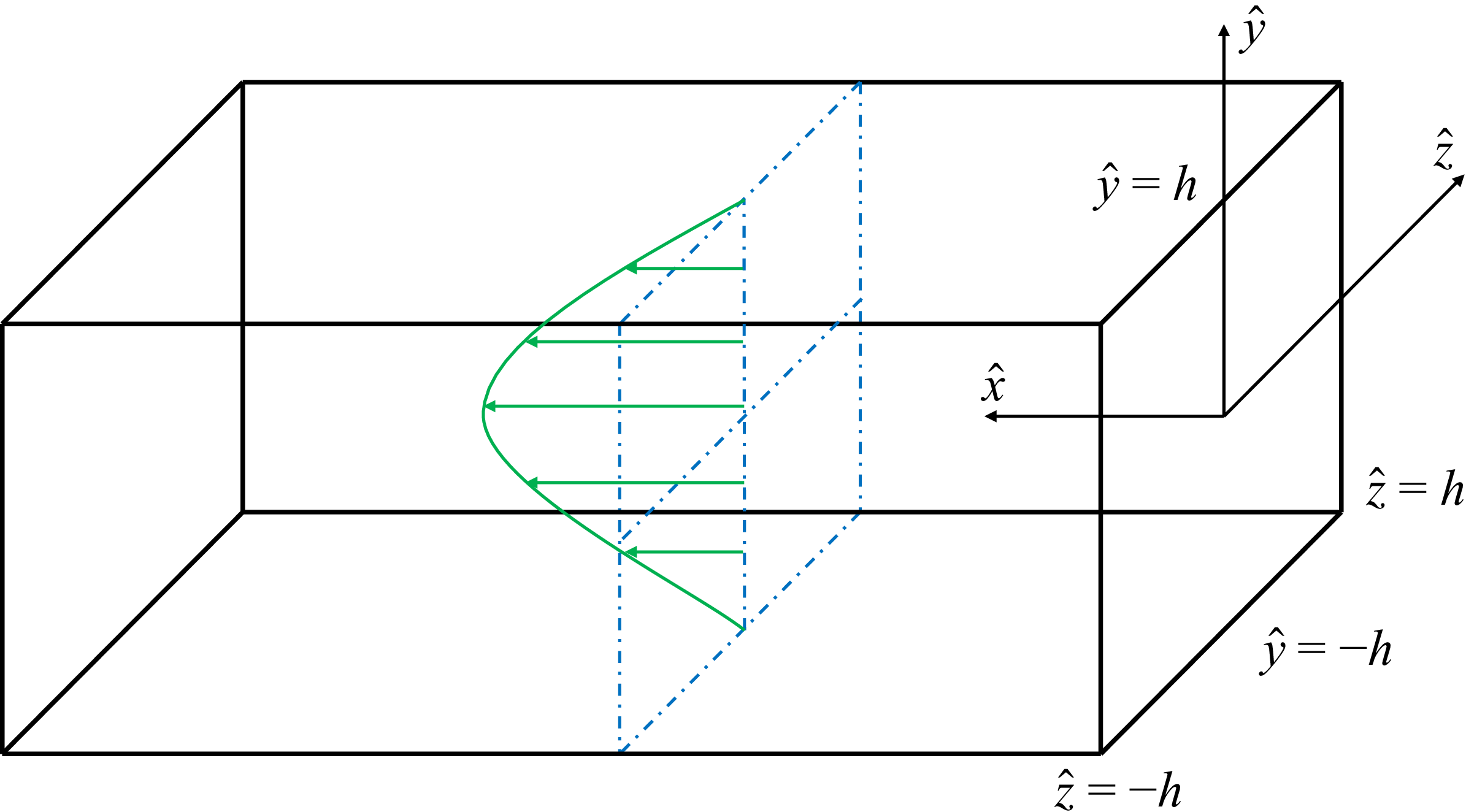
 h
 x
 y
 z=0
 y
 z

 Re=2796

 ϕ
 y
 z
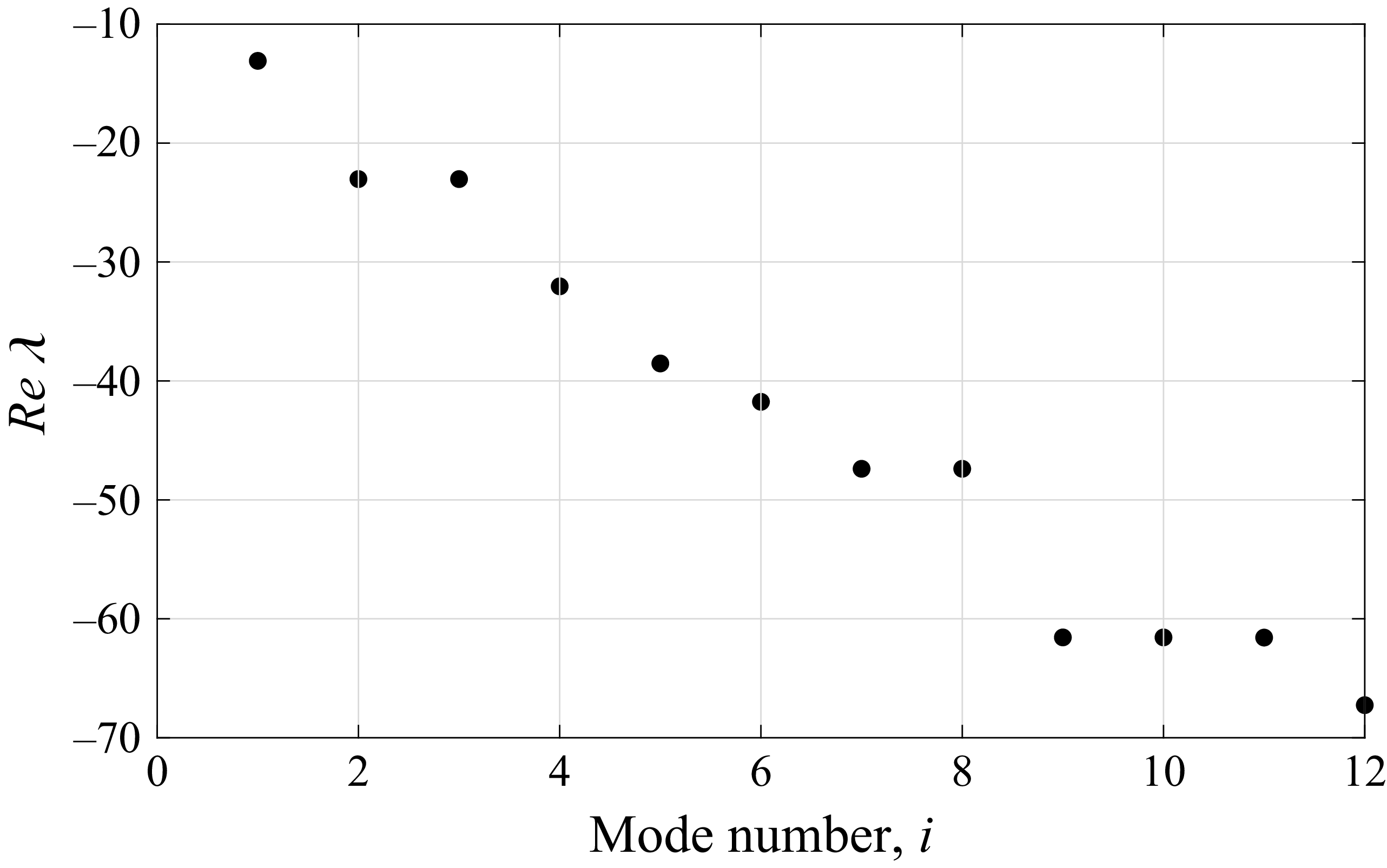
 Re
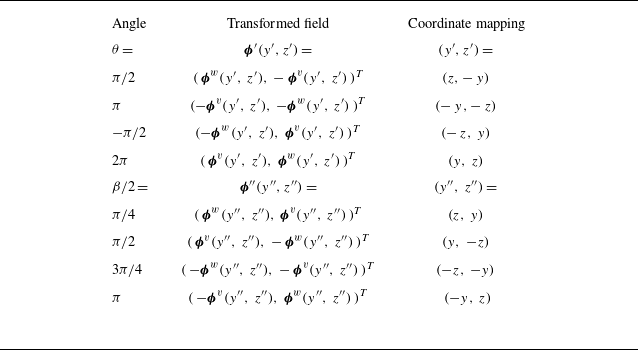
 ϕ(y,z)=(ϕv,ϕw)T
 R(θ)
 L(β)
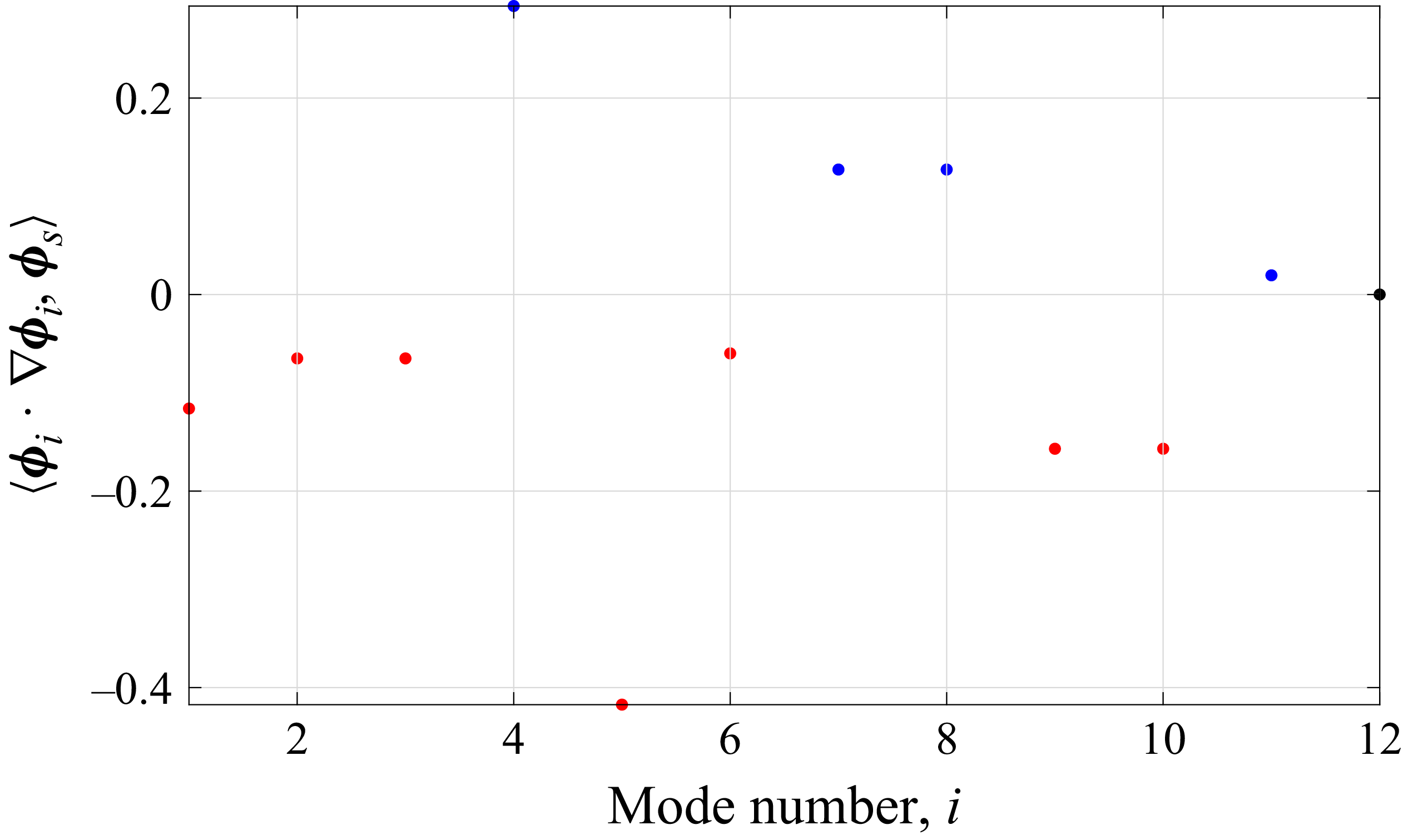
 ⟨ϕi⋅∇ϕi,ϕs⟩
 as
 i=1,2,…,12
 ⟨∇2ϕs,ϕs⟩<0
 as

 a1(t)
 as(t)
 95%
 0≤t≤2000
 0≤t≤800
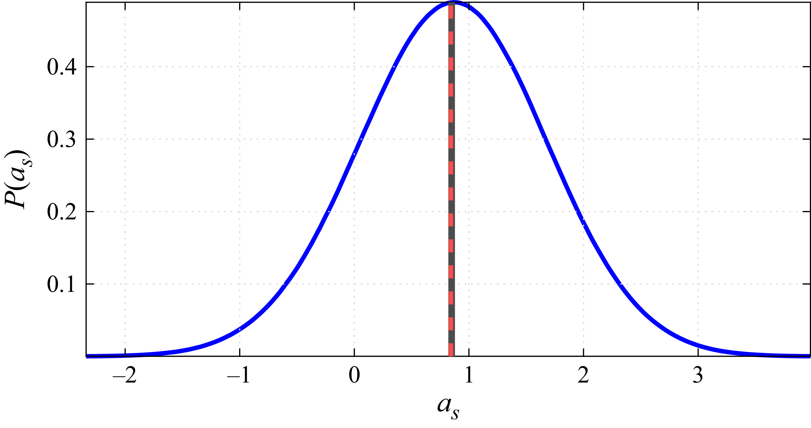
 as(t)
 as¯
 as¯
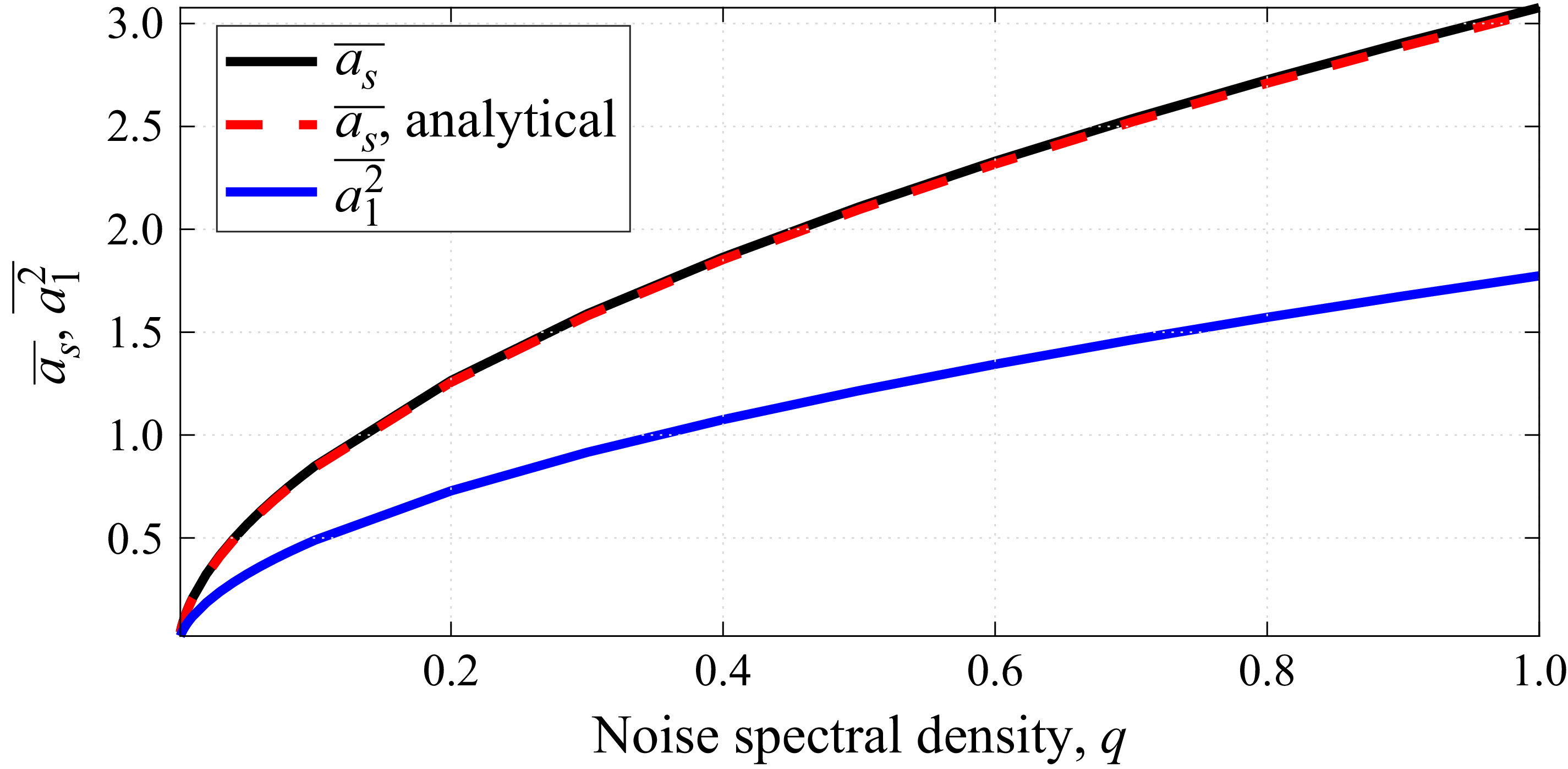
 as¯
 a12¯
 q
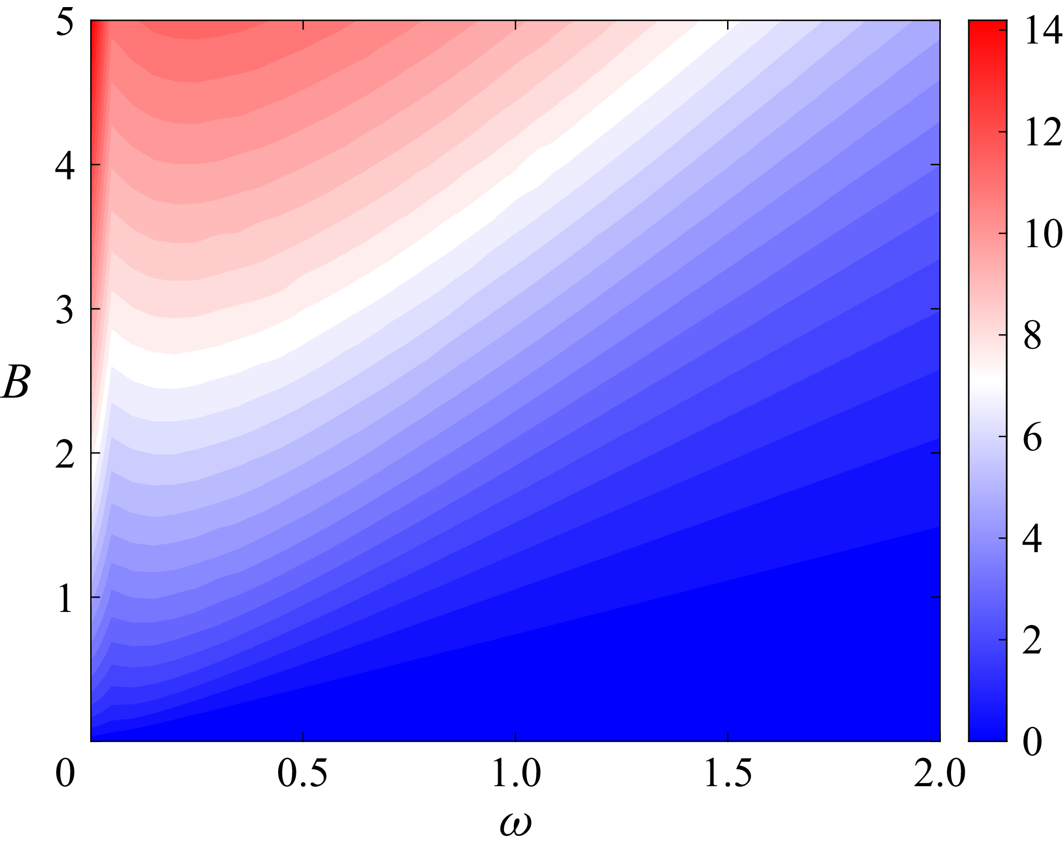
 as¯
 B
 ω
 f1=Bcos(ωt)

 ⟨ϕi⋅∇ϕj,ϕs⟩
 i
 j

 aiaj¯
 ai2¯
 ai¯
 q=0.1

 as¯
 N
 q=0.1

 ϕ4
 f4(t)=Bcos(t)
 aiaj¯
 ai¯
 B=0.1
 B=10

 as¯
 N
 f1=Bcost
 ϕ1
 B=0.1
 B=0.2
 B=0.3

 TA=350
 TA=500
 TA=1000

 B=0.01
 B=0.05
 B=0.1

 Ψ
 (ϕ1)
 B=0.01
 B=0.05
 B=0.1

 B=0.01
 B=10

 P1
 P2
 P1+P2
 Re=2796
 P2
 −1
 1
 N=22



