2. THE MODEL AND MODIFIED KPSS TEST

Consider the following DGP (cf. Müller and Elliott, 2003) for an observed series y_t

where ν_t is a stationary process. Here ρ_c,T = 1 − cT⁻¹, c ≥ 0. We wish to test the null hypothesis of local to unit root stationarity against the unit root alternative. Following Müller (2005) we state these as H₀ : c ≥ c > 0 against H₁ : c = 0 where c specifies the minimal amount of mean reversion under the stationary null hypothesis.

As regards the initial value, which is important under H₀, following Müller and Elliott (2003), we assume that it is fixed and set ξ = αω/(1 − ρ_c,T²)^1/2, for c > 0. Here α controls the magnitude of the initial value relative to the standard deviation of a stationary AR(1) process with parameter ρ_c,T < 1. We assume that ν_t is a zero mean stationary process with finite autocovariances E(ν_tν_t−j) = γ_j and long-run variance

that is finite and nonzero.

We consider the following generalized least squares (GLS) type transformation of the y_t based on our hypothesized value c under the stationary null:

for t = 2,…,T. To use the y_t − ρ_c,T y_t−1 as the basis for a KPSS test we need to make them invariant to μ(1 − ρ_c,T). So, we utilize the ordinary least squares (OLS) estimator of μ(1 − ρ_c,T) given by

and calculate the OLS residuals

Our modified KPSS test is then the standard KPSS statistic constructed from the r_c,t. That is,

Here

is any standard long-run variance estimator of the form

where λ(.) is a kernel function. The following theorem provides the asymptotic distribution of S^μ(c) under the null and alternative hypotheses.

THEOREM 1. Under the preceding assumption for ν_t,

where

and W(r) is a standard Wiener process. Also, when c = c > 0, H_α,c,c(r) = W(r) − rW(1).

The second part of the theorem shows that S^μ(c) has the standard intercept case KPSS limiting null distribution. Note that S^μ(c) is invariant to the initial value even in finite samples.¹

If (2) also includes a linear trend term, the modified statistic is formed from the OLS detrended y_t − ρ_c,T y_t−1, t = 2,…,T. Redefining r_c,t accordingly, the analogue to Theorem 1 follows by replacing H_α,c,c(r) with

. Also, S^μ(c) has the usual trend case KPSS distribution.

The modified KPSS test is related to the prewhitened long-run variance estimator suggested by Sul, Phillips, and Choi (2005) for the KPSS test. Instead of the usual fixed upper bound of 0.97 for the AR(1) prewhitening coefficient, they suggest using 1 − T^−1/2. The difference is that our AR(1) filtering uses 1 − cT⁻¹ and this is employed in both numerator and denominator of the test. Sul et al. (2005) note that the rate T⁻¹ at which 1 − cT⁻¹ approaches unity makes it inappropriate for prewhitening when used in the denominator alone, but clearly it is valid in our context.

3. COMPARISONS WITH OPTIMAL STATIONARITY TESTS

We compare the asymptotic performance of S^μ(c) with that of the stationarity test of Müller (2005), denoted Q^μ(g) in the notation of that paper (with g corresponding to c). This test is asymptotically optimal in a Gaussian setting when g = c, in the situation where the initial value is generated with α = 1. The test was originally suggested as a point optimal test of the unit root null in Elliott (1999) but can equally be considered as a test of the null of stationarity, simply by considering the opposite tail of the distribution to the unit root case.

When testing the unit root null, Müller and Elliott (2003) consider the effect that the magnitude of the initial value in a stationary series has on the power of unit root tests. In the current context of stationarity testing, this translates into an issue of size control. Elliott and Müller (2005), in the unit root testing context, derive an asymptotically optimal test (based on a weighted average power criterion) whose power varies little across different initial values. Again, it can equally be considered as a stationarity test, where size should be fairly robust across differing initial values. We denote this test Q^μ(g,k). As regards choosing parameters, we follow the previous authors and set c = g = 10 (k = 3.8).

Limit distributions of the three statistics are simulated by approximating the Wiener process functionals involved using i.i.d.N(0,1) variables, approximating the integrals by normalized sums of 5,000 steps. All experiments are based on 10,000 replications.

As in Müller (2005), we compare the tests by determining critical values for each such that rejection rates coincide at some prespecified value for c = 0 (power) and then examining their size for c > 0. In this way, one test dominates another if the former's rejection profile for c > 0 (size) lies consistently below that of the latter.²

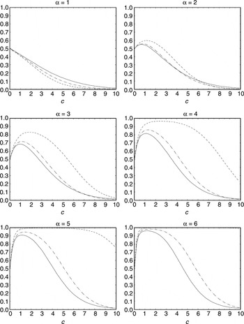
Figure 1 shows the rejection profiles of the tests across c for a rejection rate of 0.50 when c = 0. When α = 1, Q^μ(10) is the optimal test, and so it dominates the other two tests everywhere. Between Q^μ(10, 3.8) and S^μ(10), it is Q^μ(10, 3.8) that dominates, though not substantially. In fact, there is only ever a very modest amount of difference between the sizes of all three tests, with all having size close to zero when c = 10. The size of each test is also monotonically decreasing in c. For α > 1, the rejection profiles are no longer monotonic in c. There is always a region of c for which the size of each test is greater than power. However, this effect differs significantly across tests. As α increases the size of Q^μ(10) rapidly approaches 1.00 for most c, demonstrating its sensitivity to departures of the initial value from its optimality point. The other two test sizes appear much less sensitive to increasing α. Between these two, whereas there is virtually nothing to choose for α = 2, for all α ≥ 3 it is S^μ(10) that clearly dominates Q^μ(10, 3.8) in terms of exhibiting the least size distortion.

Asymptotic size and power: ———, Sμ(10); - - - - -, Qμ(10); – · – · –, Qμ(10, 3.8).

To compare finite-sample size, we consider the DGP (2) with μ = 0 and ν_t generated by the MA(1) model

with ε_t ∼ i.i.d.N(0,1). For Q^μ(10) and Q^μ(10, 3.8), we follow Müller (2005) and estimate ω² using residuals from an AR(1) regression of demeaned y_t in place of the r_c,t in (3). For all tests we use the quadratic spectral (QS) kernel for λ(.) and employ the automatic bandwidth selection of Newey and West (1994).

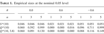
For T = 200 and c = 10, Table 1 shows the empirical size of the tests using nominal 0.05 level asymptotic null critical values for various values of θ and α.³

Empirical sizes at the nominal 0.05 level

Overall, our findings indicate that despite its optimality, Q^μ(10) is too susceptible to severe oversizing problems when α > 1 to be recommended for practical use. Although Q^μ(10, 3.8) suffers rather less in this same situation, it is still the case that S^μ(10) generally displays the more robust size control asymptotically for a given level of power and also has better finite-sample size properties. We therefore conclude that, in circumstances when there is some uncertainty about the generation of the initial value, the modified KPSS test is likely to provide the most dependable inference of those considered here.

4. PROOF OF THEOREM

As the r_c,t are invariant to μ, we can set μ = 0 without loss of generality, so that y_t = w_t. It also proves convenient to define z_t = w_t − w₁ and rewrite r_c,t in the form

Then

and we may write the first right-hand side term of (4) as

on noting that z₁ = 0. It is shown in Elliott (1999) that T^−1/2z_[rT] ⇒ ωK_α,c(r) where K_α,c(r) is defined as in Theorem 1 and W(r) is the Wiener process defined by

. So, setting t = [rT] we find that

For the second right-hand side term of (4), note that

Hence,

Thus, via the continuous mapping theorem,

That

follows simply by noting that for t = 2,…,T we can write

and so

To show the second part of the theorem note that when c = c > 0 we have, for t = 2,…,T,

and so r_c,t invariant to α and using standard results