2.1 Model bacterium

We consider a mono-flagellated bacterial swimmer near an infinite flat wall boundary in a Newtonian fluid of constant viscosity $\unicode[STIX]{x1D707}$ . The cell body is assumed to be a spheroid or a spherocylinder of minor semi-axes $a$ and principal axis $c$ ( $a\leqslant c$ ), including the spherical case. We denote the centre position of the cell body by $\boldsymbol{X}$ , and the bacterium is assumed to possess a single flagellum that is connected to one end of the major axis, as schematically illustrated in figure 1.

Figure 1.

Schematic picture of a model bacterium.

To describe the bacterial dynamics, we introduce three reference frames (Smith et al. Reference Smith, Gaffney, Blake and Kirkman-Brown2009; Ishimoto & Gaffney Reference Ishimoto and Gaffney2016): the laboratory frame $\{\boldsymbol{e}_{i}\}$ , the body-fixed frame $\{\boldsymbol{e}_{i}^{\prime }\}$ and the flagellum-fixed frame $\{\boldsymbol{e}_{i}^{\prime \prime }\}$ for $i=x,y,z$ . The body-fixed frame is obtained by a rotation of the laboratory frame by the rotation matrix $\unicode[STIX]{x1D63D}$ , given by $\unicode[STIX]{x1D609}_{ij}=\boldsymbol{e}_{i}\boldsymbol{\cdot }\boldsymbol{e}_{j}^{\prime }$ . The flagellum-fixed frame is obtained by a rotation of the body-fixed frame, and the rotation matrix $\unicode[STIX]{x1D641}$ is given by $\unicode[STIX]{x1D60D}_{ij}=\boldsymbol{e}_{i}^{\prime }\boldsymbol{\cdot }\boldsymbol{e}_{j}^{\prime \prime }$ . The origin of the body-fixed coordinates is set to be the centre of the cell body, and that of the flagellum-fixed coordinates is the connection point of the flagellum and the cell body, $\boldsymbol{x}_{c}$ . The swimmer surface $S$ is the union of the cell-body surface $S_{B}$ and flagellum surface $S_{F}$ , and we write the position vector $\boldsymbol{x}_{0}$ on the surface $S$ as

(2.1) $$\begin{eqnarray}\boldsymbol{x}_{0}=\left\{\begin{array}{@{}ll@{}}\boldsymbol{X}+(\boldsymbol{x}_{0}-\boldsymbol{X}),\quad & \boldsymbol{x}_{0}\in S_{B},\\ \boldsymbol{X}+(\boldsymbol{x}_{c}-\boldsymbol{X})+(\boldsymbol{x}_{0}-\boldsymbol{x}_{c}),\quad & \boldsymbol{x}_{0}\in S_{F}.\end{array}\right.\end{eqnarray}$$

The relative position vectors $\unicode[STIX]{x1D743}_{B}=\boldsymbol{x}_{0}-\boldsymbol{X}$ $(\boldsymbol{x}_{0}\in S_{B})$ and $\unicode[STIX]{x1D743}_{F}=\boldsymbol{x}_{0}-\boldsymbol{x}_{c}$ $(\boldsymbol{x}_{0}\in S_{F})$ can be obtained by the rotations,

(2.2a,b ) $$\begin{eqnarray}\unicode[STIX]{x1D743}_{B}=\unicode[STIX]{x1D63D}\boldsymbol{\cdot }\hat{\unicode[STIX]{x1D743}}_{B},\quad \unicode[STIX]{x1D743}_{F}=\unicode[STIX]{x1D63D}\boldsymbol{\cdot }\unicode[STIX]{x1D641}\boldsymbol{\cdot }\hat{\unicode[STIX]{x1D743}}_{F},\end{eqnarray}$$

where $\hat{\unicode[STIX]{x1D743}}_{B}$ and $\hat{\unicode[STIX]{x1D743}}_{F}$ are the components measured in the body-fixed and flagellum-fixed frames, respectively. The vectors are therefore constant in time. We then take the Lagrangian time derivative for the position vector, $\boldsymbol{x}_{0}$ , to derive the expressions of the velocity. Noting that only the rotation matrices are functions of time, we obtain

(2.3) $$\begin{eqnarray}\boldsymbol{v}(\boldsymbol{x}_{0})=\left\{\begin{array}{@{}ll@{}}\boldsymbol{U}+\unicode[STIX]{x1D734}\times (\boldsymbol{x}_{0}-\boldsymbol{X}),\quad & \boldsymbol{x}_{0}\in S_{B},\\ \boldsymbol{U}+\unicode[STIX]{x1D734}\times (\boldsymbol{x}_{c}-\boldsymbol{X})+(\unicode[STIX]{x1D63D}\boldsymbol{\cdot }\unicode[STIX]{x1D74E})\times (\boldsymbol{x}_{0}-\boldsymbol{x}_{c}),\quad & \boldsymbol{x}_{0}\in S_{F},\end{array}\right.\end{eqnarray}$$

where the linear and angular velocities are defined as $\dot{\boldsymbol{X}}=\boldsymbol{U}$ , $\dot{\unicode[STIX]{x1D63D}}=\unicode[STIX]{x1D734}\times \unicode[STIX]{x1D63D}$ and $\dot{\unicode[STIX]{x1D641}}=\unicode[STIX]{x1D74E}\times \unicode[STIX]{x1D641}$ , with the dots denoting the time derivatives.

We assume a cylindrical flagellum of radius $d$ , and, following Higdon (Reference Higdon1979) and Shum et al. (Reference Shum, Gaffney and Smith2010), consider a helical waveform of the flagellum whose centreline is given in terms of the flagellum-fixed coordinates ( $\hat{x}(\hat{z},t),{\hat{y}}(\hat{z},t),\hat{z}$ ) by

(2.4) $$\begin{eqnarray}\displaystyle & \displaystyle \hat{x}=A(1-\text{e}^{-k_{E}^{2}\hat{z}^{2}})\cos (k\hat{z}), & \displaystyle\end{eqnarray}$$

(2.5) $$\begin{eqnarray}\displaystyle & \displaystyle {\hat{y}}=-A(1-\text{e}^{-k_{E}^{2}\hat{z}^{2}})\sin (k\hat{z}). & \displaystyle\end{eqnarray}$$

Here, $A$ is the amplitude of the helix, $k$ is the wavenumber and the parameter $k_{E}$ governs the scale of the initial increase in the flagellar envelope. The functions (2.4) and (2.5) are defined within the range of $\hat{z}\in [0,L_{e}]$ , where the coordinate of the flagellar distal end, $L_{e}>0$ , is implicitly defined by

(2.6) $$\begin{eqnarray}L=\int _{0}^{L_{e}}\sqrt{1+\left(\frac{\text{d}\hat{x}}{\text{d}\hat{z}}\right)^{2}+\left(\frac{\text{d}{\hat{y}}}{\text{d}\hat{z}}\right)^{2}}\,\text{d}\hat{z}.\end{eqnarray}$$

2.2 Mechanical equations

Owing to the small size of the bacterial swimmer, one can neglect the inertia effects and thus the fluid motions obey the Stokes equation

(2.7) $$\begin{eqnarray}\unicode[STIX]{x1D735}p=\unicode[STIX]{x1D707}\unicode[STIX]{x0394}\boldsymbol{u},\end{eqnarray}$$

where $\boldsymbol{u}$ is the fluid velocity and $p$ is the pressure field. The fluid velocity can be represented by the single-layer boundary integral form (Pozrikidis Reference Pozrikidis2002; Shum & Gaffney Reference Shum and Gaffney2012)

(2.8) $$\begin{eqnarray}\boldsymbol{u}(\boldsymbol{x})=-\int _{S(\boldsymbol{x}_{0})}\unicode[STIX]{x1D642}(\boldsymbol{x},\boldsymbol{x}_{0})\boldsymbol{\cdot }\boldsymbol{q}(\boldsymbol{x}_{0})\,\text{d}S(\boldsymbol{x}_{0}).\end{eqnarray}$$

The integral kernel, $\unicode[STIX]{x1D642}$ , is the blakelet (Blake Reference Blake1971), which satisfies the zero velocity condition on the wall surface, $z=0$ , and the integral is performed over the entire cell surface, $S$ . Since the swimmer inertia is also negligible at low Reynolds number, the single-layer potential $\boldsymbol{q}(\boldsymbol{x}_{0})$ satisfies the force and torque balance equations, which read

(2.9) $$\begin{eqnarray}\int _{S(\boldsymbol{x}_{0})}[\boldsymbol{q}+\boldsymbol{f}_{ext}]\,\text{d}S(\boldsymbol{x}_{0})=\int _{S(\boldsymbol{x}_{0})}(\boldsymbol{x}_{0}-\boldsymbol{X})\times [\boldsymbol{q}(\boldsymbol{x}_{0})+\boldsymbol{f}_{ext}]\,\text{d}S(\boldsymbol{x}_{0})=\mathbf{0},\end{eqnarray}$$

where $\boldsymbol{f}_{ext}$ is the external force and will be considered for the cell–wall interactions. The no-slip boundary condition on the swimmer surface, $S$ , is given by $\boldsymbol{u}(\boldsymbol{x}_{0})=\boldsymbol{v}(\boldsymbol{x}_{0})$ and obtained from equations (2.3) and (2.8).

We consider a flexible hook that connects the cell body and the flagellum, modelling it as a torque spring following previous studies (Bennett et al. Reference Bennett, Lee, Anda, Nealson, Yildiz, O’Toole, Wong and Golestanian2016; de Anda et al. Reference de Anda, Lee, Lee, Bennet, Ji, Soltani, Harrison, Baker, Luo and Chou2017; Nguyen & Graham Reference Nguyen and Graham2017; Riley et al. Reference Riley, Das and Lauga2018). At the rigid limit of the hook, the flagellum is assumed to be connected normal to the body, or $\boldsymbol{e}_{z}^{\prime }=\boldsymbol{e}_{z}^{\prime \prime }$ . When the hook is flexible, the relative angle between the two vectors, $\boldsymbol{e}_{z}^{\prime }$ and $\boldsymbol{e}_{z}^{\prime \prime }$ , can take a non-zero value, but we assume that it eventually relaxes to zero by the hook torque spring. Let $f(\unicode[STIX]{x1D711})$ be the function that presents the magnitude of the recovery torque, where the angle $\unicode[STIX]{x1D711}$ is the relative angle, $\unicode[STIX]{x1D711}=\sin ^{-1}|\boldsymbol{e}_{z}^{\prime }\times \boldsymbol{e}_{z}^{\prime \prime }|$ . The bending torque due to the hook flexibility is therefore given by $\boldsymbol{M}_{bend}=-f(\unicode[STIX]{x1D711})\boldsymbol{e}_{\bot }^{\prime }$ , with the unit vector $\boldsymbol{e}_{\bot }^{\prime }$ given by $\boldsymbol{e}_{\bot }^{\prime }=\boldsymbol{e}_{z}^{\prime }\times \boldsymbol{e}_{z}^{\prime \prime }/|\boldsymbol{e}_{z}^{\prime }\times \boldsymbol{e}_{z}^{\prime \prime }|$ . With a positive constant $\unicode[STIX]{x1D705}$ , we assume $f(\unicode[STIX]{x1D711})=\unicode[STIX]{x1D705}\tan \unicode[STIX]{x1D711}$ , and thus the bending torque behaves as a linear torque spring with spring constant $\unicode[STIX]{x1D705}$ if the angle is small and diverges as the angle approaches $\unicode[STIX]{x03C0}/2$ , preventing the flagellum from penetrating to the cell body.

The flagellum is rotated by motor torque at the flagellar base, $\boldsymbol{M}_{mot}$ . In this study we assume a constant motor torque applied towards the normal to the cell-body surface, $\boldsymbol{M}_{mot}=\unicode[STIX]{x1D70F}\boldsymbol{e}_{z}^{\prime }$ (Shum & Gaffney Reference Shum and Gaffney2012; Shimogonya et al. Reference Shimogonya, Sawano, Wakabe, Inoue, Ishijima and Ishikawa2015; Jabbarzadeh & Fu Reference Jabbarzadeh and Fu2018).

Finally, we have the torque balance equation around the connection point $\boldsymbol{x}_{c}$ :

(2.10) $$\begin{eqnarray}\int _{S_{F}(\boldsymbol{x}_{0})}(\boldsymbol{x}_{0}-\boldsymbol{x}_{c})\times \boldsymbol{q}(\boldsymbol{x}_{0})\,\text{d}S_{F}(\boldsymbol{x}_{0})+\boldsymbol{M}_{bend}+\boldsymbol{M}_{mot}=\mathbf{0},\end{eqnarray}$$

noting that the surface integral should be computed only over the flagellar surface.

2.3 Wall conditions

In this study, we first fix the value of the separation distance between the wall boundary and the cell-body surface, $h$ . This assumption can be biologically interpreted by an attraction to a minimum of the surface potential, which ranges over the orders of $10{-}100~\text{nm}$ (Chen et al. Reference Chen, Busscher, van der Mei and Norde2011). We define the contact point, $\boldsymbol{X}_{p}$ , as the point on the cell body closest to the wall boundary, and let the angle of the cell-body inclination be $\unicode[STIX]{x1D703}=\cos ^{-1}(\boldsymbol{e}_{z}^{\prime }\boldsymbol{\cdot }\boldsymbol{e}_{z})\in [0,\unicode[STIX]{x03C0}]$ and consider the distance between the body centre and the wall boundary, $H(\unicode[STIX]{x1D703})$ , given by

(2.11) $$\begin{eqnarray}H(\unicode[STIX]{x1D703})=h+\left\{\begin{array}{@{}ll@{}}\sqrt{a^{2}\sin ^{2}\unicode[STIX]{x1D703}+c^{2}\cos ^{2}\unicode[STIX]{x1D703}}\quad & (\text{spheroid}),\\ a+(c-a)|\cos \unicode[STIX]{x1D703}|\quad & (\text{spherocylinder}).\end{array}\right.\end{eqnarray}$$

The $z$ component of the swimming velocity, $U_{z}$ , is geometrically determined by the constraint of constant separation, and this can be simply obtained (Moffatt & Shimomura Reference Moffatt and Shimomura2002; Moffatt et al. Reference Moffatt, Shimomura and Branicki2004) by

(2.12) $$\begin{eqnarray}U_{z}=\frac{\text{d}H}{\text{d}\unicode[STIX]{x1D703}}\frac{\text{d}\unicode[STIX]{x1D703}}{\text{d}t}=\left(\frac{\text{d}H}{\text{d}\unicode[STIX]{x1D703}}\right)\boldsymbol{e}_{\bot }\boldsymbol{\cdot }\unicode[STIX]{x1D734},\end{eqnarray}$$

where $\boldsymbol{e}_{\bot }$ is introduced by $\boldsymbol{e}_{\bot }=\boldsymbol{e}_{z}\times \boldsymbol{e}_{z}^{\prime }/|\boldsymbol{e}_{z}\times \boldsymbol{e}_{z}^{\prime }|$ . Note that the vector $\boldsymbol{e}_{\bot }$ becomes singular around $\unicode[STIX]{x1D703}\approx 0$ but the singular factor can be absorbed into the derivatives term in (2.12). From direct calculations, we have

(2.13) $$\begin{eqnarray}U_{z}=\left\{\begin{array}{@{}ll@{}}\displaystyle -\frac{(c^{2}-a^{2})\cos \unicode[STIX]{x1D703}}{H-h}(\boldsymbol{e}_{z}\times \boldsymbol{e}_{z}^{\prime })\boldsymbol{\cdot }\unicode[STIX]{x1D734}\quad & (\text{spheroid}),\\ -(c-a)\,\text{sgn}(\cos \unicode[STIX]{x1D703})(\boldsymbol{e}_{z}\times \boldsymbol{e}_{z}^{\prime })\boldsymbol{\cdot }\unicode[STIX]{x1D734}\quad & (\text{spherocylinder}).\end{array}\right.\end{eqnarray}$$

The velocity constraint relation (2.13) becomes discontinuous at $\unicode[STIX]{x1D703}=\unicode[STIX]{x03C0}/2$ for the spherocylindrical cell-body case, and we will terminate the numerical computation when the inclination angle approaches $\unicode[STIX]{x1D703}\approx \unicode[STIX]{x03C0}/2$ .

In the constant-separation situation, there are no boundary-related external forces in the horizontal direction. We thus set $\boldsymbol{f}_{ext}=(0,0,f_{ext})$ in the force and torque balance equations (2.9), and only hydrodynamic interactions are considered. In the $z$ direction, we have imposed zero velocity condition, $U_{z}=0$ , instead of the force balance equations.

Later in this paper, we will consider a fully three-dimensional numerical simulation, in which the cell is allowed to move in the perpendicular direction as well. At the very vicinity of the wall surface, the electrostatic potential is repulsive, and we assume the following short-range repulsive wall interactions per unit area of the cell surface (Ishikawa & Pedley Reference Ishikawa and Pedley2007; Spagnolie & Lauga Reference Spagnolie and Lauga2012; Ishimoto & Gaffney Reference Ishimoto and Gaffney2016):

(2.14) $$\begin{eqnarray}\boldsymbol{f}_{rep}(\boldsymbol{x})=g\frac{\text{e}^{-z/\unicode[STIX]{x1D706}}}{1-\text{e}^{-z/\unicode[STIX]{x1D706}}}\boldsymbol{e}_{z},\end{eqnarray}$$

where $g$ and $\unicode[STIX]{x1D706}$ are the strength and decay length of the wall repulsive force, respectively. The force decay length, therefore, provides the characteristic length of the minimum separation distance.

We also consider an adhesive attractive interaction between the cell-body surface and the wall, motivated by the nano-spring property of the pili adhesion of P. aeruginosa (Beaussart et al. Reference Beaussart, Baker, Kuchma, El-Kirat-Chatel, O’Toole and Dufren̂e2014). We simply model the adhesive interaction by an elastic bond, following the receptor–ligand binding between the sperm and the wall boundary (Ishimoto & Gaffney Reference Ishimoto and Gaffney2016). Elastic bonds are formed at each cell-body surface, $\boldsymbol{x}$ , once the distance from the wall is closer than $R_{on}$ , with the location of the bond $\boldsymbol{X}_{ad}$ given by $\boldsymbol{X}_{ad}=\boldsymbol{x}\boldsymbol{\cdot }(\mathbf{1}-\boldsymbol{e}_{z}\boldsymbol{e}_{z})+R_{ad}\boldsymbol{e}_{z}$ . The adhesive force is then assumed to be that of the linear spring,

(2.15) $$\begin{eqnarray}\boldsymbol{f}_{ad}(\boldsymbol{x})=-k(\boldsymbol{x}-\boldsymbol{X}_{ad}),\end{eqnarray}$$

where $k$ is the spring constant of the bond. The adhesive bond is, however, broken and removed when the bond length exceeds the length $R_{off}$ . Owing to the wall-associated forces, we set $\boldsymbol{f}_{ext}=\boldsymbol{f}_{rep}+\boldsymbol{f}_{ad}$ in the force and torque balance equations (2.9).

Figure 2.

(a) Schematic of a model bacterium with a spheroidal cell body. (b) Numerical meshes on a model bacterium surface with a spherocylindrical cell body.

2.4 Numerical methods

We solve the above set of equations via the boundary element method, following our previous studies (Ishimoto & Gaffney Reference Ishimoto and Gaffney2014, Reference Ishimoto and Gaffney2017). We discretize the cell-body surface using finer meshes near a contact point to resolve the hydrodynamic interactions efficiently (figure 2 b). We have discretized the cell body by 512 meshes and the flagellum by 186 meshes. The validation of the numerics is obtained by comparison with the asymptotic analysis of a sphere translated by a constant force (Goldmann, Cox & Brenner Reference Goldmann, Cox and Brenner1967), but the numerics loses its accuracy when the separation distance is too small ( $h/a\lesssim 0.003$ ). We also found that the use of half mesh size (fourfold total number of meshes) does not improve the resolution for the finer separation case. We therefore use the above number of meshes and only consider the separation distance with $h/a>0.003$ . With $N$ being the total number of the mesh elements on the swimmer surface, the equations can be reduced to a linear system with $3N+9$ degrees, and be solved instantaneously with respect to the unknown functions $\boldsymbol{q}$ , $\boldsymbol{U}$ , $\unicode[STIX]{x1D734}$ and $\unicode[STIX]{x1D74E}$ . The time evolutions of the swimmer dynamics are implemented via the Heun method.

In the simulation, we use a set of parameters representing a typical morphology of P. aeruginosa flagellum (Dasgupta, Arora & Ramphal Reference Dasgupta, Arora, Ramphal and Ramos2004) (see flagellum 1 of table 1). The parameters listed under flagellum 2 in table 1 correspond to a bacterial flagellum with an optimal power efficiency obtained by Shum et al. (Reference Shum, Gaffney and Smith2010) and used in our previous study (Ishimoto & Gaffney Reference Ishimoto and Gaffney2017). This parameter set will be used to check the robustness to the flagellar geometry and will be briefly considered in § 4.1.

Table 1.

List of the parameters of the model flagellum. As a model morphology of P. aeruginosa flagellum, we employ the parameter set of flagellum 1, and the parameters of flagellum 2 are used for a parameter robustness analysis.

We readily find characteristic scales for the length and the force, which are the flagellar length $L=1$ and fluid viscosity $\unicode[STIX]{x1D707}=1$ , respectively. The typical physical values of these unit scales are $L=10~\unicode[STIX]{x03BC}\text{m}$ and $\unicode[STIX]{x1D707}=1~\text{mPa}~\text{s}$ . The characteristic time scale of this system should be determined by the amount of the motor torque, which is estimated as ${\approx}2\times 10^{-18}~\text{N}~\text{m}$ (de Anda et al. Reference de Anda, Lee, Lee, Bennet, Ji, Soltani, Harrison, Baker, Luo and Chou2017). In this study, however, we will explore various sizes of cell body, and the time scale of the emerged swimming dynamics depends on cell geometry. Thus, except in § 3.2, we use $T=0.02~\text{s}$ as the physical unit of the time scale for convenience. In the numerical simulation, we non-dimensionalize the physical variables with the unit of $L=\unicode[STIX]{x1D707}=T=1$ .

3.1 Theoretical formulations

In this section, we approximate the flagellar dynamics by neglecting non-local hydrodynamic interactions, following the theoretical formulation by Ishimoto & Lauga (Reference Ishimoto and Lauga2019), in which they study elastohydrodynamic instability induced by the flexible hook for a multi-flagellated spherical bacterial cell in the absence of external boundaries.

We introduce the hydrodynamic drag and torque on the cell body, $\boldsymbol{F}_{body}$ and $\boldsymbol{M}_{body}$ , in the form of the linear relation

(3.1) $$\begin{eqnarray}\left(\begin{array}{@{}c@{}}\boldsymbol{F}_{body}\\ \boldsymbol{M}_{body}\end{array}\right)=\left(\begin{array}{@{}cc@{}}\unicode[STIX]{x1D63E}_{TT} & \unicode[STIX]{x1D63E}_{TR}\\ \unicode[STIX]{x1D63E}_{RT} & \unicode[STIX]{x1D63E}_{RR}\\ \end{array}\right)\left(\begin{array}{@{}c@{}}\boldsymbol{U}\\ \unicode[STIX]{x1D734}.\end{array}\right)\end{eqnarray}$$

The resistive matrix in (3.1) is diagonal for an axisymmetric cell body considered in this study if no external wall boundaries are considered. However, when the cell body is located near a wall boundary, the expressions of the resistive matrix are non-diagonal and the components are given as a function of the separation, $h$ . In this section, we only consider a spherical cell body and employ the asymptotic expression derived from the lubrication theory for a sphere in the vicinity of a wall boundary (Goldmann et al. Reference Goldmann, Cox and Brenner1967; Lauga et al. Reference Lauga, DiLuzio, Whiteside and Stone2006). The detailed expressions of the resistive matrix are provided in appendix A.

Similarly to § 2.2, we consider the force and torque balance equations for the whole cell and the flagellum, neglecting the non-local hydrodynamic interactions using the resistive force theory (Lauga & Powers Reference Lauga and Powers2009). We assume that the flagellum is a slender one-dimensional filament, and the flagellar shape is then determined by its tangent vector $\boldsymbol{t}(s)$ ( $s\in [0,L]$ ). From the resistive force theory, the hydrodynamic force on a segment of the flagellum, $\text{d}\boldsymbol{F}(s)$ , is linearly related to the local velocity, $\boldsymbol{v}$ in (2.3), as

(3.2) $$\begin{eqnarray}\text{d}\boldsymbol{F}(s)=[C_{t}\boldsymbol{t}\boldsymbol{t}+C_{n}(\mathbf{1}-\boldsymbol{t}\boldsymbol{t})]\boldsymbol{\cdot }\boldsymbol{v}(s)\,\text{d}s,\end{eqnarray}$$

where $C_{t}$ and $C_{n}$ are negative drag coefficients depending on the flagellar slenderness parameter. Introducing the position vector of the centreline of the flagellum relative to flagellar connecting point $\boldsymbol{x}_{c}$ as

(3.3) $$\begin{eqnarray}\unicode[STIX]{x1D743}(s)=\int _{0}^{s}\boldsymbol{t}(s^{\prime })\,\text{d}s^{\prime },\end{eqnarray}$$

we derive the hydrodynamic force on the flagellum, $\boldsymbol{F}$ , denoting the drag coefficient tensor in (3.2) by $\unicode[STIX]{x1D63E}$ :

(3.4) $$\begin{eqnarray}\boldsymbol{F}=\left[\int _{0}^{L}\unicode[STIX]{x1D63E}\,\text{d}s\right]\boldsymbol{\cdot }\boldsymbol{U}+\left[\int _{0}^{L}\unicode[STIX]{x1D63E}\boldsymbol{\cdot }\unicode[STIX]{x1D63C}\,\text{d}s\right]\boldsymbol{\cdot }\unicode[STIX]{x1D734}+\left[\int _{0}^{L}\unicode[STIX]{x1D63E}\boldsymbol{\cdot }\tilde{\unicode[STIX]{x1D63C}}\,\text{d}s\right]\boldsymbol{\cdot }\unicode[STIX]{x1D63D}\boldsymbol{\cdot }\unicode[STIX]{x1D74E}.\end{eqnarray}$$

Here, we have introduced skew matrices, $\unicode[STIX]{x1D63C}_{i}$ and $\tilde{\unicode[STIX]{x1D63C}}_{i}$ , whose components are, respectively, given by

(3.5a,b ) $$\begin{eqnarray}[\unicode[STIX]{x1D63C}]_{ij}=\unicode[STIX]{x1D700}_{ijk}((\boldsymbol{x}_{c}-\boldsymbol{X})_{k}+\unicode[STIX]{x1D709}_{k})\quad \text{and}\quad [\tilde{\unicode[STIX]{x1D63C}}]_{ij}=\unicode[STIX]{x1D700}_{ijk}\unicode[STIX]{x1D709}_{k},\end{eqnarray}$$

where $\unicode[STIX]{x1D700}_{ijk}$ is the Levi-Civita symbol. The force balance equations are obtained by summing up the forces:

(3.6) $$\begin{eqnarray}\boldsymbol{F}_{body}+\boldsymbol{F}=\mathbf{0}.\end{eqnarray}$$

Similarly to the above arguments, we then proceed to the torque balance around the centre of the cell body for an entire cell. We again neglect hydrodynamic interactions between the cell and flagella, and consider hydrodynamic drag on the flagella using the resistive force theory. The torque on a segment of a flagellum around the cell-body centre is given by $\text{d}\boldsymbol{M}=(\unicode[STIX]{x1D743}+(\boldsymbol{x}_{c}-\boldsymbol{X}))\times \text{d}\boldsymbol{F}$ , from which we obtain the torque expression by integrating $\text{d}\boldsymbol{M}$ over the flagellum,

(3.7) $$\begin{eqnarray}\boldsymbol{M}=\left[\int _{0}^{L}\unicode[STIX]{x1D63C}^{\text{T}}\boldsymbol{\cdot }\unicode[STIX]{x1D63E}\,\text{d}s\right]\boldsymbol{\cdot }\boldsymbol{U}+\left[\int _{0}^{L}\unicode[STIX]{x1D63C}^{\text{T}}\boldsymbol{\cdot }\unicode[STIX]{x1D63E}\boldsymbol{\cdot }\unicode[STIX]{x1D63C}\,\text{d}s\right]\boldsymbol{\cdot }\unicode[STIX]{x1D734}+\left[\int _{0}^{L}\unicode[STIX]{x1D63C}^{\text{T}}\boldsymbol{\cdot }\unicode[STIX]{x1D63E}\boldsymbol{\cdot }\tilde{\unicode[STIX]{x1D63C}}\,\text{d}s\right]\boldsymbol{\cdot }\unicode[STIX]{x1D63D}\boldsymbol{\cdot }\unicode[STIX]{x1D74E},\end{eqnarray}$$

where the superscript T indicates the transpose of a matrix. We thus have a torque balance equation for the whole cell,

(3.8) $$\begin{eqnarray}\boldsymbol{M}_{body}+\boldsymbol{M}=\mathbf{0}.\end{eqnarray}$$

Lastly, we consider the torque balance relation for the flagellum around the connection of the flagellum and the cell body. Incorporating hydrodynamic torque and elastic spring torque, we have the torque acting on a segment of a flagellum, which is given by $\text{d}\tilde{\boldsymbol{M}}=\unicode[STIX]{x1D743}\times \text{d}\boldsymbol{F}$ . Integration over the flagellum yields the hydrodynamic torque,

(3.9) $$\begin{eqnarray}\tilde{\boldsymbol{M}}=\left[\int _{0}^{L}\tilde{\unicode[STIX]{x1D63C}}^{\text{T}}\boldsymbol{\cdot }\unicode[STIX]{x1D63E}\,\text{d}s\right]\boldsymbol{\cdot }\boldsymbol{U}+\left[\int _{0}^{L}\tilde{\unicode[STIX]{x1D63C}}^{\text{T}}\boldsymbol{\cdot }\unicode[STIX]{x1D63E}\boldsymbol{\cdot }\unicode[STIX]{x1D63C}\,\text{d}s\right]\boldsymbol{\cdot }\unicode[STIX]{x1D734}+\left[\int _{0}^{L}\tilde{\unicode[STIX]{x1D63C}}^{\text{T}}\boldsymbol{\cdot }\unicode[STIX]{x1D63E}\boldsymbol{\cdot }\tilde{\unicode[STIX]{x1D63C}}\,\text{d}s\right]\boldsymbol{\cdot }\unicode[STIX]{x1D63D}\boldsymbol{\cdot }\unicode[STIX]{x1D74E}.\end{eqnarray}$$

We then have the torque balance equations for the flagellum,

(3.10) $$\begin{eqnarray}\tilde{\boldsymbol{M}}+\boldsymbol{M}_{elast}+\boldsymbol{M}_{mot}=\mathbf{0},\end{eqnarray}$$

where $\boldsymbol{M}_{mot}$ is the torque applied at a bacterium motor. In the current problem, the magnitude of the motor torque is assumed to be constant as discussed in the previous section.

The above set of governing equations (3.4)–(3.10) can be summarized into the following matrix form:

(3.11) $$\begin{eqnarray}\left(\begin{array}{@{}ccc@{}}\unicode[STIX]{x1D646}_{TT} & \unicode[STIX]{x1D646}_{TR} & \unicode[STIX]{x1D646}_{TF}\\ \unicode[STIX]{x1D646}_{RT} & \unicode[STIX]{x1D646}_{RR} & \unicode[STIX]{x1D646}_{RF}\\ \unicode[STIX]{x1D646}_{FT} & \unicode[STIX]{x1D646}_{FR} & \unicode[STIX]{x1D646}_{FF}\end{array}\right)\left(\begin{array}{@{}c@{}}\boldsymbol{U}\\ \unicode[STIX]{x1D734}\\ \unicode[STIX]{x1D63D}\boldsymbol{\cdot }\unicode[STIX]{x1D74E}\end{array}\right)=\left(\begin{array}{@{}c@{}}\mathbf{0}\\ \boldsymbol{ 0}\\ -\boldsymbol{M}_{elast}-\boldsymbol{M}_{motor}\end{array}\right),\end{eqnarray}$$

where the matrices on the left-hand side read

(3.12) $$\begin{eqnarray}\left(\begin{array}{@{}ccc@{}}\displaystyle \unicode[STIX]{x1D63E}_{TT}+\int _{0}^{L}\unicode[STIX]{x1D63E}\,\text{d}s & \displaystyle \unicode[STIX]{x1D63E}_{TR}+\int _{0}^{L}\unicode[STIX]{x1D63E}\boldsymbol{\cdot }\unicode[STIX]{x1D63C}\,\text{d}s & \displaystyle \int _{0}^{L}\unicode[STIX]{x1D63E}\boldsymbol{\cdot }\tilde{\unicode[STIX]{x1D63C}}\,\text{d}s\\ \displaystyle \unicode[STIX]{x1D63E}_{RT}+\int _{0}^{L}\unicode[STIX]{x1D63C}^{\text{T}}\boldsymbol{\cdot }\unicode[STIX]{x1D63E}\,\text{d}s & \displaystyle \unicode[STIX]{x1D63E}_{RR}+\int _{0}^{L}\unicode[STIX]{x1D63C}^{\text{T}}\boldsymbol{\cdot }\unicode[STIX]{x1D63E}\boldsymbol{\cdot }\unicode[STIX]{x1D63C}\,\text{d}s & \displaystyle \int _{0}^{L}\unicode[STIX]{x1D63C}^{\text{T}}\boldsymbol{\cdot }\unicode[STIX]{x1D63E}\boldsymbol{\cdot }\tilde{\unicode[STIX]{x1D63C}}\,\text{d}s\\ \displaystyle \int _{0}^{L}\tilde{\unicode[STIX]{x1D63C}}^{\text{T}}\boldsymbol{\cdot }\unicode[STIX]{x1D63E}\,\text{d}s & \displaystyle \int _{0}^{L}\tilde{\unicode[STIX]{x1D63C}}^{\text{T}}\boldsymbol{\cdot }\unicode[STIX]{x1D63E}\boldsymbol{\cdot }\unicode[STIX]{x1D63C}\,\text{d}s & \displaystyle \int _{0}^{L}\tilde{\unicode[STIX]{x1D63C}}^{\text{T}}\boldsymbol{\cdot }\unicode[STIX]{x1D63E}\boldsymbol{\cdot }\tilde{\unicode[STIX]{x1D63C}}\,\text{d}s\end{array}\right).\end{eqnarray}$$

3.2 Linear stability

We further simplify the bacterial model to perform linear stability analysis around the upright spinning motion. The typical flagellar rotation is sufficiently rapid compared with the time scale of the flagellar bending, and we approximate the flagellar propulsion by its time-averaged contribution (Lauga et al. Reference Lauga, DiLuzio, Whiteside and Stone2006). It then follows that the flagellar propulsion is axisymmetric around the flagellar long axis. Only in this section, we use the units of $a=\unicode[STIX]{x1D707}=\unicode[STIX]{x1D70F}=1$ for simplicity of mathematical expressions. In the context of the upright spinning motion of a bacterium with a spherical cell body, the emerged time scale is the rotation velocity of the cell body, and this is proportional to $\unicode[STIX]{x1D707}a^{3}/\unicode[STIX]{x1D70F}$ . In other words, we non-dimensionalize the system using this time scale.

Figure 3.

Schematic of the model bacterial cell. The flagellum is indicated in red. (a) Projection onto the $x$ – $z$ plane. The angle $\unicode[STIX]{x1D6FC}$ is the relative angle between $\boldsymbol{e}_{z}^{\prime }$ and $\boldsymbol{e}_{z}^{\prime \prime }$ , measured in the $x$ – $z$ plane. (b) Projection onto the $x$ – $y$ plane. The angle $\unicode[STIX]{x1D6FD}$ is measured in the $x$ – $y$ plane.

Following Ishimoto & Lauga (Reference Ishimoto and Lauga2019), we introduce $3\times 3$ matrices,

(3.13a-c ) $$\begin{eqnarray}\unicode[STIX]{x1D646}_{C}=\int _{0}^{L}\unicode[STIX]{x1D63E}\,\text{d}s,\quad \unicode[STIX]{x1D646}_{TF}=\int _{0}^{L}\unicode[STIX]{x1D63E}\boldsymbol{\cdot }\tilde{\unicode[STIX]{x1D63C}}\,\text{d}s,\quad \unicode[STIX]{x1D646}_{FF}=\int _{0}^{L}\tilde{\unicode[STIX]{x1D63C}}^{\text{T}}\boldsymbol{\cdot }\unicode[STIX]{x1D63E}\boldsymbol{\cdot }\tilde{\unicode[STIX]{x1D63C}}\,\text{d}s,\end{eqnarray}$$

and the axisymmetric flagellar propulsion enables us to simplify the expressions as

(3.14a-c ) $$\begin{eqnarray}\displaystyle \unicode[STIX]{x1D646}_{C}^{(0)}=\left(\begin{array}{@{}ccc@{}}k_{C} & 0 & 0\\ 0 & k_{C} & 0\\ 0 & 0 & K_{C}\end{array}\right),\quad \unicode[STIX]{x1D646}_{TF}^{(0)}=\left(\begin{array}{@{}ccc@{}}k_{D} & k_{T} & 0\\ -k_{T} & k_{D} & 0\\ 0 & 0 & K_{T}\end{array}\right),\quad \unicode[STIX]{x1D646}_{FF}^{(0)}=\left(\begin{array}{@{}ccc@{}}k_{F} & 0 & 0\\ 0 & k_{F} & 0\\ 0 & 0 & K_{F}\end{array}\right), & & \displaystyle \nonumber\\ \displaystyle & & \displaystyle\end{eqnarray}$$

where superscript ‘ $(0)$ ’ indicates the expressions in the flagellum-fixed frame so that the expression in the laboratory frame is transformed by $\unicode[STIX]{x1D646}_{C}=[\unicode[STIX]{x1D63D}\boldsymbol{\cdot }\unicode[STIX]{x1D641}]\boldsymbol{\cdot }\unicode[STIX]{x1D646}_{C}^{(0)}\boldsymbol{\cdot }[\unicode[STIX]{x1D63D}\boldsymbol{\cdot }\unicode[STIX]{x1D641}]^{-1}$ for instance. The symmetric nature of $\unicode[STIX]{x1D646}_{C}^{(0)}$ and $\unicode[STIX]{x1D646}_{FF}^{(0)}$ is inherited from the integrands. Note that the constants $k_{C}$ , $K_{C}$ , $k_{T}$ and $k_{F}$ are all negative values, and $k_{D}$ , $K_{T}$ and $K_{F}$ can be both positive and negative depending on the helicity of the flagellum. Detailed expressions for a helical flagellum are listed in appendix A.

The dynamics of the model bacteria possess six degrees of freedom associated with the rigid motion and two degrees of freedom associated with the angles, $\unicode[STIX]{x1D6FC}$ and $\unicode[STIX]{x1D6FD}$ , which designate the orientation of the rod flagellum (figure 3). With a constant separation from the wall boundary, we have in total eight degrees of freedom, and we will hereafter derive a linearized equation around the vertical spinning motion for the stability analysis.

We first decompose $\unicode[STIX]{x1D74E}=\unicode[STIX]{x1D641}\boldsymbol{\cdot }\unicode[STIX]{x1D74E}^{(0)}$ into tangential and normal components with respect to the flagellar axis $\boldsymbol{e}_{z}^{\prime \prime }$ as $\unicode[STIX]{x1D63D}\boldsymbol{\cdot }\unicode[STIX]{x1D74E}=\unicode[STIX]{x1D74E}_{t}+\unicode[STIX]{x1D74E}_{n}$ , where $\unicode[STIX]{x1D74E}_{t}\boldsymbol{\cdot }\boldsymbol{e}_{z}^{\prime \prime }=\unicode[STIX]{x1D714}_{0}$ and $\unicode[STIX]{x1D74E}_{n}\boldsymbol{\cdot }\boldsymbol{e}_{z}^{\prime \prime }=0$ . With $\unicode[STIX]{x1D64D}=\unicode[STIX]{x1D63D}\boldsymbol{\cdot }\unicode[STIX]{x1D641}$ , we introduce the flagellar rotation velocities in the flagellum-fixed coordinates, $\unicode[STIX]{x1D74E}_{t}^{(0)}$ and $\unicode[STIX]{x1D74E}_{n}^{(0)}$ , as $\unicode[STIX]{x1D74E}_{t}=\unicode[STIX]{x1D64D}\boldsymbol{\cdot }\unicode[STIX]{x1D74E}_{t}^{(0)}$ and $\unicode[STIX]{x1D74E}_{n}=\unicode[STIX]{x1D64D}\boldsymbol{\cdot }\unicode[STIX]{x1D74E}_{n}^{(0)}$ . Similarly, we can write the bending and motor torque expressions by the use of those in the flagellum-fixed coordinates as $\boldsymbol{M}_{elast}=\unicode[STIX]{x1D64D}\boldsymbol{\cdot }\boldsymbol{M}_{elast}^{(0)}$ and $\boldsymbol{M}_{motor}=\unicode[STIX]{x1D64D}\boldsymbol{\cdot }\boldsymbol{M}_{motor}^{(0)}$ .

Substituting these into (3.11), we obtain the effective cell-body dynamics,

(3.15) $$\begin{eqnarray}\left(\begin{array}{@{}ccc@{}}\unicode[STIX]{x1D646}_{TT} & \unicode[STIX]{x1D646}_{TR} & \unicode[STIX]{x1D646}_{TF}\\ \unicode[STIX]{x1D646}_{RT} & \unicode[STIX]{x1D646}_{RR} & \unicode[STIX]{x1D646}_{RF}\end{array}\right)\left(\begin{array}{@{}c@{}}\boldsymbol{U}\\ \unicode[STIX]{x1D734}\\ \unicode[STIX]{x1D74E}_{n}\end{array}\right)=\left(\begin{array}{@{}c@{}}-\unicode[STIX]{x1D646}_{TF}\boldsymbol{\cdot }\unicode[STIX]{x1D74E}_{t}\\ -\unicode[STIX]{x1D646}_{RF}\boldsymbol{\cdot }\unicode[STIX]{x1D74E}_{t}\\ \end{array}\right),\end{eqnarray}$$

where the right-hand side vector represents the force and torque generated by the flagellar propulsion. The equations of motion for the flagellar bending are calculated as

(3.16) $$\begin{eqnarray}\displaystyle & \displaystyle \unicode[STIX]{x1D64B}_{0}\boldsymbol{\cdot }\unicode[STIX]{x1D646}_{FT}^{(0)}\boldsymbol{\cdot }\unicode[STIX]{x1D64D}^{-1}\boldsymbol{\cdot }\boldsymbol{U}+\unicode[STIX]{x1D64B}_{0}\boldsymbol{\cdot }\unicode[STIX]{x1D64D}^{-1}\boldsymbol{\cdot }\unicode[STIX]{x1D646}_{FR}\boldsymbol{\cdot }\unicode[STIX]{x1D734}+\unicode[STIX]{x1D646}_{FF}^{(0)}\boldsymbol{\cdot }\unicode[STIX]{x1D74E}_{n}^{(0)}=-\boldsymbol{M}_{elast}^{(0)}-\unicode[STIX]{x1D64B}_{0}\boldsymbol{\cdot }\boldsymbol{M}_{motor}^{(0)},\qquad & \displaystyle\end{eqnarray}$$

(3.17) $$\begin{eqnarray}\displaystyle & \displaystyle \unicode[STIX]{x1D64C}_{0}\boldsymbol{\cdot }\unicode[STIX]{x1D646}_{FT}^{(0)}\boldsymbol{\cdot }\unicode[STIX]{x1D64D}^{-1}\boldsymbol{\cdot }\boldsymbol{U}+\unicode[STIX]{x1D64C}_{0}\boldsymbol{\cdot }\unicode[STIX]{x1D64D}^{-1}\boldsymbol{\cdot }\unicode[STIX]{x1D646}_{FR}\boldsymbol{\cdot }\unicode[STIX]{x1D734}+\unicode[STIX]{x1D646}_{FF}^{(0)}\boldsymbol{\cdot }\unicode[STIX]{x1D74E}_{t}^{(0)}=-\unicode[STIX]{x1D64C}_{0}\boldsymbol{\cdot }\boldsymbol{M}_{motor}^{(0)}, & \displaystyle\end{eqnarray}$$

after projection into the tangential (3.16) and normal (3.17) components with respect to $\boldsymbol{e}_{z}^{\prime \prime }$ , where $\unicode[STIX]{x1D64C}_{0}=\boldsymbol{e}_{z}\boldsymbol{e}_{z}$ and $\unicode[STIX]{x1D64B}_{0}=\mathbf{1}-\boldsymbol{e}_{z}\boldsymbol{e}_{z}$ are the projections onto the $\boldsymbol{e}_{z}$ axis and the $x{-}y$ plane.

Let $\unicode[STIX]{x1D64D}_{0}(\unicode[STIX]{x1D719},\boldsymbol{e})$ be a rotation matrix of degree $\unicode[STIX]{x1D719}$ around the vector $\boldsymbol{e}$ ; then the matrix $\unicode[STIX]{x1D641}$ can be expressed by $\unicode[STIX]{x1D641}\simeq \unicode[STIX]{x1D64D}_{0}(-\unicode[STIX]{x1D6FD},\boldsymbol{e}_{x})\boldsymbol{\cdot }\unicode[STIX]{x1D64D}_{0}(\unicode[STIX]{x1D6FC},\boldsymbol{e}_{y})$ for small angles, $\unicode[STIX]{x1D6FC}$ and $\unicode[STIX]{x1D6FD}$ . The local angular velocity can be obtained from the equation $\dot{\unicode[STIX]{x1D641}}=\unicode[STIX]{x1D74E}\times \unicode[STIX]{x1D641}$ , and we find $\unicode[STIX]{x1D74E}_{n}^{(0)}\simeq -\dot{\unicode[STIX]{x1D6FD}}\boldsymbol{e}_{x}+\dot{\unicode[STIX]{x1D6FC}}\boldsymbol{e}_{y}$ . Similarly, $\unicode[STIX]{x1D64D}=\unicode[STIX]{x1D63D}\boldsymbol{\cdot }\unicode[STIX]{x1D641}$ are calculated as

(3.18) $$\begin{eqnarray}\unicode[STIX]{x1D64D}=\left(\begin{array}{@{}ccc@{}}1 & 0 & \unicode[STIX]{x1D703}+\unicode[STIX]{x1D6FC}\\ 0 & 1 & \unicode[STIX]{x1D6FD}\\ -(\unicode[STIX]{x1D703}+\unicode[STIX]{x1D6FC}) & -\unicode[STIX]{x1D6FD} & 1\end{array}\right)+\text{higher-order terms}.\end{eqnarray}$$

Using these expressions, we estimate the leading-order contributions of (3.17), which reads

(3.19) $$\begin{eqnarray}K_{F}(\unicode[STIX]{x1D6FA}_{z}+\unicode[STIX]{x1D714}_{0})=-\unicode[STIX]{x1D70F},\end{eqnarray}$$

noting that we fix the boundary separation distance and thus $U_{z}=0$ . Similarly, from the last row of (3.15), we obtain the leading-order contributions

(3.20) $$\begin{eqnarray}(C_{R_{z}}+K_{F})\unicode[STIX]{x1D6FA}_{z}=-K_{F}\unicode[STIX]{x1D714}_{0}.\end{eqnarray}$$

Equations (3.19) and (3.20) provide the steady state that corresponds to the upright spinning motion, and we will consider the linearized equation around this equilibrium.

We begin by calculating the matrix entries in (3.15). By neglecting quadratic values of angles, we have

(3.21) $$\begin{eqnarray}\displaystyle \unicode[STIX]{x1D646}_{TT} & = & \displaystyle \left(\begin{array}{@{}ccc@{}}C_{D} & 0 & 0\\ 0 & C_{D} & 0\\ 0 & 0 & C_{D_{Z}}\end{array}\right)+\unicode[STIX]{x1D64D}\boldsymbol{\cdot }\unicode[STIX]{x1D646}_{C}^{(0)}\boldsymbol{\cdot }\unicode[STIX]{x1D64D}^{-1}\nonumber\\ \displaystyle & \simeq & \displaystyle \left(\begin{array}{@{}ccc@{}}C_{D}+k_{C} & 0 & (K_{C}-k_{C})(\unicode[STIX]{x1D703}+\unicode[STIX]{x1D6FC})\\ 0 & C_{D}+k_{C} & (K_{C}-k_{C})\unicode[STIX]{x1D6FD}\\ (K_{C}-k_{C})(\unicode[STIX]{x1D703}+\unicode[STIX]{x1D6FC}) & (K_{C}-k_{C})\unicode[STIX]{x1D6FD} & C_{D_{Z}}+K_{C}\end{array}\right),\end{eqnarray}$$

and, introducing the matrix $\unicode[STIX]{x1D63C}^{\prime }=\unicode[STIX]{x1D63C}-\tilde{\unicode[STIX]{x1D63C}}$ , we calculate

(3.22) $$\begin{eqnarray}\displaystyle \unicode[STIX]{x1D646}_{TR} & = & \displaystyle \left(\begin{array}{@{}ccc@{}}0 & -C_{S} & 0\\ C_{S} & 0 & 0\\ 0 & 0 & 0\end{array}\right)+\unicode[STIX]{x1D646}_{C}\boldsymbol{\cdot }\unicode[STIX]{x1D63C}^{\prime }+\unicode[STIX]{x1D646}_{TF}\nonumber\\ \displaystyle & \simeq & \displaystyle \left(\begin{array}{@{}ccc@{}}k_{D} & -C_{S}+(k_{C}+k_{T}) & -k_{T}\unicode[STIX]{x1D6FD}+K_{T}(\unicode[STIX]{x1D703}+\unicode[STIX]{x1D6FC})\\ C_{S}-(k_{C}+k_{T}) & k_{D} & k_{C}\unicode[STIX]{x1D703}+k_{T}(\unicode[STIX]{x1D703}+\unicode[STIX]{x1D6FC})+K_{T}\unicode[STIX]{x1D6FD}\\ \ast & \ast & K_{T}\end{array}\right).\end{eqnarray}$$

Here, the entries indicated by $\ast$ are of the order of $O(|\unicode[STIX]{x1D703}|,|\unicode[STIX]{x1D6FC}|,|\unicode[STIX]{x1D6FD}|)$ and therefore provide higher-order contributions to the $z$ component of the torque balance equation. We also obtain

(3.23) $$\begin{eqnarray}\displaystyle \unicode[STIX]{x1D646}_{RT} & = & \displaystyle \left(\begin{array}{@{}ccc@{}}0 & -C_{S}^{\prime } & 0\\ C_{S}^{\prime } & 0 & 0\\ 0 & 0 & 0\end{array}\right)+[\unicode[STIX]{x1D646}_{C}\boldsymbol{\cdot }\unicode[STIX]{x1D63C}^{\prime }+\unicode[STIX]{x1D646}_{TF}]^{\text{T}}\nonumber\\ \displaystyle & \simeq & \displaystyle \left(\begin{array}{@{}ccc@{}}k_{D} & -C_{S}^{\prime }+(k_{C}+k_{T}) & \ast \\ C_{S}^{\prime }-(k_{C}+k_{T}) & k_{D} & \ast \\ \ast & \ast & K_{T}\end{array}\right),\end{eqnarray}$$

and the entries shown by $\ast$ are the higher-order contributions that do not appear in the linearized equations. Combining the above expressions, we finally have

(3.24) $$\begin{eqnarray}\displaystyle \unicode[STIX]{x1D646}_{RR} & = & \displaystyle \left(\begin{array}{@{}ccc@{}}C_{R} & 0 & 0\\ 0 & C_{R} & 0\\ 0 & 0 & C_{R_{Z}}\end{array}\right)+\unicode[STIX]{x1D63C}^{\prime \,\text{T}}\boldsymbol{\cdot }\unicode[STIX]{x1D646}_{C}\boldsymbol{\cdot }\unicode[STIX]{x1D63C}^{\prime }+\unicode[STIX]{x1D63C}^{\prime \,\text{T}}\boldsymbol{\cdot }\unicode[STIX]{x1D646}_{FT}+\unicode[STIX]{x1D646}_{FT}\boldsymbol{\cdot }\unicode[STIX]{x1D63C}^{\prime }+\unicode[STIX]{x1D646}_{FF}\nonumber\\ \displaystyle & \simeq & \displaystyle \left(\begin{array}{@{}ccc@{}}\bar{C}_{R} & 0 & K_{R_{x}}\\ 0 & \bar{C}_{R} & K_{R_{y}}\\ K_{R_{x}} & K_{R_{y}} & C_{R_{z}}+K_{F}\end{array}\right),\end{eqnarray}$$

where $\bar{C}_{R}=C_{R}+k_{C}+2k_{T}+k_{F}$ , $K_{R_{x}}=-(k_{C}+k_{T})\unicode[STIX]{x1D703}+(K_{F}-k_{F}-k_{T})(\unicode[STIX]{x1D703}+\unicode[STIX]{x1D6FC})-K_{T}\unicode[STIX]{x1D6FD}$ and $K_{R_{y}}=K_{T}\unicode[STIX]{x1D6FC}+(K_{F}-k_{F}-k_{T})\unicode[STIX]{x1D6FD}$ .

The right-hand side of (3.15) is also calculated using $\unicode[STIX]{x1D714}^{(0)}=\unicode[STIX]{x1D714}_{0}\boldsymbol{e}_{z}$ as

(3.25) $$\begin{eqnarray}\displaystyle & \displaystyle \unicode[STIX]{x1D646}_{TF}\boldsymbol{\cdot }\unicode[STIX]{x1D74E}_{t}=\unicode[STIX]{x1D64D}\boldsymbol{\cdot }\unicode[STIX]{x1D646}_{TF}^{(0)}\boldsymbol{\cdot }(\unicode[STIX]{x1D714}_{0}\boldsymbol{e})_{z}=\unicode[STIX]{x1D714}_{0}K_{T}\{(\unicode[STIX]{x1D703}+\unicode[STIX]{x1D6FC})\boldsymbol{e}_{x}+\unicode[STIX]{x1D6FD}\boldsymbol{e}_{y}\}, & \displaystyle\end{eqnarray}$$

(3.26) $$\begin{eqnarray}\displaystyle & \displaystyle \unicode[STIX]{x1D646}_{RF}\boldsymbol{\cdot }\unicode[STIX]{x1D74E}_{t}=\unicode[STIX]{x1D714}_{0}K_{F}\{(\unicode[STIX]{x1D703}+\unicode[STIX]{x1D6FC})\boldsymbol{e}_{x}+\unicode[STIX]{x1D6FD}\boldsymbol{e}_{y}+\boldsymbol{e}_{z}\}+\unicode[STIX]{x1D714}_{0}K_{T}(-\unicode[STIX]{x1D6FD}\boldsymbol{e}_{x}+\unicode[STIX]{x1D6FC}\boldsymbol{e}_{y}). & \displaystyle\end{eqnarray}$$

We substitute these relations into (3.16) and (3.17), and finally obtain

(3.27) $$\begin{eqnarray}\left.\begin{array}{@{}c@{}}-k_{D}U_{x}+k_{T}U_{y}-(k_{T}+k_{F})\unicode[STIX]{x1D6FA}_{x}-k_{D}\unicode[STIX]{x1D6FA}_{y}+((k_{T}+k_{F})\unicode[STIX]{x1D703}+k_{F}\unicode[STIX]{x1D6FC})\unicode[STIX]{x1D6FA}_{z}+k_{F}\dot{\unicode[STIX]{x1D6FD}}=\unicode[STIX]{x1D705}\unicode[STIX]{x1D6FD}-M_{0}\unicode[STIX]{x1D6FC},\\ k_{T}U_{x}+k_{D}U_{y}-k_{D}\unicode[STIX]{x1D6FA}_{x}+(k_{T}+k_{F})\unicode[STIX]{x1D6FA}_{y}-k_{F}\unicode[STIX]{x1D6FD}\unicode[STIX]{x1D6FA}_{z}+k_{F}\dot{\unicode[STIX]{x1D6FC}}=\unicode[STIX]{x1D705}\unicode[STIX]{x1D6FC}+M_{0}\unicode[STIX]{x1D6FD}.\end{array}\right\}\end{eqnarray}$$

Noting that $\unicode[STIX]{x1D6FA}_{y}=\dot{\unicode[STIX]{x1D703}}$ and introducing $\dot{\boldsymbol{X}}=(U_{x},\dot{\unicode[STIX]{x1D703}},\dot{\unicode[STIX]{x1D6FC}},U_{y},\unicode[STIX]{x1D6FA}_{x},\dot{\unicode[STIX]{x1D6FD}})^{\text{T}}$ , these equations (3.21)–(3.26) can be summarized into the following matrix form:

(3.28) $$\begin{eqnarray}{\mathcal{A}}\dot{\boldsymbol{X}}={\mathcal{B}}\boldsymbol{X},\end{eqnarray}$$

with

(3.29) $$\begin{eqnarray}{\mathcal{A}}=\left(\begin{array}{@{}cc@{}}\unicode[STIX]{x1D63C}_{1} & \unicode[STIX]{x1D63C}_{3}\\ \unicode[STIX]{x1D63C}_{3}^{\text{ T}} & \unicode[STIX]{x1D63C}_{2}\end{array}\right),\end{eqnarray}$$

where $\unicode[STIX]{x1D63C}_{1}$ , $\unicode[STIX]{x1D63C}_{2}$ and $\unicode[STIX]{x1D63C}_{1}$ are $3\times 3$ matrices, given by

(3.30) $$\begin{eqnarray}\displaystyle & \displaystyle \unicode[STIX]{x1D63C}_{1}=\left(\begin{array}{@{}ccc@{}}C_{D}+k_{C} & -C_{S}+(k_{C}+k_{T}) & k_{T}\\ -C_{S}^{\prime }+(k_{C}+k_{T}) & C_{R}+k_{C}+2k_{T}+k_{F} & k_{T}+k_{F}\\ k_{T} & k_{T}+k_{F} & k_{F}\end{array}\right), & \displaystyle\end{eqnarray}$$

(3.31) $$\begin{eqnarray}\displaystyle & \displaystyle \unicode[STIX]{x1D63C}_{2}=\left(\begin{array}{@{}ccc@{}}C_{D}+k_{C} & C_{S}^{\prime }-(k_{C}+k_{T}) & k_{T}\\ C_{S}^{\prime }-(k_{C}+k_{T}) & C_{R}+k_{C}+2k_{T}+k_{F} & k_{T}+k_{F}\\ k_{T} & -(k_{T}+k_{F}) & k_{F}\end{array}\right), & \displaystyle\end{eqnarray}$$

(3.32) $$\begin{eqnarray}\displaystyle & \displaystyle \unicode[STIX]{x1D63C}_{3}=\left(\begin{array}{@{}ccc@{}}0 & k_{D} & -k_{D}\\ k_{D} & 0 & -k_{D}\\ k_{D} & -k_{D} & 0\end{array}\right), & \displaystyle\end{eqnarray}$$

and ${\mathcal{B}}$ is a $6\times 6$ matrix whose components are

(3.33) $$\begin{eqnarray}\displaystyle {\mathcal{B}}=\left(\begin{array}{@{}cccccc@{}}0 & -F_{e} & -F_{e} & 0 & 0 & k_{T}\unicode[STIX]{x1D6FA}_{z}\\ 0 & 0 & -F_{e} & 0 & 0 & (k_{T}+k_{F})\unicode[STIX]{x1D6FA}_{z}-M_{e}\\ 0 & 0 & \unicode[STIX]{x1D705} & 0 & 0 & k_{F}\unicode[STIX]{x1D6FA}_{z}+\unicode[STIX]{x1D70F}\\ 0 & -(k_{C}+k_{T})\unicode[STIX]{x1D6FA}_{z} & -k_{T}\unicode[STIX]{x1D6FA}_{z} & 0 & 0 & -F_{e}\\ 0 & (k_{C}+2k_{T}+k_{F})\unicode[STIX]{x1D6FA}_{z}-M_{e} & (k_{T}+k_{F})\unicode[STIX]{x1D6FA}_{z}-M_{e} & 0 & 0 & F_{e}\\ 0 & -(k_{T}+k_{F})\unicode[STIX]{x1D6FA}_{z} & -k_{F}\unicode[STIX]{x1D6FA}_{z}-\unicode[STIX]{x1D70F} & 0 & 0 & \unicode[STIX]{x1D705}\end{array}\right). & & \displaystyle \nonumber\\ \displaystyle & & \displaystyle\end{eqnarray}$$

In the expression (3.33), we have introduced the effective force and torque associated with the flagellar rotation by $F_{e}=K_{T}(\unicode[STIX]{x1D6FA}_{z}+\unicode[STIX]{x1D714}_{0})$ and $M_{e}=K_{F}(\unicode[STIX]{x1D6FA}_{z}+\unicode[STIX]{x1D714}_{0})$ , respectively.

From (3.33), it is readily found that the cell rigid motion obeys the angle dynamics, which can be obtained by inverting the matrix ${\mathcal{A}}$ as

(3.34) $$\begin{eqnarray}\frac{\text{d}}{\text{d}t}\left(\begin{array}{@{}c@{}}\unicode[STIX]{x1D703}\\ \unicode[STIX]{x1D6FC}\\ \unicode[STIX]{x1D6FD}\end{array}\right)=\unicode[STIX]{x1D63C}_{L}\left(\begin{array}{@{}c@{}}\unicode[STIX]{x1D703}\\ \unicode[STIX]{x1D6FC}\\ \unicode[STIX]{x1D6FD}\end{array}\right),\end{eqnarray}$$

and the eigenvalues of the matrix $\unicode[STIX]{x1D63C}_{L}$ provide the linear stability of the upright spinning motion.

Figure 4.

The largest real parts of the eigenvalues in the linear stability analysis for different cell-body size and hook rigidity. (a) The separation distance is $h/L_{e}=0.01$ and the flagellum is rotated by motor torque to push forwards to the cell body (pusher). (b) The separation distance is $h/L_{e}=0.001$ and the flagellum rotation direction is the same (pusher) as in (a). (c) The flagellar rotation direction is inverted (puller) from (a,b) with the separation distance, $h/L_{e}=0.01$ . (d) The separation distance is $h/L_{e}=0.001$ and the flagellar rotation direction is the same (puller) as in (c).

In figure 4, the largest real parts of the eigenvalues are plotted for different values of the cell-body size $L_{e}/a$ and dimensionless hook rigidity $\unicode[STIX]{x1D705}/\unicode[STIX]{x1D70F}$ . The effective length of the axisymmetric flagellum is $L_{e}\approx 0.85L$ for the parameters of the model P. aeruginosa (flagellum 1 in table 1). The separation distance from the boundary is $h/L_{e}=0.01$ for figure 4(a,c) and $h/L_{e}=0.001$ for figure 4(b,d). When $\unicode[STIX]{x1D70F}>0$ , the flagellum generates a force towards the cell body, as of pushers, and the results are shown in figure 4(a,b). With a negative $\unicode[STIX]{x1D70F}$ , the rotation direction of the flagellum is inverted, and the propulsive force pulls away from the cell body, as of pullers, and figure 4(c,d) correspond to this case.

As seen in figure 4, the linear stability dramatically differs between the pusher and puller flagella, and the pusher flagellum can be stable only when the dimensionless rigidity ranges in an intermediate magnitude, $\unicode[STIX]{x1D705}/\unicode[STIX]{x1D70F}\sim 1$ . In contrast, the puller flagellum case is found to be stable in a broad range of the cell-body size and hook rigidity. The stability phase map, however, is not rigorously symmetric, reflecting the breakdown of the pusher–puller duality by the flexibility of the hook. With a completely rigid flagellum, the swimming stability is shown to be opposite between the pusher and the corresponding puller from the time-reversal symmetry of the Stokes equations (Ishimoto & Gaffney Reference Ishimoto and Gaffney2013). The effects of the separation distance are more significant in the pusher cases, and the parameter regions for stable spinning motions are broadened as the cell body approaches the boundary.

Figure 5.

The largest real parts of the eigenvalues in the linear stability analysis neglecting either the force or torque contribution from the flagellar propulsion. The separation distance is $h/L_{e}=0.01$  (a–c) and $h/L_{e}=0.001$  (d–f). Panels (a,d) and (b,e) show the linear stability for the flagellum without torque exertion (pushing force only, pulling force only), and panels (c,f) correspond to the results for the flagellum without force exertion (torque only).

The linearized problem (3.34) contains both the force and torque contributions of the flagellar propulsion. To examine the mechanisms underlying the non-trivial stability phase map, we will theoretically separate the force and torque contributions.

We first consider the contribution from the flagellar force exertion, dropping the flagellar torque effects by setting $\unicode[STIX]{x1D6FA}_{z}=0$ and $M_{e}=0$ while keeping $F_{e}$ being non-zero in the matrix ${\mathcal{B}}$ . The sign of $\unicode[STIX]{x1D70F}$ determines whether the flagellum is a pusher or a puller. We calculate the largest real parts of the eigenvalues in the linear problem without torque terms, and the results are plotted in figure 5(a,b) for the case of $h/L_{e}=0.01$ , and in figure 5(d,e) when $h/L_{e}=0.001$ . As shown in figure 5(a,d) (pushing force only), the stability of a pushing flagellar bacterium is not as simple as previously considered (Lauga et al. Reference Lauga, DiLuzio, Whiteside and Stone2006; Petroff & Libchaber Reference Petroff and Libchaber2018), whereas a puller flagellum stabilizes the upright position in a wider range of parameters (figure 5 b,e, pulling force only).

To provide physical interpretations for the problem without the torque effects, we again consider the full problem of (3.34), where the expression of the matrix $\unicode[STIX]{x1D63C}_{L}$ requires the inverse of the $6\times 6$ matrix ${\mathcal{A}}$ . When the flagellar chirality effects $k_{D}$ can be negligible, the matrix inverse can be simplified, since the off-diagonal block $\unicode[STIX]{x1D63C}_{3}$ vanishes. In the realistic bacterial flagellar shape, this term is typically very small, with the relative magnitude of the order of $O(10^{-2})$ compared with the other terms (Ishimoto & Lauga Reference Ishimoto and Lauga2019). We therefore temporarily neglect the chirality effects by $k_{D}=0$ and consider the mathematical structures of the linear equation (3.34). Even with this simplification, the dynamics are still complicated since the angle $\unicode[STIX]{x1D6FD}$ dynamics is strongly coupled with the entire motion as seen in the right-most column of (3.33). With further simplification by assuming that the angle $\unicode[STIX]{x1D6FD}$ is decoupled from the entire dynamics, considering the hook being allowed to bend in one direction, we can reduce (3.34) to the form

(3.35) $$\begin{eqnarray}\frac{\text{d}}{\text{d}t}\left(\begin{array}{@{}c@{}}\unicode[STIX]{x1D703}\\ \unicode[STIX]{x1D6FC}\end{array}\right)=\unicode[STIX]{x1D63C}_{0}\left(\begin{array}{@{}c@{}}\unicode[STIX]{x1D703}\\ \unicode[STIX]{x1D6FC}\end{array}\right),\end{eqnarray}$$

which coincides with the dynamics without the flagellar torque effects under the assumption of negligible chirality effects, and therefore the maximum eigenvalue of the matrix $\unicode[STIX]{x1D63C}_{0}$ is very close to the plots shown in figure 5(a,b,d,e). The force contribution can therefore be interpreted as the dynamics without the dynamics associated with the angle  $\unicode[STIX]{x1D6FD}$ .

As in figure 5(a,d), except for the region with $\unicode[STIX]{x1D705}/\unicode[STIX]{x1D70F}\sim 1$ in the pusher flagellum case, the stability is mainly determined by the flagellar length $L_{e}/a$ , and this can be simply understood by analysing the rigid hook limit ( $\unicode[STIX]{x1D705}\rightarrow \infty$ ). Let us again go back to the full problem (3.34) and neglect the small chirality effects for brevity. We can dismiss the dynamics of the angles $\unicode[STIX]{x1D6FC}$ and $\unicode[STIX]{x1D6FD}$ at the rigid hook limit, and the stability can be obtained by the two-dimensional linear problem,

(3.36) $$\begin{eqnarray}\left(\begin{array}{@{}cc@{}}C_{D}+k_{C} & -C_{S}+(k_{C}+k_{T})\\ -C_{S}^{\prime }+(k_{C}+k_{T}) & C_{R}+k_{C}+2k_{T}+k_{F}\end{array}\right)\left(\begin{array}{@{}c@{}}U_{x}\\ \dot{\unicode[STIX]{x1D703}}\end{array}\right)=\left(\begin{array}{@{}c@{}}F_{e}\unicode[STIX]{x1D703}\\ 0\end{array}\right).\end{eqnarray}$$

Inverting the matrix on the left-hand side, we obtain the time evolution of angle  $\unicode[STIX]{x1D703}$ ,

(3.37) $$\begin{eqnarray}\frac{\text{d}\unicode[STIX]{x1D703}}{\text{d}t}=-\frac{F_{e}}{\unicode[STIX]{x1D6E5}_{r}}[C_{S}^{\prime }-(k_{C}+k_{T})]\unicode[STIX]{x1D703},\end{eqnarray}$$

where $\unicode[STIX]{x1D6E5}_{r}$ is the determinant of the $2\times 2$ matrix of (3.36) and is a positive value.

The longer flagellum experiences a large hydrodynamic drag that orients the cell towards the wall boundary as $k_{C}=O(L_{e})$ and $k_{T}=O(L_{e}^{2})$ , whereas $C_{S}^{\prime }$ is independent of $L_{e}$ and behaves as $O(a^{3}\log (a/h))$ from the lubrication theory (see also appendix A). We therefore obtain a critical flagellar length $L_{e}^{\ast }$ as a function of separation distance $h$ , above which the vertical spinning configuration becomes unstable for the pusher flagellum case. From the time-reversal symmetry of the Stokes equations, the critical value provides the lower limit of the flagellar length for a stable spinning top with a puller flagellum at the rigid limit. Further, these results indicate that the rigid hook model cannot exhibit a stable spinning top motion if the flagellum length is reasonably long as in a real bacterial swimmer ( $L_{e}/a\sim 10$ ).

We then consider the contribution from the flagellar torque exertion. We drop the flagellar force effects simply by setting $F_{e}=0$ and keep $\unicode[STIX]{x1D6FA}_{z}$ and $M_{e}$ being non-zero in the matrix ${\mathcal{B}}$ . As in the flagellar force contribution, we compute the largest real parts of the eigenvalues of the linear problem with the flagellar force terms. The results are plotted in figure 5(c) for the case of $h/L_{e}=0.01$ and figure 5(f) for the case of $h/L_{e}=0.001$ . Note that the stability is independent of the sign of $\unicode[STIX]{x1D70F}$ due to the symmetry.

From these plots (figure 5 c,f), it is found that the torque due to the flagellar propulsion contributes to the stabilization of the upright spinning motion in a large parameter region, and, in particular, with the intermediate hook rigidity, $\unicode[STIX]{x1D705}/\unicode[STIX]{x1D70F}\sim 1$ , the dynamical stabilization is promoted for a relatively smaller cell body (or a longer flagellum), including the biologically relevant parameter regimes $L_{e}/a\sim 10$ . The hook rigidity of P. aeruginosa has been estimated as $\unicode[STIX]{x1D705}/\unicode[STIX]{x1D70F}\approx 2$ (de Anda et al. Reference de Anda, Lee, Lee, Bennet, Ji, Soltani, Harrison, Baker, Luo and Chou2017), which remarkably lies in the region where the vertical spinning motion is strongly stabilized.

Figure 6.

The summation of the largest real parts of the eigenvalues from the force-only and torque-only problems for a pusher flagellum. (a) Plots obtained by the summation of the values in figure 5(a,c), where the separation distance is $h/L_{e}=0.01$ . (b) Plots obtained by the summation of the values in figure 5(d,f), where the separation distance is $h/L_{e}=0.001$ .

Figure 6(a,b) indicates the summations of the largest real parts of the eigenvalues from the force-only and torque-only problems in figure 5. In figure 6(a), the sum of the values of figures 5(a) and 5(c) are shown. This stability map for the pusher flagellum with $h/L_{e}=0.01$ is almost the same as the full linear problem in figure 4(a). Similarly, the sum of the values of figures 5(d) and 5(f) are shown in figure 6(a) for the pusher flagellum with $h/L_{e}=0.001$ . We find a remarkable coincidence on the stability map between the full problem and the sum of the force-only and torque-only problems. We can thus understand the full stability analysis in figure 4 by the separate effects of the flagellar force and torque contributions shown in figure 5.

These enable us to simply interpret the mechanical stability of the vertical spinning motion as the competition between the flagellar force and torque contributions. With the counter-rotating pulling flagellum, the flagellar propulsive force contributes to the stable vertical motion, whereas the propulsive force contributes to destabilizing the spinning motion in the pusher flagellar case. In a limited but biologically relevant parameter region, however, the torque stabilization effects are dominating compared with the force destabilization effect, hence the vertical spinning results in a mechanically stable state.

4.1 Spherical cell body

The linear stability analysis based on the local interaction theory in the previous section has suggested that the spherical cell body with a pusher flagellum can be stabilized only when the magnitudes of the flagellar bending torque and induced motor torque are comparable, i.e.  $\unicode[STIX]{x1D705}/\unicode[STIX]{x1D70F}\sim 1$ . We will see how the full hydrodynamic interactions could be explained by the local interaction theory.

Figure 7.

Swimming behaviours of a model bacterium with a spherical cell body and a pusher flagellum with constant separation distances of (a)  $h/L=0.01$ and (b)  $h/L=0.001$ . For each parameter value, the simulations have been done with two different initial angles, $\unicode[STIX]{x1D703}_{init}=0.1\unicode[STIX]{x03C0}$ and $\unicode[STIX]{x1D703}_{init}=0.25\unicode[STIX]{x03C0}$ . We enclose by dashed lines the region with stable upright spinning motions, which contains the cases when stable vertical motions are observed from both initial angle conditions (red upright triangle ▴) and only the shallow initial angle (green diamond ♦). The upright spinning motion cannot be realized in the parameter regions indicated by blue down triangles (▾). In the region indicated by black rectangles (▪), the inclination angle $\unicode[STIX]{x1D703}$ approaches a non-zero value, and the bacterium exhibits a non-vertical spinning motion.

Figure 8.

Dynamics of a model bacterial swimmer with a spherical cell body of radius $a/L=c/L=0.15$ . The motor torque is given by a non-dimensional value of $0.04$ , and the results of different hook rigidity $\unicode[STIX]{x1D705}/\unicode[STIX]{x1D70F}=\{10,3,1,0.3\}$ are shown. The separation distance is fixed as $h/L=0.001$ . (a,b) The time evolutions of the cell-body inclination angle $\unicode[STIX]{x1D703}$  (a) and the flagellar bending angle $\unicode[STIX]{x1D711}$  (b) are plotted in units of $\unicode[STIX]{x03C0}$ . (c,d) The trajectories of the cell-body centre for the same simulations are shown in a closer view (c) and in a wider view (d). The simulation of $\unicode[STIX]{x1D705}/\unicode[STIX]{x1D70F}=0.3$ had to be terminated around the non-dimensional time of 100–200, as the flagellum approaches much too close to the boundary.

Figure 9.

Dynamics of a model bacterial swimmer with a spherical cell body, as in figure 8, but with a smaller radius $a/L=c/L=0.1$ . The motor torque is given by a non-dimensional value of $0.04$ , and the results of different hook rigidity $\unicode[STIX]{x1D705}/\unicode[STIX]{x1D70F}=\{10,3,1,0.3\}$ are shown. (a,b) The separation distance is fixed as $h/L=0.001$ . The time evolutions of the cell-body inclination angle $\unicode[STIX]{x1D703}$  (a) and the flagellar bending angle $\unicode[STIX]{x1D711}$  (b) are plotted in units of $\unicode[STIX]{x03C0}$ . (c,d) The trajectories of the cell-body centre for the same simulations are shown in a closer view (c) and in a wider view (d).

Following figure 4, the swimming behaviours have been numerically examined for different cell body/flagellar length ratio $a/L$ and hook rigidity $\unicode[STIX]{x1D705}/\unicode[STIX]{x1D70F}$ . At each parameter value, we have performed numerical simulations with two different initial conditions of the shallow initial angle $\unicode[STIX]{x1D703}_{init}=0.1\unicode[STIX]{x03C0}$ and steeper angle $\unicode[STIX]{x1D703}_{init}=0.25\unicode[STIX]{x03C0}$ . Throughout this paper, the initial position of the cell-body centre satisfies $x/L=y/L=0$ , and the initial bending angle is set to be zero, i.e.  $\unicode[STIX]{x1D711}_{init}=0$ .

The stability diagrams are summarized in figure 7 for the different separation distances, $h/L=0.01$ and $0.001$ . Depending on the long-time behaviours obtained from the numerical simulations, the dynamics are categorized into the four groups, which are plotted in different colours and symbols. The red upright triangles (▴) indicate that the stable vertical spinning motion is realized from the two different initial angles. In the parameters indicated by the green diamonds (♦), only the shallow initial angle case has exhibited the stable upright motion, and the steeper initial angle has resulted in a wall-following behaviour, whereas the cell has moved along the boundary for both the initial angles in the parameter regions indicated by the blue down triangles (▾). The black squares (▪) represent the cases where the upright spinning motion is obtained but the inclination angle approaches a non-trivial angle.

The regions enclosed by the dashed lines in figure 7 contain the parameter sets for the stable upright spinning motion, which may correspond to the linear stable regions obtained in the local interaction theory. We found remarkable agreement between the local interaction theory and the full numerical simulation. In particular, the enhancement of the stability by the intermediate hook rigidity, $\unicode[STIX]{x1D705}/\unicode[STIX]{x1D70F}\sim 1$ , has been successfully predicted by the linear stability theory. Nevertheless, the stable behaviours in the very flexible parameter regions are not explained by the local interaction theory. In these parameter regions, the flagellar bending angles are oscillatory in time (see also figures 8 and 9), and the axisymmetric flagellar propulsion model would not be a feasible assumption. Another subtle disagreement between the theory and simulation can be found in the enlargement of the stable region with large values of $L_{e}/a$ . The eigenvalue plots in figure 4 indicate that vertical motion is weakly stable in this region, and thus the simulation may have missed the basin of the weak attractor.

In contrast to the rich behaviours of the pusher flagellar dynamics, the puller behaviour of the backward flagellar rotation is found to be much simpler. We found in all the simulations for a puller flagellum that stable upright spinning motion is exhibited, as we explored the same parameter region as in figure 7 (thus not shown as a figure). This again agrees with the prediction by the linear stability analysis of the local interaction theory.

To examine the robustness of these stability behaviours, we examined the different set of the parameters for the flagellum shape listed as flagellum 2 in table 1. We have confirmed that the stability diagram for the new flagellar shape has been unchanged, with the same stability obtained for 48 different representative parameter values of $h/L$ , $a/L$ , $\unicode[STIX]{x1D705}/\unicode[STIX]{x1D70F}$ and  $\unicode[STIX]{x1D703}_{init}$ .

We then proceed to detailed dynamics of the bacterial motions. In figures 8 and 9, the time evolutions of the angle variables, and the trajectories of the cell-body centre, are plotted for the simulations with the separation distance $h/L=0.001$ and the cell-body radius of $a/L=c/L=0.15$ (figure 8) and $a/L=c/L=0.1$ (figure 9).

In the case of the radius $a/L=c/L=0.15$ , the inclination angle $\unicode[STIX]{x1D703}$ approaches $\unicode[STIX]{x1D703}\approx 0$ (upright spinning motion) or $\unicode[STIX]{x1D703}\approx \unicode[STIX]{x03C0}/2$ (boundary-following motion), depending on the hook rigidity $\unicode[STIX]{x1D705}/\unicode[STIX]{x1D70F}$ and the initial angles (figure 8 a). In contrast, the flagellar bending angle $\unicode[STIX]{x1D711}$ finally reaches zero after a long time, irrespective of the final swimmer dynamics, except in the case of very flexible hook parameter $\unicode[STIX]{x1D705}/\unicode[STIX]{x1D70F}=0.3$ (figure 8 b). The trajectory plots in figure 8(c,d) display the same data in different ranges, and we readily find that the cell ceases to move horizontally and starts to stay at a certain position with spinning vertically as the angle $\unicode[STIX]{x1D703}$ decreases to zero. When the hook rigidity is $\unicode[STIX]{x1D705}/\unicode[STIX]{x1D70F}=1$ , the cell direction is rapidly oriented towards the vertical axis, while the bending angle $\unicode[STIX]{x1D711}$ possesses a certain amount of non-zero values. These differences of the cell-body and flagellar orientation generate a torque that leads to the upright motion (de Anda et al. Reference de Anda, Lee, Lee, Bennet, Ji, Soltani, Harrison, Baker, Luo and Chou2017), and the same mechanism can be found for the situation where the cell is allowed to move horizontally, being compatible with the theoretical prediction that the vertical spinning motion is stabilized by the coupling to the cell-body rotation. However, the simulation results of $\unicode[STIX]{x1D705}/\unicode[STIX]{x1D70F}=0.3$ show an oscillatory dynamics in $\unicode[STIX]{x1D711}$ , and the cell eventually swims along the boundary. Further, as the angle $\unicode[STIX]{x1D703}$ exceeds the value of $\unicode[STIX]{x1D703}=\unicode[STIX]{x03C0}/2$ , the flagellum finally approaches the boundary; thus the simulation has been terminated before the flagellum comes into the region very close to the boundary. To proceed with the simulation further, we would need additional assumptions on the flagellar–boundary interactions.

Similar plots are shown in figure 9 for the simulations with the cell-body radius $a/L=c/L=0.1$ . As in figure 8, we observe similar behaviour of the bacterial cell, and the misalignment between the cell and the flagellar orientations generates the torque that induces the upright spinning behaviour. But in the case with a flexible hook parameter, $\unicode[STIX]{x1D705}/\unicode[STIX]{x1D70F}=0.3$ , the angles $\unicode[STIX]{x1D703}$ and $\unicode[STIX]{x1D711}$ approach non-trivial values $\unicode[STIX]{x1D703}\approx \unicode[STIX]{x1D711}\approx 0.1\unicode[STIX]{x03C0}$ , while the cell does not travel along the boundary but spins with its flagellar distal end being oriented almost towards the $z$ axis.

Before moving to the non-spherical cell-body results, we briefly discuss the flow field around the bacterial cell. With the parameters used in figure 8, the intermediate size of the hook rigidity $\unicode[STIX]{x1D705}/\unicode[STIX]{x1D70F}=1$ exhibits the stable upright spinning motion. We have computed the flow field after the spinning motion is achieved, and its time average is shown in figure 10(a). The colour contour shows the magnitude of the velocity field, and the white lines with arrows indicate the streamline in the $x$ – $z$ plane. The three-dimensional streamlines are shown in red lines, illustrating that the fluid near a boundary is attracted towards the cell body with swirling and then released from the distal end of the flagellum. The entire flow fields are well approximated by the rotating sphere near a wall combined with a flagellum represented by a rotlet and a stokeslet (Petroff et al. Reference Petroff, Wu and Libchaber2015). For comparison, the time-averaged flow field in free space is computed for the model bacterium with a spherocylindrical cell body (figure 10 b); as is well known, the flow field is that around a pusher-type Stokes dipole (Drescher et al. Reference Drescher, Dunkel, Cisneros, Ganguly and Goldstein2011).

Figure 10.

Time-averaged flow field around a swimming bacterium. (a) Time-averaged flow field around a cell with a spherical cell body of radius $a/L=c/L=0.15$ in a stable upright configuration near a wall boundary with a separation distance of $h/L=0.003$ . (b) Time-averaged flow field around a cell with a spherocylindrical cell body of dimensions $(a/L,c/L)=(0.075,0.15)$ without external boundaries. Streamlines of the flow in the $x$ – $z$ plane are shown by the white curves with arrows; the magnitudes of the velocity field are presented by the colour contour. The streamlines for the three-dimensional flow fields are projected onto the $x$ – $z$ plane and shown by the red curves. The instantaneous bacterial shape is depicted in blue. The time average was taken with respect to the laboratory frame for the upright spinning cell (a) and the body-fixed frame for the free-swimming cell (b). The colour bar indicates the non-dimensional velocity, and the constant non-dimensional motor torque of 0.04 is used.

4.2 Non-spherical cell body

We have shown remarkable agreements between the theory and simulation for a spherical cell body; however, the actual bacterial cell usually possesses an elongated shape, and in this subsection, we numerically investigate the effects of the cell geometry on the stability of the vertical spinning behaviour.

Figure 11.

Dynamics of a model bacterial swimmer with a spheroidal and spherocylindrical cell body. The motor torque is given by a non-dimensional value of $0.04$ , and the results with different cell-body aspect ratio are shown for the case with the constant hook rigidity of $\unicode[STIX]{x1D705}/\unicode[STIX]{x1D70F}=1$ and separation distance of $h/L=0.003$ . The major axis is fixed as $c/L=0.15$ , and the minor axis is changed within the values from $a/L=0.06$ to $a/L=0.15$ . (a,b) The time evolution of the cell-body inclination angle is plotted for a spheroidal (a) and spherocylindrical (b) cell body. (c) The trajectories of the cell-body centre are shown for the spheroidal cell-body case. In the simulations of a spherocylindrical cell body, the simulations had to be terminated as the inclination angle exceeds the value of  $\unicode[STIX]{x03C0}/2$ .

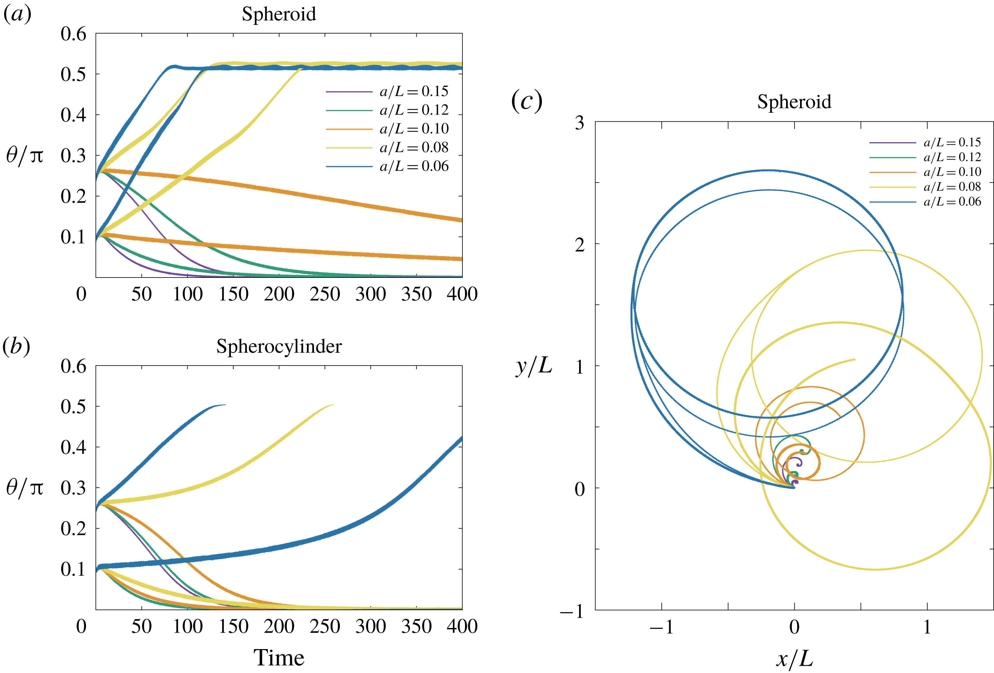
In figure 11(a,b), the time evolution of the inclination angle $\unicode[STIX]{x1D703}$ is plotted for the simulation of a pusher bacterial swimmer with different aspect ratios of the cell-body geometry. We have fixed the parameter values, $h/L=0.003$ , $\unicode[STIX]{x1D705}/\unicode[STIX]{x1D70F}=1$ and $c/L=0.15$ , while the dynamics for the different values of $a/L$ has been examined from $a/L=0.06$ (elongated shape) to $a/L=0.15$ (sphere). The corresponding trajectories of the cell-body centre are also shown for the spheroidal case (figure 11 c). These sets of the parameter values correspond to the stable upright spinning motion for a spherical cell body, but the spinning dynamics is found to be destabilized as the cell body becomes elongated in both cases of a spheroid and a spherocylinder. From figure 11(c), we have found the spherocylindrical cell body slightly enhances the upright motion rather than the spheroidal case. The spherocylinder simulation, however, has been terminated before the inclination angle exceeds the value of $\unicode[STIX]{x1D703}=\unicode[STIX]{x03C0}/2$ , because the problem becomes discontinuous at the configuration. When the flagellum is rotated backwards, the bacterial cell comes to an upright spinning position even for the elongated cell geometry (figure not shown), emphasizing the robust upright spinning dynamics for a puller flagellum in contrast to the pusher flagellar case, where the stable upright motion can be realized only in a limited range of parameter values.

5.1 Repulsive boundary

We start by considering that the wall boundary is purely repulsive in the vicinity of the boundary, and this situation can be achieved by neglecting adhesion effects, $k=0$ . From (2.14), the wall repulsion can be characterized by two parameters, the force strength $g$ , and the force length scale $\unicode[STIX]{x1D706}$ . With non-dimensionalizing these parameters using the units described in § 2.4, we have the dimensionless force strength, $F_{a}=gT/\unicode[STIX]{x1D707}$ , and inverse dimensionless length scale, $F_{b}=L/\unicode[STIX]{x1D706}$ . We consider a short-range strong repulsion, and we set $F_{a}=100$ since the force strength does not affect the swimmer behaviour if the value is sufficiently large (Ishimoto & Gaffney Reference Ishimoto and Gaffney2016). However, as seen in § 4.1, the force length scale, $F_{b}$ , determines the separation distance, and the bacterial dynamics with different length scales $F_{b}$ has been examined.

Figure 12.

Time evolution of the cell-body inclination angle $\unicode[STIX]{x1D703}$ and the flagellar bending angle $\unicode[STIX]{x1D711}$ in the free-swimming simulations of a model bacterium with different length scales of the wall repulsive force. The shape of the cell body is (a) a sphere of radius $a/L=c/L=0.15$ , (b) a spheroid of axis lengths $(a/L,c/L)=(0.1,0.15)$ , and (c) a spherocylinder of axis lengths $(a/L,c/L)=(0.1,0.15)$ . The inverse length scale of the wall force is varied within the range of $L/\unicode[STIX]{x1D706}=F_{b}=\{100,200,300,500\}$ , whereas constant values are used for the non-dimensional motor torque (0.03), hook rigidity $\unicode[STIX]{x1D705}/\unicode[STIX]{x1D70F}=1$ , and non-dimensional strength of the wall repulsion $F_{a}=100$ . The initial position of the cell-body centre is $H/L=0.3$ and the initial inclination angle is $\unicode[STIX]{x1D703}_{init}=0.25\unicode[STIX]{x03C0}$ .

In figure 12, we have plotted the time evolutions of the inclination and bending angles for the cell body of spherical, spheroidal and spherocylindrical geometries. The axes of the cell body are given by $c/L=0.1$ for a sphere and $c/L=0.15$ for a spheroid and spherocylinder, using the same minor axis of $a/L=0.1$ . The numerical simulations have been performed with different $F_{b}$ but with the same initial angle $\unicode[STIX]{x1D703}_{init}=0.25\unicode[STIX]{x03C0}$ and initial position $H/L=0.3$ . The hook rigidity is fixed as $\unicode[STIX]{x1D705}/\unicode[STIX]{x1D70F}=1$ and a pusher flagellum has been considered. We will compare the dynamics between free swimming with a repulsive wall and confined swimming with a constant separation distance in the previous sections.

Until the cell body reaches the region in the vicinity of the boundary (non-dimensional time of 20–40), the cell body slightly changes the inclination angle to follow the boundary, and this is purely due to hydrodynamic interactions (Shum et al. Reference Shum, Gaffney and Smith2010; Ishimoto & Gaffney Reference Ishimoto and Gaffney2017). Once the cell body experiences the repulsive force, the bacterial cell begins to stand upright, accompanied by the sudden increase of the bending angle, $\unicode[STIX]{x1D711}$ . If the force length scale is sufficiently small (large $F_{b}$ ), due to the torque by the misalignment between the cell body and flagellar orientations, the bacterial cell finally reaches the upright position, as seen in the confined swimming of § 4.

In the simulations with a spherical cell body (figure 12 a) and a short force length scale $\unicode[STIX]{x1D706}$ , the separation distance immediately converges to constant values, which reflects the force length scale. Thus the upright motion can be understood similarly to the confined swimming. However, in the case with the longer length scale of the force repulsion, the lubrication interactions are not sufficiently strong to sustain the cell body in a certain position and the cell finally follows the boundary ( $\unicode[STIX]{x1D703}=\unicode[STIX]{x03C0}/2$ ) with a considerably larger separation distance ( $H/L\approx 0.15$ ) than that which the repulsive force can affect ( $H/L\lesssim 0.11$ ). In this case, the boundary-following motion is stabilized purely by the hydrodynamic interactions as in the rigid hook case (Ishimoto & Gaffney Reference Ishimoto and Gaffney2017).

The similar swimming behaviours are found in the spheroidal and spherocylindrical cases with large $F_{b}$ values, where the cell body gradually orients towards the vertical configuration due to the torque generated by the misalignment between the cell body and flagellar orientations (figure 12 b,c). However, in the small $F_{b}$ case, the cell body is still oriented towards the boundary after a long time with nearly constant non-zero bending angles. This particular swimming dynamics can be characterized by a wall-following motion with continuous contacts to the boundary, and such a behaviour has been experimentally observed in P. aeruginosa bacterium and referred to as a horizontal spinning movement (de Anda et al. Reference de Anda, Lee, Lee, Bennet, Ji, Soltani, Harrison, Baker, Luo and Chou2017).

5.2 Adhesive boundary

We then proceed to the free-swimming bacterial dynamics near an adhesive boundary to investigate the complex nature of the bacterial spinning top observed in a P. aeruginosa bacterial cell. We consider spring bonds between the cell body and the boundary, motivated by the nano-spring property of the pili adhesion (Beaussart et al. Reference Beaussart, Baker, Kuchma, El-Kirat-Chatel, O’Toole and Dufren̂e2014).

Figure 13.

Time evolution of the cell-body inclination angle $\unicode[STIX]{x1D703}$ and the flagellar bending angle $\unicode[STIX]{x1D711}$ in the simulations with adhesive boundary. The shape of the cell body is (a) a sphere of radius $a/L=c/L=0.1$ , (b) a spheroid of axis lengths $(a/L,c/L)=(0.1,0.15)$ , and (c) a spherocylinder of axis lengths $(a/L,c/L)=(0.1,0.15)$ . The colours of the plots show the simulations with different values of hook rigidity $\unicode[STIX]{x1D705}/\unicode[STIX]{x1D70F}=\{10,1,0.1\}$ and adhesion strength $K=\{10^{3},10^{5}\}$ . Constant values are used for the non-dimensional motor torque (0.03) and non-dimensional length scale and strength scale of the wall repulsion ( $100$ and $300$ , respectively). The initial conditions are the same as in figure 12.

The strength of the adhesion is characterized by the spring constant $k$ of the bond, and we use dimensionless values for the adhesion strength, defined as $K=kLT/\unicode[STIX]{x1D707}$ . Other parameters regarding the creation and annihilation of adhesive bonds are given by $R_{ad}/L=0.01$ , $R_{on}/L=0.0101$ and $R_{off}/L=0.11$ , following the previous studies (Simons et al. Reference Simons, Olson, Cortez and Fauci2014; Ishimoto & Gaffney Reference Ishimoto and Gaffney2016). We also fix the values of the repulsive boundary force to be constant, $(F_{a},F_{b})=(100,300)$ .

In figure 13, the angle behaviours for the three different geometries of the cell body are shown as in § 5.1. We have examined bacterial dynamics with different values of hook rigidity $\unicode[STIX]{x1D705}/\unicode[STIX]{x1D70F}=\{10,1,0.1\}$ and adhesion strength $K=\{10^{3},10^{5}\}$ .

With a spherical cell body, the bacterium has been stuck to the boundary, except for the case of $(\unicode[STIX]{x1D705}/\unicode[STIX]{x1D70F},K)=(10,10^{3})$ , where the cell has exhibited a boundary-following motion (figure 13 a). Remarkably, the strong adhesion ( $K=10^{5}$ ) enabled the cell to stand upright even with the rigid hook parameter ( $\unicode[STIX]{x1D705}/\unicode[STIX]{x1D70F}=10$ ). Note that the upright motion was not possible without adhesive interactions. With a flexible hook ( $\unicode[STIX]{x1D705}/\unicode[STIX]{x1D70F}=0.1$ ), the inclination and bending angles have converged to non-trivial values, and the cell has exhibited a top-like spinning motion around a certain perpendicular axis. To express this motion visually, we have traced two points on the cell body: one corresponds to the flagellar connection point, and the other is the opposite point with respect to the cell-body centre, following the presentations in de Anda et al. (Reference de Anda, Lee, Lee, Bennet, Ji, Soltani, Harrison, Baker, Luo and Chou2017) for comparison. The time evolutions of these points are shown in colour in figure 14(a).

In the spheroidal and spherocylindrical simulations (figure 13 b,c,e,f), the cell body has eventually adhered to the boundary except for the cases with a rigid hook and weak adhesion value. The slight changes of the geometry have induced more complex behaviours such as non-steady behaviour with oscillatory angles, which emerge by the creation and annihilation of adhesive bonds. Example cell-body dynamics are shown in figure 14(b–d) for illustrations. In particular, with strong adhesion and flexible hook parameters, the angle values temporarily oscillate in an irregular manner, and the cell-body orbits become more complicated. Note that such unsteady dynamics of the bacterium have not been found in the simulations without adhesive interactions. Small differences of the aspect ratio are also found to generate further complex behaviours, as shown for the spheroidal cell-body case with $(a/L,c/L)=(0.075,0.15)$ in figure 14(d). These results suggest the rich diversity of the bacterial behaviour near an adhesive boundary, and the flexibility of the hook is found to be essential for the unsteady orbits.

Figure 14.

Example dynamics of the positions of the two pole ends of the cell body with different parameter values of adhesive strength, hook rigidity and cell-body geometry. The non-dimensional time is shown by the changes in colour. The constant parameters of the simulations are inherited from figure 13. The geometry of the cell body is (a) a sphere $a/L=c/L=0.1$ , (b) a spheroid of axis lengths $(a/L,c/L)=(0.1,0.15)$ , (c) a spherocylinder of axis lengths $(a/L,c/L)=(0.1,0.15)$ , and (d) a spheroid of axis lengths $(a/L,c/L)=(0.075,0.15)$ .