1 Introduction
Hovering is a distinct mode of locomotion in which a body subjected to gravity stays aloft with little or no average movement relative to a fixed point in space (Childress, Vandenberghe & Zhang Reference Childress, Vandenberghe and Zhang2006). Lift and stability are the two essential elements for achieving hovering flight.
Flying animals and some man-made flying vehicles utilize actuated wing motions to generate lift during hovering. Helicopters and rotary wing micro-air-vehicles (MAVs) rely on constant rotation of the rotor blades for lift generation (Hassanalian & Abdelkefi Reference Hassanalian and Abdelkefi2017). Insects, birds and ornithopters generate lift by the reciprocating motion of flapping wings (Weis-Fogh Reference Weis-Fogh1973; Norberg Reference Norberg1975; Wang Reference Wang2004). For these flapping-powered flyers, the delayed stall via leading-edge vortices (LEVs) is the dominant aerodynamic mechanism responsible for lift generation (Ellington et al. Reference Ellington, Berg, Willmott and Thomas1996; Dickinson & Sane Reference Dickinson, Lehmannand and Sane1999; Ramamurti & Sandberg Reference Ramamurti and Sandberg2002; Sun & Tang Reference Sun and Tang2002; Sane Reference Sane2003; Fry & Dickinson Reference Fry, Dickinson and Sayamanand2005; Wang Reference Wang2005; Aono, Liang & Liu Reference Aono, Liang and Liu2008).
Owing to the intrinsic instability of body orientation in the hovering flights of insects and flapping-powered robotic flyers, feedback active control systems were equipped for keeping the upright posture (Sun & Xiong Reference Sun and Xiong2005; Taylor & Krapp Reference Taylor and Krapp2007; Faruque & Humbert Reference Faruque and Humbert2010; Ratti & Vachtsevanos Reference Ratti and Vachtsevanos2010; Ristroph et al. Reference Ristroph, Bergou, Ristroph, Coumes, Berman, Guckenheimer, Wang and Cohen2010, Reference Ristroph, Ristroph, Morozova, Bergou, Chang, Guckenheimer, Wang and Cohen2013; Ma et al. Reference Ma, Chirarattananon, Fuller and Wood2013). Recently, an alternative wing actuation strategy by mimicking the swimming motion of a jellyfish was proposed by Ristroph & Childress (Reference Ristroph and Childress2014). They built a man-made hovering machine that can maintain postural stability without active controls. Subsequently, simplified two-dimensional computational models have been developed to analyse the aerodynamics and flight dynamics of the jellyfish-like flyer (Fang et al. Reference Fang, Ho, Ristroph and Shelley2017; Zhang et al. Reference Zhang, He, Wang and Zhang2018).
In parallel with the investigations on active flyers, hovering problems were also studied in the context of passive bodies without internal actuation. In the experiments on a flexible paper-folded ‘bug’ (Childress et al.
Reference Childress, Vandenberghe and Zhang2006) and a rigid hollow pyramid (Weathers et al.
Reference Weathers, Folie, Liu, Childress and Zhang2010; Liu et al.
Reference Liu, Ristroph, Weathers, Childress and Zhang2012) that were placed in a vertically oscillating flow with zero mean stream, some unexpected phenomena have been revealed. Although the objects with concave-down configuration can be unstable in free falling, such a configuration was found be stable in the passive hovering of paper-folded ‘bugs’ (Childress et al.
Reference Childress, Vandenberghe and Zhang2006). Another counterintuitive finding was that the elevation of the centre of mass of a hovering pyramid can actually increase its postural stability (Liu et al.
Reference Liu, Ristroph, Weathers, Childress and Zhang2012). To elucidate the underlying physical principles that govern the hovering of passive bodies, some two-dimensional computational studies on a rigid
 $\unicode[STIX]{x039B}$
-shaped model have been conducted (Huang, Nitsche & Kanso Reference Huang, Nitsche and Kanso2015, Reference Huang, Nitsche and Kanso2016; Shao et al.
Reference Shao, Zhang, Yu and Lin2016). The unsteady aerodynamic mechanisms responsible for lift generation, the actuation efforts required for hovering, and also the postural stability after perturbations were explored.
In some of the aforementioned active and passive hovering problems, flexibility is an important intrinsic property of the flyer. During hovering flights, passive deformation (or passive angular oscillation in the case of the
 $\unicode[STIX]{x039B}$
-model with a torsion spring) can be produced as a result of the combined effects of flexibility, aerodynamic load and wing inertia. For active flyers, some previous results indicated that the flexibility of the wing can enhance the lift generation and power efficiency (Vanella et al.
Reference Vanella, Fitzgerald, Preidikman, Balaras and Balachandran2009; Yin & Luo Reference Yin and Luo2010; Kang & Shyy Reference Kang and Shyy2013; Ristroph & Childress Reference Ristroph and Childress2014). The influences of flexibility were also found to be essential in the hovering of passive bodies. In the experiments on paper-folded ‘bugs’ (Childress et al.
Reference Childress, Vandenberghe and Zhang2006), it was observed that higher driving amplitudes of the background flow were required for very stiff ones to hover (i.e. flexibility can reduce the aerodynamic efforts needed for hovering). In the experiments on the passive hovering of hollow pyramids (Weathers et al.
Reference Weathers, Folie, Liu, Childress and Zhang2010), comparisons were made between a rigid pyramid and a pyramid with partially flexible sidewalls. It was found that the rigid pyramids can hover more easily (in comparison with the flexible ones), if the actuation frequency exceeded a certain value. We believe that the role of flexibility in passive hovering needs to be investigated in depth so as to rationalize the contradictory findings reported in these works. Furthermore, whether flexibility can reduce or increase the postural stability in passive hovering is also largely unexplored, although it was conjectured that flexibility has played a critical role in the stable hovering of paper-folded ‘bugs’ (Childress et al.
Reference Childress, Vandenberghe and Zhang2006).
Motivated by the experimental works of Childress et al. (Reference Childress, Vandenberghe and Zhang2006) and Weathers et al. (Reference Weathers, Folie, Liu, Childress and Zhang2010), we consider a two-dimensional
 $\unicode[STIX]{x039B}$
-model with an elastic torsion spring installed at the hinged joint. We numerically solve the coupled Navier–Stokes equations and dynamic equations to explore the impacts of flexibility on the performance of passive hovering flight. There are several reasons for adopting a two-dimensional model rather than a three-dimensional one in the current study. First, the results obtained from the two-dimensional model can still shed light on the aerodynamics of a passive body driven by oscillating flow, although three-dimensional effects in the experiments are excluded. Second, the high computational cost in three-dimensional (3-D) simulation renders thorough parameter sweeps prohibitive. Third, we intend to make comparison between the results of the present study and those of other two-dimensional (2-D) systems (such as the pinned and rotatable
 $\unicode[STIX]{x039B}$
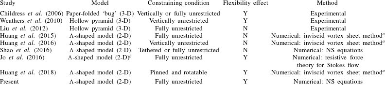
-flyer studied by Huang et al. (Reference Huang, Ristroph, Luhar and Kanso2018)). In table 1, we present a summary of the studies on the passive motion of an object driven by an oscillating flow. It is seen that, although the two-dimensional
 $\unicode[STIX]{x039B}$
-shaped model was adopted previously in some numerical studies, the flexibility effect on passive hovering performance has never been explored by using high-fidelity computational fluid dynamics simulations.
The rest of the paper is organized as follows. In § 2, we present the computational model and governing equations. The numerical methods and computational settings are introduced in § 3. In § 4, we explore the influences of some control parameters on passive flights, the actuation efforts required for hovering, the passive angular oscillation patterns, and the wake symmetry and postural stability properties. The main findings of the present study are summarized in § 5.
Summary of the studies on the passive motion of an object driven by an oscillatory flow.

a Simulations in these studies are based on the inviscid-flow model, although a dissipation time is introduced to imitate viscosity.
b The force of gravity is not included in the model (neutral buoyancy condition is assumed).
2 Problem description
2.1 Computational model
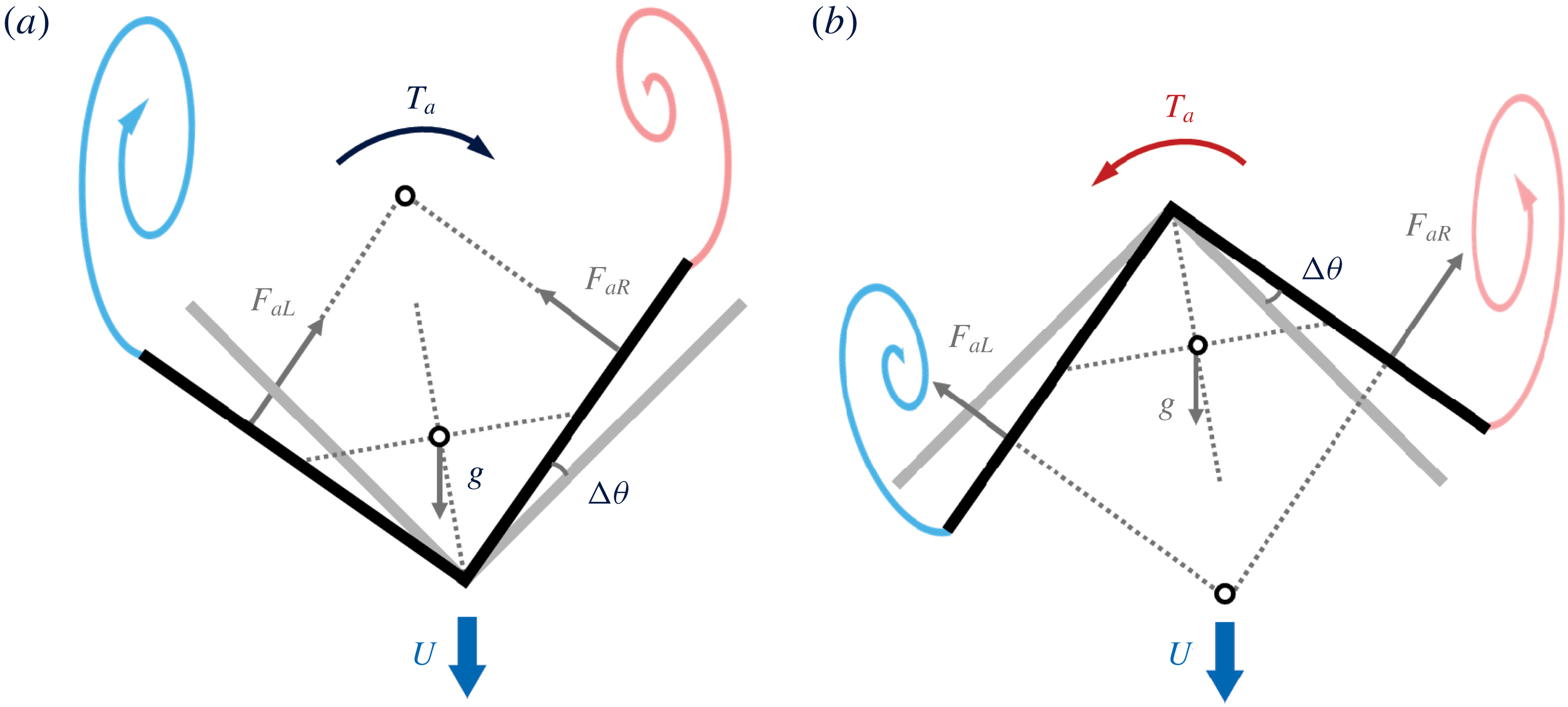
We consider a flexible
 $\unicode[STIX]{x039B}$
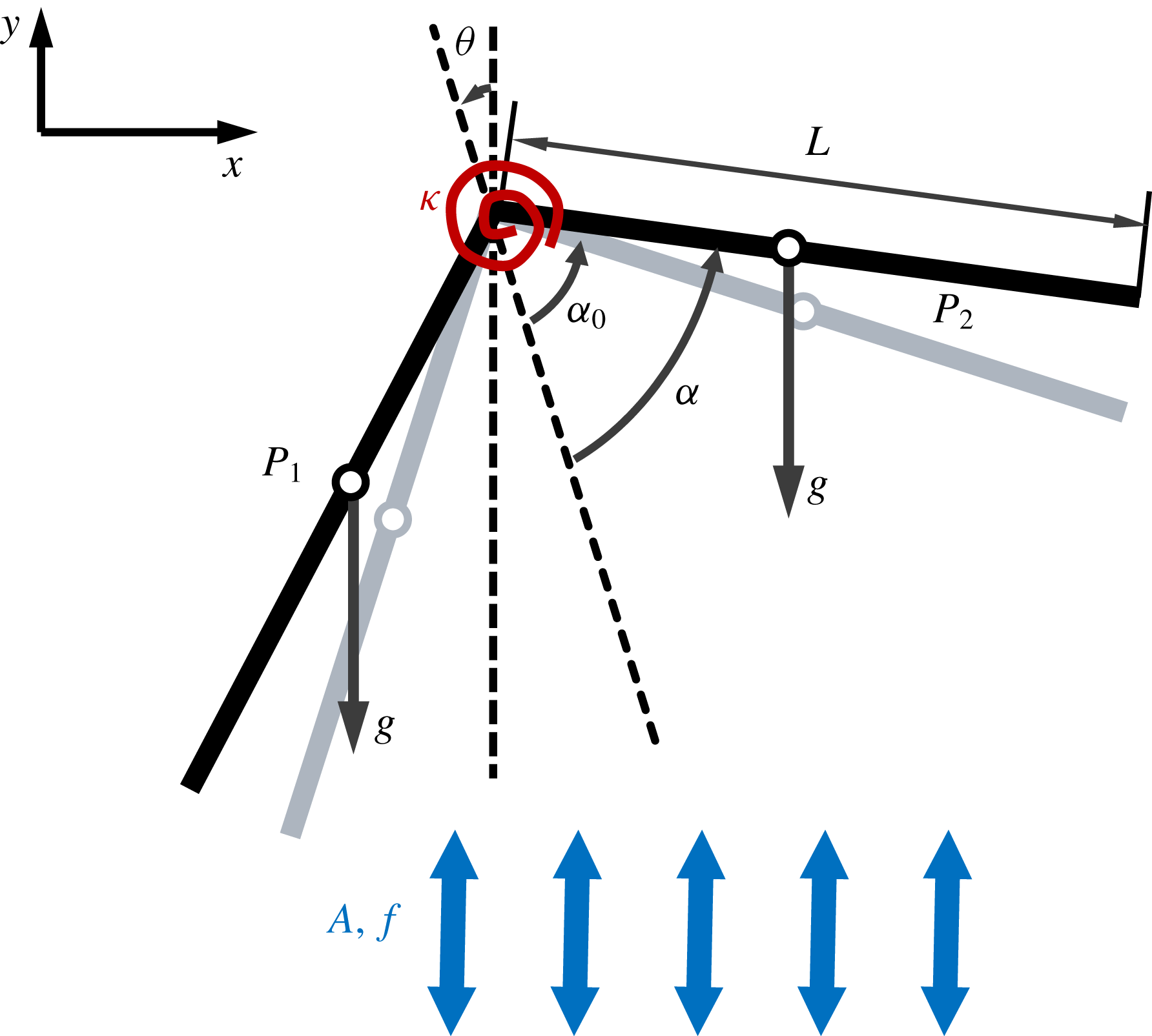
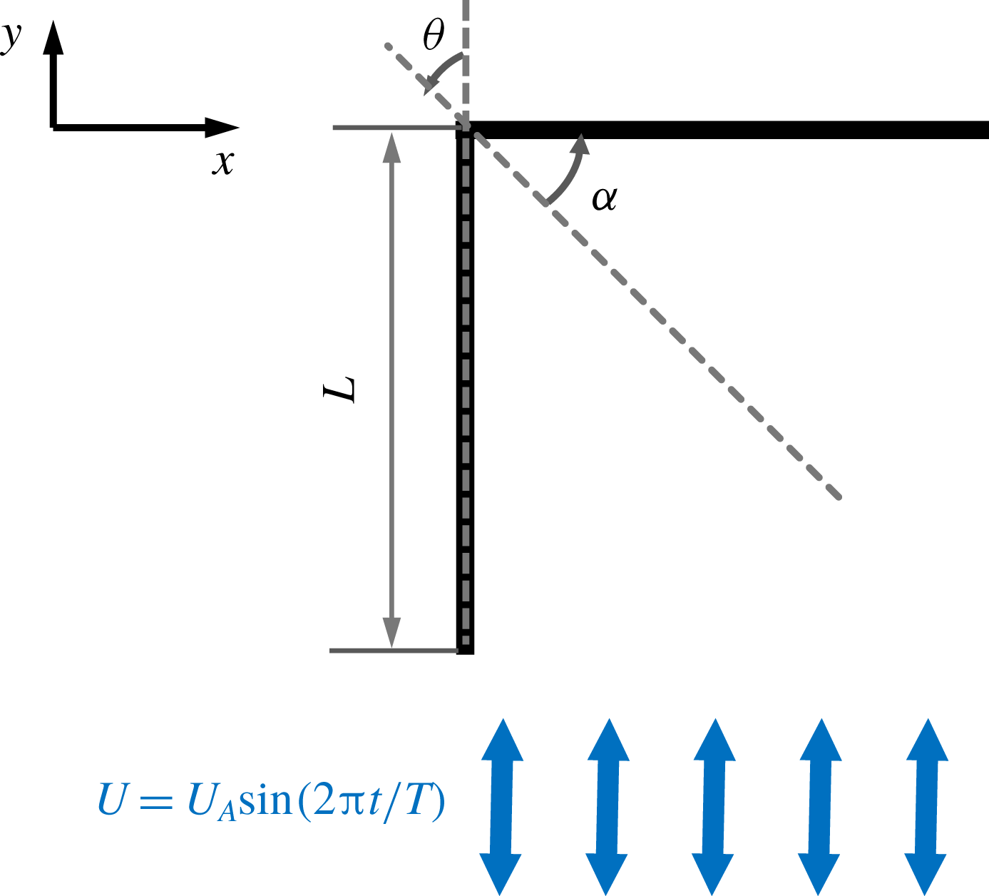
-flyer in a vertically oscillating flow, as shown in figure 1. The flyer consists of two rigid thin foils which are connected elastically at the hinged joint via a torsion spring. The vertical velocity of the imposed background flow is a sinusoidal function of time. The flyer is allowed to move freely in the oscillatory background flow, while the two foils can also flap passively as a result of the aerodynamic torques.
A schematic diagram of the computational model. Here
 $L$
is the chord length of the foils;
 $\unicode[STIX]{x1D6FC}$
and
 $\unicode[STIX]{x1D6FC}_{0}$
denote the opening angle and resting angle, respectively;
 $\unicode[STIX]{x1D703}$
is the inclination angle of the centreline with respect to the
 $y$
-axis;
 $P_{1}$
and
 $P_{2}$
denote the centres of gravity of the two foils;
 $g$
represents the acceleration due to gravity; and
 $A$
and
 $f$
are the amplitude and frequency of the imposed oscillatory flow, respectively.

The (dimensional) vertical velocity of the background flow is prescribed as
 $U_{y}(t^{\ast })=2\unicode[STIX]{x03C0}Af\sin (2\unicode[STIX]{x03C0}ft^{\ast })$
, where
 $A$
,
 $f$
and
 $t^{\ast }$
are the oscillating amplitude, the oscillating frequency and the (dimensional) time, respectively. Other control parameters of the system include: the stiffness of the torsional spring (
 $\unicode[STIX]{x1D705}$
), the densities of the flyer and the fluid (
 $\unicode[STIX]{x1D70C}_{s}$
and
 $\unicode[STIX]{x1D70C}_{f}$
), the chord length and thickness of the two foils (
 $L$
and
 $\unicode[STIX]{x1D6FF}$
), the kinematic viscosity of the fluid (
 $\unicode[STIX]{x1D708}$
) and the gravitational acceleration (
 $g$
). We select
 $L$
,
 $1/f$
and
 $\unicode[STIX]{x1D70C}_{f}$
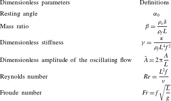
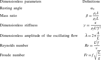
as the reference quantities for length, time and density to scale the system. The dimensionless control parameters of the system (including those that arise as a result of the scaling) are summarized in table 2.
Dimensionless parameters of the system.
The incompressible Navier–Stokes equations that govern the fluid motion can be written in dimensionless form as
 $$\begin{eqnarray}\displaystyle & \displaystyle \frac{\unicode[STIX]{x2202}\boldsymbol{u}}{\unicode[STIX]{x2202}t}+(\boldsymbol{u}\boldsymbol{\cdot }\unicode[STIX]{x1D735})\boldsymbol{u}=-\unicode[STIX]{x1D735}p^{\prime }+\frac{1}{Re}\unicode[STIX]{x1D6FB}^{2}\,\boldsymbol{u}+\boldsymbol{f}, & \displaystyle\end{eqnarray}$$
 $$\begin{eqnarray}\displaystyle & \displaystyle \unicode[STIX]{x1D735}\boldsymbol{\cdot }\boldsymbol{u}=0, & \displaystyle\end{eqnarray}$$
 $\boldsymbol{u}$
is the fluid velocity vector,
 $p^{\prime }$
is the modified pressure, which absorbs the hydrostatic pressure due to the force of gravity, and
 $\boldsymbol{f}$
is the Eulerian forcing term, which represents the effect of an immersed object on the flow.
The dimensionless dynamic equations that govern the motion of the flyer can be written as
 $$\begin{eqnarray}\unicode[STIX]{x1D648}\ddot{\boldsymbol{q}}=\boldsymbol{F}_{i}+\boldsymbol{F}_{k}+\boldsymbol{F}_{g}+\boldsymbol{F}_{a},\end{eqnarray}$$
where
 $\unicode[STIX]{x1D648}$
is the mass matrix and
 $\boldsymbol{q}=[x,y,\unicode[STIX]{x1D703}-\unicode[STIX]{x1D6FC},\unicode[STIX]{x1D703}+\unicode[STIX]{x1D6FC}]^{\text{T}}$
is the generalized displacement vector for the translational and rotational motions. Here
 $x$
and
 $y$
denote the horizontal and vertical displacements of the apex, respectively; and
 $(\unicode[STIX]{x1D703}-\unicode[STIX]{x1D6FC})$
and
 $(\unicode[STIX]{x1D703}+\unicode[STIX]{x1D6FC})$
are the inclination angles of the two foils with respect to the
 $y$
-axis, respectively. The double dot represents the second derivative with respect to time. The four vectors on the right-hand side of (2.2) are the inertial, elastic, gravitational and aerodynamic forces (and torques), respectively. Since the density of the air is much lower than that of the flyer and the volume occupied by the flyer is negligibly small, the buoyancy force and torque are not included in (2.2).
The mass matrix
 $\unicode[STIX]{x1D648}$
in (2.2) is given by
 $$\begin{eqnarray}\unicode[STIX]{x1D648}=\left[\begin{array}{@{}cccc@{}}2\unicode[STIX]{x1D6FD} & 0 & \unicode[STIX]{x1D6FD}l_{c}\cos (\unicode[STIX]{x1D703}-\unicode[STIX]{x1D6FC}) & \unicode[STIX]{x1D6FD}l_{c}\cos (\unicode[STIX]{x1D703}+\unicode[STIX]{x1D6FC})\\ 0 & 2\unicode[STIX]{x1D6FD} & \unicode[STIX]{x1D6FD}l_{c}\sin (\unicode[STIX]{x1D703}-\unicode[STIX]{x1D6FC}) & \unicode[STIX]{x1D6FD}l_{c}\sin (\unicode[STIX]{x1D703}+\unicode[STIX]{x1D6FC})\\ \unicode[STIX]{x1D6FD}l_{c}\cos (\unicode[STIX]{x1D703}-\unicode[STIX]{x1D6FC}) & \unicode[STIX]{x1D6FD}l_{c}\sin (\unicode[STIX]{x1D703}-\unicode[STIX]{x1D6FC}) & J & 0\\ \unicode[STIX]{x1D6FD}l_{c}\cos (\unicode[STIX]{x1D703}+\unicode[STIX]{x1D6FC}) & \unicode[STIX]{x1D6FD}l_{c}\sin (\unicode[STIX]{x1D703}+\unicode[STIX]{x1D6FC}) & 0 & J\end{array}\right],\end{eqnarray}$$
where
 $l_{c}$
is the (dimensionless) distance between the centre of gravity of each foil and the apex, and
 $J$
is the dimensionless moment of inertia of each foil with respect to the apex. For a flyer with homogeneous density,
 $l_{c}=1/2$
and
 $J=\unicode[STIX]{x1D6FD}/3$
.
The inertial, elastic and gravitational forces (and torques) are given by
 $$\begin{eqnarray}\displaystyle & \displaystyle \boldsymbol{F}_{i}=\left[\begin{array}{@{}c@{}}\unicode[STIX]{x1D6FD}l_{c}[\sin (\unicode[STIX]{x1D703}-\unicode[STIX]{x1D6FC})(\dot{\unicode[STIX]{x1D703}}-\dot{\unicode[STIX]{x1D6FC}})^{2}+\sin (\unicode[STIX]{x1D703}+\unicode[STIX]{x1D6FC})(\dot{\unicode[STIX]{x1D703}}+\dot{\unicode[STIX]{x1D6FC}})^{2}]\\ -\unicode[STIX]{x1D6FD}l_{c}[\cos (\unicode[STIX]{x1D703}-\unicode[STIX]{x1D6FC})(\dot{\unicode[STIX]{x1D703}}-\dot{\unicode[STIX]{x1D6FC}})^{2}+\cos (\unicode[STIX]{x1D703}+\unicode[STIX]{x1D6FC})(\dot{\unicode[STIX]{x1D703}}+\dot{\unicode[STIX]{x1D6FC}})^{2}]\\ 0\\ 0\end{array}\right], & \displaystyle\end{eqnarray}$$
 $$\begin{eqnarray}\displaystyle & \displaystyle \boldsymbol{F}_{k}=\left[\begin{array}{@{}c@{}}0\\ 0\\ \unicode[STIX]{x1D6FE}(\unicode[STIX]{x1D6FC}-\unicode[STIX]{x1D6FC}_{0})\\ -\unicode[STIX]{x1D6FE}(\unicode[STIX]{x1D6FC}-\unicode[STIX]{x1D6FC}_{0})\end{array}\right], & \displaystyle\end{eqnarray}$$
 $$\begin{eqnarray}\displaystyle & \displaystyle \boldsymbol{F}_{g}=\left[\begin{array}{@{}c@{}}0\\ -2\unicode[STIX]{x1D6FD}/Fr^{2}\\ -\unicode[STIX]{x1D6FD}(l_{c}/Fr^{2})\sin (\unicode[STIX]{x1D703}-\unicode[STIX]{x1D6FC})\\ -\unicode[STIX]{x1D6FD}(l_{c}/Fr^{2})\sin (\unicode[STIX]{x1D703}+\unicode[STIX]{x1D6FC})\end{array}\right], & \displaystyle\end{eqnarray}$$
 $\unicode[STIX]{x1D6FC}_{0}$
is the resting angle.
The aerodynamic forces (and torques) are given by
 $$\begin{eqnarray}\boldsymbol{F}_{a}=[F_{a1},F_{a2},F_{a3},F_{a4}]^{\text{T}}=\left[\begin{array}{@{}c@{}}\displaystyle \mathop{\sum }_{i}[\boldsymbol{F}(\boldsymbol{X}_{i})\boldsymbol{\cdot }\boldsymbol{i}]\unicode[STIX]{x0394}s\\ \displaystyle \mathop{\sum }_{i}[\boldsymbol{F}(\boldsymbol{X}_{i})\boldsymbol{\cdot }\boldsymbol{j}]\unicode[STIX]{x0394}s\\ \displaystyle \mathop{\sum }_{i}^{L}[(\boldsymbol{X}_{i}-\boldsymbol{X}_{a})\times \boldsymbol{F}(\boldsymbol{X}_{i})\boldsymbol{\cdot }\boldsymbol{k}]\unicode[STIX]{x0394}s\\ \displaystyle \mathop{\sum }_{i}^{R}[(\boldsymbol{X}_{i}-\boldsymbol{X}_{a})\times \boldsymbol{F}(\boldsymbol{X}_{i})\boldsymbol{\cdot }\boldsymbol{k}]\unicode[STIX]{x0394}s\end{array}\right],\end{eqnarray}$$
where
 $\boldsymbol{X}_{i}$
and
 $\boldsymbol{X}_{a}$
are the position vectors of the Lagrangian point and the apex, respectively;
 $\boldsymbol{i}$
and
 $\boldsymbol{j}$
are the unit vectors along the
 $x$
-axis and
 $y$
-axis, respectively;
 $\boldsymbol{k}$
is the unit vector that points outwards from the
 $x{-}y$
plane;
 $\boldsymbol{F}$
is the Lagrangian forcing term, which represents the interaction between the flyer and the surrounding fluid; and
 $\unicode[STIX]{x0394}s$
is the width of the Lagrangian grid. The symbols ‘
 $L$
’ and ‘
 $R$
’ above the summation symbol denote the left and the right foils, respectively.
The system of dynamic equations (2.2) is similar to the one used by Jo et al. (Reference Jo, Huang, Zimmermann and Kanso2016), where the passive locomotion of a flexible
 $\unicode[STIX]{x039B}$
-model in an oscillatory Stokes flow was studied. There are only two differences between the two systems. First, the gravitational force and torque are not included in Jo et al. (Reference Jo, Huang, Zimmermann and Kanso2016) since the model is neutrally buoyant. Second, the expressions for the fluid force and torque are different. In the case when linear displacements are not permitted, equation (2.2) degenerates into the system of dynamic equations for describing the behaviours of a pinned and rotatable flexible
 $\unicode[STIX]{x039B}$
-flyer (Huang et al.
Reference Huang, Ristroph, Luhar and Kanso2018).
3 Numerical methods and computational settings
3.1 Flow and dynamics solvers
The Navier–Stokes equations are solved by using the direct-forcing immersed boundary method based on the discrete streamfunction formulation (Wang & Zhang Reference Wang and Zhang2011). The flow solver is parallelized by using the message passing interface (MPI) protocol (Wang, He & Zhang Reference Wang, He and Zhang2013). The finite difference method is used to discretize the dynamic equations, and the explicit Eulerian scheme is used for the temporal advancement. A loosely coupled scheme, in which the fluid equations and dynamic equations are advanced sequentially, is used to conduct the flow–structure interaction simulations.
The code used here has been validated thoroughly in previous studies by using a variety of numerical examples, such as flows over stationary objects and objects with prescribed motions (Wang & Zhang Reference Wang and Zhang2011; Wang et al.
Reference Wang, He and Zhang2013), and the self-propelled swimming of elastic filaments (Zhu, He & Zhang Reference Zhu, He and Zhang2014a
,Reference Zhu, He and Zhang
b
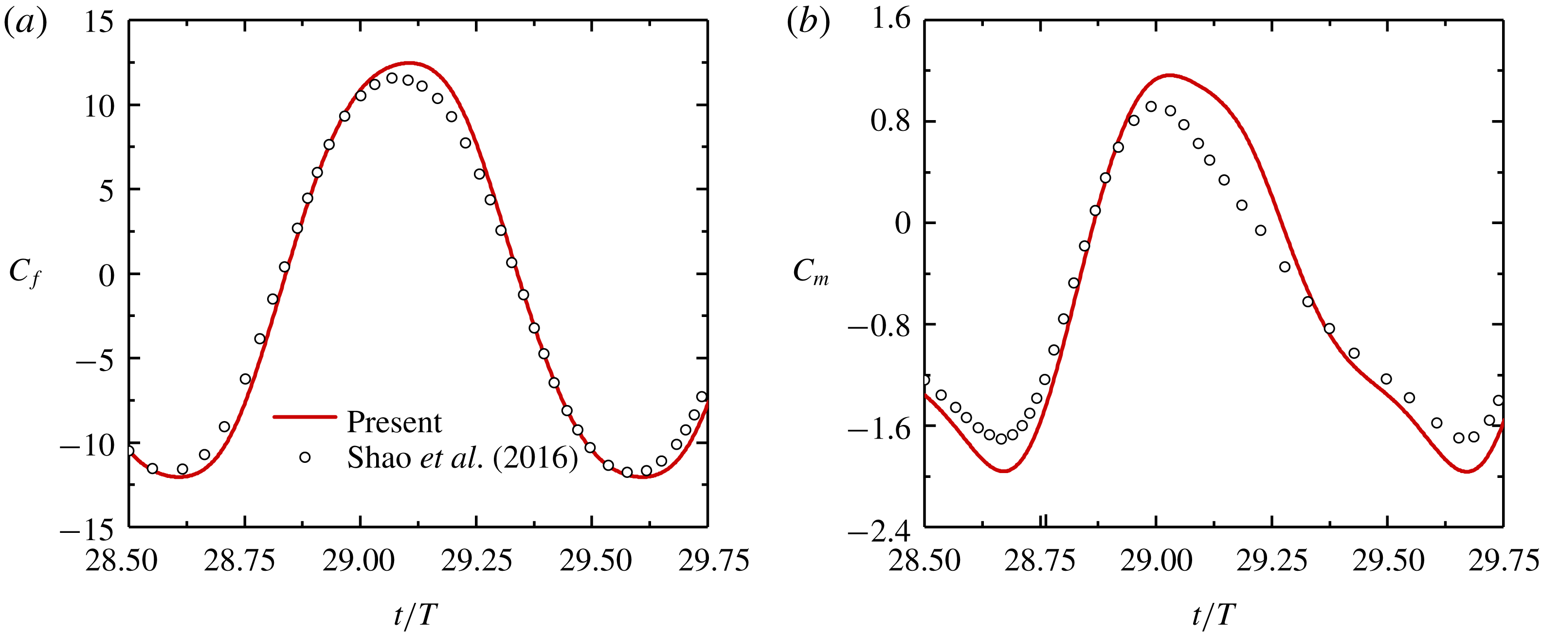
). In addition to the examples mentioned above, another validation is also conducted by computing the aerodynamic force and moment on a rigid
 $\unicode[STIX]{x039B}$
-model fixed in an oscillating flow (Shao et al.
Reference Shao, Zhang, Yu and Lin2016). A good match between the results of these two works is shown in appendix A.
3.2 Boundary and initial conditions
Since the streamfunction is used as the primary unknown in the flow solver, both the streamfunction
 $s$
and the tangential velocity need to be specified on the boundaries. The computational domain is rectangular in shape and has a width of
 $2W$
. On the left boundary, the streamfunction is set to zero (i.e.
 $s(-W/L,y,t)=0$
). On the right boundary, the streamfunction is set to a sinusoidal function of time. This function is obtained by converting the imposed volumetric flow rate between the left and right boundaries (i.e.
 $s(W/L,y,t)=-(2W/L)\bar{A}\sin (2\unicode[STIX]{x03C0}t)$
). On the top and bottom boundaries, the inflow/outflow conditions are implemented by allowing the boundary streamfunction to be treated as an unknown (Wang, Francis & Perot Reference Wang, Francis and Perot2002). Moreover, the normal derivative of the tangential velocity is set to zero on all four boundaries. Since
 $\unicode[STIX]{x1D6FF}\ll L$
, the two links of the flyer are modelled as two flat plates that have ‘zero’ thickness nominally. In the two-dimensional simulation, the two flat plates are represented by
 $101$
Lagrangian points each and the non-slip boundary condition is enforced on these points by using the direct-forcing immersed boundary technique (Wang & Zhang Reference Wang and Zhang2011).
The initial velocities for both the fluid and the
 $\unicode[STIX]{x039B}$
-flyer are set to zero. For the investigations on the influences of some control parameters on passive flights, the actuation efforts needed for hovering, the angular oscillation patterns and the wake symmetry properties (§§ 4.2–4.5), both the initial inclination angle
 $\unicode[STIX]{x1D703}(0)$
and the initial rotational speed
 $\dot{\unicode[STIX]{x1D703}}(0)$
are set to zero. For the investigation on the postural stability behaviours (§ 4.6), non-zero initial inclination angles are considered, i.e.
 $\unicode[STIX]{x1D703}(0)\neq 0$
, while the condition
 $\dot{\unicode[STIX]{x1D703}}(0)=0$
is still kept. For all cases in the simulations,
 $\unicode[STIX]{x1D6FC}(0)=\unicode[STIX]{x1D6FC}_{0}$
and
 $\dot{\unicode[STIX]{x1D6FC}}(0)=0$
are used as the initial conditions for the passive angular oscillation.
3.3 Domain size and mesh resolution
For the simulations with zero initial inclination angles (§§ 4.2–4.5), a rectangular domain of
 $[-6L,6L]\times [-12L,12L]$
is used. For the study of the postural stability behaviours (§ 4.6), an enlarged computational domain of
 $[-10L,10L]\times [-16L,16L]$
is used to cope with possible large lateral displacements.
Multi-block Cartesian meshes with hanging nodes are employed in this work. The meshes remain stationary throughout the simulation and the flyer is allowed to move freely in the computational domain. The grid width ranges from
 $0.02L$
to
 $0.04L$
in regions that are far away from the flyer. In the vicinity of the flyer, the grid width is reduced to
 $0.01L$
for capturing the relevant flow structures. For the domain size of
 $[-6L,6L]\times [-12L,12L]$
, the refined grids are deployed in the subdomain of
 $[-2L,2L]\times [-8L,8L]$
. For the domain size of
 $[-10L,10L]\times [-16L,16L]$
, the subdomain with refined grids is enlarged to
 $[-8L,8L]\times [-8L,8L]$
. For all simulation cases, the time steps are chosen such that the maximum Courant–Friedrichs–Lewy (CFL) number never exceeds
 $0.2$
.
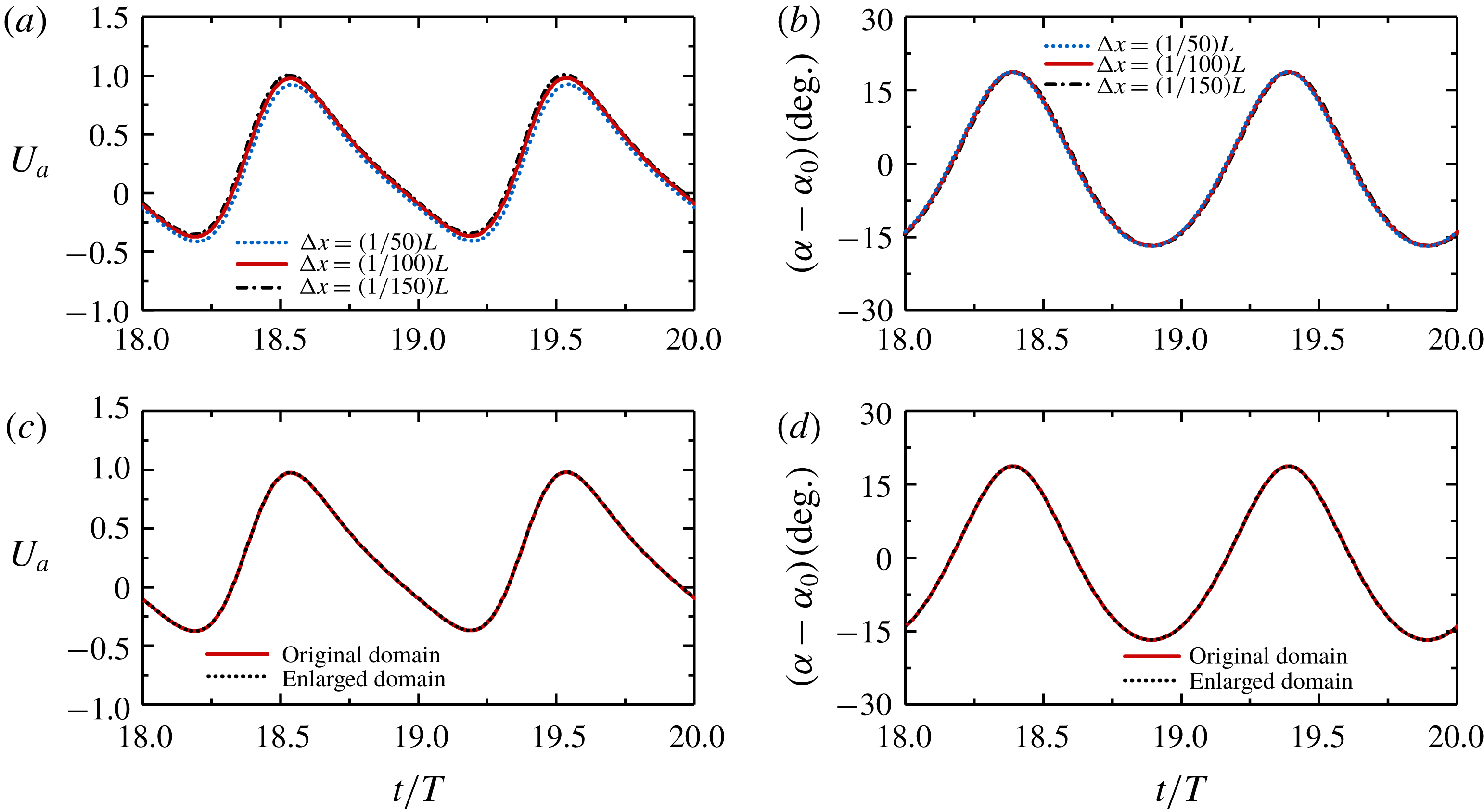
To ensure that the aforementioned mesh resolution and domain size are suitable for obtaining accurate solutions, mesh independence and domain independence tests have been conducted. A report of the tests is presented in appendix B.
4 Results and discussion
4.1 Control parameters
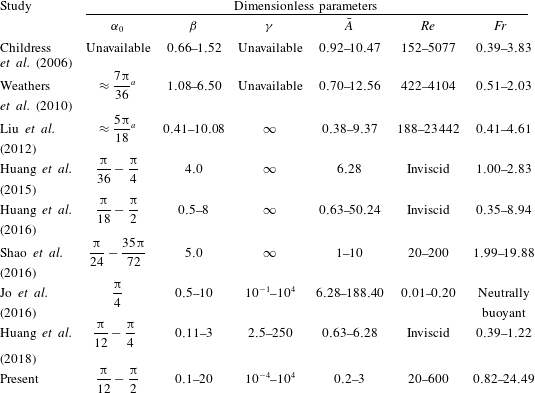
The ranges of the dimensionless parameters used in the present study and some previous studies are listed in table 3. The maximum
 $Re$
number considered in the current study is one or two orders of magnitude smaller, in comparison with those in the experiments (Childress et al.
Reference Childress, Vandenberghe and Zhang2006; Weathers et al.
Reference Weathers, Folie, Liu, Childress and Zhang2010; Liu et al.
Reference Liu, Ristroph, Weathers, Childress and Zhang2012). The reason for reducing the
 $Re$
number in the simulation is related to the computational cost. Simulation at
 $Re$
numbers comparable to those in the experiments requires much higher mesh resolution. This may render thorough parameter sweeps prohibitive.
The dimensionless maximum oscillation amplitude in the simulation is reduced by a factor of 3–4, in comparison with those in the experiments. The reason for reducing the oscillation amplitude is very similar to that for reducing the
 $Re$
number. Here we are concerned with another Reynolds number, namely, the oscillating Reynolds number, which is defined as
 $Re_{o}=2\unicode[STIX]{x03C0}fAL/\unicode[STIX]{x1D708}$
(in which the maximum oscillating speed of the background flow is selected as the reference velocity). The oscillating Reynolds number
 $Re_{o}$
is related to
 $Re$
by
 $Re_{o}=\bar{A}\,Re$
. The reduction of
 $\bar{A}$
results in lower
 $Re_{o}$
and makes the simulation feasible.
The ranges for
 $Re$
and
 $\bar{A}$
in the current study are selected such that the two Reynolds numbers (
 $Re$
and
 $Re_{o}$
) are comparable to those in Shao et al. (Reference Shao, Zhang, Yu and Lin2016), since the Navier–Stokes equations were also solved in their study. The ranges for other parameters in the two studies are also close. The dimensionless stiffness is the only exception. In Shao et al. (Reference Shao, Zhang, Yu and Lin2016), the dimensionless stiffness can be regarded as infinitely large since only rigid flyers were considered.
The
 $Re$
-sensitivity tests in some previous studies on active flappers (e.g. Zhang et al.
Reference Zhang, He, Wang and Zhang2018) indicated that the flight performance may be insensitive to
 $Re$
in the range of
 $10^{2}{-}10^{3}$
. However, caution should be taken if one attempts to apply the present results to situations involving much larger
 $Re$
.
Summary of the dimensionless parameters used in the literature and in the present work.
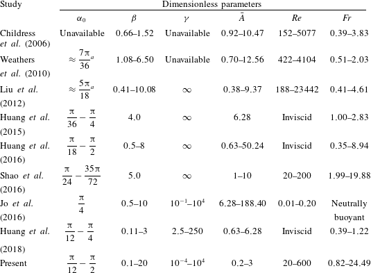
a The resting angle of the 3-D pyramid model is estimated by using the cross-section geometry.
4.2 Influences of spring stiffness, density and resting angle
In this section, the influences of some control parameters on the passive flights of a flyer with concave-down configuration are systematically studied. Specifically, we examine the influences of spring stiffness, density and resting angle, under a given actuation condition (where the driving frequency and amplitude are fixed). In terms of the dimensionless variables, the dimensionless stiffness
 $\unicode[STIX]{x1D6FE}$
, the mass ratio
 $\unicode[STIX]{x1D6FD}$
and the resting angle
 $\unicode[STIX]{x1D6FC}_{0}$
are allowed to vary, while the dimensionless amplitude
 $\bar{A}$
, the flapping Reynolds number
 $Re$
and the Froude number
 $Fr$
are fixed (
 $\bar{A}=1.0$
,
 $Re=200$
,
 $Fr=8.165$
). The selection of these particular values is based on the following considerations: (a)
 $Re$
and
 $\bar{A}$
are reduced to some extent in comparison with the values in the experiments (the reasons have been provided in § 4.1), and (b)
 $Fr$
is tuned such that the hovering state is achieved in the rigid flyer (
 $\unicode[STIX]{x1D6FE}=10^{4}$
) with
 $\unicode[STIX]{x1D6FD}=2.0$
and
 $\unicode[STIX]{x1D6FC}_{0}=45^{\circ }$
.
The important metrics for evaluating the flyer’s performance in passive flight include the averaged opening angle, the averaged vertical speed and the amplitudes of angular and vertical oscillations. These four metrics are formally defined as
 $$\begin{eqnarray}\displaystyle & \displaystyle \bar{\unicode[STIX]{x1D6FC}}=\frac{1}{nT}\int _{T_{0}}^{T_{0}+nT}\unicode[STIX]{x1D6FC}(t)\,\text{d}t, & \displaystyle\end{eqnarray}$$
 $$\begin{eqnarray}\displaystyle & \displaystyle \bar{U}=\frac{1}{nT}\int _{T_{0}}^{T_{0}+nT}{\dot{y}}_{a}(t)\,\text{d}t, & \displaystyle\end{eqnarray}$$
 $$\begin{eqnarray}\displaystyle & \displaystyle \bar{\unicode[STIX]{x1D6FC}}_{osc}=\frac{1}{n}\mathop{\sum }_{i=0}^{n-1}\left.\frac{1}{2}\{\max [\unicode[STIX]{x1D6FC}(t_{i})]-\min [\unicode[STIX]{x1D6FC}(t_{i})]\}\right|_{T_{0}+iT\leqslant t_{i}\leqslant T_{0}+(i+1)T}, & \displaystyle\end{eqnarray}$$
 $$\begin{eqnarray}\displaystyle & \displaystyle \bar{U}_{osc}=\frac{1}{n}\mathop{\sum }_{i=0}^{n-1}\left.\frac{1}{2}\{\max [{\dot{y}}_{a}(t_{i})]-\min [{\dot{y}}_{a}(t_{i})]\}\right|_{T_{0}+iT\leqslant t_{i}\leqslant T_{0}+(i+1)T}, & \displaystyle\end{eqnarray}$$
where
 $T_{0}$
is the starting time for the sampling,
 $n$
and
 $i$
are integers,
 $T$
is the dimensionless period of the imposed oscillatory flow (which equals unity) and
 ${\dot{y}}_{a}(t)$
is the instantaneous vertical speed of the apex.
The starting time
 $T_{0}$
is chosen such that the influence of initial condition becomes insignificant and the periodicity in the time histories is fully established (usually
 $T_{0}=20$
is considered to be sufficient). The integer
 $n$
is chosen to be
 $5$
, for the cases of mono-periodic and bi-periodic angular oscillations. For the cases of non-periodic oscillation, the averaged values and amplitudes of oscillation are loosely defined by setting
 $n=30$
. The locomotion states of the flyers can be classified as ‘ascending’ and ‘descending’, based on the sign of the averaged vertical speed. In addition, we also used the term ‘approximate hovering state’ when the absolute value of the averaged vertical speed is less than
 $0.05$
.
We first explore the influence of dimensionless stiffness. To this end,
 $\unicode[STIX]{x1D6FE}$
is allowed to vary in a wide range of
 $10^{-4}{-}10^{4}$
(due to the variation of
 $\unicode[STIX]{x1D705}$
), while the mass ratio and the resting angle are kept fixed (
 $\unicode[STIX]{x1D6FD}=2.0$
,
 $\unicode[STIX]{x1D6FC}_{0}=45^{\circ }$
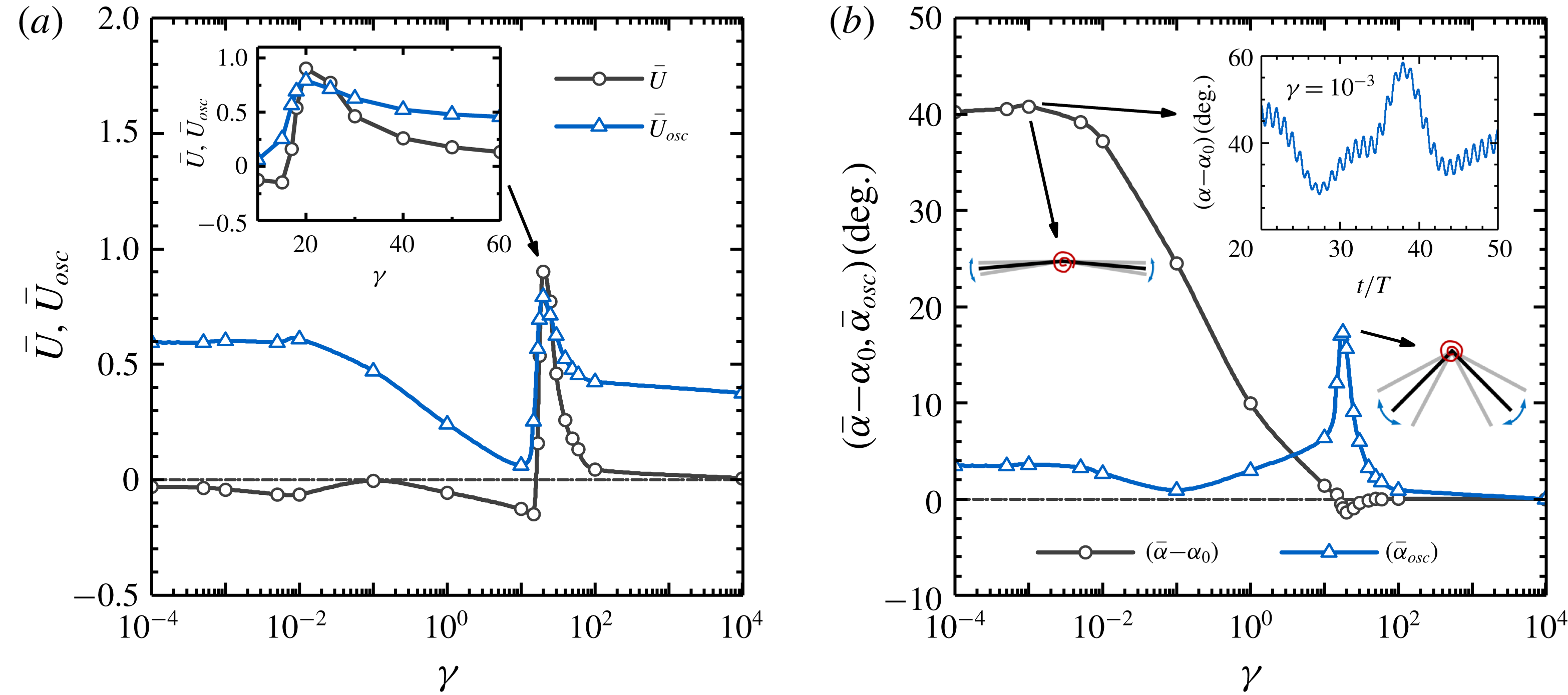
). Figure 2(a) shows the averaged vertical speed and the amplitude of vertical oscillation as a function of
 $\unicode[STIX]{x1D6FE}$
. It is seen that the softest flyer tends to descend gently, while a rigid flyer is able to sustain hovering approximately. A ‘pulse’ in the averaged vertical speed is observed at
 $\unicode[STIX]{x1D6FE}=30$
, where the peak value of 0.9 is achieved. The amplitudes of vertical oscillation are rather high at low stiffness (and take a value around 0.6 in the range of
 $10^{-4}<\unicode[STIX]{x1D6FE}<10^{-2}$
). The amplitude of vertical oscillation then decreases with increasing stiffness and reaches the minimal value of 0.05 at
 $\unicode[STIX]{x1D6FE}=10$
. At
 $\unicode[STIX]{x1D6FE}=30$
, where the ‘pulse’ in the averaged speed is observed, a ‘pulse’ in the amplitude of vertical oscillation is also found. The amplitude of vertical oscillation declines rapidly in the range of
 $30<\unicode[STIX]{x1D6FE}<100$
and finally levels off and takes a value of 0.38 at extremely high stiffness.
Figure 2(b) shows the variations of averaged opening angle and amplitude of angular oscillation with increasing
 $\unicode[STIX]{x1D6FE}$
. It is seen that the averaged opening angle becomes much larger than the resting angle
 $\unicode[STIX]{x1D6FC}_{0}$
in very soft flyers (the increment can reach up to
 $40^{\circ }$
at
 $\unicode[STIX]{x1D6FE}=10^{-4}$
). The increment decreases monotonically with increasing
 $\unicode[STIX]{x1D6FE}$
in the range of
 $10^{-3}<\unicode[STIX]{x1D6FE}<15.0$
and approaches zero at
 $\unicode[STIX]{x1D6FE}\approx 15.0$
. The averaged opening angle becomes slightly less than
 $\unicode[STIX]{x1D6FC}_{0}$
in the range of
 $15.0<\unicode[STIX]{x1D6FE}<30.0$
. At extremely high stiffness, the averaged opening angle approaches
 $\unicode[STIX]{x1D6FC}_{0}$
again. The angular oscillations are non-periodic in nature at extremely low stiffness (
 $\unicode[STIX]{x1D6FE}<10^{-2}$
), and the amplitudes of angular oscillation are rather low (around
 $4^{\circ }$
in the range of
 $10^{-4}<\unicode[STIX]{x1D6FE}<10^{-2}$
). The amplitude of angular oscillation further decreases in the range of
 $10^{-2}<\unicode[STIX]{x1D6FE}<10^{-1}$
and reaches the (local) minimal value of
 $0.5^{\circ }$
at
 $\unicode[STIX]{x1D6FE}=10^{-1}$
. A ‘pulse’ in the amplitude of angular oscillation can be identified near
 $\unicode[STIX]{x1D6FE}=20.0$
(where a peak amplitude of
 $18^{\circ }$
is reached). The amplitude of angular oscillation then rapidly declines with increasing stiffness and becomes negligibly small at extremely large stiffness (
 $\unicode[STIX]{x1D6FE}>10^{2}$
).
Influences of dimensionless stiffness on the performance metrics: (a) averaged vertical speed and amplitude of vertical oscillation; and (b) averaged pitching angle and amplitude of angular oscillation. The fixed control parameters are
 $\unicode[STIX]{x1D6FD}=2.0$
,
 $\unicode[STIX]{x1D6FC}_{0}=45^{\circ }$
,
 $\bar{A}=1.0$
,
 $Re=200$
and
 $Fr=8.165$
. The inset in (a) is a zoom-in view. Two insets in (b) show the shapes of the flyers at the maximum, averaged and minimum opening angles, for
 $\unicode[STIX]{x1D6FE}=10^{-3}$
and
 $\unicode[STIX]{x1D6FE}=20.0$
, respectively. Another inset in (b) shows the time history of the opening angle for
 $\unicode[STIX]{x1D6FE}=10^{-3}$
.

The emergence of a ‘pulse’ in the amplitude of angular oscillation is the manifestation of resonant behaviours. The peak amplitude of angular oscillation is reached at a particular stiffness where the natural frequency of the system matches the driving frequency. Recall that the natural frequency of the real system may deviate considerably from that of a simplified ‘dry’ system (i.e. a torsion spring system with a pinned apex placed in vacuum). The effects of added mass and fluid-drag damping tend to reduce the natural frequency of the real system (see appendix C for details). By relating the information provided in figure 2(a,b), it is seen that the ranges of stiffness corresponding to the ‘pulses’ of averaged vertical speed and amplitude of angular oscillation are very close (although not exactly the same). This hints that the resonant behaviour (i.e. the amplification of passive angular oscillation) can be utilized to enhance the weight-supporting capability of flexible flyers. An in-depth investigation into such association will be discussed in § 4.3.
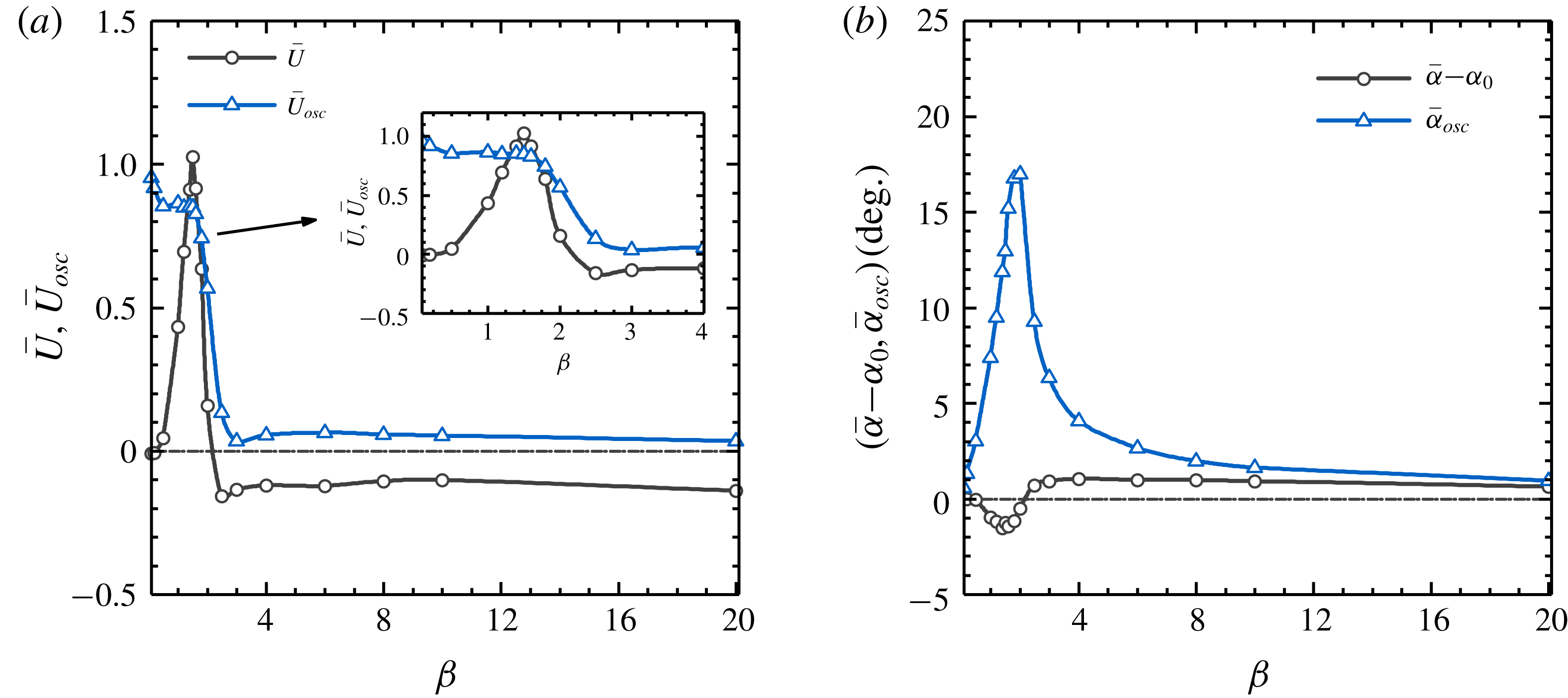
Influences of mass ratio on the performance metrics: (a) averaged vertical speed and amplitude of vertical oscillation; and (b) averaged pitching angle and amplitude of angular oscillation. The inset in (a) is a zoom-in view. The fixed control parameters are:
 $\unicode[STIX]{x1D6FC}_{0}=45^{\circ }$
,
 $\unicode[STIX]{x1D6FE}=17.0$
,
 $\bar{A}=1.0$
,
 $Re=200$
and
 $Fr=8.165$
.

The influence of density on the flyer’s behaviour is studied next. The mass ratio
 $\unicode[STIX]{x1D6FD}$
is allowed to vary in the range of
 $0.1{-}20$
(due to the variation of
 $\unicode[STIX]{x1D70C}_{s}$
), while the dimensionless stiffness and resting angle are kept fixed (
 $\unicode[STIX]{x1D6FE}=17$
,
 $\unicode[STIX]{x1D6FC}_{0}=45^{\circ }$
). The variations of the performance metrics with increasing
 $\unicode[STIX]{x1D6FD}$
are shown in figure 3. From figure 3(a), it is seen that the flyer can sustain hovering approximately at very low mass ratio. A ‘pulse’ in the averaged vertical speed is observed near
 $\unicode[STIX]{x1D6FD}=2.0$
(where the peak speed of
 $1.05$
is reached). The averaged vertical speed then decreases rapidly with increasing
 $\unicode[STIX]{x1D6FD}$
, and reaches the largest descending speed of
 $-0.2$
at
 $\unicode[STIX]{x1D6FD}=2.5$
. In the range of
 $2.5<\unicode[STIX]{x1D6FD}<10.0$
, the averaged vertical speed first rises slightly and then levels off with increasing
 $\unicode[STIX]{x1D6FD}$
. The averaged vertical speed slightly declines if
 $\unicode[STIX]{x1D6FD}$
is further increased. The amplitudes of vertical oscillation appear to be quite high at low mass ratio (the amplitude reaches
 $1.0$
at
 $\unicode[STIX]{x1D6FD}=0.1$
). This is because the flyer tends to follow the oscillatory background flow when its inertia is small. A steep ‘cliff’ in the amplitude of vertical oscillation is observed near
 $\unicode[STIX]{x1D6FD}=2.0$
(where the peak averaged vertical speed is reached). In the range of
 $2.0<\unicode[STIX]{x1D6FD}<3.0$
, the amplitude of vertical oscillation rapidly declines and reaches the (local) minimum value of 0.05 at
 $\unicode[STIX]{x1D6FD}=3.0$
. The amplitude of vertical oscillation then slightly rises and levels off with increasing mass ratio.
In the entire range of mass ratio considered, the averaged opening angle is always very close to the resting angle (see figure 3
b). The largest deviation never exceeds
 $\pm 2^{\circ }$
. The amplitude of angular oscillation is quite small at very low mass ratio. A ‘pulse’ in the amplitude of angular oscillation is also observed near
 $\unicode[STIX]{x1D6FD}=2.0$
, where a peak amplitude of
 $17^{\circ }$
is reached). The amplitude of angular oscillation then declines very rapidly with increasing mass ratio and becomes extremely low at high mass ratio (
 $\unicode[STIX]{x1D6FD}>10.0$
).
The peaked shape in the curve of angular oscillation amplitude at a certain mass ratio also hints at the occurrence of resonance. In this case, the natural frequency of the system is tuned by the variation of mass ratio. The low-amplitude angular oscillations at low and high mass ratios can be explained by the remoteness from the resonant region. The concurrent appearance of the peaks in the averaged vertical speed and the amplitude of angular oscillation again suggests the possible association between the weight-supporting capability and the occurrence of resonance.
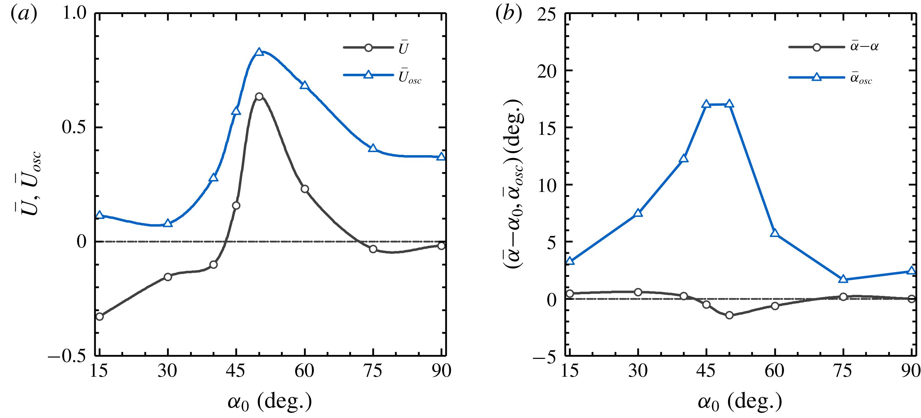
Influences of resting angle on the performance metrics: (a) averaged vertical speed and amplitude of vertical oscillation; and (b) averaged pitching angle and amplitude of angular oscillation. The fixed control parameters are:
 $\unicode[STIX]{x1D6FD}=2.0$
,
 $\unicode[STIX]{x1D6FE}=17.0$
,
 $\bar{A}=1.0$
,
 $Re=200$
and
 $Fr=8.165$
.

Similarly, the influence of resting angle is studied by allowing
 $\unicode[STIX]{x1D6FC}_{0}$
to vary in the range of
 $15^{\circ }{-}90^{\circ }$
, while keeping the other two dimensionless quantities fixed (
 $\unicode[STIX]{x1D6FD}=2.0$
,
 $\unicode[STIX]{x1D6FE}=17.0$
). The variations of the performance metrics with increasing
 $\unicode[STIX]{x1D6FC}_{0}$
are shown in figure 4. It is seen that, at very small resting angles, the flyers descend at relatively high speed. Moreover, we also found that, at small resting angles, the postural stability of the flyers with concave-down configuration cannot be preserved. (The postural stability behaviours will be further discussed in § 4.6.) The flyer can achieve the approximate hovering state at resting angles of
 $45^{\circ }$
and
 $70^{\circ }$
. At the resting angle of
 $90^{\circ }$
(corresponding to the shape of a flat plate), the flyer descends gently. It seems that
 $50^{\circ }$
is the optimal resting angle in terms of the weight-supporting capability. At this resting angle, a peak averaged vertical speed of
 $0.62$
is reached. It appears that the averaged opening angle never deviates too much from the resting angle (the differences are within
 $\pm 2^{\circ }$
) with the variation of
 $\unicode[STIX]{x1D6FC}_{0}$
. It is also found that the amplitudes of the vertical and the angular oscillations reach the maximum values at nearly the same resting angle of
 $50^{\circ }$
. The peaked shape in the curve of angular oscillation amplitude near a certain resting angle again hints at the occurrence of resonance. In this case, the matching of the natural frequency with the driving frequency is achieved by tuning the resting angle (the dependence of the natural frequency on resting angle is discussed in appendix C).
4.3 Actuation efforts required for hovering
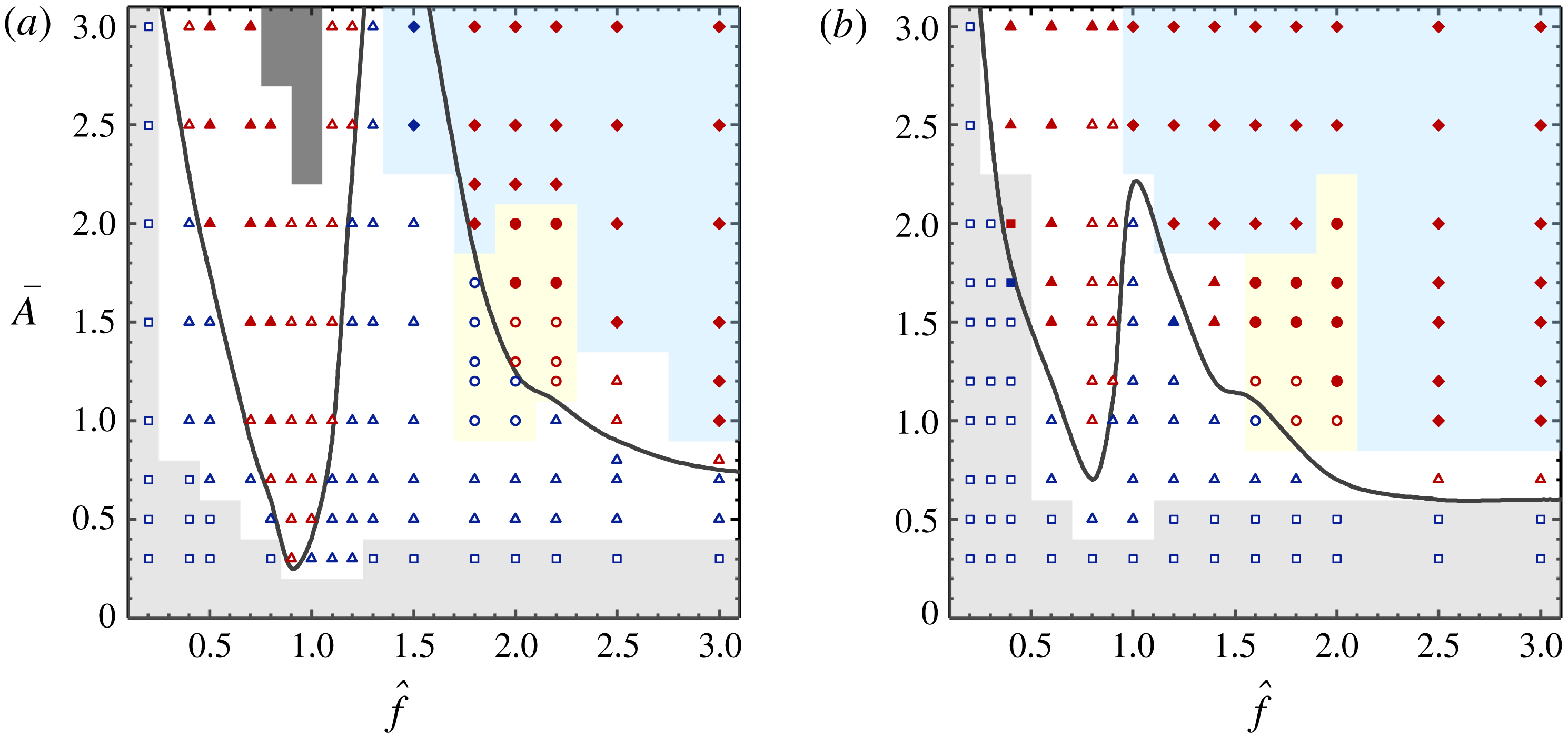
The map of locomotion states, angular oscillation patterns and wake symmetry properties in the two-dimensional space of (
 $\hat{f},\bar{A}$
), for a given flexible flyer (
 $\unicode[STIX]{x1D6FC}_{0}=45^{\circ },~\unicode[STIX]{x1D6FD}=2.0$
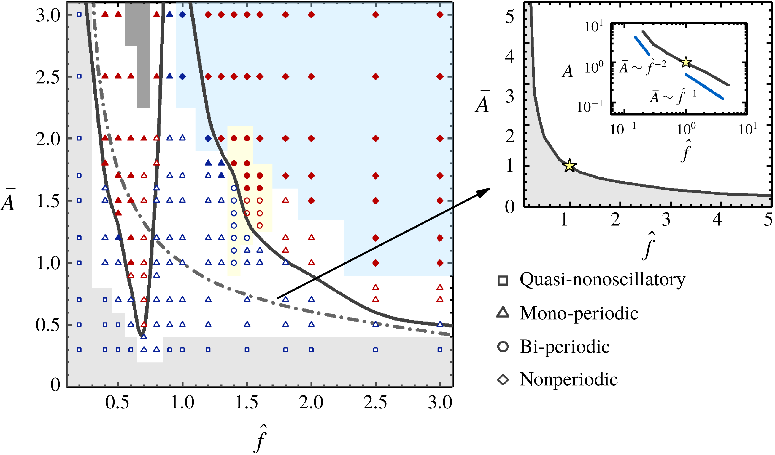
). Squares, triangles, circles and rhombuses denote the quasi-non-oscillatory, mono-periodic, bi-periodic and non-periodic angular oscillations, respectively. The symbols with red and blue colours represent the ascending and descending states, respectively. The open and full symbols represent the symmetric and asymmetric wakes, respectively. The black solid line and the grey dash-dotted line denote the hovering curves which separate the ascending and descending regions, for the flexible and the rigid flyer, respectively. The region painted with dark grey colour represents the driving conditions under which the two foils of the flexible flyer collide with each other. The smaller plot at the top right displays the hovering curve for the rigid flyer in the extended ranges of frequency and amplitude. The star on the hovering curve denotes the reference case with
 $\hat{f}=1.0$
and
 $\bar{A}=1.0$
.

In this section, we enquire into the actuation efforts needed to sustain hovering. To this end, we conduct simulations by varying the driving conditions (i.e. frequency and amplitude) from case to case, while keeping other physical parameters fixed. We first select a base frequency
 $f^{\ast }$
, and the dimensionless quantities based on
 $f^{\ast }$
are prescribed as
 $\unicode[STIX]{x1D6FE}^{\ast }=10,~Re^{\ast }=200$
and
 $Fr^{\ast }=8.165$
. Other dimensionless variables that are fixed in the simulations are
 $\unicode[STIX]{x1D6FC}_{0}=45^{\circ }$
and
 $\unicode[STIX]{x1D6FD}=2.0$
. The frequency ratio
 $\hat{f}=f/f^{\ast }$
is then allowed to vary in the range of
 $0.1{-}3.0$
and the dimensionless quantities may vary accordingly. To be more specific,
 $\unicode[STIX]{x1D6FE}=\unicode[STIX]{x1D6FE}^{\ast }\hat{f}^{-2}$
,
 $Fr=Fr^{\ast }\hat{f}$
and
 $Re=Re^{\ast }\hat{f}$
. At the same time, the dimensionless amplitude
 $\bar{A}$
is allowed to vary in the range of
 $0.3{-}3.0$
. To contrast the actuation efforts needed for hovering in flexible and rigid flyers, simulations are also conducted on a rigid flyer (by setting an extremely large value of
 $10^{4}$
to
 $\unicode[STIX]{x1D6FE}$
, while keeping other dimensionless variables the same as those for the flexible flyer).
In figure 5, the locomotion states are mapped onto the two-dimensional space of
 $(\,\hat{f},\bar{A})$
and the ascending and descending states are marked with red and blue colours, respectively. Clearly, the demarcation line that separates the region for the ascending state from that for the descending state represents the actuation efforts required to sustain hovering. Such a demarcation line is termed the ‘hovering curve’ hereafter. For the convenience of comparison, the hovering curve for the rigid flyer is also plotted.
From figure 5, it is seen that the shape of the hovering curve for the rigid flyer is hyperbola-like. In the studies of Weathers et al. (Reference Weathers, Folie, Liu, Childress and Zhang2010) and Huang et al. (Reference Huang, Nitsche and Kanso2016), it was found that
 $\bar{A}$
scaled as
 $\hat{f}^{-2}$
and
 $\hat{f}^{-1}$
, at the low- and high-frequency limits, respectively. This implied that, for the rigid flyer to sustain hovering, the required flow acceleration is a constant at low frequency, while the required flow speed is a constant at high frequency. In this work, such power laws with very similar power exponents are also found in the two frequency limits.
The hovering curve for the flexible flyer is of wavy shape. For the flexible flyer to sustain hovering, the trough on this curve at
 $(0.7,0.4)$
represents the minimal actuation efforts required. The hovering curves for the flexible and the rigid flyers intersect at
 $(0.8,1.2)$
, where the efforts required by both flyers are equal. The adding of torsional flexibility may lower (or raise) the efforts needed for hovering when the frequency ratio is below (or above) a critical value of 0.8. Interestingly, the supportive (Childress et al.
Reference Childress, Vandenberghe and Zhang2006) and obstructive (Weathers et al.
Reference Weathers, Folie, Liu, Childress and Zhang2010) effects of flexibility on the passive hovering of a flyer have already been observed experimentally. We conjecture that the two opposing effects of flexibility on hovering efforts were observed in the parameter ranges corresponding to the ‘trough’ and ‘ridge’ on the hovering curve, respectively. However, since no sufficiently detailed information regarding the ranges of driving frequency and bending rigidity in these experiments were available, this conjecture is still contestable. From figure 5, it is also seen that the hovering curves for the flexible and the rigid flyers behave similarly at the low- and high-frequency limits. This can be explained by the fact that the amplitude of angular oscillation in the flexible flyer becomes very low when the driving frequency is kept far away from the resonant frequency.
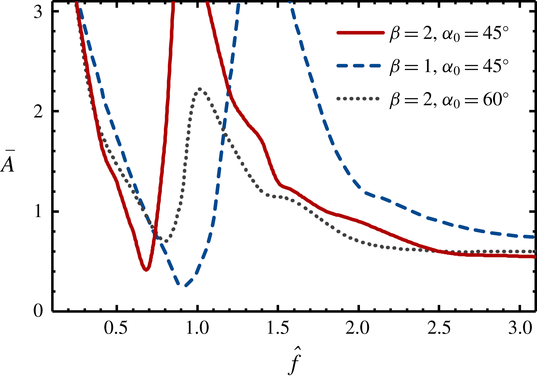
The maps for the locomotion state, the pattern of angular oscillation and the wake symmetry property in the two-dimensional space of
 $(\,\hat{f},\bar{A})$
, for two other given flexible flyers: (a)
 $\unicode[STIX]{x1D6FD}=1.0$
,
 $\unicode[STIX]{x1D6FC}_{0}=45^{\circ }$
, and (b)
 $\unicode[STIX]{x1D6FD}=2.0$
,
 $\unicode[STIX]{x1D6FC}_{0}=60^{\circ }$
. The symbols, colours and lines used here are the same as those for figure 5.

Some additional simulations are also performed to study the influences of mass ratio and resting angle on the hovering curve of the flexible flyer. The maps of locomotion states for two other given flexible flyers (with a different mass ratio or a different resting angle) are shown in figure 6. It is seen that similarities are shared by all three maps, in terms of the wavy shape of the hovering curves, the distribution of the regions with different angular oscillation pattern or different wake symmetry property. The three hovering curves in the three maps shown in figures 5 and 6 are further compared in figure 7. It is seen that the increase of resting angle tends to smooth out the trough and ridge on the hovering curve. Moreover, the variation in mass ratio or resting angle tends to shift the frequency ratio corresponding to the trough on the hovering curve. This shift can be explained by the modulation of natural frequency due to the variation of mass ratio or resting angle (since the trough on the hovering curve is associated with the occurrence of resonance). The relation between hovering efforts and resonance will be explained more precisely below.

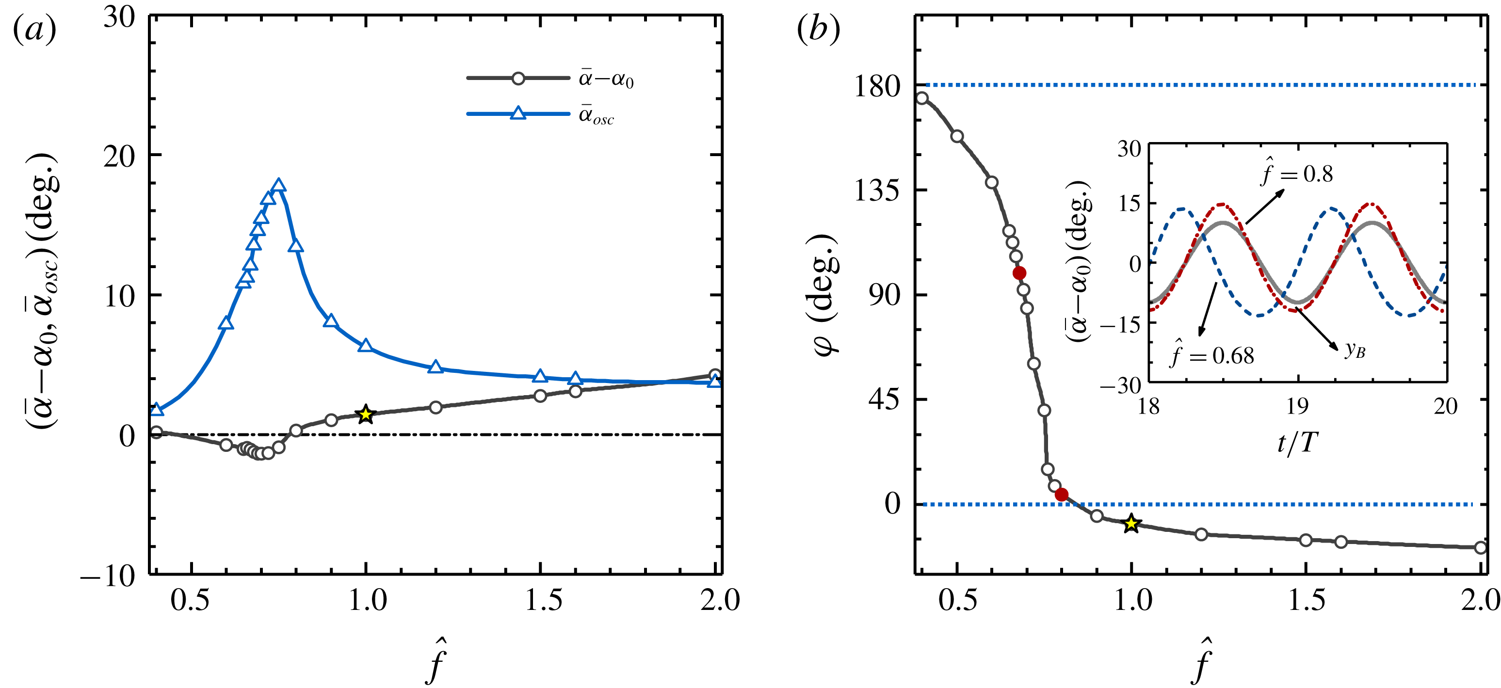
Here an in-depth investigation is conducted to unveil the underlying mechanism that governs the influence of flexibility on the weight-supporting capability. We argue that the influence of flexibility pivots on the modulation of the relative velocity between the flyer and the imposed oscillatory flow due to the involvement of passive angular oscillation. The phase difference between the passive angular oscillation and the background flow and the amplitude of angular oscillation are the two key factors that determine the sign and magnitude of the velocity modulation. An angular oscillation that is anti-phase with respect to the background flow tends to strengthen the effective actuation, while an in-phase angular oscillation tends to attenuate the effective actuation. The amplitude of angular oscillation acts as a proportionality factor which magnifies (or reduces) the effect of phase difference.
Variations of some important quantities associated with the passive angular oscillation with increasing frequency ratio: (a) averaged opening angle and amplitude of angular oscillation, and (b) phase difference between the angular oscillation and the imposed oscillatory flow. The inset of (b) shows the time histories of the opening angle at the frequency ratios of 0.68 and 0.8. The time history of the vertical position of a fluid particle of the imposed background flow is also shown for reference (the oscillation amplitude is adjusted ad hoc for better visual effect). The dimensionless amplitude
 $\bar{A}$
is fixed to 1.0. Other control parameters for the given flexible flyer are the same as those for figure 5. The stars in (a) and (b) denote the averaged opening angle and the phase difference at
 $\hat{f}=1.0$
. The solid circles in (b) denote the phase differences at
 $\hat{f}=0.68$
and
 $\hat{f}=0.8$
.

We focus on the flexible flyer illustrated in figure 5, and examine the variations of amplitude and phase of the angular oscillation with increasing frequency ratio, for a fixed dimensionless amplitude of
 $\bar{A}=1.0$
(see figure 8). First of all, the averaged opening angle is barely affected by flexibility (the largest deviation from the resting angle never exceeds
 $4^{\circ }$
). Thus, the modification of the averaged opening angle is not likely to be the dominant mechanism by which flexibility affects the weight-supporting capability. At low frequencies, the amplitude of angular oscillation is very small and the influence of flexibility on the weight-supporting capability is also insignificant. With the progressive increase of frequency, a narrow peak in the amplitude of angular oscillation appears when the resonant frequency is approached. Meanwhile, the phase difference between the passive angular oscillation and the imposed flow also experiences a sharp change (from
 $180^{\circ }$
to
 $0^{\circ }$
), when the resonant frequency is crossed. Such a transition (from in-phase state to anti-phase state) in the phase difference between the oscillation and the driving is one intrinsic feature of a driven damped oscillatory system (Fitzpatrick Reference Fitzpatrick2013).
Some efforts are also spent here to further quantify the association of the modulation of relative velocity and the increase (or reduction) in the weight-supporting capability. We first introduce the relative vertical velocity between the flyer and the prescribed oscillatory flow (by taking the passive angular oscillation into account), i.e.
 $U_{R}(t)=\dot{\unicode[STIX]{x1D6FC}}(t)\sin [\unicode[STIX]{x1D6FC}(t)]-\bar{A}\sin (2\unicode[STIX]{x03C0}t)$
. The modulation of relative motion is measured by the difference in the root-mean-square (r.m.s.) values of
 $U_{R}$
, for the flexible and the rigid flyers, i.e.
 $\unicode[STIX]{x0394}U_{R}^{rms}=\sqrt{(1/nT)\int _{T_{0}}^{T_{0}+nT}U_{R}^{2}\,\text{d}t}-(\sqrt{2}/2)\bar{A}$
. The averaged vertical velocity
 $\bar{U}$
and the relative velocity
 $U_{R}$
are dimensionless velocities scaled by
 $fL$
. To facilitate a fair comparison among velocities at different driving frequencies, the velocities are rescaled by using
 $f^{\ast }L$
. The relation between the rescaled and the original variables can be expressed as
 $\hat{\unicode[STIX]{x1D719}}=\unicode[STIX]{x1D719}(\,fL/f^{\ast }L)=\unicode[STIX]{x1D719}\hat{f}$
, where
 $\unicode[STIX]{x1D719}$
and
 $\hat{\unicode[STIX]{x1D719}}$
denote the (dimensionless) velocities before and after the rescaling.
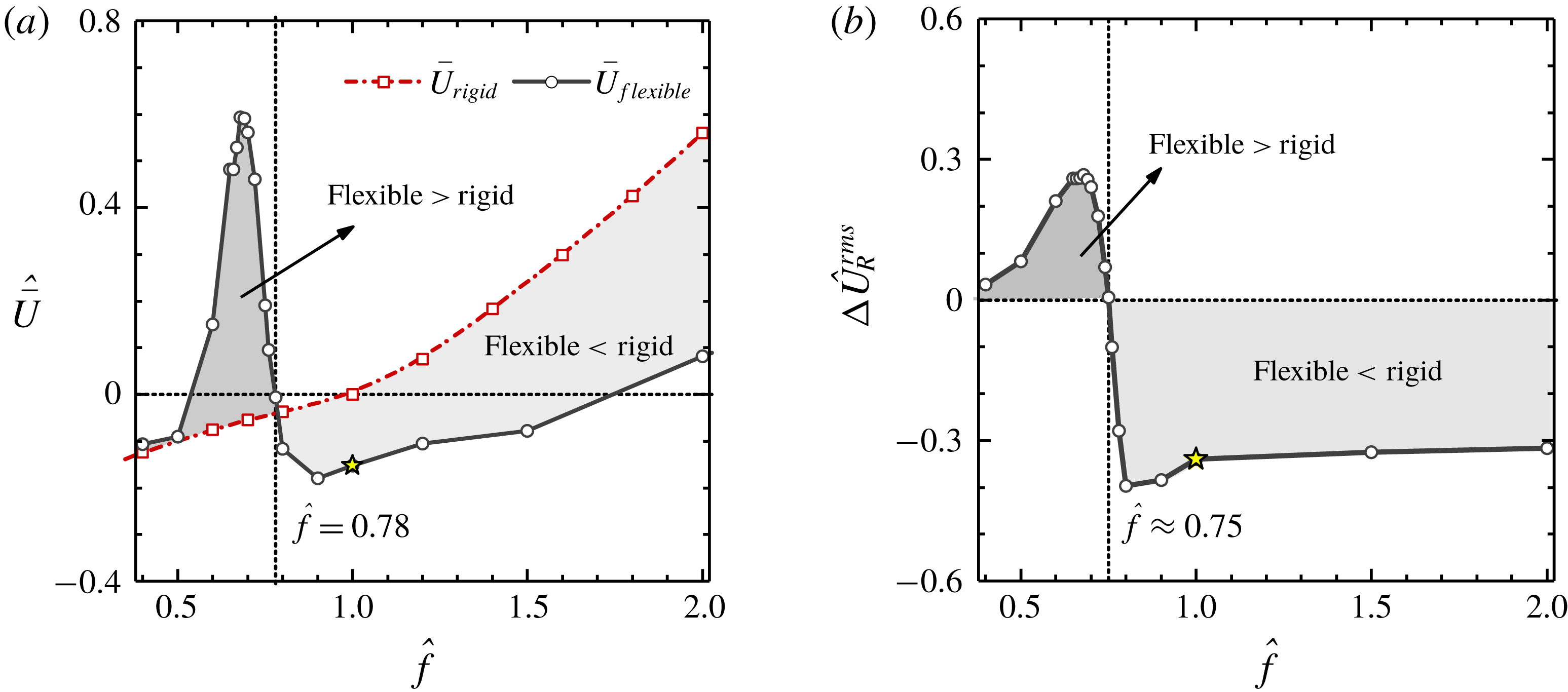
Figure 9(a) shows the variation of the (rescaled) averaged vertical speed (which is a good indicator of the weight-supporting capability) with increasing frequency ratio, for both the flexible and the rigid flyers. It is seen that the vertical speed of the rigid flyer increases monotonically with increasing frequency ratio. At
 $\hat{f}=0.4$
(where the driving frequency is much lower than the resonant frequency), the averaged vertical speeds of both flyers are almost the same. In the vicinity of the resonant frequency, the averaged vertical speed of the flexible flyer rises sharply and becomes much higher than that of the rigid one. Away from the resonant frequency, the averaged vertical speed of the flexible flyer declines rapidly. The speeds of the two flyers become equalized again at
 $\hat{f}=0.78$
. When the driving frequency is further increased, the averaged vertical speed of the flexible flyer stays below that of the rigid flyer.
The association of the difference in averaged vertical speeds for flexible and rigid flyers and the relative vertical velocity between the flyer and the imposed background flow. (a) Averaged vertical speed in the flexible and rigid flyers as a function of frequency ratio; (b) difference in the r.m.s. value of relative vertical velocity as a function of frequency ratio. The dimensionless amplitude
 $\bar{A}$
is fixed to 1.0. Other control parameters for the given flyers are the same as those for figure 5. The stars denote the quantities for the flexible flyer at
 $\hat{f}=1.0$
.

In figure 9(b), the difference in the r.m.s. values of
 $U_{R}$
for the two flyers (after rescaling) is plotted as a function of the frequency ratio. By relating figure 9(b) with figure 9(a), a strong correlation between the difference in the weight-supporting capabilities of the two flyers and the modulation of the relative velocity due to the involvement of passive angular oscillation can be clearly seen. Near the resonant region, the non-monotonic dependence on frequency ratio is exhibited in both figure 9(a) and 9(b). After the resonant region (
 $\hat{f}>1.0$
),
 $\hat{\bar{U}}$
increases monotonically with increasing
 $\hat{f}$
, while
 $\unicode[STIX]{x0394}\hat{U} _{R}^{rms}$
reaches a negative constant value. The similar trend of variation in
 $\hat{\bar{U}}$
with increasing
 $\hat{f}$
, for the flexible and rigid flyers, can be explained by the greatly attenuated passive angular oscillation in the flexible flyer. The lower value of
 $\hat{\bar{U}}$
in the flexible flyer (in comparison with that in the rigid one) can be attributed to (a) an (almost) in-phase passive angular oscillation and (b) a larger averaged opening angle.
4.4 Angular oscillation patterns
For the driving conditions illustrated in figures 5 and 6, the passive angular oscillations of the flexible flyers can be classified into four categories: quasi-non-oscillatory (squares), mono-periodic (triangles), bi-periodic (circles) and non-periodic (rhombuses). From these figures, it is also seen that the regions occupied by the bi-periodic oscillation are rather small, in comparison with the regions occupied by the other patterns.
The time histories of the opening angle, the phase diagrams (spanned by the opening angle and angular velocity) and the power spectra, for the angular oscillations at the frequency ratios of (a)
 $\hat{f}=0.75$
, (b)
 $\hat{f}=1.4$
and (c)
 $\hat{f}=3.0$
. The dimensionless amplitude
 $\bar{A}$
is fixed to 1.0. Other control parameters for the flexible flyer are the same as those for figure 5.

The amplitudes of the angular oscillations in the quasi-non-oscillatory cases are negligibly small (
 $\bar{\unicode[STIX]{x1D6FC}}_{osc}\leqslant 2^{\circ }$
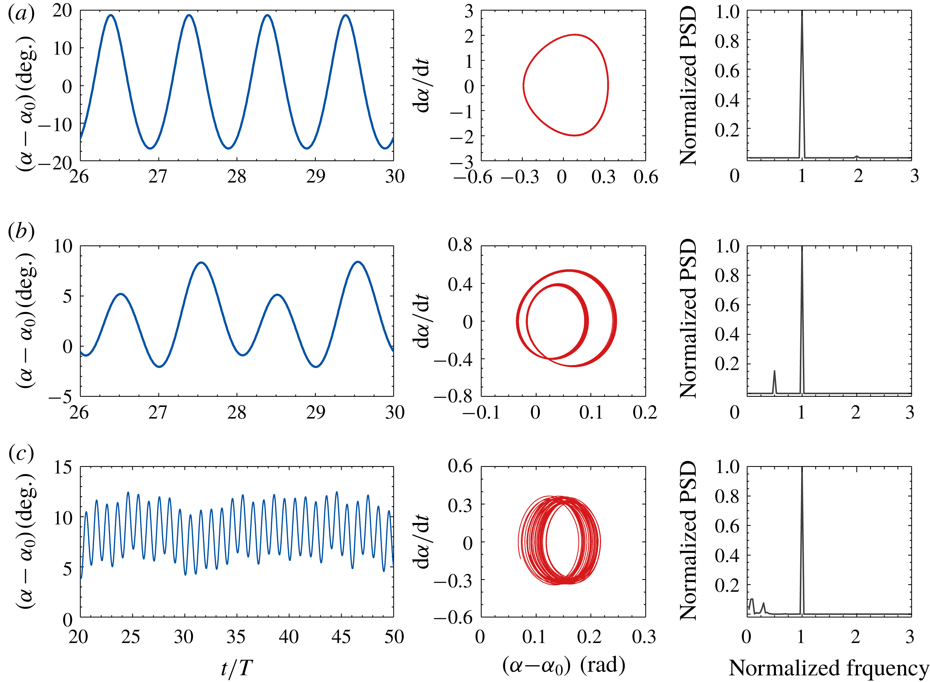
) and the flyer almost behaves as a rigid one. To further illustrate the differences among other patterns of angular oscillations, the time histories of the opening angle, the phase diagram spanned by the opening angle and angular velocity, and the power spectra, for some selected cases, are shown in figure 10. For the mono-periodic case shown in figure 10(a), the passive angular oscillation is slaved to the oscillatory driving motion. (Note that a tiny peak appears in the power spectrum at a frequency that is twice as high as the driving frequency. Since the amplitude of this peak is rather small, the passive angular oscillation is practically mono-periodic.) For the bi-periodic case shown in figure 10(b), two dominant frequencies (i.e. the driving frequency and half of the driving frequency) are observed. For the non-periodic case shown in figure 10(c), the dominant frequency is still the driving frequency, but some small peaks are also observed at lower frequencies. In a previous study on a pinned and rotatable flexible flyer placed in an oscillating flow (Huang et al.
Reference Huang, Ristroph, Luhar and Kanso2018), the passive angular oscillations were found to be mono-periodic and always slaved to the imposed oscillatory flow, irrespective of the driving conditions. We still lack an explanation on the difference in the angular oscillation patterns found in these two studies.
4.5 Wake symmetry properties
Although the left–right symmetry with respect to the centreline of the flyer is ensured in the initial and boundary conditions (see § 3.2), wake symmetry breaking may occur spontaneously under certain circumstances. Since no physical perturbations are imposed, the wake symmetry breaking is triggered solely by the numerical perturbations. The capability (or incapability) of preserving wake symmetry may have a large impact on the postural stability of the flyer, since wake asymmetry is unavoidably accompanied by lateral and rotational motions (the postural stability behaviours will be addressed in § 4.6).
The wake symmetry properties for the flexible flyer under various driving conditions are assessed after a long-time evolution of the flow field (
 $T>40$
). In figures 5 and 6, the symmetric and asymmetric wakes are marked with hollow and solid symbols, respectively. From these figures, some connections between the wake symmetry property and the locomotion state can be recognized. For the descending cases, wake symmetry can be preserved under most situations. The only exceptions exist in the situation of very high oscillating amplitude or very small descending speed (i.e. in the vicinity of the hovering curve). On the contrary, the wakes of an ascending flyer are generally more susceptible to symmetry-breaking instability. For an ascending flyer, wake symmetry can only be preserved near ‘narrow bands’ adjacent to the hovering curve.
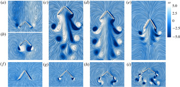
The wake patterns of the flexible flyer for nine selected cases, with a dimensionless amplitude of 1.0 and the frequency ratios of (a)
 $\hat{f}=0.2$
, (b)
 $\hat{f}=0.5$
, (c)
 $\hat{f}=0.68$
, (d)
 $\hat{f}=0.7$
, (e)
 $\hat{f}=0.75$
, (f)
 $\hat{f}=0.78$
, (g)
 $\hat{f}=1.4$
, (h)
 $\hat{f}=2.0$
and (i)
 $\hat{f}=3.0$
. The values of other control parameters are the same as those for figure 5. The streamlines and the contours of dimensionless vorticity
 $\unicode[STIX]{x1D714}$
(vorticity scaled by
 $f$
) are used to visualize the vortex structures.

Some representative wake patterns of the flexible flyer corresponding to nine cases selected from figure 5 are shown in figure 11. The frequency ratio is in the range of
 $0.2{-}3.0$
and the dimensionless amplitude is fixed to
 $1.0$
. At
 $\hat{f}=0.2$
, the flyer descends steadily and the wake is clear of any large vortex structures such as the Kármán vortex street (see figure 11
a). This can be explained by the fact that the descending speed is still not high enough. At
 $\hat{f}=0.5$
, the approximate hovering state is achieved (actually the flyer still descends very gently). It is seen that two vortex dipoles are stably attached to the two free ends (see figure 11
b). The downward jets induced by the dipoles are indicative of the production of weight-supporting forces. Moreover, no other large vortex structures are visible in the far wake. Clearly, wake symmetry is preserved in the two cases above. At
 $\hat{f}=0.68$
and
 $\hat{f}=0.7$
(where the driving frequencies are close to the resonant frequency), since the hovering curve is crossed (cf. figure 5), large ascending speeds are now achieved. The presence of two queues of vortex dipoles below the ascending flyer is the prominent feature of the wake patterns (see figure 11
c,d). These vortex structures resemble those produced by the active jellyfish-like flyer (Fang et al.
Reference Fang, Ho, Ristroph and Shelley2017; Zhang et al.
Reference Zhang, He, Wang and Zhang2018). As can be seen here, wake symmetry is preserved in the case of
 $\hat{f}=0.7$
, but not in the case of
 $\hat{f}=0.68$
. According to the analysis in Zhang et al. (Reference Zhang, He, Wang and Zhang2018), the horizontal component of the dipole-induced velocity is the key factor that determines the wake symmetry property. A large dipole-induced horizontal velocity that points outwards from the centreline tends to separate the two queues of dipoles apart and mitigate the interactions between them. This favours the preservation of wake symmetry. At
 $\hat{f}=0.75$
, the wake symmetry is also preserved. The weakened strength of the dipoles signifies a much reduced ascending speed (see figure 11
e). At
 $\hat{f}=0.78$
, the frequency is now removed away from the resonant region and the hovering curve is crossed again. Similar to the case of
 $\hat{f}=0.2$
, the wake pattern also signifies a falling motion (see figure 11
f). The difference in the wake patterns of these two cases reflects the difference in the falling speed. At
 $\hat{f}=1.4$
, the descending speed is reduced to some extent and two dipoles emerge at the two free ends (see figure 11
g). At
 $\hat{f}=2.0$
, the hovering curve is crossed once more and a small ascending speed is achieved. The shedding of vortex dipoles near the free ends can be seen and wake symmetry is preserved. Unlike the case of
 $\hat{f}=0.7$
, at this frequency the vortex structures dissipate very rapidly with increased distance from the flyer and the two complete queues of dipoles are not observed (see figure 11
h). At
 $\hat{f}=3.0$
, the ascending velocity becomes much larger with increased actuation efforts. The two queues of dipoles behind the trailing ends reappear, together with an asymmetric wake (see figure 11
i). Comparing with the case at
 $\hat{f}=0.68$
, the two queues of dipoles now separate further apart from each other. Thus, the asymmetric wake is not likely to be initiated by the strong interaction between two queues of dipoles. Instead, we believe that symmetry breaking is triggered by the inherent wake instability at a relatively high (flapping) Reynolds number. In a previous study on the swimming of a two-dimensional jellyfish model, asymmetric wakes were also found to arise spontaneously at high Reynolds numbers (Alben, Miller & Peng Reference Alben, Miller and Peng2013).
The wake patterns of the rigid flyer for four selected cases, with the dimensionless amplitude of 1.0 and the frequency ratios of: (a)
 $\hat{f}=0.2$
, (b)
 $\hat{f}=0.7$
, (c)
 $\hat{f}=2.0$
and (d)
 $\hat{f}=3.0$
. The values of other control parameters are the same as those for figure 5. The streamlines and the contours of dimensionless vorticity
 $\unicode[STIX]{x1D714}$
(vorticity scaled by
 $f$
) are used to visualize the vortex structures.

To reveal the influence of flexibility on the wake symmetry property, the wake patterns of a rigid flyer under similar driving conditions are shown in figure 12 for comparison. At
 $\hat{f}=0.2$
, the rigid flyer descends steadily and the wake pattern is similar to that of the flexible flyer at the same frequency (see figure 12
a). This is because the passive angular oscillation of the flexible flyer is insignificant at this frequency, due to the remoteness of the driving frequency from the natural frequency. Thus, the flexible flyer behaves practically like a rigid one. At
 $\hat{f}=0.7$
, the driving frequency is moved closer towards the hovering curve (but the hovering curve is still not crossed) and the flyer descends very gently (see figure 12
b). The wake pattern resembles the one produced by the flexible flyer at
 $\hat{f}=0.5$
(cf. figure 11
b). At
 $\hat{f}=2.0$
, the hovering curve is crossed and an ascending speed is achieved. The two queues of dipoles are now visible, together with an asymmetric wake (see figure 12
c). In this case, symmetry breaking is likely to be triggered by the strong interaction between the two queues of dipoles. To some extent, the wake structure at this frequency resembles that of the flexible flyer at
 $\hat{f}=0.68$
(cf. figure 11
c), although the dipoles are more tightly squeezed towards the centreline. At
 $\hat{f}=3.0$
, the ascending speed of the rigid flyer increases further and the two queues of dipoles separate apart from each other (see figure 12
d). The asymmetric wake pattern at this frequency resembles that produced by the flexible flyer at the same frequency. Similar to the flexible case at
 $\hat{f}=3.0$
, the wake symmetry breaking is likely to be initiated by the inherent instability at high (flapping) Reynolds numbers. In brief, the wake patterns in flexible and rigid flyers are fundamentally different only when the driving frequencies are close to the resonant frequency.
4.6 Postural stability behaviours
In addition to the weight-supporting capability, the postural stability behaviour of the flyer is also of great importance to hovering. In the study of actuation efforts required for hovering, only the concave-down configuration with an upright initial posture (i.e.
 $\unicode[STIX]{x1D703}(0)=0$
) is considered. It turns out that, under certain driving conditions, the flyer is not capable of maintaining the upright posture and a non-zero inclination angle (together with a lateral motion) may spontaneously emerge afterwards.
In this section, we conduct a systematic investigation into the postural stability behaviours of the given flyers under the same actuation conditions as those illustrated in figure 5. We consider both the concave-down and the concave-up configurations, and impose non-zero perturbations to the initial inclination angle while keeping
 $\dot{\unicode[STIX]{x1D703}}(0)=0$
. To be more specific, for the concave-down configuration and the concave-up configuration, the initial inclination angles are set to
 $\unicode[STIX]{x03C0}/18$
and
 $17\unicode[STIX]{x03C0}/18$
, respectively.
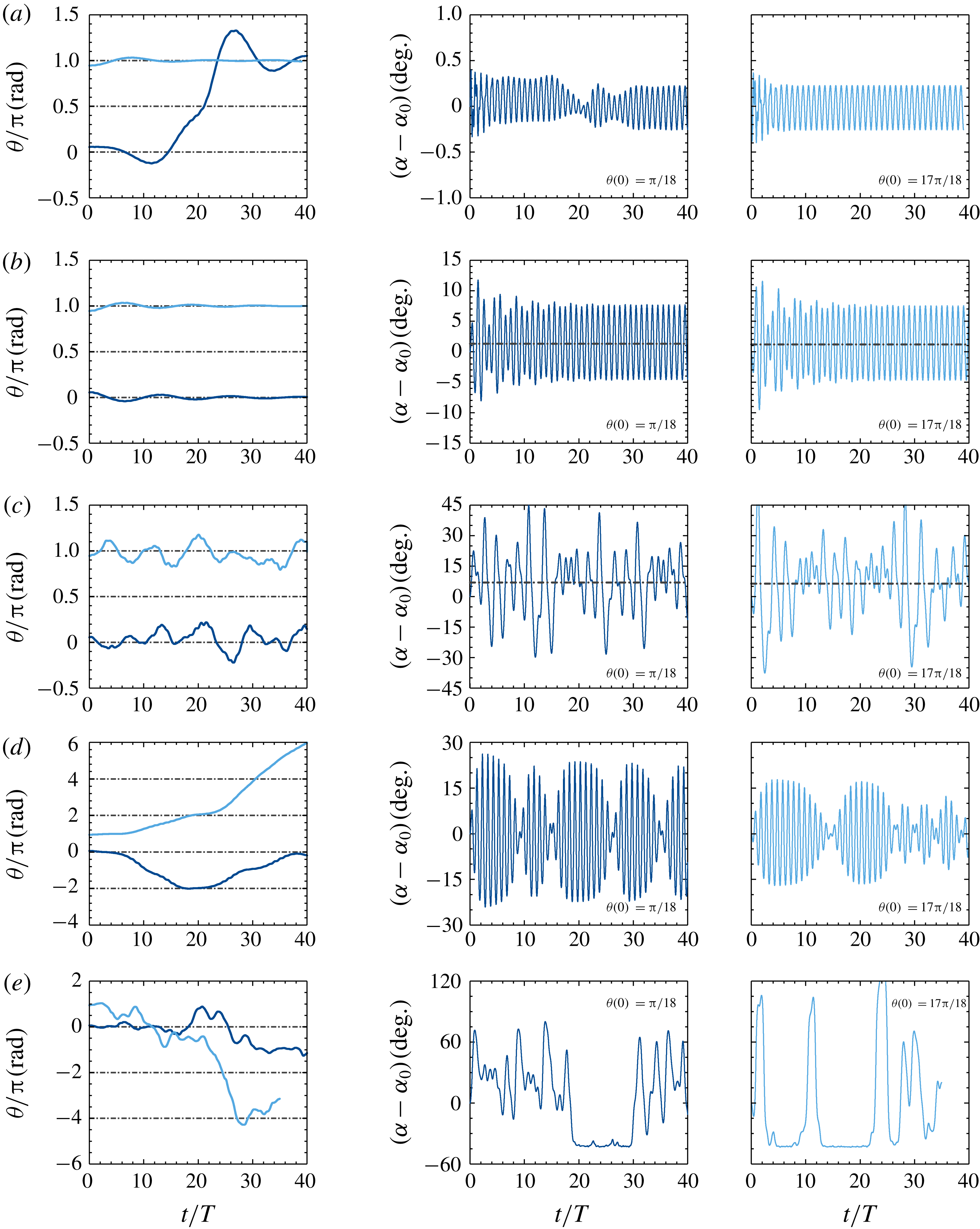
Time histories of the inclination angle and the opening angle for the flexible flyer with different postural stability behaviours: (a) V-stable behaviour (
 $\,\hat{f}=0.2,~\bar{A}=0.5$
); (b) bi-stable behaviour (upright subtype,
 $\hat{f}=1.0,~\bar{A}=1.0$
); (c) bi-stable behaviour (chaotic-like swinging subtype,
 $\hat{f}=2.0,~\bar{A}=2.0$
); (d) unstable behaviour (continuous rotation subtype,
 $\hat{f}=0.7,~\bar{A}=2.0$
); and (e) unstable behaviour (chaotic-like flight subtype,
 $\hat{f}=3.0,~\bar{A}=3.0$
). The other control parameters are the same as those used in figure 5.

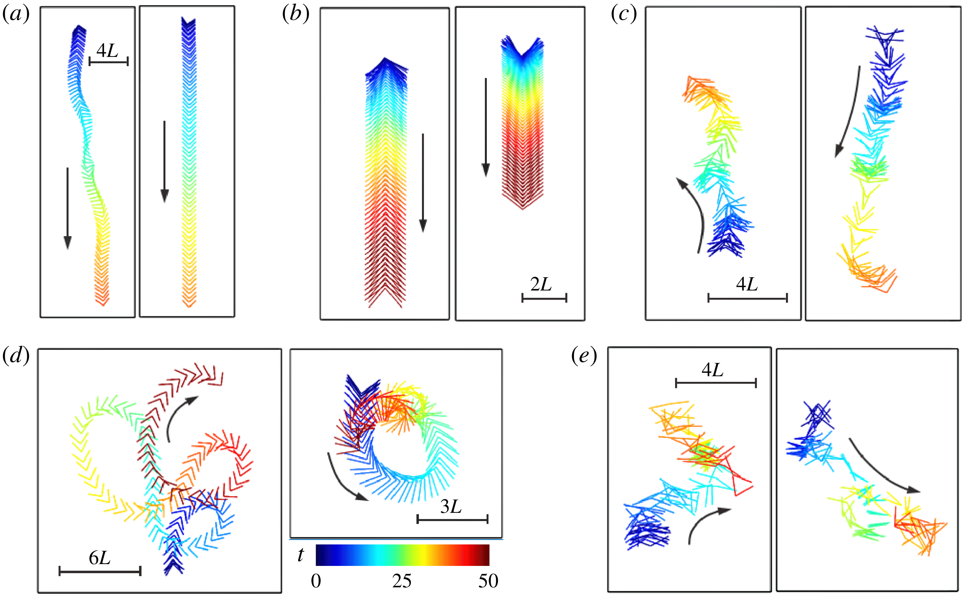
Trajectories of the flexible flyer with different postural stability behaviours: (a) V-stable behaviour; (b) bi-stable behaviour (upright subtype); (c) bi-stable behaviour (chaotic-like swinging subtype); (d) unstable behaviour (continuous rotation subtype); and (e) unstable behaviour (chaotic-like flight subtype). The shape of the flyer is coloured by time (from blue to red). The control parameters used in this figure are the same as those used in figure 13.

The postural stability behaviours of the flyer are then assessed by examining the time histories of inclination angle. Among all the cases studied, three different behaviours pertinent to postural stability are identified: V-stable behaviour in which only the concave-up configuration is the stable equilibrium solution (figure 13
a); bi-stable behaviour in which both the concave-up and the concave-down configurations are the stable equilibrium solutions (figures 13
b,c); and unstable behaviour in which converged inclination angles are not reached (figure 13
d,e). Here we also distinguish between two subtypes of bi-stable behaviours: upright subtype in which
 $\unicode[STIX]{x1D703}$
converges to 0 or
 $\unicode[STIX]{x03C0}$
(figure 13
b), and chaotic-like swinging subtype in which the deviation of the inclination angle from 0 or
 $\unicode[STIX]{x03C0}$
is bounded (figure 13
c). The unstable behaviours can also be further classified into two subtypes: continuous rotation (figure 13
d) and chaotic-like flight (figure 13
e).
In addition to the time histories of the inclination angle, the time histories of the opening angle are also shown in figure 13. It is seen that the passive angular oscillations that accompany the V-stable behaviour and the upright subtype of the bi-stable behaviour are mono-periodic and slaved to the driving (figure 13
a,b). Since the amplitude of angular oscillation associated with the V-stable behaviour is always less than
 $0.5^{\circ }$
, the flyer practically behaves like a rigid falling object. For the chaotic-like swinging subtype of the bi-stable behaviour, the accompanying angular oscillation is chaotic-like in itself (figure 13
c). The angular oscillation that accompanies the continuous rotation subtype of the unstable behaviour is actually the superposition of a low-frequency rotation on a mono-periodic oscillation (which is slaved to the driving) (figure 13
d). For the chaotic-like flight subtype of the unstable behaviour, the accompanying angular oscillation is also chaotic-like in itself (figure 13
e).
The trajectories of the flexible flyer associated with different postural stability behaviours are shown in figure 14. For the V-stable behaviour and the upright subtype of the bi-stable behaviour, the flyer almost falls along a straight line (figure 14 a,b). For the chaotic-like swinging subtype of the bi-stable behaviour, a flyer with the concave-down configuration tends to rise while a flyer with the concave-up configuration tends to fall (figure 14 c). The distinction between the trajectories of the two subtypes of the unstable behaviours can be clearly seen by contrasting figure 14(d) with 14(e).
In figure 15(a), different types of postural stability behaviours of the flexible flyer are denoted by different symbols in the space of
 $(\,\hat{f},\bar{A})$
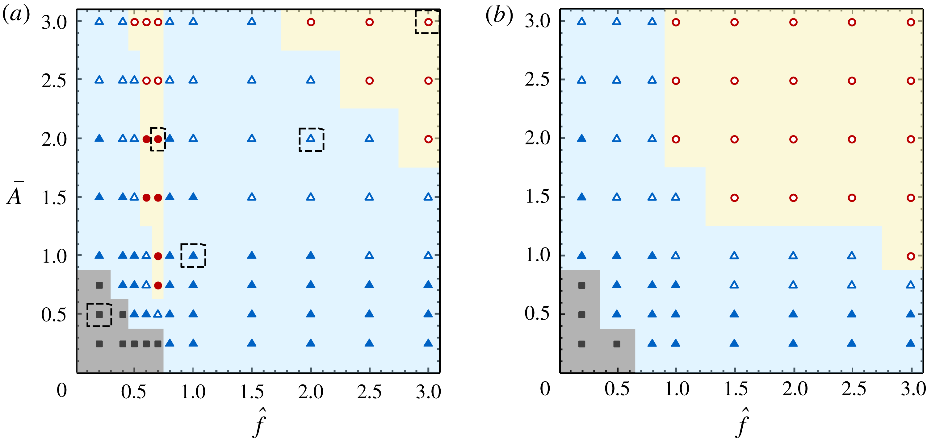
. It is seen that the V-stable behaviour occupies a small region in the lower left corner, which represents very low actuation efforts. The largest region representing moderate actuation efforts is occupied by the bi-stable behaviours (with increasing actuation efforts, the bi-stable behaviours transit from the upright subtype to the chaotic-like swinging subtype). The upper right corner, which represents very high actuation efforts, is occupied by the chaotic-like flight subtype of the unstable behaviour. The unstable behaviours also occupy a narrow wedge-shaped region which splits the region of the bi-stable behaviours into two parts. Within this wedge-shaped region, the unstable behaviours transit from the continuous rotation subtype to the chaotic-like flight subtype when the driving amplitude exceeds a critical value.
The map of postural stability behaviours in the space of
 $(\,\hat{f},\bar{A})$
, for (a) the flexible flyer and (b) the rigid flyer. The values of the specified parameters are the same as those for figure 5. Solid square, V-stable behaviour; solid triangle, bi-stable behaviour (upright subtype); open triangle, bi-stable behaviour (chaotic-like swinging subtype); solid circle, unstable behaviour (continuous rotation subtype); open circle, unstable behaviour (chaotic-like flight subtype). The cases highlighted in the dashed boxes in panel (a) correspond to the five cases shown in figure 14.

The association of the postural stability behaviours and the wake symmetry properties can be established by relating figure 15(a) with figures 5 and 11. (The following discussion is only relevant to the flexible flyer with concave-down configuration.) The upright subtype of the bi-stable behaviour is always accompanied by the recovery of wake symmetry after the perturbations. The unstable behaviours (including the continuous rotation and the chaotic-like flight subtypes) are always accompanied by wake asymmetry. The continuous rotation subtype of the unstable behaviour is a unique locomotion style which only exists in the flexible flyers. This locomotion style can be linked with the distinct wake pattern shown in figure 11(c). The wake is slightly asymmetric and all vortex dipoles are tightly squeezed towards the centreline. This wake pattern signifies a high-speed forward motion produced by strong propulsion and a much weaker sideways motion due to asymmetry. In most cases, the chaotic-like swinging subtype of the bi-stable behaviour is also accompanied by wake asymmetry. However, for this subtype of the bi-stable behaviour, there exist a few cases in which wake symmetry is still preserved (cf. figure 5). The seeming inconsistency in these cases can be rationalized as follows. In assessing the wake symmetry properties in § 4.5, the perturbations are numerical noise and are much smaller in magnitude than those imposed in the study of the postural stability behaviours. Thus, it may take a much longer time before wake asymmetry eventually emerges.
Similarly, figure 15(b) shows the map of postural stability behaviours for the rigid flyer in the space of
 $(\,\hat{f},\bar{A})$
. The influence of flexibility on the postural stability behaviours can be clearly seen by contrasting figure 15(b) with figure 15(a). It is seen that the area and shape of the region occupied by the V-stable behaviour are barely influenced by flexibility. This is because the flexible flyer practically behaves like a rigid one when actuation efforts are very low. Moreover, the demarcation line that separates the two subtypes of the bi-stable behaviours is only slightly modulated by flexibility. The noticeable differences between these two panels are found in the region representing moderate actuation efforts. First, the continuous rotation subtype of the unstable behaviour is not observed in the rigid flyer. Second, the wedge-shaped region in the stability map of the flexible flyer (which is occupied by the unstable behaviours) does not show up in the stability map of the rigid flyer. Instead, in the stability map of the rigid flyer, a gradual transition from the V-stable behaviour to the bi-stable behaviours and then to the unstable behaviours is observed with increasing actuation efforts. Last, in the map of the rigid flyer, the area of the region for the unstable behaviour is much larger, in comparison with the map of the flexible flyer. It is observed that, when the frequency ratio is larger than one, the rigid flyer transits from the bi-stable state to the unstable state at relatively lower amplitude (in comparison with the flexible flyer). This is because the effective actuation in the rigid flyer is much stronger due to the absence of (in-phase) passive angular oscillation. To summarize, adding flexibility can either initiate or suppress postural instability of the flyer, depending on the driving condition.
Here the postural stability behaviours of the unconstrained flyers in the present study are also compared with those of the pinned and rotatable flyers placed in oscillatory flows (Huang et al.
Reference Huang, Ristroph, Luhar and Kanso2018). In Huang et al. (Reference Huang, Ristroph, Luhar and Kanso2018),
 $\unicode[STIX]{x039B}$
-stable, bi-stable and oblique-stable behaviours are found. The bi-stable behaviour contains three subtypes, namely, upright, quasi-periodic swinging and chaotic-like swinging. In the current study, V-stable, bi-stable and unstable behaviours are found. The bi-stable behaviour contains two subtypes, namely, upright and chaotic-like swinging. The unstable behaviour also contains two subtypes, namely, continuous rotation and chaotic-like flight. The different behaviours reported in these two studies stem from the different constraining conditions on the flyer. A more detailed discussion regarding the comparison of stability properties in the two systems is provided as follows.
The
 $\unicode[STIX]{x039B}$
-stable behaviour (or the V-stable behaviour) is observed when the actuation is very weak. Under such circumstances, the effects of flexibility are also insignificant. In Huang et al. (Reference Huang, Ristroph, Luhar and Kanso2018), the pinned flyer behaves just like a pendulum or an inverted pendulum. The force of gravity tends to stabilize a flyer in the
 $\unicode[STIX]{x039B}$
-configuration, while it destabilizes the flyer in the V-configuration. In the present study, the flyer behaves like a free-falling rigid object. Gravity does not affect the stability since the flyer is allowed to move freely. The imbalanced aerodynamic torques on the two links (when the flyer is slightly tilted) can explain the V-stable behaviour of the flyer (see appendix D for the details).
In both studies, the bi-stable behaviours are observed at moderate or strong actuation. In Huang et al. (Reference Huang, Ristroph, Luhar and Kanso2018), the bi-stable behaviour is explained by the existence of two ‘wells’ in the rotational potential at
 $\unicode[STIX]{x1D703}=0$
and
 $\unicode[STIX]{x1D703}=\unicode[STIX]{x03C0}$
, based on an aerodynamic model which accounts for the interaction between the flyer and the oscillating flow. These two ‘wells’ in the rotational potential also shape the bi-stable behaviour in the current study. The absence of the quasi-periodic swinging subtype of the bi-stable behaviour in the current study is due to the sideways motions which prevent the establishment of periodicity.
The unstable behaviour (in which the inclination angle becomes unbounded) is found in the current study but not in Huang et al. (Reference Huang, Ristroph, Luhar and Kanso2018). The oblique-stable behaviour (in which stability can be reached at inclined orientations) is found in Huang et al. (Reference Huang, Ristroph, Luhar and Kanso2018) but not in the current study. The explanations for these phenomena are still lacking. We conjecture that the differences mentioned above are related to the linear displacements, which are only permitted in the current study.
5 Conclusions
We considered the passive flights of a flexible
 $\unicode[STIX]{x039B}$
-flyer in a vertically oscillating airflow with zero mean stream. The flexibility of the flyer was introduced by a torsion spring installed at the hinged joint. The results of this study provided new insight into the mechanism by which flexibility affected the passive flight of a flyer in an oscillatory airflow.
We first studied the influences of several parameters (such as spring stiffness, density and resting angle) on the flight dynamics of the flyer. The study was conducted under a fixed actuation condition and on the concave-down configuration only. It was found that the amplitudes of passive angular oscillations increased markedly at particular parameter values. This hinted that resonance may occur at these parameter values due to the matching of natural frequency with the driving frequency. The concurrent increase in the averaged vertical speed near these parameter values suggested that the weight-supporting capability can be strongly affected by flexibility.
We then focused on the actuation efforts (i.e. driving frequency and amplitude) that are needed in the hovering of the given (flexible and rigid) flyers with concave-down configuration. It was found that the weight-supporting capabilities in flexible and rigid flyers can be significantly different when the driving frequency approached the resonant frequency of the flexible flyer. Whether the weight-supporting capability was enhanced or reduced by adding flexibility primarily depended on whether the relative motion between the flyer and the imposed background flow was strengthened or weakened by the passive angular oscillation.
We also examined the angular oscillation patterns and the wake symmetry properties of the given flyers under various driving conditions. The passive angular oscillations observed in the flexible flyers can be further categorized into four categories, namely, quasi-non-oscillatory, mono-periodic, bi-periodic and non-periodic. The wake patterns in flexible and rigid flyers were found to be very different only when the driving frequency approached the resonant frequency. In the frequency range where flexibility significantly enhanced the weight-supporting capability, wake symmetry can be preserved if the driving frequencies were kept slightly higher than the resonant frequency.
Finally, we studied the postural stability behaviours of the given (flexible and rigid) flyers with concave-up and concave-down configurations by imposing finite perturbations on the initial inclination angles. It was found that when the driving frequency and the resonant frequency were not too close to each other, the postural stability of the flyer can be improved by adding flexibility. However, within a narrow frequency range near the resonant frequency, adding flexibility can instead result in postural instability.
Based on the findings of this study, it was concluded that a driving frequency slightly higher than the natural frequency was ideal for the stable hovering of the flexible
 $\unicode[STIX]{x039B}$
-flyer. This was a compromise among minimal body oscillation, minimal driving amplitude and maximal postural stability.
In the current study, the stability properties of the symmetric wake and the upright flight posture were explored by imposing finite numerical or physical perturbations. This approach lacked rigour in the mathematics and the results were less conclusive theoretically. A more rigorous Floquet stability analysis will be performed in the future to assess the intrinsic instability of the system.
Acknowledgements
This work was supported by the Chinese Academy of Sciences under projects no. XDB22040104 and no. QYZDJ-SSW-SYS002; by the National Natural Science Foundation of China under projects nos 11772338, 11372331, 11232011 and 11572331; and by the Ministry of Science and Technology of China under the 973 Program no. 2013CB834100.
Appendix A. Code validation
The flow solver is validated by computing the force and moment coefficients on a rigid
 $\unicode[STIX]{x039B}$
-shaped model that is fixed in a vertically oscillating flow (Shao et al.
Reference Shao, Zhang, Yu and Lin2016) (see figure 16). In this case, the opening angle of the
 $\unicode[STIX]{x039B}$
-shaped model is
 $\unicode[STIX]{x1D6FC}=45^{\circ }$
, and the inclination angle is
 $\unicode[STIX]{x1D703}=90^{\circ }$
. The Reynolds number, defined as
 $U_{A}L/\unicode[STIX]{x1D708}$
(where
 $U_{A}$
is the maximum velocity of the oscillatory flow,
 $L$
is the edge length and
 $\unicode[STIX]{x1D708}$
is the dynamic viscosity of the fluid), is 50. The dimensionless period of the oscillatory flow, defined as
 $TU_{A}/L$
(where
 $T$
is the dimensional period), is 2.0.
The vertical force coefficient
 $C_{f}$
and the torque coefficient
 $C_{m}$
are defined as
 $C_{f}=F_{y}/(\frac{1}{2}\unicode[STIX]{x1D70C}_{f}U_{A}^{2}L)$
and
 $C_{m}=T_{z}/(\frac{1}{2}\unicode[STIX]{x1D70C}_{f}U_{A}^{2}L^{2})$
, respectively. Here
 $F_{y}$
and
 $T_{z}$
are the vertical force and the moment with respect to the apex, respectively; and
 $\unicode[STIX]{x1D70C}_{f}$
is the density of the fluid. The time histories of
 $C_{f}$
and
 $C_{m}$
are shown in figure 17. From this figure, it is seen that the result of the present work and that of Shao et al. (Reference Shao, Zhang, Yu and Lin2016) are generally in good agreement. Some discrepancies near the crests and troughs are probably caused by the effect of thickness. In Shao et al. (Reference Shao, Zhang, Yu and Lin2016), the thickness of the
 $\unicode[STIX]{x039B}$
-shaped model is
 $0.06L$
. In the present study, the flyer is nominally treated as two flat plates with zero thickness. The effective thickness is equivalent to the width of the discrete delta-function used in the immersed boundary method and is
 $0.04L$
(Wang & Zhang Reference Wang and Zhang2011).
Schematic diagram of a
 $\unicode[STIX]{x039B}$
-shaped model fixed in a vertically oscillating flow. Here
 $L$
,
 $\unicode[STIX]{x1D6FC}$
and
 $\unicode[STIX]{x1D703}$
denote the edge length, the opening angle and the inclination angle, respectively; and
 $U_{A}$
and
 $T$
denote the maximum velocity and the period of the oscillatory flow, respectively.

Time histories of (a) vertical force coefficient
 $C_{f}$
and (b) torque coefficient
 $C_{m}$
of a
 $\unicode[STIX]{x039B}$
-shaped model fixed in a vertically oscillating flow. The solid line and the empty circle denote the results of the present study and that from Shao et al. (Reference Shao, Zhang, Yu and Lin2016), respectively.

Appendix B. Mesh independence and domain independence tests
To ensure that the mesh resolution used in the simulations is suitable for obtaining accurate results, a mesh convergence test is conducted on a reference case. The passive flight of a flexible
 $\unicode[STIX]{x039B}$
-flyer in a vertically oscillating flow is simulated by using three meshes of different resolutions. The control parameters for this case are
 $\unicode[STIX]{x1D6FD}=2.0$
,
 $\unicode[STIX]{x1D6FE}=17.78$
,
 $\unicode[STIX]{x1D6FC}_{0}=45^{\circ }$
,
 $\bar{A}=1.0$
,
 $Re=150$
and
 $Fr=6.124$
.
Figure 18(a,b) shows the time histories of the vertical velocity of the hinged joint and the opening angle, which are obtained by using three different meshes. It is clearly seen that the discrepancy between the results obtained with
 $\unicode[STIX]{x0394}x=L/100$
and
 $\unicode[STIX]{x0394}x=L/150$
is sufficiently small (less than 2 %). Thus, the mesh resolution of
 $\unicode[STIX]{x0394}x=L/100$
is sufficient.
In addition, a domain independence test is also conducted on the same case. Both the original computational domain of
 $[-6L,6L]\times [-12L,12L]$
and an enlarged domain of
 $[-8L,8L]\times [-20L,20L]$
are used for the test. Figure 18(c,d) shows the time histories of the vertical velocity of the hinged joint and the opening angle, which are obtained by using the original and the enlarged domains. It turns out that the results obtained with the two computational domains are almost indistinguishable. Thus the size of the original domain is sufficient for obtaining accurate solutions.
Results of the mesh independence and domain independence tests. (a) Time histories of the vertical velocity of the hinged joint, which are obtained by using three different meshes. (b) Time histories of the opening angle, which are obtained by using three different meshes. (c) Time histories of the vertical velocity of the hinged joint, which are obtained by using two different domains. (d) Time histories of the opening angle, which are obtained by using two different domains. In (a,b), the dotted line, solid line and dash-dotted line denote the results obtained with the grid width of
 $L/50$
,
 $L/100$
and
 $L/150$
, respectively. In (c,d), the solid line and dotted line denote the results obtained by using the original and enlarged computational domains, respectively.

Appendix C. Evaluation of the natural frequency
We first consider the torsion spring system in vacuum, with a pinned hinged joint. The governing equation is
 $$\begin{eqnarray}\frac{2\unicode[STIX]{x1D6FD}}{3}\ddot{\unicode[STIX]{x1D6FC}}+2\unicode[STIX]{x1D6FE}(\unicode[STIX]{x1D6FC}-\unicode[STIX]{x1D6FC}_{0})+\unicode[STIX]{x1D6FD}\,Fr\sin \unicode[STIX]{x1D6FC}=0.\end{eqnarray}$$
The static equilibrium angle
 $\unicode[STIX]{x1D6FC}_{e}$
can be obtained by solving
 $$\begin{eqnarray}\unicode[STIX]{x1D6FD}\,Fr\sin \unicode[STIX]{x1D6FC}_{e}+2\unicode[STIX]{x1D6FE}(\unicode[STIX]{x1D6FC}_{e}-\unicode[STIX]{x1D6FC}_{0})=0.\end{eqnarray}$$
By imposing a small perturbation
 $\unicode[STIX]{x1D6FF}\unicode[STIX]{x1D6FC}$
to the equilibrium configuration
 $\unicode[STIX]{x1D6FC}_{e}$
, expanding the nonlinear term in a Taylor series about
 $\unicode[STIX]{x1D6FC}_{e}$
and keeping the first-order term, the linearized equation of angular oscillation can be written as
 $$\begin{eqnarray}\frac{2\unicode[STIX]{x1D6FD}}{3}\unicode[STIX]{x1D6FF}\ddot{\unicode[STIX]{x1D6FC}}+(2\unicode[STIX]{x1D6FE}+\unicode[STIX]{x1D6FD}\,Fr\cos \unicode[STIX]{x1D6FC}_{e})\unicode[STIX]{x1D6FF}\unicode[STIX]{x1D6FC}=0.\end{eqnarray}$$
Thus the natural frequency of the pinned system in vacuum is given by
 $$\begin{eqnarray}f_{n0}^{(1)}=\frac{1}{2\unicode[STIX]{x03C0}}\sqrt{\frac{3\unicode[STIX]{x1D6FE}}{\unicode[STIX]{x1D6FD}}+3Fr\cos \unicode[STIX]{x1D6FC}_{e}}\,.\end{eqnarray}$$
Clearly, the natural frequency
 $f_{n0}^{(1)}$
is a function of
 $\unicode[STIX]{x1D6FD},~\unicode[STIX]{x1D6FE},~\unicode[STIX]{x1D6FC}_{0}$
and
 $Fr$
. For the dimensionless parameters used for the flexible flyer of figure 9, we have
 $f_{n0}^{(1)}\approx 0.61$
.
Next, we consider the torsion spring system in vacuum, with possible vertical displacements (while the horizontal and rotation motions are still not permitted). The dynamic system of (2.2) thus degenerates into the following form:
 $$\begin{eqnarray}\displaystyle & \displaystyle \frac{2\unicode[STIX]{x1D6FD}}{3}\ddot{\unicode[STIX]{x1D6FC}}+\unicode[STIX]{x1D6FD}\sin \unicode[STIX]{x1D6FC}\cdot \ddot{y} =-2\unicode[STIX]{x1D6FE}(\unicode[STIX]{x1D6FC}-\unicode[STIX]{x1D6FC}_{0})-\unicode[STIX]{x1D6FD}\,Fr\sin \unicode[STIX]{x1D6FC}, & \displaystyle\end{eqnarray}$$
 $$\begin{eqnarray}\displaystyle & \displaystyle 2\ddot{y} +\sin \unicode[STIX]{x1D6FC}\cdot \ddot{\unicode[STIX]{x1D6FC}}=-\cos \unicode[STIX]{x1D6FC}\cdot \dot{\unicode[STIX]{x1D6FC}}^{2}-2Fr. & \displaystyle\end{eqnarray}$$
By substituting (C 6) into (C 5), the governing equation of angular oscillation becomes
 $$\begin{eqnarray}({\textstyle \frac{2}{3}}-{\textstyle \frac{1}{2}}\sin ^{2}\unicode[STIX]{x1D6FC})\unicode[STIX]{x1D6FD}\cdot \ddot{\unicode[STIX]{x1D6FC}}-{\textstyle \frac{1}{2}}\unicode[STIX]{x1D6FD}\sin \unicode[STIX]{x1D6FC}\cos \unicode[STIX]{x1D6FC}\cdot \dot{\unicode[STIX]{x1D6FC}}^{2}+2\unicode[STIX]{x1D6FE}(\unicode[STIX]{x1D6FC}-\unicode[STIX]{x1D6FC}_{0})=0.\end{eqnarray}$$
Obviously, the static equilibrium configuration for the system with possible vertical motion is
 $\unicode[STIX]{x1D6FC}_{e}=\unicode[STIX]{x1D6FC}_{0}$
. By contrasting (C 7) with (C 1), it is seen that the vertical motion not only affects the inertia term and the restoring force, but also adds a nonlinear damping term to the governing equation.
Equation (C 7) can be linearized about
 $\unicode[STIX]{x1D6FC}_{0}$
by following the same procedure as that described above. The linearized governing equation is
 $$\begin{eqnarray}({\textstyle \frac{2}{3}}-{\textstyle \frac{1}{2}}\sin ^{2}\unicode[STIX]{x1D6FC}_{0})\unicode[STIX]{x1D6FD}\cdot \unicode[STIX]{x1D6FF}\ddot{\unicode[STIX]{x1D6FC}}+2\unicode[STIX]{x1D6FE}\cdot \unicode[STIX]{x1D6FF}\unicode[STIX]{x1D6FC}=0.\end{eqnarray}$$
The natural frequency of this system now becomes
 $$\begin{eqnarray}f_{n0}^{(2)}=\frac{1}{2\unicode[STIX]{x03C0}}\sqrt{\frac{12\unicode[STIX]{x1D6FE}}{(4-3\sin ^{2}\unicode[STIX]{x1D6FC}_{0})\unicode[STIX]{x1D6FD}}}\,.\end{eqnarray}$$
Note that the natural frequency of this system depends only on
 $\unicode[STIX]{x1D6FC}_{0}$
,
 $\unicode[STIX]{x1D6FD}$
and
 $\unicode[STIX]{x1D6FE}$
, but not on
 $Fr$
. For the dimensionless parameters used for the flexible flyer of figure 9, the natural frequency is
 $f_{n0}^{(2)}\approx 0.78$
. Thus, the natural frequency of the torsion spring system with free vertical motion can be significantly underestimated if (C 4) is used.
Now, let us consider the real system with a vertically oscillatory flow. Adding an oscillatory flow may have three additional effects on the governing equation of angular oscillation: modulating the moment of inertia due to the presence of added mass, adding a term of aerodynamic damping, and adding a term of periodic driving. The first two effects may have some influences on the natural frequency, and the natural frequency of the real system can be evaluated by
 $$\begin{eqnarray}f_{n0}^{(3)}=\frac{\sqrt{1-\unicode[STIX]{x1D709}^{2}}}{2\unicode[STIX]{x03C0}}\sqrt{\frac{12\unicode[STIX]{x1D6FE}}{(4-3\sin ^{2}\unicode[STIX]{x1D6FC}_{0})\unicode[STIX]{x1D6FD}+J_{a}}}\,,\end{eqnarray}$$
where
 $J_{a}$
denotes the added moment of inertia and
 $\unicode[STIX]{x1D709}$
is the damping ratio (
 $0<\unicode[STIX]{x1D709}<1$
). It is seen that the imposed oscillatory flow tends to reduce the natural frequency to some extent. From figure 9, it is seen that the natural frequency of the real system is approximately 0.75. Thus, the tendency of modulation in the natural frequency due to the adding of an oscillatory flow is correctly predicted by (C 10).
Appendix D. Postural stability of a rigid
 $\unicode[STIX]{x039B}$
-flyer in free falling

Here we consider a rigid
 $\unicode[STIX]{x039B}$
-flyer which is descending steadily at constant speed through otherwise stationary air (as shown in figure 19).
By setting
 $\unicode[STIX]{x1D6FC}=\unicode[STIX]{x1D6FC}_{0}$
and
 $\ddot{\unicode[STIX]{x1D6FC}}=\dot{\unicode[STIX]{x1D6FC}}=0$
in (2.2), the rotational motion and translational motion can be decoupled. The governing equation for the rotational motion becomes
 $$\begin{eqnarray}2(J-\unicode[STIX]{x1D6FD}l_{c}^{2}\cos ^{2}\unicode[STIX]{x1D6FC}_{0})\ddot{\unicode[STIX]{x1D703}}=F_{a3}+F_{a4}-l_{c}\cos \unicode[STIX]{x1D703}\cos \unicode[STIX]{x1D6FC}_{0}\cdot F_{a1}-l_{c}\sin \unicode[STIX]{x1D703}\cos \unicode[STIX]{x1D6FC}_{0}\cdot F_{a2}.\end{eqnarray}$$
From this equation, it is clearly seen that the gravitational force plays no role in the rotational motion of the rigid free-falling flyer and the postural stability is only dictated by the aerodynamic torques. This is in contrast to the situation encountered in Huang et al. (Reference Huang, Ristroph, Luhar and Kanso2018), where the postural stability of the pinned and rotatable flyer is dictated by the torque due to the gravitational force.
Postural stability of a rigid descending
 $\unicode[STIX]{x039B}$
-flyer with (a) concave-up and (b) concave-down configurations. The grey and black solid lines denote the unperturbed and perturbed flyers, respectively;
 $U$
is the descending speed; and
 $T_{a}$
denotes the aerodynamic torque. In (a),
 $T_{a}<0$
(since
 $|F_{aL}|>|F_{aR}|$
). In (b),
 $T_{a}>0$
(since
 $|F_{aL}|<|F_{aR}|$
). The differences in the aerodynamic forces on the left and right foils are the result of inequality in the angles of attack after the perturbations.

We now examine the imbalanced aerodynamic torque after a small perturbation (
 $\unicode[STIX]{x0394}\unicode[STIX]{x1D703}>0$
) is imposed on the equilibrium states (
 $\unicode[STIX]{x1D703}=\unicode[STIX]{x03C0}$
for the concave-up configuration and
 $\unicode[STIX]{x1D703}=0$
for the concave-down configuration). For the concave-up configuration (see figure 19
a), the aerodynamic force on the left foil is always larger than that on the right foil due to the inequality in the angles of attack. The resulting unbalanced aerodynamic torque tends to restore the upright orientation. On the contrary, for the concave-down configuration (see figure 19
b), the unbalanced aerodynamic torque tends to flip over the flyer. As a result, the concave-up configuration is stable, while the concave-down configuration is unstable.