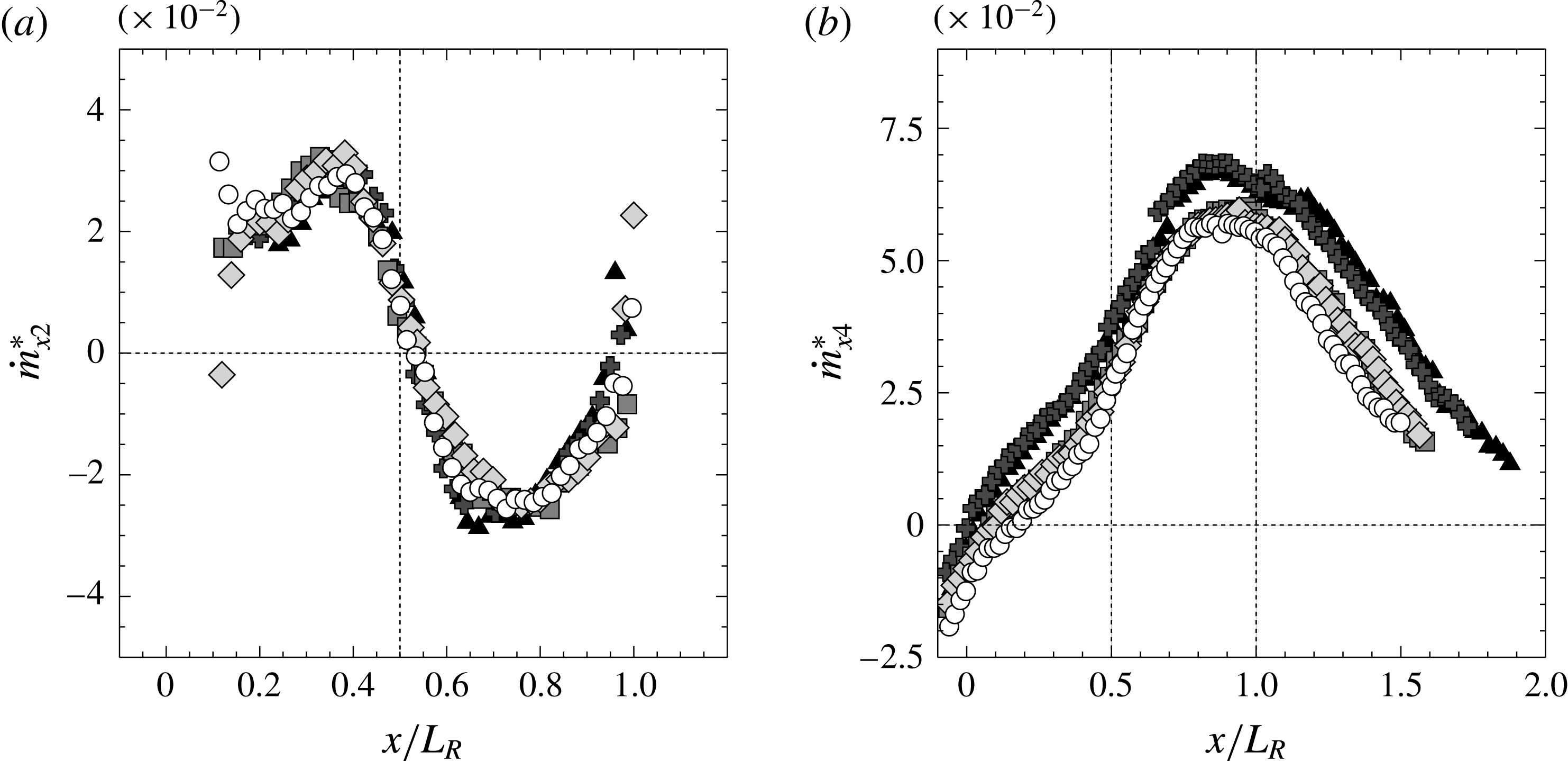
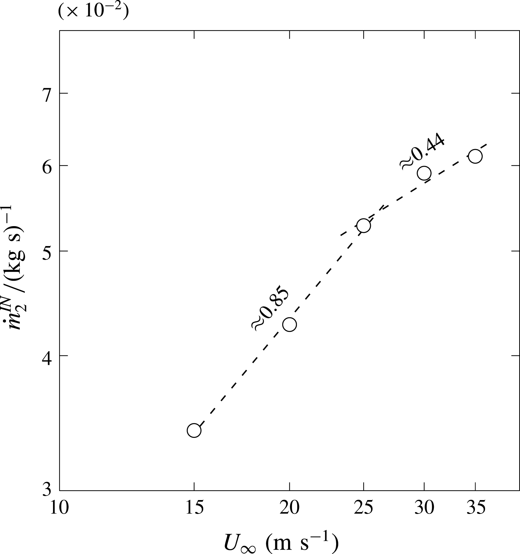
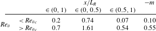
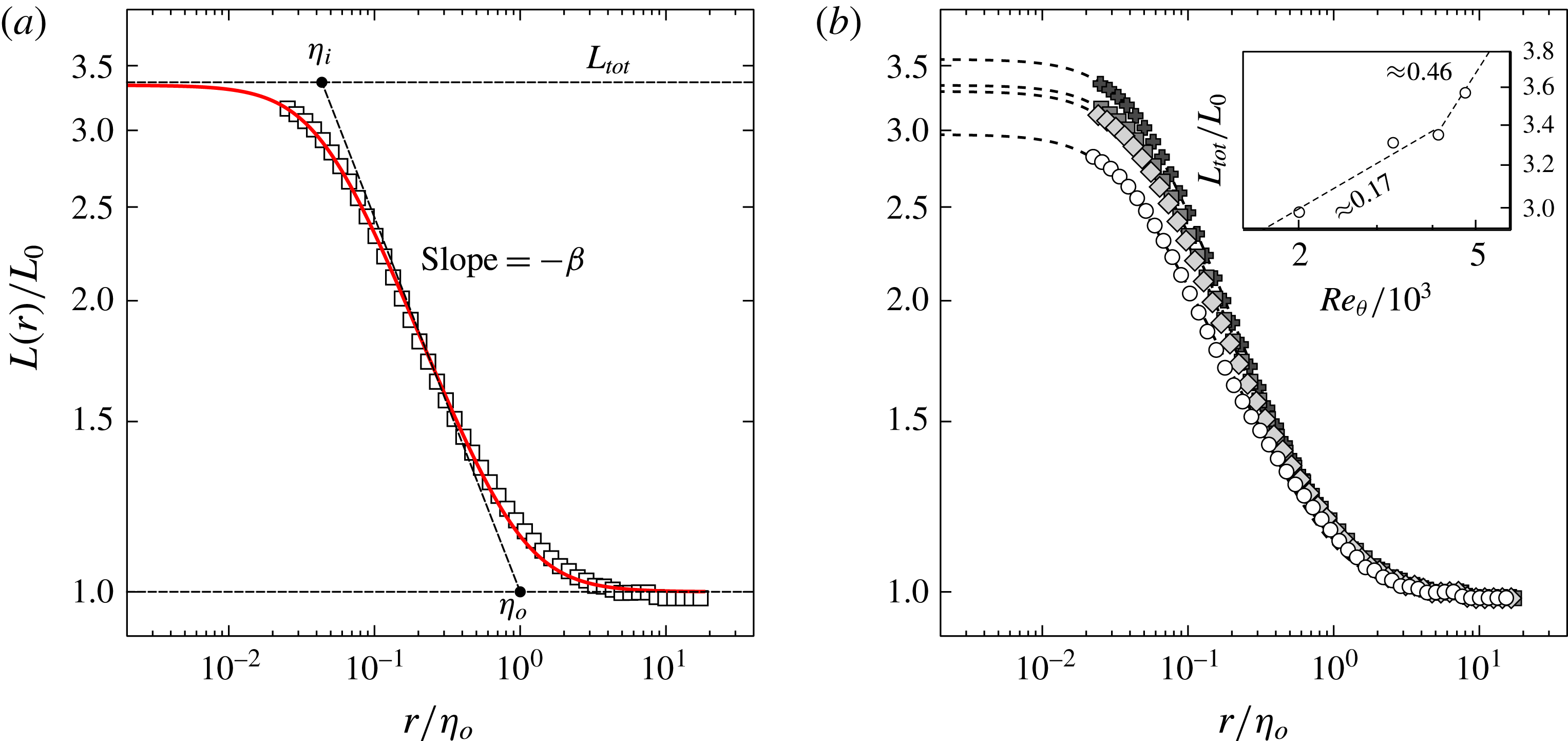
1 Introduction
Separating/reattaching flows are of primary importance in a number of industrial applications, encompassing bluff bodies such as ground vehicles, streamlined bodies such as wings and blades at high incidence/pitch angle, combustion chambers, turbines and pipelines. In most of these applications, flow separation leads to detrimental effects such as losses of aerodynamic performances (drag increase, lift decrease or both) or intense unsteady structural loads eventually leading to accelerated structural fatigue. This means that flow separation prevents the use of these systems at their nominal operating conditions. To mitigate its effects, over the past decades great attention has been paid to prediction of flow separation and its control. Anyway, research encountered a number of complex issues. On one hand, most industrial applications feature very large Reynolds numbers, seldom reachable to fully resolved simulations, i.e. direct numerical simulations (DNS), or even filtered simulations as large-eddy simulations (LES). This implies that simulations based on Reynolds-averaged Navier–Stokes (RANS) equations remain the main vector to design these systems. It is well known, however, that turbulence transport models used in RANS are not relevant to accurately predict separating/reattaching flows even in simple geometries (see e.g. Garnier et al. Reference Garnier, Pamart, Dandois and Sagaut2012). On the other hand, knowledge of the scaling parameters of separating/reattaching flows is essential to design efficient control systems and to ensure scalability from laboratory to full-scale applications. Indeed, even for black box approaches, the effectiveness of a control loop will depend on how well design parameters (e.g. sensor/actuator choice and location) match flow parameters (e.g. natural frequency, sensitive regions). However, flow separation induces complex physical interactions between a broad range of time and length scales, making its modelling and understanding challenging issues which are usually addressed through time-consuming trial and error procedures. Fundamental investigations are then necessary to bring new insights on the physical mechanisms underlying separating/reattaching flows.
One of the main features of these flows is a separated shear layer, which originates from the separation of an incoming boundary layer. The separated shear layer grows and eventually hits the wall at the reattachment point, beyond which the flow relaxes to a new boundary layer (Le, Moin & Kim Reference Le, Moin and Kim1997). Due to their simple geometry and their widespread use in diffusers and bluff bodies, the backward-facing step (BFS) and descending ramps of various shapes have been used as prototypes of separating/reattaching flows. Generally speaking, these flows consist in an asymmetric, sudden or progressive expansion resulting in a strong adverse pressure gradient, which promotes separation. They present a large recirculation region and a rather straight separation line (Eaton & Johnston Reference Eaton and Johnston1981). The separation point may be fixed or sliding, depending if salient or rounded edges are used. Important efforts have also been dedicated to understanding the complex physics underlying separated shear layer development and reattachment, characterised by a wide range of time and length scales in mutual interplay. Eaton & Johnston (Reference Eaton and Johnston1981) and Le et al. (Reference Le, Moin and Kim1997) observed that in BFS at moderate Reynolds number (
 $Re$
) the reattachment point exhibits a low frequency flapping motion. The presence of the flapping motion was not observed in the DNS and LES performed by Dandois, Garnier & Sagaut (Reference Dandois, Garnier and Sagaut2007) over a rounded ramp. However, these authors reported the existence of a convective instability in the separated shear layer, which was used for purpose of active control design. At the same time, Le et al. (Reference Le, Moin and Kim1997) pointed out that turbulent production, transport and dissipation occurring at higher frequency/wavenumber ranges give significant contributions to the turbulent kinetic energy budget.
One important aspect highlighted by many of these works is the influence of shear layer entrainment on the behaviour of separating/reattaching flows. It is noted that the term entrainment will be used to address all possible mechanisms that are responsible for transfer of flow properties (scalar or vectorial) from one region of the flow to another, these regions being separated by an interface. Chapman, Kuehn & Larson (Reference Chapman, Kuehn and Larson1958) first suggested that downstream of a BFS the backflow must balance mass entrainment through the bottom edge of the separated shear layer. As such, shear layer entrainment has a direct impact on the recirculation length
 $L_{R}$
, i.e. the streamwise distance between the separation and reattachment point, as well as on the distribution of the pressure coefficient
 $C_{p}$
(see Adams & Johnston (Reference Adams and Johnston1988a
), Adams & Johnston (Reference Adams and Johnston1988b
) and references therein). In the framework of flow control it was shown that beneficial effects (e.g.
 $L_{R}$
reduction) are obtained by increasing entrainment into the shear layer (Sigurdson Reference Sigurdson1995 among others). This being so, Eaton & Johnston (Reference Eaton and Johnston1981), Adams & Johnston (Reference Adams and Johnston1988a
) and Simpson (Reference Simpson1989) reviewed the change of
 $L_{R}$
and
 $C_{p}$
distribution with parameters affecting the shear layer, such as incoming boundary layer thickness and state (i.e. laminar or turbulent),
 $Re$
or expansion ratio. To date, some dependencies of
 $L_{R}$
and
 $C_{p}$
distribution on these parameters have been evidenced, but a full understanding is still missing.
Most of the past works on separating/reattaching flows, and in particular BFS and ramps, focused on characteristics of the mean field (as
 $L_{R}$
or the
 $C_{p}$
distribution) or turbulence at large scale (Song & Eaton Reference Song and Eaton2003; Song & Eaton Reference Song and Eaton2004; Cherry, Elkins & Eaton Reference Cherry, Elkins and Eaton2008; Cuvier et al.
Reference Cuvier, Braud, Foucaut and Stanislas2011; Nadge & Govardhan Reference Nadge and Govardhan2014; Kourta, Thacker & Joussot Reference Kourta, Thacker and Joussot2015) with the purpose of assessing numerical modelling (Neumann & Wengle Reference Neumann and Wengle2003) and designing control (see McCormick Reference McCormick2000; Kumar & Alvi Reference Kumar and Alvi2005; Dandois et al.
Reference Dandois, Garnier and Sagaut2007; Joseph et al.
Reference Joseph, Stella, Mazellier and Kourta2016 among others). However, this macroscopic approach appears to be incomplete when applied to the investigation of entrainment. Indeed, the multiscale nature of the turbulent interfaces (and accordingly of the transfer mechanisms) through which entrainment takes place is known at least from the seminal work of Corrsin & Kistler (Reference Corrsin and Kistler1955), and has been confirmed and expressed in the framework of fractal theory by Sreenivasan & Meneveau (Reference Sreenivasan and Meneveau1986), Sreenivasan, Ramshankar & Meneveau (Reference Sreenivasan, Ramshankar and Meneveau1989), Meneveau & Sreenivasan (Reference Meneveau and Sreenivasan1990) and more recently by Thiesset et al. (Reference Thiesset, Maurice, Halter, Mazellier, Chauveau and Gökalp2016) among others. Corrsin & Kistler (Reference Corrsin and Kistler1955) interpreted turbulent entrainment fundamentally as a small-scale, viscous phenomenon, which nibbles bites of irrotational fluid into turbulence. Corrsin & Kistler (Reference Corrsin and Kistler1955) theorised that such nibbling mechanism is driven by jumps in the vorticity and velocity fields, that take place at the so-called turbulent/non-turbulent interface (TNTI), on velocity and length scales that are of the order of the smallest scales of the flow (the so-called viscous superlayer). This vision was at first questioned by experimental studies carried out during the 1970s, that seemed to show that turbulent entrainment is rather dominated by large structures, which engulf large chunks of irrotational fluid into the turbulent bulk of the flow (Brown & Roshko Reference Brown and Roshko1974). During the last decades, the development of efficient image-based techniques (e.g. planar laser induced fluorescence (PLIF) and particle image velocimetry (PIV)) and the increased availability of DNS have given access to large portions of the TNTI and of the neighbouring velocity and vorticity fields, paving the way to finer assessment of fluxes through the TNTI. These new measurements confirmed the existence of a viscous superlayer and showed that small scales are responsible for most of mass transfer through the TNTI (see for instance Westerweel et al.
Reference Westerweel, Fukushima, Pedersen and Hunt2005; Westerweel et al.
Reference Westerweel, Fukushima, Pedersen and Hunt2009; da Silva & Taveira Reference da Silva and Taveira2010). However, it was also found that nibbling is poorly correlated to small-scale turbulence (Holzner & Lüthi Reference Holzner and Lüthi2011) and that large scales do influence global entrainment (Bisset, Hunt & Rogers Reference Bisset, Hunt and Rogers2002; Krug et al.
Reference Krug, Holzner, Lüthi, Wolf, Kinzelbach and Tsinober2015). Using time-resolved PLIF, Mistry et al. (Reference Mistry, Philip, Dawson and Marusic2016) showed recently that, given a coarse-grain filter of size
 $\unicode[STIX]{x1D6E5}$
, the mean mass flux through the TNTI of a turbulent jet is independent of
 $\unicode[STIX]{x1D6E5}$
, since the fractal scaling of interface length
 $L(\unicode[STIX]{x1D6E5})$
is compensated by the scaling of
 $\boldsymbol{v}_{\boldsymbol{E}}(\unicode[STIX]{x1D6E5})$
, the corresponding mean entrainment velocity (i.e. the velocity of the fluid relative to the interface). This confirmed the predictions of Meneveau & Sreenivasan (Reference Meneveau and Sreenivasan1990) and gave support to the idea that turbulent entrainment is a multiscale phenomenon, with the local viscous transfer (nibbling) adapting to the global entrainment rate imposed by large scales, i.e.
 $$\begin{eqnarray}\boldsymbol{v}_{\boldsymbol{E}}^{\unicode[STIX]{x1D708}}L^{\unicode[STIX]{x1D708}}=\boldsymbol{v}_{\boldsymbol{ E}}(\unicode[STIX]{x1D6E5})L(\unicode[STIX]{x1D6E5})=\boldsymbol{v}_{\boldsymbol{E}}^{A}L^{A},\end{eqnarray}$$
where the symbols
 $^{\unicode[STIX]{x1D708}}$
and
 $^{A}$
indicate quantities respectively involved in nibbling and large-scale entrainment. The formulation expressed in (1.1) has great implications in the design of control systems for separating/reattaching flows. Indeed, it suggests that strategies targeting either small-scale forcing (dissipation range) or large-scale forcing (production range) can both achieve entrainment modification. The former approach implies high frequency/low energy forcing, whereas low frequency/high energy forcing is required for the latter. Wiltse & Glezer (Reference Wiltse and Glezer1993) deployed direct small-scale excitation by means of piezoelectric actuators to control the shear layer of a jet. The excitation frequency was tuned to one order of magnitude lower than the convection frequency of the Kolmogorov scale, but was much larger than the natural roll-off frequency of the shear layer. This control strategy was able to alter significantly the entire cascade transfer of energy, while keeping the mean flow unchanged. Dandois et al. (Reference Dandois, Garnier and Sagaut2007) investigated the effect of control frequency of a synthetic jet on the separation over a rounded ramp. Two reduced frequencies were tested, each of these operating conditions leading to a strong modification of the recirculation length, which was reduced at low frequency forcing but increased at high frequency forcing.
This study aims at providing new insights on the physical mechanisms governing the development of the separating/reattaching flows. To our knowledge, no attempt has yet been undertaken to study the influence on turbulent entrainment of the full range of length scales that exists in these flows. This is the main goal of this work, which gives a specific emphasis to mass entrainment. The motivation of this study is twofold: (i) performing an investigation of mass entrainment through the separated shear layer that develops over a descending ramp; (ii) identifying the scaling parameters that drive mass entrainment at both large and small scales. To this purpose, a first issue to be addressed relates to the choice of the boundaries through which entrainment will be estimated. Among other options, the choice was made of analysing the TNTI and the separation line, which will hereafter be called recirculation region interface (RRI) for consistency. The TNTI lies between the free flow and the sheared region. Since the flow outside of the TNTI is unperturbed, in a way the TNTI can be considered as the upper boundary of the shear layer. The RRI, instead, wraps the backflow region, i.e. it separates positive mean streamwise velocities from negative ones. The RRI is the set of points where the streamwise velocity is zero (Simpson Reference Simpson1989), and as such it is not, rigorously speaking, a boundary of the shear layer (see for example the definitions of shear layer thickness by Dandois et al. (Reference Dandois, Garnier and Sagaut2007)). However, the analysis of the RRI seems of fundamental importance, as the RRI is representative of shear layer reattachment: let us remind the reader that the mean RRI is commonly used to determine
 $L_{R}$
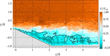
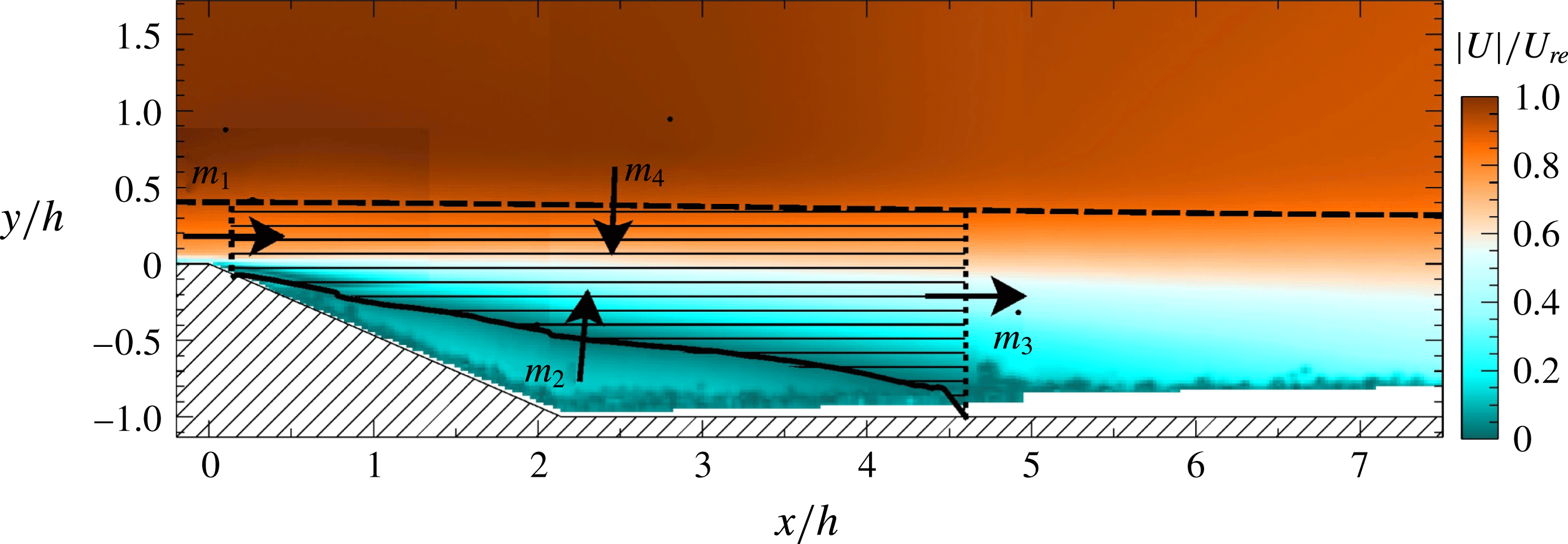
. Even if the behaviour of the interface has not been thoroughly studied, the RRI is nothing more than a constant-velocity line and as such it falls in the definitions of turbulent surfaces given by Pope (Reference Pope1988). It is then expected that the RRI will share the salient characteristics of other turbulent surfaces, such as the TNTI, in particular a multiscale nature and a role in entrainment. The relevance of these boundaries is emphasised in figure 1, which displays a typical velocity field measured with PIV (see §§ 2 and 3 for more details). The TNTI and the RRI are plotted in dashed and solid lines, respectively. It appears that these interfaces approximate the boundaries of the separated shear layer well. Furthermore, the multiscale nature of interface wrinkling is evident.
Instantaneous streamwise velocity field over the descending ramp. —— Instantaneous RRI. - - - Instantaneous TNTI.

A second problem tackled by the present study concerns the identification of those flow parameters that scale the separation/reattachment mechanisms in general and entrainment in particular. This is an important issue, since a thorough understanding of the factors that shape these flows might provide the elements for a model-based predictive approach for separating/reattaching flows, which would be mandatory for improving the reliability of model-based numerical simulations and the design of control systems as well. The present work contributes to this effort by studying the influence of a set of scaling parameters, including dimensionless incoming boundary layer thickness (
 $\unicode[STIX]{x1D6FF}/h$
), Reynolds number based on geometry (
 $Re_{h}$
) and Reynolds number of the incoming boundary layer (
 $Re_{\unicode[STIX]{x1D703}}$
). To expand the investigation, when possible the database reported in Kourta et al. (Reference Kourta, Thacker and Joussot2015) is also taken into account.
Finally, we attempt a qualitative assessment of the full range of length scales that exists in separating/reattaching flow. Since it has been observed that the largest and the smallest scales that wrinkle a turbulent interface (viz. the TNTI) are representative of the range of scales contained in the entire flow (Sreenivasan & Meneveau Reference Sreenivasan and Meneveau1986; da Silva & Pereira Reference da Silva and Pereira2008; de Silva et al. Reference de Silva, Philip, Chauhan, Meneveau and Marusic2013; Chauhan et al. Reference Chauhan, Philip, de Silva, Hutchins and Marusic2014). A scale-by-scale analysis of the turbulent interfaces might provide this kind of insight.
The paper is structured as follows: § 2 introduces the experimental set-up; § 3 investigates the main characteristics of the separated flow; § 4 studies the scaling parameters of large-scale features of the flow; § 5 explains how the TNTI is detected from PIV fields; global and local mean mass fluxes through the two interfaces are investigated in § 6; § 7 provides a discussion of implications at small scale; a summary and conclusions are given in § 8.
2 Experimental set-up
2.1 Test section and model details
Experiments were performed in the subsonic Eiffel wind tunnel of PRISME Laboratory, at University of Orléans, France. The facility has a
 $2~\text{m}$
long test section with a square cross-section of width
 $w=0.5~\text{m}$
, preceded by a settling chamber connected to the test section by a 16 : 1 contraction. It can reach a maximum free-stream velocity of
 $50~\text{m}~\text{s}^{-1}$
, with residual turbulence intensity of
 $0.5\,\%$
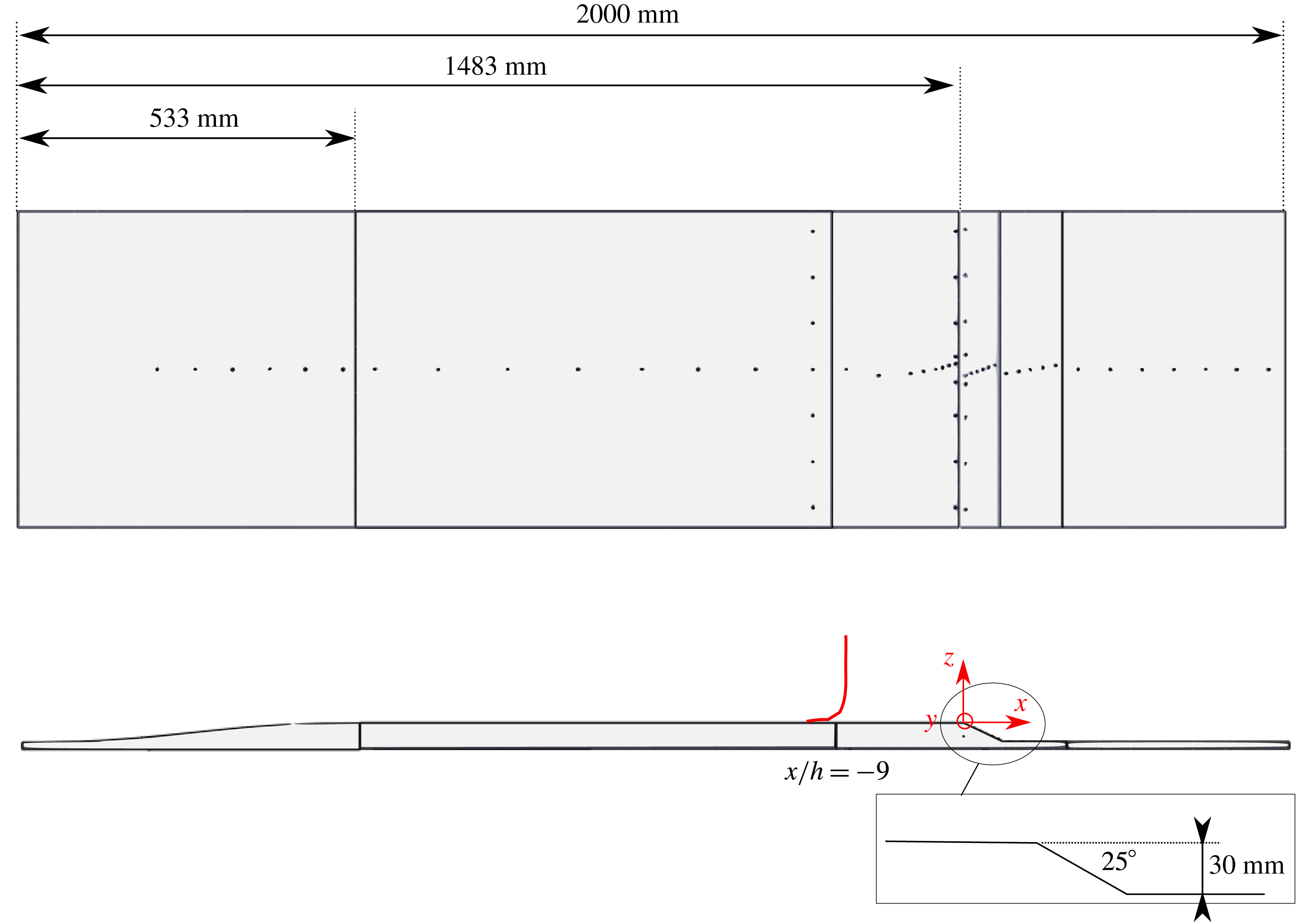
. The experimental model (figure 2) on which separation/reattachment occurs is composed of four parts: (i) a fifth-order polynomial contraction (Bell & Mehta Reference Bell and Mehta1988; Brassard & Ferchichi Reference Brassard and Ferchichi2005); (ii) a flat plate where turbulent boundary layer grows; (iii) a descending ramp of slope
 $\unicode[STIX]{x1D6FC}=25^{\circ }$
, with salient edge and step height
 $h=30~\text{mm}$
. The resulting expansion ratio
 $ER=w/(w-h)$
is equal to 1.064; (iv) a second flat plate on which the flow relaxes. The aspect ratio
 $w/h$
is approximately 17, which guarantees that the mean flow is quasi-bidimensional (see Eaton & Johnston Reference Eaton and Johnston1981 and § 3.3). We define the Cartesian coordinate system (
 $X;Y;Z$
), centred at midspan on the upper ramp edge (see figure 2). Following the suggestions of Kourta et al. (Reference Kourta, Thacker and Joussot2015), transition of the boundary layer was triggered with a zigzag tripper of height
 $0.5~\text{mm}$
, placed at
 $x/h\approx -48.5$
. The model replaced the floor of the test section, so that the junctions with the convergent and the diffuser of the wind tunnel were smooth. The reference free-stream velocity
 $U_{ref}$
and free-stream pressure
 $p_{ref}$
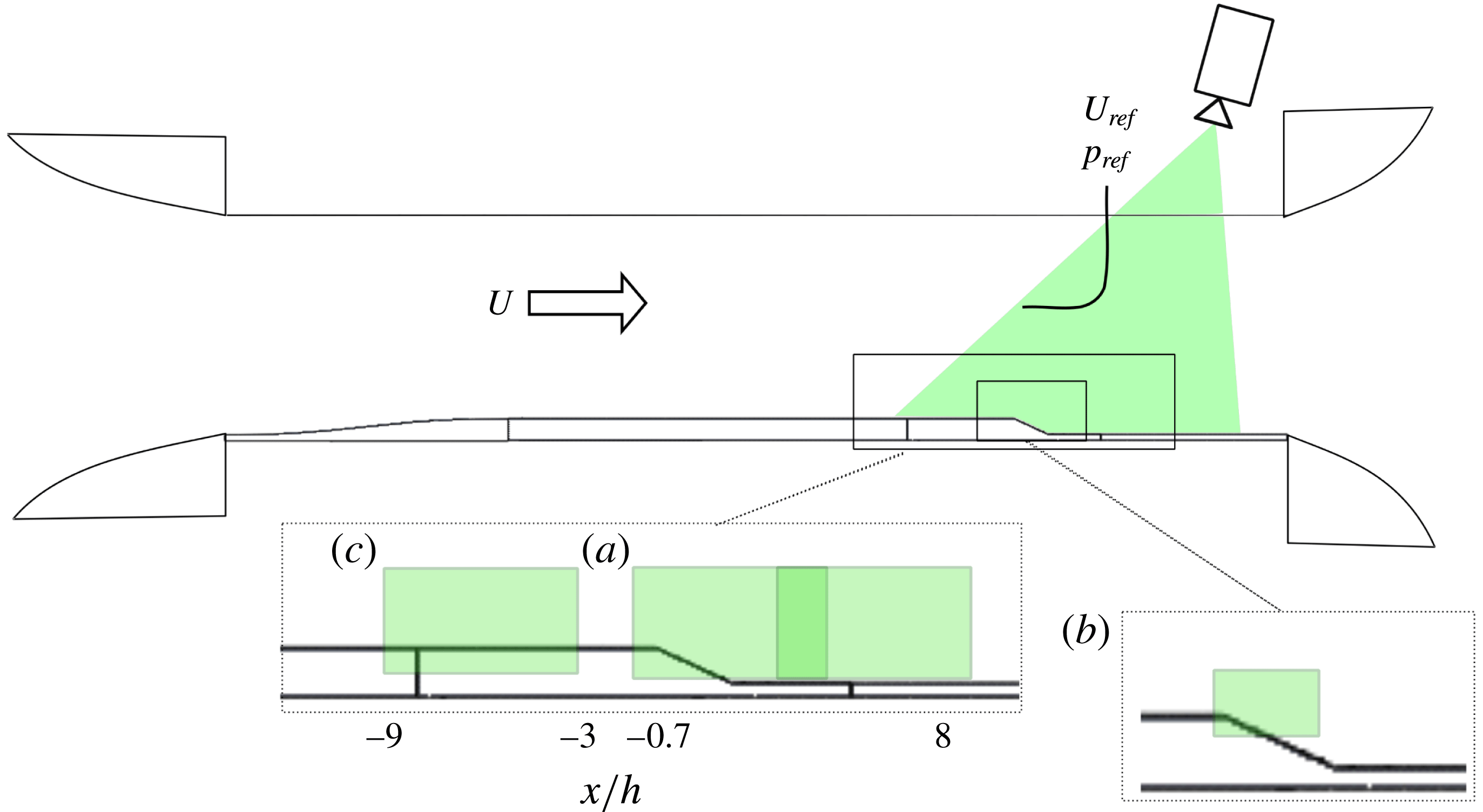
were measured with a Pitot tube (see figure 3) placed at midspan, above the upper edge of the ramp (
 $x/h=0$
;
 $y/h=0$
;
 $z/h=9$
). Five values of
 $U_{ref}$
were tested, ranging from
 $U_{ref}=15~\text{m}~\text{s}^{-1}$
to
 $U_{ref}=35~\text{m}~\text{s}^{-1}$
. One straightforward choice for a parameter of similitude is the Reynolds number based on step height
 $Re_{h}=U_{ref}h/\unicode[STIX]{x1D708}$
, where
 $\unicode[STIX]{x1D708}=1.5\times 10^{-5}~\text{m}^{2}~\text{s}^{-1}$
is the kinematic viscosity for air. In a way,
 $Re_{h}$
relates viscous scales to the scale of the macroscopic forcing of the flow. Table 1 lists the values of
 $Re_{h}$
for all tested velocities.
Dimensions of the experimental model. Dots represent pressure taps. The boundary layer measured at
 $x/h=-9$
(red line) is used as a reference for scaling parameters.

Integration of the experimental model into the wind tunnel and PIV set-ups. Letters indicate the three PIV fields. (a) Large field; (b) detailed field; (c) auxiliary field.

Boundary layer properties, measured at the reference section
 $x/h=-9$
. The full boundary layer thickness
 $\unicode[STIX]{x1D6FF}$
and the friction velocity
 $u_{\unicode[STIX]{x1D70F}}$
are obtained with the composite profile of Chauhan, Monkewitz & Nagib (Reference Chauhan, Monkewitz and Nagib2009). It is
 $Re_{h}=U_{\infty }h/\unicode[STIX]{x1D708}$
,
 $Re_{\unicode[STIX]{x1D6FF}_{1}}=U_{\infty }\unicode[STIX]{x1D6FF}_{1}/\unicode[STIX]{x1D708}$
,
 $Re_{\unicode[STIX]{x1D703}}=U_{\infty }\unicode[STIX]{x1D703}/\unicode[STIX]{x1D708}$
and
 $Re_{\unicode[STIX]{x1D70F}}=\unicode[STIX]{x1D6FF}u_{\unicode[STIX]{x1D70F}}/\unicode[STIX]{x1D708}$
.
 $H_{12}$
is the shape factor (
 $\equiv \unicode[STIX]{x1D6FF}_{1}/\unicode[STIX]{x1D703}$
). The Kolmogorov length scale,
 $\unicode[STIX]{x1D702}$
, is estimated at the height from the wall where the mean TNTI is located.

2.2 Measurement devices
2.2.1 Boundary layer measurements
Since it provides the initial conditions from which the massive separation onsets, it is mandatory to characterise the boundary layer developing upstream of the upper edge of the ramp. In this respect, one important concern is the choice of a suitable streamwise reference position where boundary layer properties are assessed. One straightforward option is a close neighbourhood of
 $x/h=0$
, but this region has the drawback of being affected by the pressure gradient induced by geometry. This increases the probability of having boundary layer velocity profiles that diverge from the canonical forms and are hence difficult to compare from flow to flow. The obvious alternative is to place the reference section upstream. This choice might be promising, because there is evidence that some degree of correlation exists between the properties of a separating/reattaching flow and those of the boundary layer much upstream of the separation point. For example, Neumann & Wengle (Reference Neumann and Wengle2003) reported that a passive actuator is most effective at reducing the recirculation region of a BFS flow when it is placed at least at
 $x/h=-4$
. It is clear that this point is of extreme interest for separation control, because it might provide premise for synthesis of feed-forward control systems based on upstream boundary layer measurements. As so, the reference section was placed at
 $x/h\approx -9$
. At this position the sizing criterion of Neumann & Wengle (Reference Neumann and Wengle2003) is satisfied and wall pressure gradient approaches zero (see § 3). At the same time, the scaling laws of pressure distribution (see § 3.3) seem to still hold, which is no longer true for more upstream positions.
Measurements were performed with a single component hot-wire (Dantec 55P15 probe) driven in constant-temperature mode at an overheat factor of 1.25 by a Dantec Streamware 90N10 Frame. The probe was calibrated with a fourth-order polynomial and compensated for temperature drift. Probe calibration was repeated once every 2 h. Spatial resolution can be assessed as
 $\ell _{w}/\unicode[STIX]{x1D706}_{m}$
. Here
 $\ell _{w}$
is the sensing length (
 $1.25~\text{mm}$
) and
 $\unicode[STIX]{x1D706}_{m}$
is the characteristic length scale of the two-point velocity correlation along the length of the wire, as discussed by Philip et al. (Reference Philip, Hutchins, Monty and Marusic2013). According to these authors, one can put
 $\unicode[STIX]{x1D706}_{m}=0.2\unicode[STIX]{x1D6FF}$
for
 $y/\unicode[STIX]{x1D6FF}>0.5$
, where
 $\unicode[STIX]{x1D6FF}$
is the boundary layer thickness. This yields
 $\ell _{w}/\unicode[STIX]{x1D706}_{m}\approx 0.20$
to
 $0.25$
, suggesting that hot-wire resolution should be sufficient to study the flow at the location of the mean TNTI (see § 5). However, close to the wall it is
 $\ell _{w}/\unicode[STIX]{x1D706}_{m}\sim \ell _{w}^{+}$
, where
 $\ell _{w}$
is normalised with inner scales, i.e.
 $\unicode[STIX]{x1D708}$
and friction velocity
 $u_{\unicode[STIX]{x1D70F}}$
. Depending on
 $Re$
, it is
 $\ell _{w}/\unicode[STIX]{x1D706}_{m}\approx 55$
to
 $105$
. Strong attenuation of streamwise fluctuations is then to be expected in proximity of the wall, as shown in § 3.1. For each measurement point, samples were acquired at a rate of 20 kHz for about 13 s. To avoid aliasing, the signals were filtered with a low-pass analogue filter with a cutoff frequency
 $f_{c}$
set at 10 kHz, which ranged from 0.22 to 0.62 times the convective frequency
 $f_{\unicode[STIX]{x1D702}}=U_{ref}/(2\unicode[STIX]{x03C0}\unicode[STIX]{x1D702})$
(Mazellier & Vassilicos Reference Mazellier and Vassilicos2010), which relates transport of the smallest structures of the flow past a measurement point. In this latter expression,
 $\unicode[STIX]{x1D702}=\left(\unicode[STIX]{x1D708}^{3}/\unicode[STIX]{x1D716}\right)^{1/4}$
is the Kolmogorov length scale, evaluated at the mean location of the TNTI (see § 5). The dissipation rate
 $\unicode[STIX]{x1D716}$
is estimated under the hypothesis of local isotropy, using the surrogate relation
 $\unicode[STIX]{x1D716}=15\unicode[STIX]{x1D708}\langle \left(\unicode[STIX]{x2202}u^{\prime }/\unicode[STIX]{x2202}x\right)^{2}\rangle$
, where
 $u^{\prime }$
is the fluctuating streamwise velocity. According to the so-called Reynolds decomposition, it is
 $u^{\prime }=u-U$
, where
 $u$
and
 $U$
are the instantaneous and mean streamwise velocities. In the following, the same decomposition and notation apply to the wall-normal velocity component
 $v$
. In the expression for
 $\unicode[STIX]{x1D716}$
, Taylor’s hypothesis is invoked to reconstruct the space derivative of
 $u^{\prime }$
from its time derivative. The value of
 $\unicode[STIX]{x1D702}$
is reported in table 1 for each
 $Re$
.
2.2.2 Wall pressure measurements
Streamwise and spanwise wall pressure distributions were investigated with a total of 64 static pressure taps, connected to 2 pressure scanners (
 $\unicode[STIX]{x1D707}$
DAQ-32C models manufactured by Chell Instruments) that were interfaced and multiplexed with an acquisition unit. Pneumatic connections were provided by 1 m long vinyl tubes of inner diameter equal to 1.25 mm. According to manufacturer specifications, pressure measurement uncertainty is smaller than 6 Pa. The model was fitted with 38 pressure taps in the streamwise direction (figure 2). The spatial resolution was finer in the neighbourhood of the edges of the ramp. Flow homogeneity in the spanwise direction was assessed along 3 rows of pressure taps, respectively located at
 $x/h=-7.67$
(6 pressure taps),
 $-0.17$
(8 pressure taps) and 0.36 (8 pressure taps). Note that the length of pneumatic connections avoids any reliable analysis of pressure fluctuations. For more details about the frequency response of our pressure measurement system, the reader is referred to Kourta et al. (Reference Kourta, Thacker and Joussot2015). Accordingly, only mean pressure distributions were computed, using
 $3\times 10^{4}$
samples acquired over about 50 s. This represents between
 $2.5\times 10^{4}$
and
 $6\times 10^{4}$
characteristic time scales
 $h/U_{ref}$
, which was sufficient for statistical convergence.
2.2.3 Velocity field measurements
PIV is the main measurement technique used in this work, because it allows us to study the development of the shear layer on conspicuous portions of the flow. Admittedly, PIV (as most other planar imaging techniques) only resolves two components of the velocity field and only gives access to the azimuthal component of vorticity. This is an important drawback when studying turbulence, which is intrinsically three-dimensional. This limitation should not however impact the analysis of the mean field (see § 6) too much, since the spanwise pressure distribution demonstrates that the latter is almost bidimensional (§ 3.3). Bias could be stronger when considering the smallest turbulent length scales resolved by the PIV (e.g. when investigating entrainment through instantaneous interfaces in § 7), since the third velocity component might become quantitatively relevant as turbulence approaches (assumed) isotropy. Although this issue is not solved in this study, it is hoped that the bidimensional analysis allowed by PIV data will also be qualitatively representative of entrainment in the spanwise direction. In this respect, the results reported by Veynante et al. (Reference Veynante, Lodato, Domingo, Vervisch and Hawkes2010) are encouraging. These authors verified that properties of turbulent flames (viz. flame wrinkling) in the unresolved direction can be modelled from planar measurements, with very good agreement with DNS.
Particle images were captured with a LaVision VC-Imager camera (
 $4032\times 2688$
pixels), synchronised with a double pulse, monochromatic Nd:Yag laser (wavelength 532 nm, rated
 $2\times 200$
mJ). The PIV plane was placed at
 $y/h\approx -1$
. Large-scale velocity fields were obtained with a Zeiss
 $50~\text{mm}$
ZF Makro Planar T* lens, which provided a camera resolution of
 $78~\unicode[STIX]{x03BC}\text{m}~\text{px}^{-1}$
and an exploitable field of view of
 $6h\times 2.5h$
. Three sections of the flow were successively investigated with these settings, respectively centred at
 $x/h\approx -6$
,
 $x/h\approx 2.5$
and
 $x/h\approx 5.5$
(figure 3). Statistics from the last two sections were merged into a single large field of approximately
 $9h\times 2.5h$
, which covers the entire recirculation region. The first field, instead, provided a set of PIV images of the incoming boundary layer: it will be referred to as the auxiliary field. In addition to these measurements, a
 $200~\text{mm}$
Nikon ED AF Micro Nikkor lens was used to investigate small-scale TNTI features on a detailed field, placed in the neighbourhood of the upper edge of the ramp (figure 3, field b). In this latter case, camera resolution was approximately 12
 $\unicode[STIX]{x03BC}\text{m}$
 $\text{px}^{-1}$
on an exploitable field of view of
 $1.5h\times 1.2h$
.
The flow was seeded with olive oil droplets of mean diameter
 $d_{p}=$
1
 $\unicode[STIX]{x03BC}\text{m}$
(according to the specifications of the aerosol generator). The Stokes number of the seeded flow was then
 $Sk=\unicode[STIX]{x1D70F}_{p}/\unicode[STIX]{x1D70F}_{\unicode[STIX]{x1D702}}\approx 2.5\times 10^{-3}$
, where
 $\unicode[STIX]{x1D70F}_{p}$
is the characteristic time response of oil droplet (estimated at 2.75
 $\unicode[STIX]{x03BC}\text{s}$
following Kourta et al. (Reference Kourta, Thacker and Joussot2015)). As
 $Sk\ll 1$
, oil droplets should trace the flow accurately at all turbulent scales.
PIV measurements were carried out at each tested
 $Re_{h}$
on all fields. However, data from the detailed field at
 $Re_{h}=7\times 10^{4}$
were discarded during post-processing due to technical problems. For each
 $Re_{h}$
, 2000 image pairs were recorded at an acquisition rate of 2 Hz. Then, image pairs were correlated with the multipass, graphics processing unit (GPU) direct correlation algorithm of the LaVision Davis 8.3 software suite. The size of the interrogation window was progressively refined from
 $64\times 64~\text{px}^{2}$
to
 $16\times 16~\text{px}^{2}$
, in each case with 50 % overlapping. This yielded a spatial resolution
 $\unicode[STIX]{x1D6E5}/\unicode[STIX]{x1D702}\approx 20$
for both large and auxiliary fields,
 $\unicode[STIX]{x1D6E5}/\unicode[STIX]{x1D702}\approx 3$
for the detailed field, where the value of
 $\unicode[STIX]{x1D702}$
is the one estimated from hot-wire data in § 2.2.1. PIV signal noise was assessed by comparing the square root of the streamwise Reynolds stress
 $\sqrt{\langle (u^{\prime })^{2}\rangle }$
(the symbol
 $\langle \cdot \rangle$
standing for ensemble averaging) to the value of residual turbulence of the wind tunnel. It is found that
 $\sqrt{\langle (u^{\prime })^{2}\rangle }/U_{\infty }\approx$
1.5 % to 2 % (PIV), for a residual turbulence of about 0.5 % (hot-wire), where
 $U_{\infty }$
is the local free-stream velocity. This is comparable to PIV noise levels achieved in other works on turbulent interfaces. For example, de Silva et al. (Reference de Silva, Philip, Chauhan, Meneveau and Marusic2013) reported
 $\sqrt{\langle (u^{\prime })^{2}\rangle }/U_{\infty }\approx 1\,\%$
in the free flow, for a value of residual turbulence of approximately 0.2 %.
3 Flow characterisation
This section provides an overall description of the flow. When possible, comparison with other separating/reattaching flows is exploited. In this respect, the work of Kourta et al. (Reference Kourta, Thacker and Joussot2015) provides a particularly interesting reference. Although the experimental set-up and the characteristics of the wind tunnel are sizeably different, the shape of the ramp used in that study is identical to the present one and the expansion ratio is comparable (
 $ER=1.1$
). The main geometrical difference is step height, which is approximately 3 times higher (
 $h=100~\text{mm}$
) in the study of Kourta et al. (Reference Kourta, Thacker and Joussot2015). In addition, the results reported in Kourta et al. (Reference Kourta, Thacker and Joussot2015) indicate that boundary layer thickness measured at
 $x/h=-8.9$
, which is very close to the reference section adopted in the present study, is of the same order of magnitude than the one observed here.
3.1 Incoming boundary layer
Table 1 summarises the main properties of the incoming boundary layer for all available
 $Re_{h}$
.
 $Re_{\unicode[STIX]{x1D70F}}$
is computed as
 $\unicode[STIX]{x1D6FF}u_{\unicode[STIX]{x1D70F}}/\unicode[STIX]{x1D708}$
, where boundary layer thickness
 $\unicode[STIX]{x1D6FF}$
and friction velocity
 $u_{\unicode[STIX]{x1D70F}}$
were computed with the composite boundary layer profile proposed by Chauhan et al. (Reference Chauhan, Monkewitz and Nagib2009). The displacement thickness
 $\unicode[STIX]{x1D6FF}_{1}$
and the momentum thickness
 $\unicode[STIX]{x1D703}$
are classically defined as follows:
 $$\begin{eqnarray}\unicode[STIX]{x1D6FF}_{1}\left(x\right)=\int _{0}^{\infty }\left(1-\frac{U(x,y)}{U_{\infty }(x)}\right)\text{d}y,\end{eqnarray}$$
 $$\begin{eqnarray}\unicode[STIX]{x1D703}\left(x\right)=\int _{0}^{\infty }\frac{U(x,y)}{U_{\infty }(x)}\left(1-\frac{U(x,y)}{U_{\infty }(x)}\right)\text{d}y.\end{eqnarray}$$
 $Re_{\unicode[STIX]{x1D703}}$
are high enough to expect a fully turbulent boundary layer, with the possible exception of
 $Re_{\unicode[STIX]{x1D703}}=2006$
(
 $Re_{h}=3\times 10^{4}$
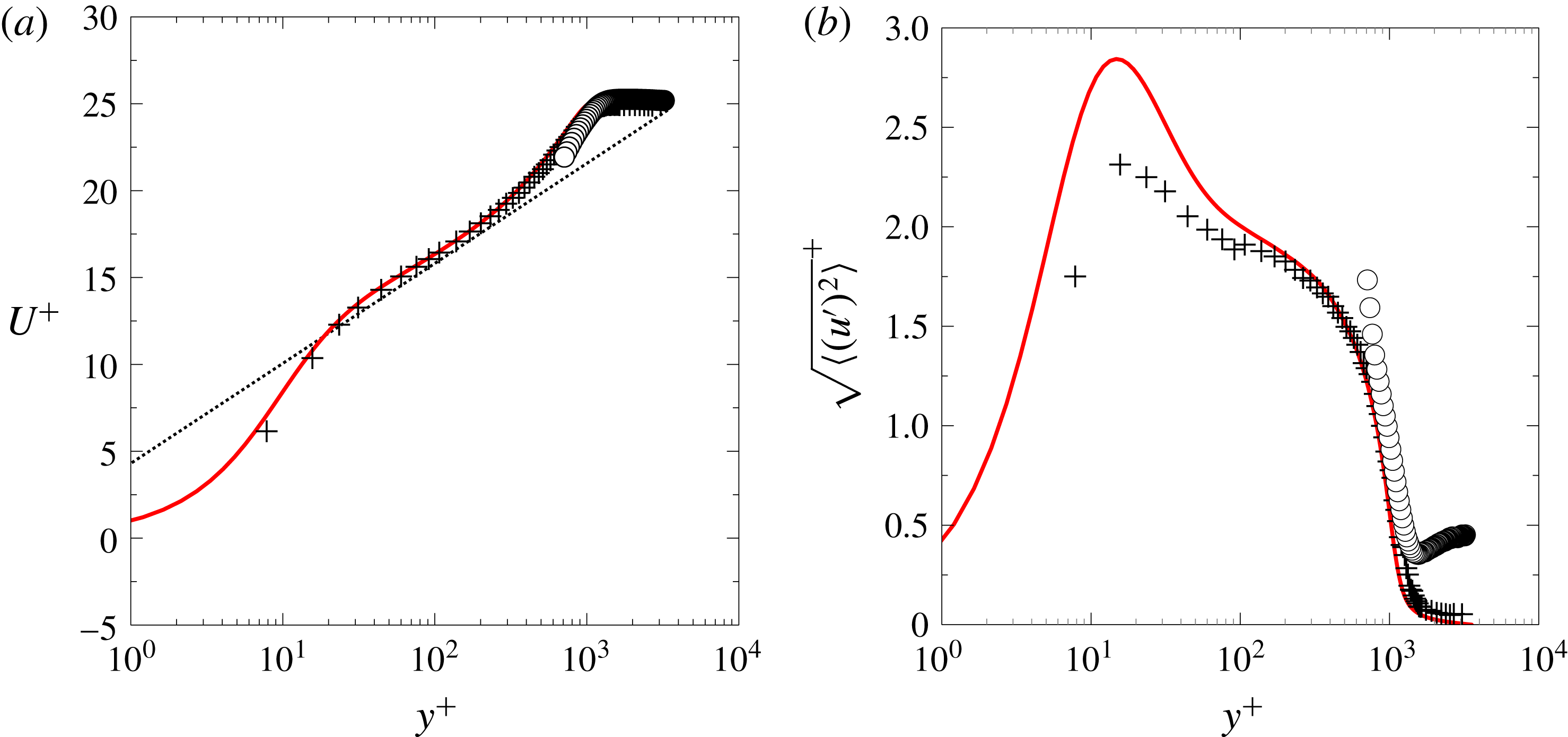
). To provide further insight into the state of the boundary layer, figure 4 presents the profiles of
 $U^{+}$
and of
 $\sqrt{\langle (u^{\prime })^{2}\rangle }^{\,+}$
, for the incoming boundary layer at
 $Re_{\unicode[STIX]{x1D70F}}\approx 1310$
(
 $Re_{h}=4\times 10^{4}$
,
 $Re_{\unicode[STIX]{x1D703}}=3262$
). Both curves are normalised with inner scales. For comparison purposes, the velocity profiles at
 $Re_{\unicode[STIX]{x1D70F}}=1043$
(
 $Re_{\unicode[STIX]{x1D703}}=3270$
) extracted from the DNS of a zero-pressure gradient (ZPG) boundary layer (Schlatter & Örlü Reference Schlatter and Örlü2010) are also reported. One can notice a fairly good agreement for
 $U^{+}$
, while
 $\sqrt{\langle (u^{\prime })^{2}\rangle }^{\,+}$
collapses well on the DNS for
 $y^{+}>100$
only. The strong attenuation of the inner peak of
 $\sqrt{\langle (u^{\prime })^{2}\rangle }^{\,+}$
may be mainly attributed to spatial integration over the sensing length of the hot-wire probe (see for example Wyngaard Reference Wyngaard1968; Ligrani & Bradshaw Reference Ligrani and Bradshaw1987; Örlü & Alfredsson Reference Örlü and Alfredsson2010; Philip et al.
Reference Philip, Hutchins, Monty and Marusic2013) but also to various effects such as pressure gradient and wall interferences. Since the RRI is not defined in the boundary layer and the TNTI is rather located in its outer region, probe resolution is good enough for the purposes of this work. Figure 4 also reports the boundary layer profiles computed from PIV data of the auxiliary field, at
 $Re_{h}=4\times 10^{4}$
. Due to wall reflections, data are exploitable only for
 $y^{+}>500$
, which corresponds approximately to
 $y/\unicode[STIX]{x1D6FF}>0.38$
. According to Chauhan et al. (Reference Chauhan, Philip, de Silva, Hutchins and Marusic2014), this extent is sufficient to cover almost the entire distribution of the TNTI.
Normalised boundary layer velocity profiles at
 $Re_{\unicode[STIX]{x1D70F}}=1310$
(
 $Re_{\unicode[STIX]{x1D703}}=3262$
). (a)
 $U^{+}$
; (b)
 $\sqrt{\langle (u^{\prime })^{2}\rangle }^{+}$
. + Hot-wire measurements at
 $x/h=-9$
;
 $\circ$
average along the PIV auxiliary field. —— (shown in red online) DNS at
 $Re_{\unicode[STIX]{x1D70F}}=1043$
(
 $Re_{\unicode[STIX]{x1D703}}=3270$
) as given in Schlatter & Örlü (Reference Schlatter and Örlü2010). - - - Log law,
 $\unicode[STIX]{x1D705}=0.39$
and
 $B=4.3$
(Marusic et al.
Reference Marusic, Monty, Hultmark and Smits2013).

Mean separated flow at
 $Re_{h}=5\times 10^{4}$
. - - - Mean TNTI. —— Mean RRI. The shaded area marks the control volume
 ${\mathcal{V}}_{c}$
.

Evolution of the recirculation length
 $L_{R}$
with
 $Re_{h}$
.

3.2 The separated shear layer
Figure 5 shows the mean separated flow for
 $Re_{h}=5\times 10^{4}$
. The separation of the incoming boundary layer is induced by the sharp expansion of the test section. Downstream of the separation point, the flow is marked by a large mean recirculation region where
 $U<0$
, which extends up to the reattachment point where the separated shear layer hits the wall. The RRI is the external boundary of the recirculation region. In this study, it is defined either by the isoline
 $U=0$
on the mean streamwise velocity field, or by the set of points where the backflow coefficient
 $\unicode[STIX]{x1D712}$
is equal to 0.5,
 $\unicode[STIX]{x1D712}$
being defined as the fraction of time that the flow moves downstream (Simpson Reference Simpson1989; Cuvier Reference Cuvier2012). The recirculation region is usually characterised by its length
 $L_{R}$
, which corresponds to the streamwise distance between the separation point (i.e. the first point of the RRI) and the reattachment point (i.e. the last point of the RRI). Although not shown here, topologies that are comparable to that displayed in figure 5 were observed for each
 $Re_{h}$
, the main difference being the location of the mean reattachment point, which moves upstream for increasing
 $Re_{h}$
. Based on PIV data, in this work the ratio
 $L_{R}/h$
ranges from 5.16 to 4.11 (table 2). This trend is consistent with data reported by Kourta et al. (Reference Kourta, Thacker and Joussot2015) and those observed in other massively separated turbulent flows, e.g. downstream of a backward-facing step (Eaton & Johnston Reference Eaton and Johnston1981). It seems important to stress that
 $L_{R}$
can be interpreted as the streamwise scale of shear layer development. The latter is often characterised with the streamwise evolution of either a generalised momentum thickness
 $\unicode[STIX]{x1D703}_{SL}$
or of the vorticity thickness
 $\unicode[STIX]{x1D6FF}_{\unicode[STIX]{x1D714}}$
. According to Dandois et al. (Reference Dandois, Garnier and Sagaut2007),
 $\unicode[STIX]{x1D703}_{SL}$
and
 $\unicode[STIX]{x1D6FF}_{\unicode[STIX]{x1D714}}$
are defined as follows:
 $$\begin{eqnarray}\unicode[STIX]{x1D703}_{SL}(x)=\int _{y_{min}}^{\infty }\!\frac{U(x,y)-U_{min}(x)}{U_{\infty }(x)-U_{min}(x)}\left(1-\frac{U(x,y)-U_{min}(x)}{U_{\infty }(x)-U_{min}(x)}\right)\text{d}y,\end{eqnarray}$$
 $$\begin{eqnarray}\unicode[STIX]{x1D6FF}_{\unicode[STIX]{x1D714}}(x)=\frac{U_{\infty }(x)-U_{min}(x)}{\left(\unicode[STIX]{x2202}U(x,y)/\unicode[STIX]{x2202}y\right)_{max}},\end{eqnarray}$$
 $U_{min}(x)$
is a local minimum streamwise velocity. Figure 6 shows clearly that
 $L_{R}$
and
 $h$
are appropriate scaling parameters for both
 $\unicode[STIX]{x1D703}_{SL}$
and
 $\unicode[STIX]{x1D6FF}_{\unicode[STIX]{x1D714}}$
. In principle, the development of the shear layer may be governed by at least two factors: entrainment of external fluid, that drives the spreading rate of free shear layers (see Pope Reference Pope2000) and
 $ER$
. Adams & Johnston (Reference Adams and Johnston1988a
) show that for high values of
 $\unicode[STIX]{x1D6FF}/h$
the influence of
 $ER$
is sizeable at shear layer reattachment. To have some insights into the relative weight of these two mechanisms, let us consider spreading rates typical of free turbulent mixing layers, modelled by Browand & Troutt (Reference Browand and Troutt1985) as follows:
 $$\begin{eqnarray}\frac{\text{d}\unicode[STIX]{x1D703}_{SL}}{\text{d}x}=0.034\,\frac{U_{\infty }(x)-U_{min}(x)}{U_{\infty }(x)+U_{min}(x)},\end{eqnarray}$$
 $$\begin{eqnarray}\frac{\text{d}\unicode[STIX]{x1D6FF}_{\unicode[STIX]{x1D714}}}{\text{d}x}=0.17\,\frac{U_{\infty }(x)-U_{min}(x)}{U_{\infty }(x)+U_{min}(x)}.\end{eqnarray}$$
 $x/L_{R}<0.5$
, the velocity ratio in (3.3) ranges between 1.15 and 1.3. Then, equations (3.3) yield
 $\text{d}\unicode[STIX]{x1D703}_{SL}/\text{d}x\approx 0.042\pm 0.003$
and
 $\text{d}\unicode[STIX]{x1D6FF}_{\unicode[STIX]{x1D714}}/\text{d}x\approx 0.205\pm 0.015$
, compared to measured values of
 $0.05\pm 0.006$
and
 $0.22\pm 0.03$
, respectively. The relatively good agreement of estimated and observed values suggests that the separated shear layer behaves similarly to a free shear layer in a large region downstream of the upper edge of the ramp (Eaton & Johnston Reference Eaton and Johnston1981). This means that, in this region, the growth of the separated shear layer is dominated by entrainment. Interestingly, the growth rates of
 $\unicode[STIX]{x1D703}_{SL}/h$
and
 $\unicode[STIX]{x1D6FF}_{\unicode[STIX]{x1D714}}/h$
decrease for
 $x/L_{R}>0.5$
and (3.3) are no longer acceptable approximations. A similar slope change at a similar relative position was also observed by Dandois et al. (Reference Dandois, Garnier and Sagaut2007). Although the interactions between
 $ER$
and shear layer impingement at reattachment are complex (Adams & Johnston Reference Adams and Johnston1988a
), pressure data shown at § 3.3 illustrate that lower spreading rates are correlated with strong pressure recovery: this suggests that
 $ER$
might indeed play a role in the second half of the flow. However, entrainment appears to be the main contributor to spreading of the separated shear layer as a whole, since 75 % of total shear layer growth takes place within
 $x/L_{R}<0.5$
. Finally, provided that the TNTI and the RRI are well approximated by straight lines (see figure 5), it is easy to show that
 $L_{R}/h$
evolves as
 $(\text{d}\unicode[STIX]{x1D703}_{SL}/\text{d}x)^{-1}$
or
 $(\text{d}\unicode[STIX]{x1D6FF}_{\unicode[STIX]{x1D714}}/\text{d}x)^{-1}$
equivalently, i.e. the faster the separated shear layer grows, the smaller is the recirculation region (also see Adams & Johnston (Reference Adams and Johnston1988a
) on this matter). This is well supported by the inserts in figure 6.
Shear layer growth. (a) Generalised momentum thickness
 $\unicode[STIX]{x1D703}_{SL}$
; (b) vorticity thickness
 $\unicode[STIX]{x1D6FF}_{\unicode[STIX]{x1D714}}$
. Symbols: ○
 $Re_{h}=3\times 10^{4}$
;

 $Re_{h}=4\times 10^{4}$
;

 $Re_{h}=5\times 10^{4}$
;

 $Re_{h}=6\times 10^{4}$
; ▴
 $Re_{h}=7\times 10^{4}$
. The inserts show the
 $L_{R}$
dependency on shear layer growth rate. - - -
 $-1$
power law.

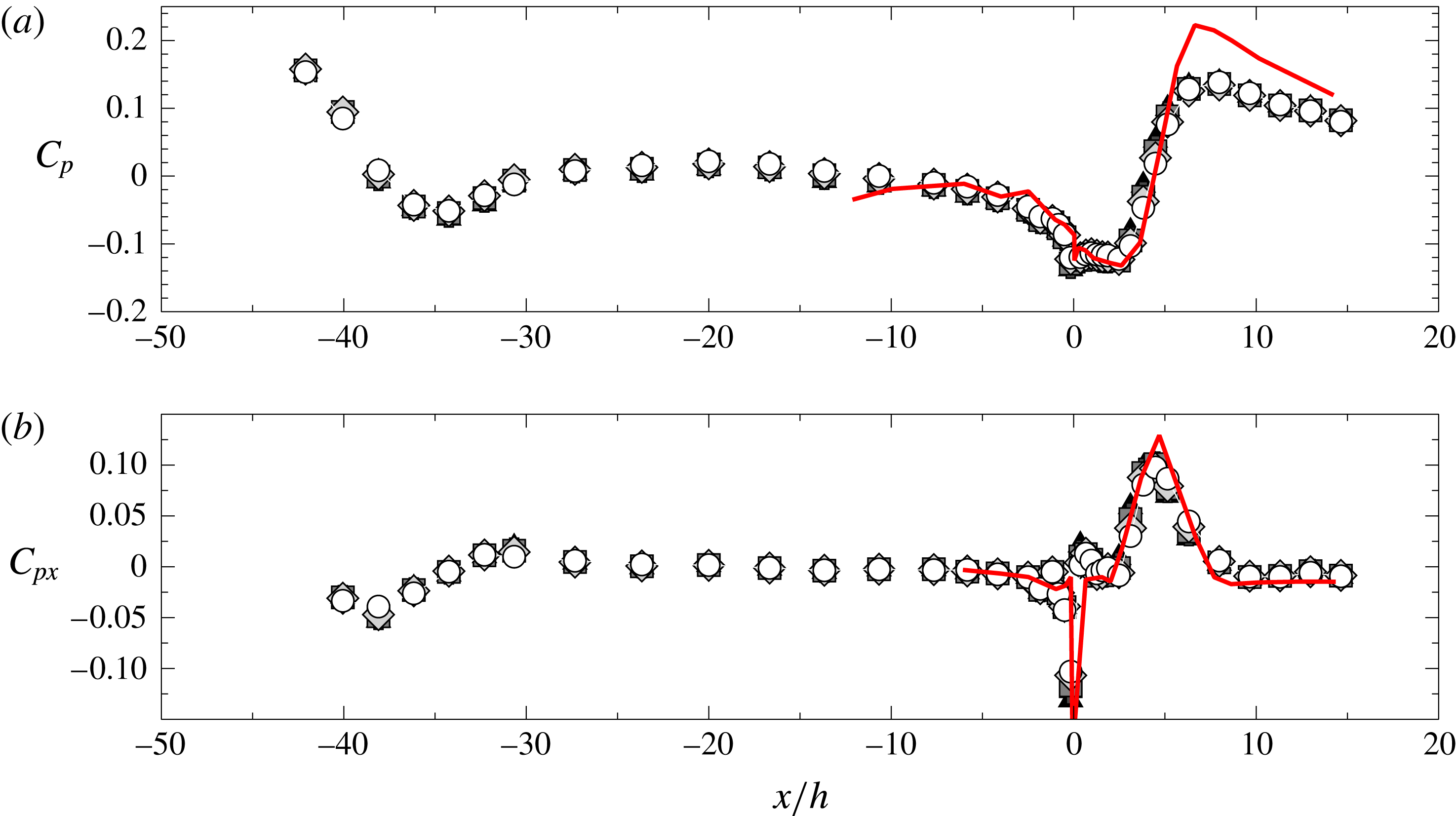
Streamwise evolution of (a) the pressure coefficient and (b) its dimensionless derivative. Symbols as in figure 6. —— (red online) Pressure data from Kourta et al. (Reference Kourta, Thacker and Joussot2015).

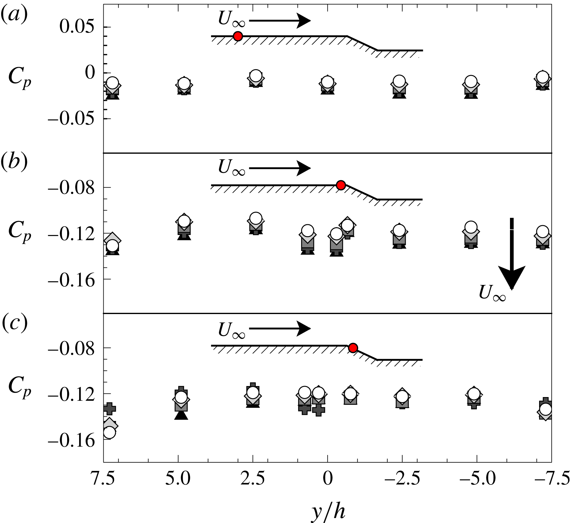
Spanwise pressure distributions. (a)
 $x/h=-7.67$
; (b)
 $x/h=-0.17$
; (c)
 $x/h=0.36$
. Symbols as in figure 6.

3.3 Wall pressure distribution
Separation has a direct effect on wall pressure distribution and accordingly on entrainment (see e.g. Eaton & Johnston Reference Eaton and Johnston1981). Figure 7 shows the streamwise evolution of the pressure coefficient
 $C_{p}$
, defined as follows:
 $$\begin{eqnarray}C_{p}=\frac{p-p_{ref}}{1/2\,\unicode[STIX]{x1D70C}\,U_{ref}^{2}},\end{eqnarray}$$
where
 $p$
is wall pressure. The streamwise coordinate is normalised on
 $h$
. The
 $C_{p}$
distribution appears to be a relatively weak function of
 $Re_{h}$
. Downstream of the contraction,
 $C_{p}$
stays roughly constant until the flow approaches the ramp. Although not perfectly zero, the dimensionless pressure gradient
 $C_{px}=h\,\text{d}C_{p}/\text{d}x$
in this region is small (figure 7
b), so that its influence on boundary layer development is assumed to be mild. The onset of separation at the upper edge of the ramp (
 $x/h=0$
) induces a strong decrease of pressure. The recirculation region is characterised by a low pressure plateau followed by a rapid pressure rise that reaches a maximum at
 $x/h\approx 7$
. In the following, the plateau and the peak
 $C_{p}$
values will be referred to as base
 $C_{p}$
(noted
 $C_{p,b}$
) and peak reattachment
 $C_{p}$
(noted
 $C_{p,r}$
), respectively. Spanwise pressure distributions (figure 8) confirm that the mean flow over the model is nearly bidimensional and that the mean separation is homogeneous at least over 60 % of tunnel width. Using
 $h$
to normalise the streamwise distance,
 $C_{p}$
and
 $C_{px}$
are in good agreement with Kourta et al. (Reference Kourta, Thacker and Joussot2015) in all those regions where the geometries of the two experiments are comparable, that is downstream of the separation point and over a large fraction of the flat plate upstream of the edge of the ramp (figure 7). This simply indicates that, for ramps with the same geometry, the pressure distribution approximately scales with step height. According to Adams & Johnston (Reference Adams and Johnston1988a
), the difference in observed
 $C_{p,r}$
can be explained by the different
 $\unicode[STIX]{x1D6FF}/h$
ratios, that are of the order of 1 for the present study and 0.18 for Kourta et al. (Reference Kourta, Thacker and Joussot2015). In this respect, let us consider the reduced pressure coefficient
 $C_{p}^{\ast }$
, defined by Chapman et al. (Reference Chapman, Kuehn and Larson1958) as:
 $$\begin{eqnarray}C_{p}^{\ast }=\frac{C_{p}-C_{p,b}}{1-C_{p,b}}.\end{eqnarray}$$
Figure 9 shows that the values of
 $C_{p,r}^{\ast }$
from the present study and from Kourta et al. (Reference Kourta, Thacker and Joussot2015) agree acceptably well with the
 $\unicode[STIX]{x1D6FF}/h$
correlation observed by Adams & Johnston (Reference Adams and Johnston1988a
) in BFS flows (
 $ER=1.25$
,
 $Re_{h}=3.6\times 10^{4}$
). Deviations might be due to
 $Re_{h}$
effects or to geometric factors (e.g. the slope of the ramp or the different value of
 $ER$
). Figure 10 presents the streamwise
 $C_{p}^{\ast }$
distribution, normalised on
 $L_{R}$
as suggested by Roshko & Lau (Reference Roshko and Lau1965). For
 $x/L_{R}$
between 0 and 1,
 $C_{p}^{\ast }$
data from the present work and from Kourta et al. (Reference Kourta, Thacker and Joussot2015) collapse well on the curve observed by Roshko & Lau (Reference Roshko and Lau1965). As already mentioned at § 3.2, the
 $C_{p}^{\ast }$
distribution appears to be correlated to the development of the shear layer shown in figure 6: the region where entrainment drives shear layer growth (
 $x/L_{R}<0.5$
) corresponds to the
 $C_{p,b}^{\ast }$
plateau, while for
 $x/L_{R}>0.5$
lower spreading rates seem to be linked with pressure recovery. Interestingly, the collapse of
 $C_{p}^{\ast }$
distributions is less satisfactory for
 $x/L_{R}>1$
, as if after reattachment
 $L_{R}$
was no longer the (unique) flow-organising scale.
 $\unicode[STIX]{x1D6FF}/h$
dependency of
 $C_{p,r}^{\ast }$
. Symbols: ○ present work;
 $\blacklozenge$
Kourta et al. (Reference Kourta, Thacker and Joussot2015),
 $Re_{h}=2\times 10^{5}$
and
 $ER=1.1$
;

 $Re_{h}=3.6\times 10^{4}$
and
 $ER=1.25$
.

Streamwise distributions of reduced pressure coefficients. Symbols: ○
 $Re_{h}=3\times 10^{4}$
;

 $Re_{h}=4\times 10^{4}$
;

 $Re_{h}=5\times 10^{4}$
;

 $Re_{h}=6\times 10^{4}$
; ▴
 $Re_{h}=7\times 10^{4}$
. —— (red online) Reduced pressure data from Kourta et al. (Reference Kourta, Thacker and Joussot2015). – – – (black online) Roshko & Lau (Reference Roshko and Lau1965) series A.
 $\cdots \cdots$
(magenta online) Roshko & Lau (Reference Roshko and Lau1965) series D. — ⋅ ⋅ — (green online) BFS data by Adams & Johnston (Reference Adams and Johnston1988a
).

4 Some considerations on scaling of the separated shear layer
4.1 Dependencies on the incoming boundary layer
The work of Adams & Johnston (Reference Adams and Johnston1988a
) motivated us at investigating the dependencies of shear layer properties on those of the incoming boundary layer. It is important to notice that in this work the possible influence of several parameters such as ramp characteristics (e.g.
 $\unicode[STIX]{x1D6FC}$
or salient/rounded edge profile) and free-stream turbulence (see for example Adams & Johnston Reference Adams and Johnston1988b
) were not considered. Future works will address this issue. To begin with, figure 9 already provides such a correlation in terms of
 $\unicode[STIX]{x1D6FF}/h$
and
 $C_{p}^{\ast }$
. However the overlapping effects of
 $\unicode[STIX]{x1D6FF}/h$
and
 $Re_{\unicode[STIX]{x1D703}}$
(which are inseparable in our experimental set-up) make its interpretation complex. Furthermore, the dimensionless length
 $\unicode[STIX]{x1D6FF}/h$
provides a comparison between the incoming flow and the perturbation induced by the expansion, but it tells nothing about turbulence in the incoming flow, which is known to have a huge influence on shear layer development.
 $Re_{\unicode[STIX]{x1D703}}$
and
 $L_{R}/h$
form an alterative set of parameters that could characterise the upstream dependencies of the shear layer, since
 $Re_{\unicode[STIX]{x1D703}}$
is intended to include some information about the state of the incoming boundary layer whereas
 $L_{R}/h$
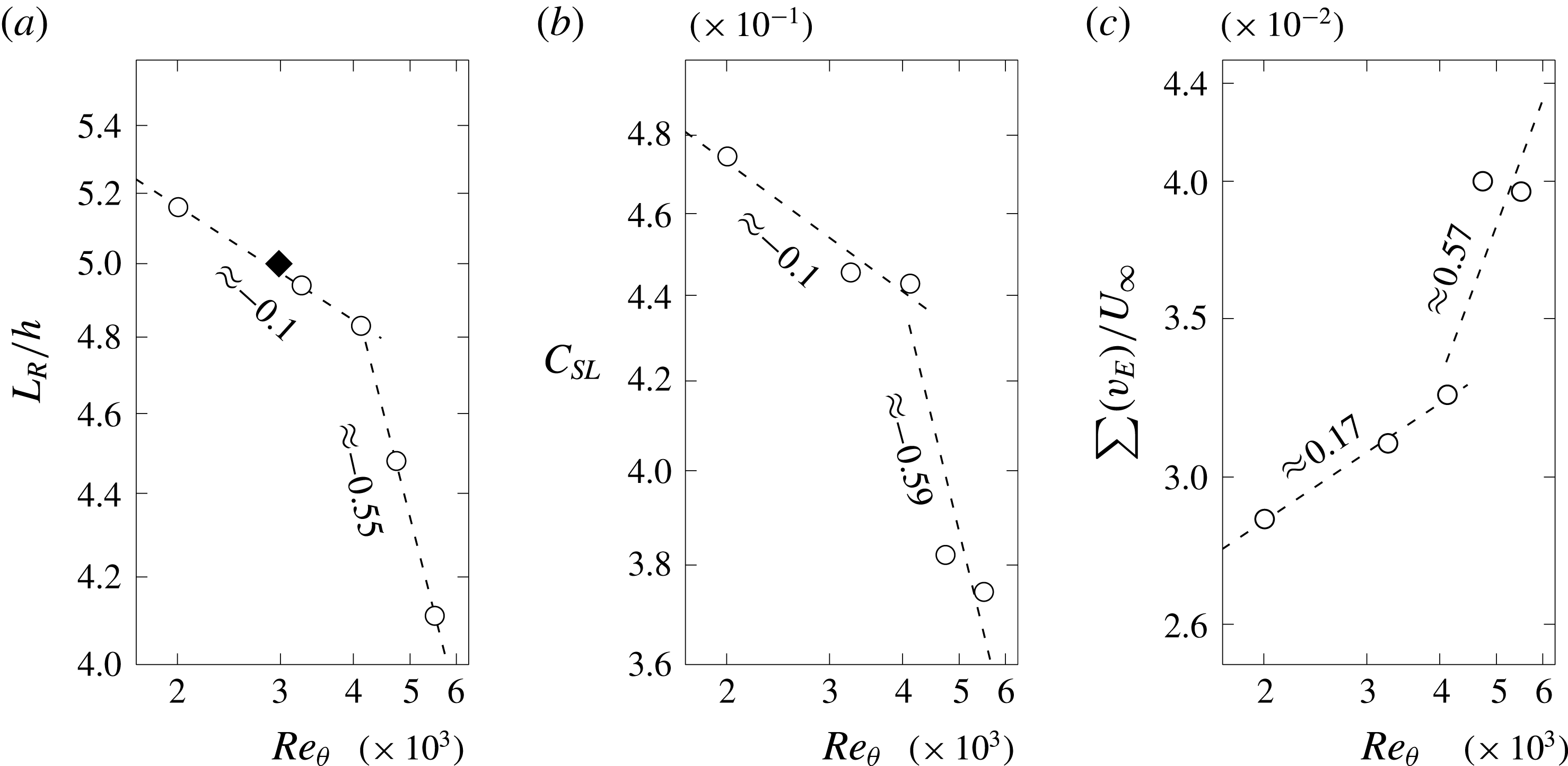
relates to shear layer development. It is found that
 $L_{R}/h$
evolves as
 $Re_{\unicode[STIX]{x1D703}}^{m}$
(shown in figure 11
a), where
 $m$
is a negative power, at least on the available range of
 $Re_{\unicode[STIX]{x1D703}}$
. This relationship seems to be robust to
 $\unicode[STIX]{x1D6FF}/h$
, since the point reported by Kourta et al. (Reference Kourta, Thacker and Joussot2015) (
 $Re_{\unicode[STIX]{x1D703}}=2983$
,
 $L_{R}/h=5$
) falls well within the trend defined by measurements taken in this study. Surprisingly, our measurements reveal that
 $m$
changes abruptly from
 $-0.1$
to
 $-0.55$
around a critical value
 $Re_{\unicode[STIX]{x1D703}c}=4100$
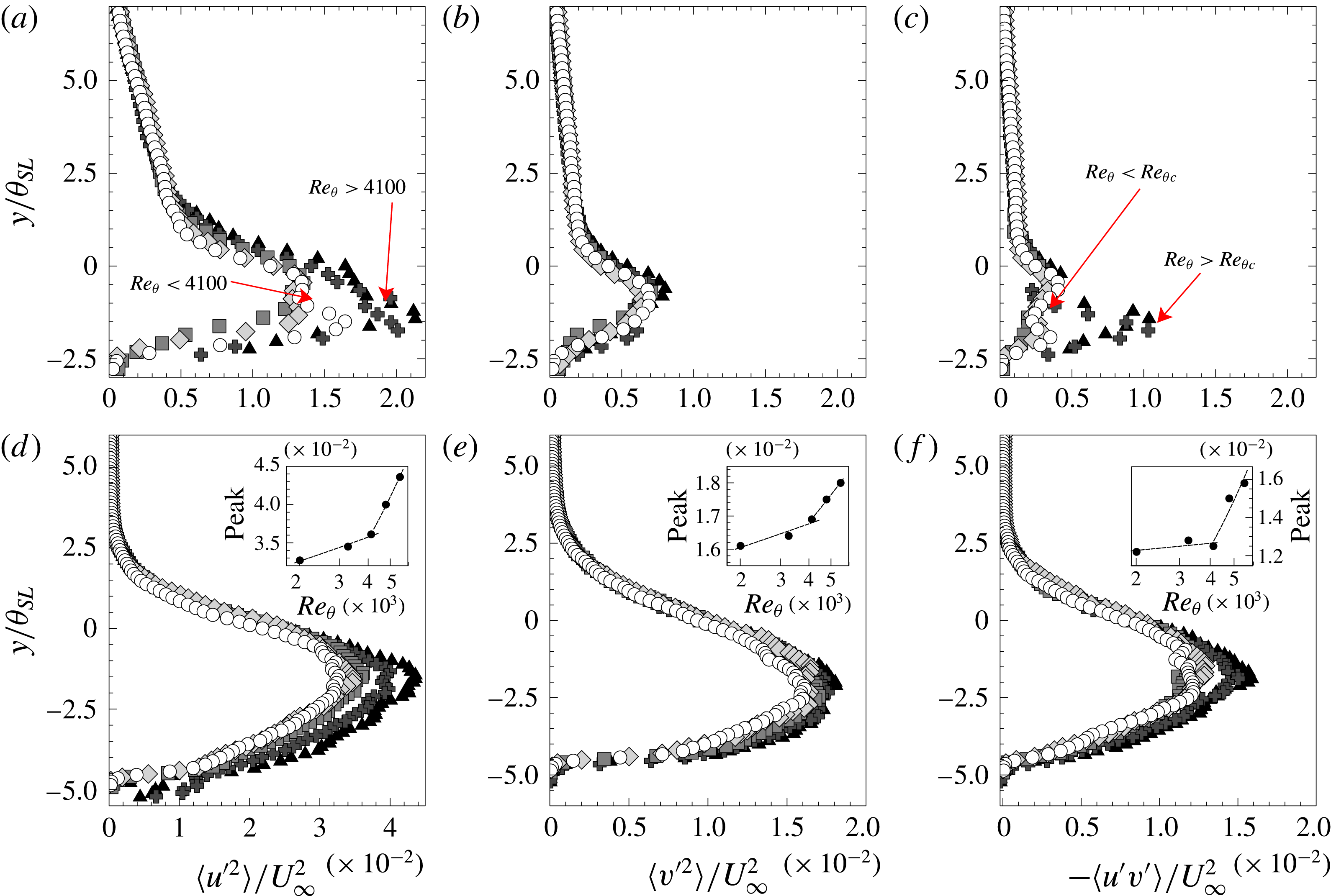
. This seems to be linked to the evolution of the turbulent state of the flow. Figure 12 presents the vertical profiles of Reynolds stresses at
 $x/L_{R}\approx 0.1$
and
 $x/L_{R}\approx 0.8$
for all available
 $Re$
. The curves are normalised on
 $\unicode[STIX]{x1D703}_{SL}$
and
 $U_{\infty }$
. Let us use
 $Re_{\unicode[STIX]{x1D703}c}$
to discriminate low
 $Re_{\unicode[STIX]{x1D703}}$
from high
 $Re_{\unicode[STIX]{x1D703}}$
. Figure 12(a–c) shows that at
 $x/L_{R}\approx 0.1$
Reynolds stresses scale relatively well with
 $\unicode[STIX]{x1D703}_{SL}$
and
 $U_{\infty }$
both at low and high
 $Re_{\unicode[STIX]{x1D703}}$
, separately. However, we observe that peak values of
 $\langle u^{\prime 2}\rangle$
and
 $-\langle u^{\prime }v^{\prime }\rangle$
for high and low
 $Re_{\unicode[STIX]{x1D703}}$
do not collapse, with much more intense turbulent levels at high
 $Re_{\unicode[STIX]{x1D703}}$
. This difference seems consistent with the change of power law found in figure 11. The turbulent level of the flow changes as one moves downstream of the mean separation point. Figure 12(d–f) highlights that, at
 $x/L_{R}\approx 0.8$
, Reynolds stress profiles are a more progressive function of
 $Re_{\unicode[STIX]{x1D703}}$
. Similar
 $Re_{\unicode[STIX]{x1D703}}$
dependencies of turbulent quantities have already been observed in separating/reattaching flows, for example by Song & Eaton (Reference Song and Eaton2003). However, peak values of Reynolds stresses also evolve as
 $Re_{\unicode[STIX]{x1D703}}^{m}$
, where
 $m$
is now positive. Once again
 $m$
changes abruptly around
 $Re_{\unicode[STIX]{x1D703}c}$
. The values of
 $m$
appear to change in the streamwise direction also, but the
 $Re_{\unicode[STIX]{x1D703}}$
trends shown in the inserts in figure 12(d–f) are representative. This further supports the interpretation suggested by figure 11, i.e. that
 $L_{R}$
decreases with increasing turbulence levels.
Log–log plot in function of
 $Re_{\unicode[STIX]{x1D703}}$
of (a)
 $L_{R}/h$
; (b) the parameter
 $C_{SL}=\langle -\unicode[STIX]{x1D703}_{SL}/(2hR_{uv}^{\ast })\rangle$
; (c)
 $(v_{E}^{A}|_{RRI}+v_{E}^{A}|_{TNTI})/U_{\infty }$
on
 $x/L_{R}\in (0,0.5)$
. Symbols: ○ present work; – – – Power-law fits (in the sense of least-mean square);
 $\blacklozenge$
Kourta et al. (Reference Kourta, Thacker and Joussot2015), data at
 $Re_{h}=2\times 10^{5}$
.

Reynold stresses
 $\langle u^{\prime 2}\rangle$
,
 $\langle v^{\prime 2}\rangle$
and
 $-\langle u^{\prime }v^{\prime }\rangle$
in the separated shear layer at (a–c)
 $x/L_{R}\approx$
0.1 and (d–f)
 $x/L_{R}\approx$
0.8. Inserts in (d–f) show the
 $Re_{\unicode[STIX]{x1D703}}^{m}$
evolution of the peak of
 $\langle u^{\prime 2}\rangle$
,
 $\langle v^{\prime 2}\rangle$
and
 $-\langle u^{\prime }v^{\prime }\rangle$
, respectively. At
 $x/L_{R}\approx$
0.8, the exponent
 $m$
passes from 0.05–0.1 to 0.65–0.80 (0.22 for
 $\langle v^{\prime 2}\rangle$
). Other symbols as in figure 6.

4.2 RANS equation in the separated shear layer
It seems now wise to give some physical underpinning to these observations. To begin with, let us consider the transport equation for mean momentum. Putting in evidence the pressure term, one can write:
 $$\begin{eqnarray}\frac{1}{\unicode[STIX]{x1D70C}}\frac{\unicode[STIX]{x2202}p}{\unicode[STIX]{x2202}x_{i}}=-U_{j}\frac{\unicode[STIX]{x2202}U_{i}}{\unicode[STIX]{x2202}x_{j}}+\unicode[STIX]{x1D708}\frac{\unicode[STIX]{x2202}^{2}U_{i}}{\unicode[STIX]{x2202}x_{j}^{2}}-\frac{\unicode[STIX]{x2202}}{\unicode[STIX]{x2202}x_{j}}\langle u_{i}^{\prime }u_{j}^{\prime }\rangle ,\end{eqnarray}$$
where repeated indexes indicate summation. PIV data give access to all quantities on the right-hand side of (4.1) (see appendix A). The results presented at § 3.3 prove that the development of the shear layer is correlated to the longitudinal pressure gradient. Then, we first focus on the mean streamwise momentum transport equation, which by dropping negligible terms is rewritten as:
 $$\begin{eqnarray}\frac{\unicode[STIX]{x2202}p}{\unicode[STIX]{x2202}x}\approx -\unicode[STIX]{x1D70C}\frac{\unicode[STIX]{x2202}}{\unicode[STIX]{x2202}y}\left(UV+\langle u^{\prime }v^{\prime }\rangle \right)-\unicode[STIX]{x1D70C}\frac{\unicode[STIX]{x2202}\langle u^{\prime 2}\rangle }{\unicode[STIX]{x2202}x}.\end{eqnarray}$$
The relative weight of the terms on the right-hand side of (4.2) evolves in the streamwise direction. In particular, figure 13(a) shows their evolution along the RRI. It appears that the convective term
 $V\unicode[STIX]{x2202}U/\unicode[STIX]{x2202}y$
, related to the main component of mean shear, is dominant in the neighbourhood of the separation point. This is no longer the case in the neighbourhood of the reattachment point (
 $x/L_{R}\approx 0.7$
), where
 $\unicode[STIX]{x2202}\langle u^{\prime }v^{\prime }\rangle /\unicode[STIX]{x2202}y$
dominates the other terms and causes
 $\unicode[STIX]{x2202}p/\unicode[STIX]{x2202}x$
to reach its maximum.
Longitudinal pressure gradient at
 $Re_{h}=5\times 10^{4}$
(a) along the RRI; (b) along the TNTI. Symbols: ○
 $\unicode[STIX]{x2202}\langle u^{\prime 2}\rangle /\unicode[STIX]{x2202}x$
;

 $\unicode[STIX]{x2202}\langle u^{\prime }v^{\prime }\rangle /\unicode[STIX]{x2202}y$
; ▴
 $\unicode[STIX]{x2202}UV/\unicode[STIX]{x2202}y$
;

 $\unicode[STIX]{x2202}\langle v^{\prime 2}\rangle /\unicode[STIX]{x2202}x$
; - - - - -
 $\unicode[STIX]{x2202}\langle u^{\prime }v^{\prime }\rangle /\unicode[STIX]{x2202}y+\unicode[STIX]{x2202}\langle u^{\prime 2}\rangle /\unicode[STIX]{x2202}x$
; —— (red online)
 $\unicode[STIX]{x2202}p/\unicode[STIX]{x2202}x$
, computed as in (4.1);

 $\unicode[STIX]{x2202}p/\unicode[STIX]{x2202}x$
at the TNTI, computed as in (4.6). All curves are normalised on dynamic pressure and step height
 $h$
.

We now investigate the RANS equation for the vertical velocity component
 $v$
. Neglecting smaller terms listed in appendix A, equation (4.1) becomes:
 $$\begin{eqnarray}\frac{\unicode[STIX]{x2202}p}{\unicode[STIX]{x2202}y}\approx -\unicode[STIX]{x1D70C}\frac{\unicode[STIX]{x2202}\langle v^{\prime 2}\rangle }{\unicode[STIX]{x2202}y}.\end{eqnarray}$$
It is observed that
 $\unicode[STIX]{x2202}p/\unicode[STIX]{x2202}y$
always favours an injection of mass into
 ${\mathcal{V}}_{c}$
, because here
 $\langle v^{\prime 2}\rangle$
is higher than inside the recirculation region or in the external flow (Cuvier Reference Cuvier2012; Kourta et al.
Reference Kourta, Thacker and Joussot2015). However, on most of the large field
 $\unicode[STIX]{x2202}p/\unicode[STIX]{x2202}y$
is not well correlated to local mass fluxes. Following Pope (Reference Pope2000), equation (4.3) can be integrated to:
 $$\begin{eqnarray}p/\unicode[STIX]{x1D70C}=p_{0}/\unicode[STIX]{x1D70C}-\langle v^{\prime 2}\rangle ,\end{eqnarray}$$
where
 $p_{0}$
is the pressure in the free flow. The streamwise pressure gradient can then be computed by taking the derivative of (4.4), which gives:
 $$\begin{eqnarray}\frac{1}{\unicode[STIX]{x1D70C}}\frac{\unicode[STIX]{x2202}p}{\unicode[STIX]{x2202}x}=\frac{1}{\unicode[STIX]{x1D70C}}\frac{\text{d}p_{0}}{\text{d}x}-\frac{\unicode[STIX]{x2202}\langle v^{\prime 2}\rangle }{\unicode[STIX]{x2202}x}.\end{eqnarray}$$
By plugging into (4.2), this yields for the mean RRI:
 $$\begin{eqnarray}\frac{\text{d}p_{0}}{\text{d}x}\approx -\unicode[STIX]{x1D70C}\left(\frac{\unicode[STIX]{x2202}}{\unicode[STIX]{x2202}y}\left(UV+\langle u^{\prime }v^{\prime }\rangle \right)+\frac{\unicode[STIX]{x2202}}{\unicode[STIX]{x2202}x}\left(\langle u^{\prime 2}\rangle -\langle v^{\prime 2}\rangle \right)\right).\end{eqnarray}$$
Now, if one considers that the mean TNTI bounds the free flow, equation (4.6) evaluated at the mean RRI should at least approximate the evolution of the pressure gradient along the TNTI. Figure 13(b) reports the longitudinal pressure gradient along the TNTI at
 $Re_{h}=5\times 10^{4}$
, computed with both (4.1) (evaluated at the TNTI) and (4.6) (evaluated at the RRI). Similar results are obtained at all
 $Re_{h}$
and are not shown for sake of simplicity. The agreement of the two curves is not completely satisfactory in the first part of the separated region, but tendencies are clearly the same throughout the flow. This should confirm, at least qualitatively, that the mean pressure distribution connects the two mean interfaces on scales of the order of
 $L_{R}$
.
4.3 On the role of turbulent shear stresses
The prominent role of
 $\unicode[STIX]{x2202}\langle u^{\prime }v^{\prime }\rangle /\unicode[STIX]{x2202}x$
at reattachment is consistent with important past results, that can be invoked to develop the present analysis. In particular, close to reattachment, Chapman et al. (Reference Chapman, Kuehn and Larson1958) wrote:
 $$\begin{eqnarray}\frac{\unicode[STIX]{x2202}p}{\unicode[STIX]{x2202}x}\approx -\unicode[STIX]{x1D70C}\frac{\unicode[STIX]{x2202}\langle u^{\prime }v^{\prime }\rangle }{\unicode[STIX]{x2202}y}.\end{eqnarray}$$
Figure 12 suggests that
 $\langle u^{\prime }v^{\prime }\rangle \sim R_{uv}^{\ast }U_{\infty }^{2}$
, where
 $R_{uv}^{\ast }$
is a local turbulent shear-stress intensity, and that
 $\unicode[STIX]{x2202}/\unicode[STIX]{x2202}y\sim 1/\unicode[STIX]{x1D703}_{SL}$
within the shear layer. It is pointed out that for similar considerations Chapman et al. (Reference Chapman, Kuehn and Larson1958) suggested to scale the
 $y$
axis with a displacement thickness
 $\unicode[STIX]{x1D6FF}^{\ast }$
. The two scalings are equivalent, at least for dimensional analysis. Normalising all terms of (4.7) gives:
 $$\begin{eqnarray}\frac{\unicode[STIX]{x2202}C_{p}}{\unicode[STIX]{x2202}x^{\ast }}\frac{1/2\unicode[STIX]{x1D70C}U_{\infty }^{2}}{X}\approx -\unicode[STIX]{x1D70C}\frac{\unicode[STIX]{x2202}\langle u^{\prime }v^{\prime }\rangle ^{\ast }}{\unicode[STIX]{x2202}y^{\ast }}\frac{R_{uv}^{\ast }U_{\infty }^{2}}{\unicode[STIX]{x1D703}_{SL}},\end{eqnarray}$$
where the superscript
 $^{\ast }$
indicates normalisation and
 $X$
is a characteristic streamwise scale. On dimensional grounds, equation (4.8) is a valid approximation of the RANS equation if:
 $$\begin{eqnarray}X\sim -\frac{\unicode[STIX]{x1D703}_{SL,r}}{2R_{uv,r}^{\ast }}\approx \frac{0.2h}{0.026}\approx 7.7h\sim L_{R},\end{eqnarray}$$
where the empirical values of
 $\unicode[STIX]{x1D703}_{SL,r}$
and
 $R_{uv,r}^{\ast }$
were calculated at the mean reattachment point. Equation (4.9) shows that
 $L_{R}$
depends on the interaction of the separated shear layer with the wall. Also, the agreement between the numerical value of
 $X$
(7.7
 $h$
) and the position of
 $C_{p,r}$
(
 ${\approx}7h$
) is impressive, if one considers the relative simplicity of the premises to (4.7). This confirms the idea that the pressure rise is one of the main effects of the interaction of the separated shear layer with the wall, at least for the present value of
 $ER$
. In the framework of this section, however, the most important suggestion given by (4.9) is that
 $L_{R}$
should be a function of shear layer properties in a neighbourhood of reattachment. Hence, taking into account that
 $h$
is constant in this study, one should verify that at least in the mean:
 $$\begin{eqnarray}C_{SL}=-\overline{\frac{\unicode[STIX]{x1D703}_{SL}}{2hR_{uv}^{\ast }}}\sim L_{R}/h\sim \left\{\begin{array}{@{}ll@{}}Re_{\unicode[STIX]{x1D703}}^{-0.1},\quad & \text{if }Re_{\unicode[STIX]{x1D703}}<Re_{\unicode[STIX]{x1D703}c},\\ Re_{\unicode[STIX]{x1D703}}^{-0.55},\quad & \text{if }Re_{\unicode[STIX]{x1D703}}>Re_{\unicode[STIX]{x1D703}c}.\end{array}\right.\end{eqnarray}$$
In (4.10), the overline symbol indicates the average over a streamwise domain within
 $L_{R}$
where (4.7) is valid, i.e.
 $x/L_{R}\in \left[0.7,1\right]$
. The
 $Re_{\unicode[STIX]{x1D703}}$
trend of
 $C_{SL}$
is shown in figure 11(b). Very good agreement with figure 11(a) is obtained both at low and high
 $Re_{\unicode[STIX]{x1D703}}$
. We stress the importance of this latter result, that provides new insight in the functioning and possible control of separating/reattaching shear layers, as follows. The size of the recirculation region relative to step height (and more in general those features of the flow that scale with it) is strongly influenced by the interactions of the shear layer with the wall. The latter depend on the turbulent properties of the shear layer in the neighbourhood of reattachment, which are in turn correlated to the turbulent state of the incoming boundary layer, represented by
 $Re_{\unicode[STIX]{x1D703}}$
. Since the pressure rise at reattachment seems to be one of the consequences of impingement, in the mean the fluidic system composed by the incoming boundary layer, the separated shear layer and the wall might behave like a closed loop, in which the (favourable) pressure gradient induced upstream of separation acts as a feedback branch, influencing properties of the incoming boundary layer. This might explain why boundary layer quantities (e.g.
 $\unicode[STIX]{x1D6FF}/h$
and
 $Re_{\unicode[STIX]{x1D703}}$
) estimated far upstream of separation show some degree of correlation with properties of the separated shear layer (see Neumann & Wengle Reference Neumann and Wengle2003 and § 2.2.1). Also, it appears that controlling turbulent shear-stress intensity within the shear layer or possibly within the incoming boundary layer could be an efficient strategy to reduce
 $L_{R}$
and eventually reattach the shear layer to the ramp.
Further work is needed to better assess the validity of both correlations presented in figure 11(a,b). In particular, more precise data are required to understand the local behaviour of the exponent
 $m$
: the good collapse with
 $h$
shown by
 $\unicode[STIX]{x1D703}_{SL}$
(figure 6) suggests that
 $\langle R_{uv}^{\ast }\rangle \sim 1/L_{R}$
, but in principle the relationship between
 $\unicode[STIX]{x1D703}_{SL}$
and
 $R_{uv}^{\ast }$
might itself be a function of
 $Re_{\unicode[STIX]{x1D703}}$
. In spite of these open questions,
 $\unicode[STIX]{x1D703}$
and
 $L_{R}$
will be used as scaling parameters in the following sections.
4.4 On the role of mean shear
Thanks to available PIV data, the approach of Chapman et al. (Reference Chapman, Kuehn and Larson1958) can be extended to the investigation of a neighbourhood of the separation point with very little effort. Figure 13 shows that the convective term
 $\unicode[STIX]{x2202}UV/\unicode[STIX]{x2202}y$
determines the pressure gradient in this region, since Reynolds stresses balance each other. Then, equation (4.2) can be rewritten as:
 $$\begin{eqnarray}\frac{\unicode[STIX]{x2202}p}{\unicode[STIX]{x2202}x}\approx -\unicode[STIX]{x1D70C}\frac{\unicode[STIX]{x2202}UV}{\unicode[STIX]{x2202}y}.\end{eqnarray}$$
Of course, one can put
 $U\sim U_{\infty }$
. Since the mean flow is almost bidimensional (see § 3.3), by applying the continuity equation to the recirculation region one obtains
 $V\sim U_{\infty }Y/L_{R}$
, where
 $Y$
is a suitable vertical scale of the recirculation region. Then, normalising (4.11) gives:
 $$\begin{eqnarray}\frac{\unicode[STIX]{x2202}C_{p}}{\unicode[STIX]{x2202}x^{\ast }}\frac{1/2\unicode[STIX]{x1D70C}U_{\infty }^{2}}{X}\approx -\unicode[STIX]{x1D70C}\frac{\unicode[STIX]{x2202}U^{\ast }V^{\ast }}{\unicode[STIX]{x2202}y^{\ast }}\frac{U_{\infty }^{2}Y}{YL_{R}},\end{eqnarray}$$
where the same notation as in (4.7) applies. Dimensional analysis then yields:
 $$\begin{eqnarray}X\sim \frac{L_{R}}{2}.\end{eqnarray}$$
If it is accepted that (4.11) represents at least the dominant feature of a free shear layer, equation (4.13) states that in presence of a wall a free shear layer approximation holds just up to
 $x/L_{R}\approx 0.5$
. This is pleasingly consistent with the considerations of § 3.2. However, it must be stressed that the growth rate of the shear layer is influenced by the interaction with the wall even for
 $x/L_{R}<0.5$
: since
 $L_{R}/h\sim \left(\text{d}\unicode[STIX]{x1D703}_{SL}/\text{d}x\right)^{-1}$
(§ 3.2), it follows immediately that
 $\left(\text{d}\unicode[STIX]{x1D703}_{SL}/\text{d}x\right)\sim C_{SL}^{-1}$
. The presence of the wall might then explain why measured growth rates do not match free shear layer models perfectly.
5 TNTI detection
The TNTI and the RRI have a central role in this work because they provide a set of boundaries at which to study mean entrainment. In addition, their multiscale nature (see figure 1) allows an attempt to extend the investigation beyond the analysis of the mean field of the previous section, to the role of turbulent scales. The definition of mean RRI was already introduced at § 3.2 and its possible extension to instantaneous fields is straightforward. The present section will then detail how the TNTI is detected on the instantaneous and mean velocity fields.
This study follows the TNTI detection method developed by de Silva et al. (Reference de Silva, Philip, Chauhan, Meneveau and Marusic2013) and Chauhan et al. (Reference Chauhan, Philip, de Silva, Hutchins and Marusic2014), which exclusively relies on PIV images to detect the TNTI of an equilibrated turbulent boundary layer. The method will be recalled here briefly, as it is explained in detail in their original papers. The PIV velocity fields are used to compute
 $\tilde{k}$
, a dimensionless, turbulent kinetic energy locally averaged on a square kernel.
 $\tilde{k}$
is close to zero in the irrotational field, but it increases rapidly in the turbulent one. Then, a threshold value
 $\tilde{k}_{th}$
identifying the instantaneous TNTI can be computed iteratively. The retained
 $\tilde{k}_{th}$
is the one for which the following criterion is fulfilled:
 $$\begin{eqnarray}Z_{i}+3\unicode[STIX]{x1D70E}_{i}\approx \unicode[STIX]{x1D6FF},\end{eqnarray}$$
where
 $Z_{i}$
and
 $\unicode[STIX]{x1D70E}_{i}$
are respectively the mean and the standard deviation of the position of the TNTI above the wall. This method is attractive because it can be applied with virtually no extra experimental cost compared to usual PIV measurements, and with reasonable extra post-processing. In addition, the definition of
 $\tilde{k}$
can be easily modified to better take into account the contribution to turbulent energy of the vertical velocity component over the separation. We then define
 $\tilde{k}$
in percentage of mean free-stream energy, as:
 $$\begin{eqnarray}\tilde{k}=\frac{100}{9(U_{\infty }^{2}+V_{\infty }^{2})}\mathop{\sum }_{m,n=-1}^{1}[(u_{m,n}-U_{\infty })^{2}+(v_{m,n}-V_{\infty })^{2}],\end{eqnarray}$$
where
 $U_{\infty }$
and
 $V_{\infty }$
are respectively the streamwise and the wall-normal components of the local, free-stream velocity. In (5.2) the side of the kernel is equal to 3 correlation windows and the indexes
 $m$
and
 $n$
allow us to iterate on the two dimensions of the kernel. For the sake of clarity, the dependencies on
 $(x)$
of
 $U_{\infty }$
and
 $V_{\infty }$
and on
 $(x,y)$
of
 $u_{m,n}$
and
 $v_{m,n}$
were omitted. Since the original convergence criterion given by (5.1) cannot be directly applied to the massive separation,
 $\tilde{k}_{th}$
is computed on the boundary layer images provided by the auxiliary field. Then,
 $\tilde{k}_{th}$
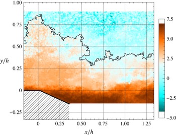
is applied to the other PIV fields, to detect the TNTI above the massive separation. Figure 14 shows one instantaneous TNTI over the detailed field. Results over the large field are comparable, but at a lower resolution. Following Chauhan et al. (Reference Chauhan, Philip, de Silva, Hutchins and Marusic2014), pockets of inhomogeneous fluid that are found on both sides of the TNTI were filtered out.
Although the choice of
 $\tilde{k}_{th}$
was data driven and consistent with experimental conditions (in particular
 $Re_{h}$
), no particular trend is found with respect to
 $Re_{h}$
. Table 3 shows that in most cases one can put
 $\tilde{k}_{th}\approx 0.35$
. Scatter of threshold values, in particular at
 $Re_{h}=4\times 10^{4}$
, appears to be due to slightly different levels of PIV noise and to the quality of the PIV fields in general. However statistics of TNTI position presented in table 4 seem much less sensitive to these issues, suggesting that noise mostly affects the value of
 $\tilde{k}_{th}$
, rather than the position of the detected TNTI. PIV resolution has a sizeable effect on the value of
 $\tilde{k}_{th}$
(
 $-30$
% if the size of the PIV correlation window is increased from
 $16\times 16~\text{px}^{2}$
to
 $48\times 48~\text{px}^{2}$
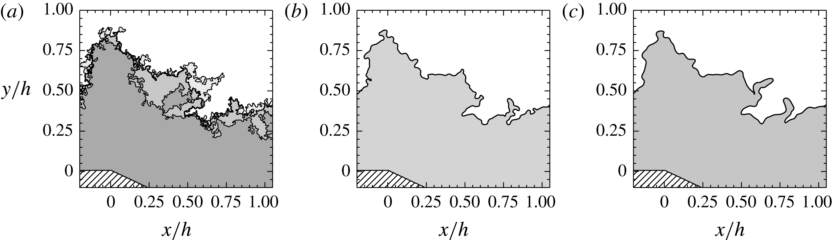
) but instantaneous TNTIs prove to be qualitatively robust to resolution and more in general to the choice of
 $\tilde{k}_{th}$
(see figure 15). This supports the choice of also applying the values of
 $\tilde{k}_{th}$
computed on the auxiliary field to the finer images of the detailed field, and allows comparison between the latter and the large field.
Instantaneous TNTI detected over the detailed field at
 $Re_{h}=5\times 10^{4}$
. The colormap represents the distribution of
 $\ln \tilde{k}$
.

Instantaneous TNTI detected on the detailed field at
 $Re_{h}=5\times 10^{4}$
, at different spatial resolutions. (a)
 $\unicode[STIX]{x1D6E5}/h=6.4\times 10^{-3}$
. The grey scale highlights the evolution of the detected turbulent region if the threshold value is tuned within
 $\tilde{k}_{th}\pm 50\,\%$
. Darker shades of grey are used for higher threshold values; (b)
 $\unicode[STIX]{x1D6E5}/h=1.3\times 10^{-2}$
; (c)
 $\unicode[STIX]{x1D6E5}/h=1.9\times 10^{-2}$
.

TNTI detection was assessed based on several a posteriori observations. Firstly, converged
 $Z_{i}$
and
 $\unicode[STIX]{x1D70E}_{i}$
are comparable to those in the literature (see table 4 and references in Chauhan et al. (Reference Chauhan, Philip, de Silva, Hutchins and Marusic2014)). Secondly,
 $\tilde{k}_{th}$
values are of the same order of magnitude as those reported by de Silva et al. (Reference de Silva, Philip, Chauhan, Meneveau and Marusic2013) and Chauhan et al. (Reference Chauhan, Philip, de Silva, Hutchins and Marusic2014). Even though exact quantitative comparison with such different experiments seems inappropriate, this element is reassuring if one keeps in mind that the wind tunnel at Prisme Laboratory and the facility used in those studies have comparable levels of free-stream turbulence and PIV noise. Finally, TNTI robustness to detection thresholds ensures that, to some extent, uncertainties on
 $\tilde{k}_{th}$
will not impact our conclusions significantly.
Value of
 $\tilde{k}_{th}$
at different
 $Re_{h}$
.

Comparison of mean value and standard deviation of TNTI position in the boundary layer. Other references are reported in Chauhan et al. (Reference Chauhan, Philip, de Silva, Hutchins and Marusic2014).

Once a suitable
 $\tilde{k}_{th}$
has been chosen, the mean TNTI (shown in figure 5) can be computed either by detecting the
 $\tilde{k}_{th}$
isoline on the mean
 $\tilde{k}$
field or as the set of points where intermittency
 $\unicode[STIX]{x1D6FE}$
is equal to 0.5 (Corrsin & Kistler Reference Corrsin and Kistler1955). Alternatively, Maurice et al. (Reference Maurice, Thiesset, Halter, Mazellier, Chauveau, Gökalp and Kourta2016) showed that the mean position of a turbulent interface (viz. a flame) is also obtained by averaging the positions of a large set of its instantaneous realisations. As a side note, it is pointed out that the energy-based definition of the TNTI is not consistent with the velocity-based definition of the RRI. The work of Kwon et al. (Reference Kwon, Philip, Silva, Hutchins and Monty2014) suggests that the TNTI could also be detected with a velocity criterion, with very good agreement with the approach used here. However, since this inconsistency does not impact the computation of mass fluxes, it is more convenient to adopt the energy-based definition of the TNTI. This choice allows a simple use of (7.4), on which a large part of § 7 is developed.
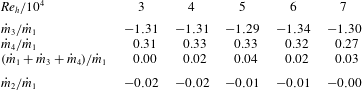
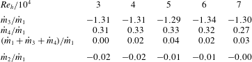
Mass fluxes normalised on
 ${\dot{m}}_{1}$
, the mass flux due to the incoming boundary layer.
6 Mean field mass entrainment
This section investigates mass entrainment in the mean field, by quantifying the mass fluxes exchanged through both the mean TNTI and the mean RRI. Since the mean field is bidimensional (see figure 8), the use of mass fluxes computed from PIV images is justified.
6.1 Mean mass balance
To begin with, a mean mass balance is computed over the fixed control volume
 ${\mathcal{V}}_{c}$
shown in figure 5.
 ${\mathcal{V}}_{c}$
is delimited by the mean TNTI, the mean RRI and two vertical sections, placed at the position of the mean separation and reattachment points. Note that the volume
 ${\mathcal{V}}_{c}$
encompasses the mean separated shear layer. The total mass flux per spanwise unit length through one boundary of
 ${\mathcal{V}}_{c}$
is given by:
 $$\begin{eqnarray}{\dot{m}}_{i}=-\unicode[STIX]{x1D70C}\int _{L_{i}}\boldsymbol{U}(l)\boldsymbol{\cdot }\boldsymbol{n}(l)\,\text{d}l=-\unicode[STIX]{x1D70C}\int _{L_{i}}(U(l)\sin (\unicode[STIX]{x1D719}(l))+V(l)\cos (\unicode[STIX]{x1D719}(l)))\,\text{d}l,\end{eqnarray}$$
where
 $\unicode[STIX]{x1D70C}$
is air density,
 $L_{i}$
is the length of one boundary,
 $l$
a curvilinear abscissa,
 $\boldsymbol{n}(l)$
is the local normal to the boundary (pointing outward of
 ${\mathcal{V}}_{c}$
) and
 $\unicode[STIX]{x1D719}$
is the angle between
 $\boldsymbol{n}(l)$
and the
 $Y$
axis. Due to the different definitions of the two interfaces, it is
 $\boldsymbol{n}(l)_{TNTI}=-\unicode[STIX]{x1D735}\tilde{k}/|\unicode[STIX]{x1D735}\tilde{k}|$
and
 $\boldsymbol{n}(l)_{RRI}=-\unicode[STIX]{x1D735}U/|\unicode[STIX]{x1D735}U|$
. It is worth noticing that
 ${\dot{m}}_{2}$
must be zero, since the RRI is the only permeable boundary of the recirculation bubble, which is, on average, two-dimensional and stationary. This is consistent with the idea that backflow and shear layer entrainment through the RRI must balance out (Chapman et al.
Reference Chapman, Kuehn and Larson1958; Adams & Johnston Reference Adams and Johnston1988b
). The topology of the flow also suggests that
 ${\dot{m}}_{1}$
(at the mean separation point) will be positive and
 ${\dot{m}}_{3}$
(at the mean reattachment point) negative. Since in general the TNTI is not a streamline, it will be
 ${\dot{m}}_{4}={\dot{m}}_{3}-{\dot{m}}_{1}\neq 0$
. The scaling of
 ${\dot{m}}_{4}$
can be predicted on dimensional grounds. With good approximation, the right-hand side of (1.1) can be rewritten as:
 $$\begin{eqnarray}\unicode[STIX]{x1D70C}v_{E}^{A}L^{A}\approx {\dot{m}}_{4}.\end{eqnarray}$$
It is straightforward to see from figure 5 that the length of the mean TNTI above the recirculation region scales with
 $L_{R}$
. Following § 4.1, it is then
 $L^{A}\sim L_{R}\sim h\,Re_{\unicode[STIX]{x1D703}}^{m}$
. Since
 $\unicode[STIX]{x1D719}$
is small along both the mean RRI and the mean TNTI, from (6.1)
 $v_{E}^{A}$
could be approximated as follows:
 $$\begin{eqnarray}v_{E}^{A}\sim U_{\infty }\unicode[STIX]{x1D719}_{TNTI}+V.\end{eqnarray}$$
The geometry of the problem suggests that
 $\unicode[STIX]{x1D719}\sim h/L_{R}$
, at least for the present values of
 $h$
and
 $L_{R}$
. This comes to say that the slope of the TNTI relates to shear layer development, as in the case of the RRI (§ 3.2). The continuity equation can be invoked to obtain the scaling of
 $V$
(see § 4.4). We put
 $Y=h$
, so that
 $V\sim U_{\infty }h/L_{R}$
. This relationship can be interpreted as a measure of streamline deviation due to the ramp: the steeper is the deviation, the higher will be the vertical velocity component acquired by the flow. Finally, it is
 $v_{E}^{A}\sim U_{\infty }h/L_{R}$
, which implies that:
 $$\begin{eqnarray}{\dot{m}}_{4}\sim \unicode[STIX]{x1D70C}U_{\infty }Re_{\unicode[STIX]{x1D703}}^{-m}hRe_{\unicode[STIX]{x1D703}}^{m}\sim \unicode[STIX]{x1D70C}U_{\infty }h.\end{eqnarray}$$
Minding that
 $h$
is constant in this study,
 ${\dot{m}}_{4}$
should then scale with
 $U_{\infty }$
. Measured mean mass fluxes are reported in table 5. Uncertainties on the mass balance appear to be mainly due to laser reflections introducing corrupted velocity vectors near the wall. In any case, our results evidence that mass is not conserved within
 ${\mathcal{V}}_{c}$
: the TNTI contributes to the mass balance with at least 30 % of the mass injected into
 ${\mathcal{V}}_{c}$
by the separating boundary layer, which is by far not negligible. This confirms that entrainment of irrotational fluid plays an important role in the functioning of the separated shear layer. Equation (6.4) is also verified relatively well. Considering that
 ${\dot{m}}_{1}\sim U_{\infty }\unicode[STIX]{x1D6FF}$
and that
 $\unicode[STIX]{x1D6FF}\approx h$
in this study, it is possible to write:
 $$\begin{eqnarray}{\dot{m}}_{4}\approx 0.3\pm 0.03{\dot{m}}_{1}\approx 0.3\unicode[STIX]{x1D70C}U_{\infty }h,\end{eqnarray}$$
which is consistent with the prediction provided by (6.4). Taking into account all dependencies, this can be interpreted geometrically as follows: while the mean slope of the TNTI increases with
 $Re_{\unicode[STIX]{x1D703}}$
, the reduction (as
 $L_{R}$
) of mean TNTI length is compensated for by the higher contribution of velocity (due to increased streamline deviation).
6.2 Local mean mass fluxes
To gather information of a finer grain, let us now consider the normalised local mean fluxes per unit surface through the mean RRI and the mean TNTI. This extends the 0-dimensional analysis of § 6.1 by including the streamwise evolution of local mass fluxes. According to (6.1), the normalised local flux at each point of any of the two boundaries can be computed as:
 $$\begin{eqnarray}{\dot{m}}_{xi}^{\ast }=\frac{1}{\unicode[STIX]{x1D70C}U_{\infty }}\frac{\text{d}{\dot{m}}_{i}}{\text{d}l}=-\frac{1}{U_{\infty }}(U(l)\sin (\unicode[STIX]{x1D719}(l))+V(l)\cos (\unicode[STIX]{x1D719}(l))).\end{eqnarray}$$
6.2.1 Local mean fluxes through the RRI
The streamwise evolution of
 ${\dot{m}}_{x2}^{\ast }$
is reported in figure 16(a). It appears that all curves collapse nicely under a longitudinal scaling based on
 $L_{R}$
, which is consistent with findings of the previous sections.
 ${\dot{m}}_{x2}^{\ast }$
is very well correlated with local pressure gradients shown in figure 13(a). In addition,
 ${\dot{m}}_{x2}^{\ast }$
has an odd shape, with a sign inversion at
 $x/L_{R}\approx 0.5$
and almost antisymmetrical peaks, which is compatible with the mean mass flux through the RRI being zero (see § 6.1). On this basis, the analysis of
 ${\dot{m}}_{x2}^{\ast }$
for, say,
 $x/L_{R}<0.5$
can provide information on the scaling of fluxes through the entire RRI, even if
 ${\dot{m}}_{2}=0$
. Considering the scaling of figure 16(a), the integral of
 ${\dot{m}}_{x2}^{\ast }/L_{R}$
over
 $x/L_{R}<0.5$
will give:
 $$\begin{eqnarray}\frac{1}{\unicode[STIX]{x1D70C}U_{\infty }L_{R}}\int _{0}^{L_{R}/2}\frac{\text{d}{\dot{m}}_{i}}{\text{d}l}\text{d}l=\frac{1}{U_{\infty }L_{R}}\int _{0}^{L_{R}/2}\boldsymbol{U}(l)\boldsymbol{\cdot }\boldsymbol{n}(l)\,\text{d}l\approx \frac{v_{E}^{A}}{U_{\infty }},\end{eqnarray}$$
where in analogy with (1.1)
 $v_{E}^{A}$
is the mean, large-scale entrainment velocity at the RRI. Based on data from the large PIV field, equation (6.7) gives
 $v_{E}^{A}/U_{\infty }\approx 0.0237\pm 0.002$
on the available
 $Re_{\unicode[STIX]{x1D703}}$
range. If this is so, the mean mass flux that goes through the recirculation region can be computed as:
 $$\begin{eqnarray}{\dot{m}}_{2}^{IN}=-{\dot{m}}_{2}^{OUT}\approx \unicode[STIX]{x1D70C}v_{E}^{A}L_{R}/2\sim \unicode[STIX]{x1D70C}U_{\infty }\,hRe_{\unicode[STIX]{x1D703}}^{m}.\end{eqnarray}$$
Generally speaking, the interpretation of (6.8) is not straightforward, since
 $\unicode[STIX]{x1D703}=\unicode[STIX]{x1D703}(U_{\infty })$
. However, it can be shown from table 1 that
 $\unicode[STIX]{x1D703}$
does not change much on the tested range of
 $U_{\infty }$
. Then, equation (6.8) can be approximated with:
 $$\begin{eqnarray}{\dot{m}}_{2}^{IN}=-{\dot{m}}_{2}^{OUT}\sim \unicode[STIX]{x1D70C}hU_{\infty }^{1+m}\sim \unicode[STIX]{x1D70C}h\left\{\begin{array}{@{}ll@{}}U_{\infty }^{0.9},\quad & \text{if }Re_{\unicode[STIX]{x1D703}}<Re_{\unicode[STIX]{x1D703}c},\\ U_{\infty }^{0.45},\quad & \text{if }Re_{\unicode[STIX]{x1D703}}>Re_{\unicode[STIX]{x1D703}c}.\end{array}\right.\end{eqnarray}$$
Figure 17 shows that this is well supported by the data for both low and high
 $Re_{\unicode[STIX]{x1D703}}$
. All in all, the amount of mass crossing (twice) the RRI appears to increase with
 $U_{\infty }$
, at least on the spanned
 $U_{\infty }$
range, in spite of the shrinking recirculation region. Such behaviour is remarkably different from the one observed at the TNTI and modelled by (6.4). In any case, if it is admitted that (1.1) might hold for a variety of turbulent interfaces, it is clear that (6.8) would provide the scaling of mean large-scale mass transfer
 $v_{E}^{A}L^{A}$
for the RRI.
Normalised local mass fluxes along (a) the RRI; (b) the TNTI. Symbols as in figure 6.

Evolution with
 $U_{\infty }$
of
 ${\dot{m}}_{2}^{IN}$
, the total mean flux going through the recirculation region.

Best fit exponents for the relation
 $v_{E}^{A}|_{TNTI}/U_{\infty }=Re_{\unicode[STIX]{x1D703}}^{q}$
(6.4), tested on the entire
 $L_{R}$
and on two domains within it. The expected value
 $-m$
is also given.
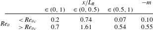
6.2.2 Local mean fluxes through the TNTI
Figure 16(b) presents the streamwise evolution of
 ${\dot{m}}_{x4}^{\ast }$
, which once again is very well correlated to the local pressure gradient (figure 13
b). An inflection is evident at
 $x/L_{R}\approx 0.5$
and a maximum is reached in the neighbourhood of the reattachment point. The scaling based on
 $U_{\infty }$
and
 $L_{R}$
is applied as in the case of the RRI, but a dependency on
 $Re_{\unicode[STIX]{x1D703}}$
is evident, which reminds the one observed in figure 12(a,c). This is not too surprising because, unlike along the RRI, equation (6.4) predicts that
 $v_{E}^{A}/U_{\infty }\sim Re_{\unicode[STIX]{x1D703}}^{-m}$
along the TNTI. It is interesting to use local mass fluxes through the TNTI to verify this latter relationship. Applying (6.7) to the TNTI over
 $x/L_{R}\in \left(0,1\right)$
and fitting a power law to its output yields
 $v_{E}^{A}/U_{\infty }\sim Re_{\unicode[STIX]{x1D703}}^{0.2}$
if
 $Re_{\unicode[STIX]{x1D703}}<Re_{\unicode[STIX]{x1D703}c}$
, and
 $v_{E}^{A}/U_{\infty }\sim Re_{\unicode[STIX]{x1D703}}^{0.7}$
if
 $Re_{\unicode[STIX]{x1D703}}>Re_{\unicode[STIX]{x1D703}c}$
. Although the change in slope at
 $Re_{\unicode[STIX]{x1D703}c}$
is well captured, the accuracy of this result is not completely satisfactory. The hint to a possible explanation is given by figure 16(b), which suggests that the intensity of transfer is not homogeneous along the TNTI. In particular, a simple integration along the TNTI allows us to verify that 80 %–90 % of
 ${\dot{m}}_{4}$
, slightly decreasing with
 $Re_{\unicode[STIX]{x1D703}}$
, is accounted for by the portion of the TNTI over
 $x/L_{R}\in \left(0.5,1\right)$
. Let us then separately test (6.4) on two distinct subregions of the TNTI, defined by the domains
 $x/L_{R}\in (0,0.5)$
and
 $x/L_{R}\in \left(0.5,1\right)$
. On each domain, values of
 $v_{E}^{A}/U_{\infty }$
are obtained with (6.7) and then fitted with power laws in the form
 $Re_{\unicode[STIX]{x1D703}}^{q}$
. Values of best fit exponents are reported in table 6. It appears clear that
 $v_{E}^{A}/U_{\infty }$
scales as predicted by (6.4) on
 $x/L_{R}\in \left(0.5,1\right)$
only, while faster power laws are observed on
 $x/L_{R}\in (0,0.5)$
. The extension of (6.4) to the whole TNTI is still a quite satisfactory approximation, as shown in § 6.1, because the second half of the TNTI contributes for most of transferred mass. As for
 $x/L_{R}\in (0,0.5)$
, its scaling seems to be determined by the free shear layer behaviour observed in this region, which in particular imposes
 $\text{d}\unicode[STIX]{x1D703}_{SL}/\text{d}x\sim Re_{\unicode[STIX]{x1D703}}^{-m}$
. Developing from Pope (Reference Pope2000) equation (5.222), one can put:
 $$\begin{eqnarray}\frac{\text{d}\unicode[STIX]{x1D703}_{SL}}{\text{d}x}\sim \frac{v_{E}^{A}|_{RRI}+v_{E}^{A}|_{TNTI}}{U_{\infty }}\sim Re_{\unicode[STIX]{x1D703}}^{-m}.\end{eqnarray}$$
This relationship is verified acceptably well with available data, in particular at high
 $Re_{\unicode[STIX]{x1D703}}$
(figure 11
c). The RRI contribution is found to be predominant, as it accounts for up to 80 % of
 $\text{d}\unicode[STIX]{x1D703}_{SL}/\text{d}x$
for
 $Re_{\unicode[STIX]{x1D703}}<Re_{\unicode[STIX]{x1D703}c}$
and up to 60 % for
 $Re_{\unicode[STIX]{x1D703}}>Re_{\unicode[STIX]{x1D703}c}$
. This being so, the evolution of
 $v_{E}^{A}|_{TNTI}/U_{\infty }$
must be faster than
 $Re_{\unicode[STIX]{x1D703}}^{-m}$
for (6.10) to be verified. With a known scaling law for
 $v_{E}^{A}|_{TNTI}/U_{\infty }$
, it is also possible to sketch the evolution of the mean amount of entrained mass on
 $x/L_{R}\in (0,0.5)$
. Since the length of the mean TNTI scales as
 $L_{R}$
, it will be:
 $$\begin{eqnarray}v_{E}^{A}L^{A}\sim U_{\infty }hRe_{\unicode[STIX]{x1D703}}^{q+m}=U_{\infty }h\left\{\begin{array}{@{}ll@{}}Re_{\unicode[STIX]{x1D703}}^{0.64},\quad & \text{if }Re_{\unicode[STIX]{x1D703}}<Re_{\unicode[STIX]{x1D703}c},\\ Re_{\unicode[STIX]{x1D703}}^{1.06},\quad & \text{if }Re_{\unicode[STIX]{x1D703}}>Re_{\unicode[STIX]{x1D703}c}.\end{array}\right.\end{eqnarray}$$
The final values of the exponents in (6.11) deserve some caution because they might cumulate errors on both
 $m$
and
 $q$
, but the resulting scaling law seems an acceptable starting point for the discussion proposed in the next sections. In any case, at this stage it seems more important to retain that in the present flow the scaling law of TNTI mass entrainment changes along the streamwise direction. In particular, the effect of incoming boundary layer conditions (with
 $Re_{\unicode[STIX]{x1D703}}$
) are sizeable in a large neighbourhood of the separation point, but vanish after
 $x/L_{R}\approx 0.5$
. This observation seems to support the interest of control strategies enhancing transfer from the external flow to turbulence, based on an early manipulation of the boundary layer.
7 Implications for small-scale transfer
Results obtained so far suggest that
 $U_{\infty }$
,
 $L_{R}$
,
 $h$
and
 $\unicode[STIX]{x1D703}$
are the scaling parameters of the flow (and in particular of mass transfer) at large scale. Also, dependencies on
 $Re_{\unicode[STIX]{x1D703}}$
through the turbulent state of the shear layer were highlighted. Equation (1.1) suggests that these findings might have consequences at small scale, the investigation of which would be the next step of this study. This is not a simple task, mainly due to the estimation of
 $\boldsymbol{v}_{\boldsymbol{E}}(\unicode[STIX]{x1D6E5})$
. The impressive work of Mistry et al. (Reference Mistry, Philip, Dawson and Marusic2016) demonstrates that reliable measurements of
 $\boldsymbol{v}_{\boldsymbol{E}}(\unicode[STIX]{x1D6E5})$
demand highly accurate information on geometry and time evolution of an instantaneous turbulent interface. Admittedly, our datasets do not fulfil these requirements, since their time and space resolutions are not high enough. However, they might be sufficient for a qualitative analysis of small-scale behaviours, based on two-point statistics at the boundaries of the shear layer. In spite of their relative simplicity, the approaches developed in what follows require the statistical properties of the interfaces to be homogeneous on a sufficiently large region of the flow. This condition is not verified by the RRI. In the case of the TNTI, homogeneity is approximated acceptably well over most of the recirculation region. For these reasons, the two-point analysis was restricted to the TNTI, by using data provided by the detailed field.
7.1 Fractal analysis
For simplicity, we begin by characterising the term
 $L(\unicode[STIX]{x1D6E5})$
appearing in (1.1).
 $L(\unicode[STIX]{x1D6E5})$
can be assessed easily, at least compared to
 $v_{E}(\unicode[STIX]{x1D6E5})$
, in the well-known framework of fractal analysis. This technique provides information on the range of scales on which a turbulent interface develops and on the complexity of its convolutions (i.e. its roughness). These are key parameters for mass entrainment as for any other transfer problem (e.g. combustion at a turbulent flame or diffusion of chemicals), because the more convoluted is the interface, the larger is the available exchange surface. It is known since the seminal work of Sreenivasan & Meneveau (Reference Sreenivasan and Meneveau1986) that the contributions of wrinkles of a turbulent interface to its arclength
 $L$
are well fitted by a self-similar expression
 $L(r)\sim r^{-\unicode[STIX]{x1D6FD}}$
, where
 $r$
is the scale of wrinkles and
 $\unicode[STIX]{x1D6FD}$
is the fractal codimension, at least between an inner scale
 $\unicode[STIX]{x1D702}_{i}$
and an outer scale
 $\unicode[STIX]{x1D702}_{o}$
. This is to say that small-scale wrinkles contribute much more to total interface length than large bulges and valleys. Also, the higher is
 $\unicode[STIX]{x1D6FD}$
, the more the interface is wrinkled. For
 $r\gg \unicode[STIX]{x1D702}_{o}$
,
 $L(r)$
is equal to
 $L_{0}$
, which is close to the length of the mean interface. For
 $r\ll \unicode[STIX]{x1D702}_{i}$
, it is instead
 $L(r)/L_{0}=(\unicode[STIX]{x1D702}_{o}/\unicode[STIX]{x1D702}_{i})^{\unicode[STIX]{x1D6FD}}$
(Sreenivasan et al.
Reference Sreenivasan, Ramshankar and Meneveau1989). The recent work of Thiesset et al. (Reference Thiesset, Maurice, Halter, Mazellier, Chauveau and Gökalp2016) matches these threes scalings into the following expression.
 $$\begin{eqnarray}\frac{L(r)}{L_{0}}=\left(\displaystyle \frac{\unicode[STIX]{x1D702}_{o}}{\unicode[STIX]{x1D702}_{i}}\right)^{\unicode[STIX]{x1D6FD}}\left[\frac{1+\left(\displaystyle \frac{r}{\unicode[STIX]{x1D702}_{o}}\right)^{2}}{1+\left({\displaystyle \frac{r}{\unicode[STIX]{x1D702}_{i}}}\right)^{2}}\right]^{\unicode[STIX]{x1D6FD}/2}.\end{eqnarray}$$
Table 7 summarises the values of
 $\unicode[STIX]{x1D6FD}$
,
 $\unicode[STIX]{x1D702}_{i}$
,
 $\unicode[STIX]{x1D702}_{o}$
,
 $L_{0}$
and
 $L_{tot}$
, the total average length of the TNTI, estimated from data collected on the detailed field. To this purpose, each instantaneous interface was processed with the calliper technique (see Cintosun, Smallwood & Gülder Reference Cintosun, Smallwood and Gülder2007 among others), which associates with a scale
 $r$
the length
 $n\times r$
, where
 $n$
is the number of
 $r$
-long segments needed to approximate the entire interface. The operation is repeated for a wide enough range of
 $r$
. The ensemble-averaged, log–log plot of
 $r$
versus
 $n\times r$
is known as the Richardson plot, which gives the cumulative contribution of all scales larger than
 $r$
to total interface length (figure 18). Then, equation (7.1) is fitted (in a least mean square sense) onto the Richardson plot. This approach has the advantage of yielding unambiguous values of the fractal parameters even at low and moderate
 $Re$
numbers (see Thiesset et al.
Reference Thiesset, Maurice, Halter, Mazellier, Chauveau and Gökalp2016). It is found that
 $\unicode[STIX]{x1D6FD}$
agrees with previous observations in TNTIs (see Sreenivasan & Meneveau Reference Sreenivasan and Meneveau1986; Chauhan et al.
Reference Chauhan, Philip, de Silva, Hutchins and Marusic2014) and in other turbulent interfaces (Thiesset et al.
Reference Thiesset, Maurice, Halter, Mazellier, Chauveau and Gökalp2016 and references therein). The range of surface-producing scales spans almost 1.5 decades, bounded by
 $\unicode[STIX]{x1D702}_{o}\approx 0.2h$
and
 $\unicode[STIX]{x1D702}_{i}\sim \unicode[STIX]{x1D702}$
. This latter result should be considered qualitative, since neither PIV nor hot-wire data are resolved enough to accurately assess the smallest scales of the flow. It is observed that
 $L(\unicode[STIX]{x1D6E5})\approx L_{tot}$
for the present value of
 $\unicode[STIX]{x1D6E5}$
. As for
 $L_{0}$
, it does not scale with
 $Re_{\unicode[STIX]{x1D703}}$
(as expected for the mean TNTI) because it is imposed by the extent of the detailed field. The ratio
 $L_{tot}/L_{0}$
should then be considered as a surface density, i.e. the amount of developed surface per mean unit TNTI length.
 $L_{tot}/L_{0}$
seems to evolve with
 $Re_{\unicode[STIX]{x1D703}}$
(see insert in figure 18). For convenience, the hypothesis is made that
 $L_{tot}/L_{0}$
also scales with a power law
 $Re_{\unicode[STIX]{x1D703}}^{p}$
, with
 $p$
changing from
 ${\approx}0.17$
for
 $Re_{\unicode[STIX]{x1D703}}<Re_{\unicode[STIX]{x1D703}c}$
to
 ${\approx}0.46\,Re_{\unicode[STIX]{x1D703}}>Re_{\unicode[STIX]{x1D703}c}$
.
Fractal parameters of the TNTI for all available
 $Re_{h}$
, computed on the detailed field.
 $\unicode[STIX]{x1D6FD}$
is the fractal dimension,
 $L_{tot}$
is the total average length of the TNTI,
 $L_{0}$
relates to the length of the visible section of the mean TNTI and
 $\unicode[STIX]{x1D702}_{i}$
and
 $\unicode[STIX]{x1D702}_{o}$
are the inner and the outer scale, respectively. Low values of
 $L_{0}/h$
reflect the small size of the detailed field.

Richardson plot of the TNTI, computed on the detailed field. (a) Comparison of data at
 $Re_{h}=5\times 10^{4}$
with the best fit of (7.1) (—— shown in red online). (b) Comparison of Richardson plots at all available
 $Re_{h}$
, with symbols as in figure 6. The best fit of (7.1) is also reported for each dataset (– – –). Note that (7.1) attains
 $L_{tot}$
for values of
 $r$
that are not resolved in this experiment. Accordingly, Richardson plots are cutoff at a scale
 $r_{c}$
, associated with PIV resolution
 $\unicode[STIX]{x1D6E5}$
.
 $r_{c}$
is computed following the considerations of § 7.2 as
 $2/k_{c}$
. Values of
 $\unicode[STIX]{x1D702}_{i}/\unicode[STIX]{x1D702}_{o}$
are reported in table 7. The insert shows the evolution of
 $L_{tot}/L_{0}$
in function of
 $Re_{\unicode[STIX]{x1D703}}$
.

7.2 Discussion
With these considerations, it is now possible to discuss the implications of (1.1), at least on the extent of the detailed field. Equation (6.11) provides a scaling law for large-scale entrainment (i.e. the right-hand side of (1.1)) over the domain
 $x/L_{R}\in (0,0.5)$
, which includes the detailed field. As for the small-scale side of (1.1), § 7.1 provides useful information on the term
 $L\left(\unicode[STIX]{x1D6E5}\right)$
. In particular, the evolution of surface density
 $L_{tot}/L_{0}$
was modelled with
 $Re_{\unicode[STIX]{x1D703}}^{p}$
. Since the physical scaling (i.e. not skewed by the fixed size of the detailed field) of mean TNTI length depends on
 $Re_{\unicode[STIX]{x1D703}}^{m}$
, it seems reasonable to put:
 $$\begin{eqnarray}L\left(\unicode[STIX]{x1D6E5}\right)\sim \frac{L_{tot}}{L_{0}}L_{R}\sim hRe_{\unicode[STIX]{x1D703}}^{p+m}\sim h\left\{\begin{array}{@{}ll@{}}Re_{\unicode[STIX]{x1D703}}^{0.07},\quad & \text{if }Re_{\unicode[STIX]{x1D703}}<Re_{\unicode[STIX]{x1D703}c},\\ Re_{\unicode[STIX]{x1D703}}^{-0.09},\quad & \text{if }Re_{\unicode[STIX]{x1D703}}>Re_{\unicode[STIX]{x1D703}c}.\end{array}\right.\end{eqnarray}$$
Rather than on the value of the exponents, it is once again convenient to focus on the qualitative message of (7.2), which is that the increasing wrinkling of the TNTI seems to be approximately compensated for by its decreasing mean length. Plugging (6.11) and (7.2) into (1.1) allows us to predict a qualitative behaviour for
 $v_{E}\left(\unicode[STIX]{x1D6E5}\right)/U_{\infty }$
. With trivial manipulations, it is found that:
 $$\begin{eqnarray}\frac{v_{E}\left(\unicode[STIX]{x1D6E5}\right)}{U_{\infty }}\sim \left\{\begin{array}{@{}ll@{}}Re_{\unicode[STIX]{x1D703}}^{0.58},\quad & \text{if }Re_{\unicode[STIX]{x1D703}}<Re_{\unicode[STIX]{x1D703}c},\\ Re_{\unicode[STIX]{x1D703}}^{1.15},\quad & \text{if }Re_{\unicode[STIX]{x1D703}}>Re_{\unicode[STIX]{x1D703}c}.\end{array}\right.\end{eqnarray}$$
Available data do not allow us to verify (7.3) with a direct measurement of
 $v_{E}\left(\unicode[STIX]{x1D6E5}\right)$
. However, a qualitative assessment is possible by using an indirect estimation, for example by following the method proposed by Philip et al. (Reference Philip, Meneveau, Silva and Marusic2014). Based on an energy balance between the turbulent and the non-turbulent parts of the flow and considering that on the detailed field it is
 $\unicode[STIX]{x1D6E5}\sim \unicode[STIX]{x1D702}$
, at each point of the TNTI one can put:
 $$\begin{eqnarray}\boldsymbol{v}_{\boldsymbol{E}}\boldsymbol{\cdot }\boldsymbol{n}\approx \boldsymbol{v}_{\boldsymbol{E}}^{\unicode[STIX]{x1D708}}\boldsymbol{\cdot }\boldsymbol{n}\approx \frac{2\unicode[STIX]{x1D708}}{K_{th}}\,v_{j}\unicode[STIX]{x1D61A}_{ji}n_{i},\end{eqnarray}$$
where
 $\boldsymbol{v}_{\boldsymbol{E}}$
is now a local entrainment velocity and
 $\boldsymbol{n}$
is the local normal to the TNTI. As for other symbols,
 $K_{th}$
is the dimensional value of
 $\tilde{k}_{th}$
,
 $\boldsymbol{v}=\boldsymbol{u}-\boldsymbol{U}_{\boldsymbol{\infty }}$
,
 $\unicode[STIX]{x1D61A}_{ji}$
is the strain-rate tensor and all quantities are evaluated at the TNTI. The reader is referred to Philip et al. (Reference Philip, Meneveau, Silva and Marusic2014) and to Chauhan et al. (Reference Chauhan, Philip, de Silva, Hutchins and Marusic2014) for thorough demonstrations of this result. It is worth noticing that, due to insufficient spatial PIV resolution, in Philip et al. (Reference Philip, Meneveau, Silva and Marusic2014) (7.4) yielded underestimated values of entrainment velocity, which did not allow us to verify a relation for energy equivalent to (1.1). Since our PIV datasets are not fully resolved either, similar limitations are likely to apply. This means that our findings should be taken with caution, in the framework of this qualitative discussion. This being said, the mean entrainment velocity
 $v_{E}\left(\unicode[STIX]{x1D6E5}\right)$
can be obtained simply by averaging (7.4) on the whole set of instantaneous TNTIs. Then, the best fit of the usual
 $Re_{\unicode[STIX]{x1D703}}$
power laws gives:
 $$\begin{eqnarray}\frac{v_{E}\left(\unicode[STIX]{x1D6E5}\right)}{U_{\infty }}\sim \left\{\begin{array}{@{}ll@{}}Re_{\unicode[STIX]{x1D703}}^{0.82},\quad & \text{if }Re_{\unicode[STIX]{x1D703}}<Re_{\unicode[STIX]{x1D703}c},\\ Re_{\unicode[STIX]{x1D703}}^{1.89},\quad & \text{if }Re_{\unicode[STIX]{x1D703}}>Re_{\unicode[STIX]{x1D703}c}.\end{array}\right.\end{eqnarray}$$
It is clear that the prediction of (7.3) is not well verified, but this result is encouraging, at least with respect to the limitations of the method, if one considers that the order of magnitude of the exponents is approximately recovered. In addition, it seems that the ratio of the exponents in (7.5) (
 ${\approx}2.3$
) is similar to the one predicted by (7.3) (
 ${\approx}2$
), which suggests that the scaling of mean entrainment at small scale might also change at
 $Re_{\unicode[STIX]{x1D703}c}$
. In particular, this seems to support the assumption made on the behaviour of surface density at § 7.1. Although not definitive, these findings motivate a further effort. Based on (7.4), it is possible to qualitatively assess the scale-by-scale contributions to mass transfer brought by all turbulent scales, smaller than
 $L_{R}$
, that wrinkle the TNTI. Once again we follow the interesting work of Chauhan et al. (Reference Chauhan, Philip, de Silva, Hutchins and Marusic2014), which proposes to compute the instantaneous local mass flux through the TNTI (or rather its projection on the
 $X{-}Y$
plane) as:
 $$\begin{eqnarray}\text{d}{\dot{m}}=\unicode[STIX]{x1D70C}\boldsymbol{v}_{\boldsymbol{E}}\boldsymbol{\cdot }\boldsymbol{n}\,\text{d}l,\end{eqnarray}$$
where
 $\text{d}l$
is one element of interface length. Then, the scale-by-scale mass transfer through the TNTI can be estimated with the Fourier spectrum
 $\unicode[STIX]{x1D6F9}_{d{\dot{m}}}$
of
 $d{\dot{m}}$
. Figure 19(a) shows the premultiplied spectra
 $\unicode[STIX]{x1D6F9}_{d{\dot{m}}}k_{s}$
, computed on the detailed field and normalised on
 $U_{\infty }^{2}$
and
 $\unicode[STIX]{x1D702}_{o}$
(symbol
 $^{F}$
), with respect to wavelength
 $\unicode[STIX]{x1D706}_{s}=2\unicode[STIX]{x03C0}/k_{s}$
along
 $s$
,
 $k_{s}$
being the wavenumber. Following Foucaut, Carlier & Stanislas (Reference Foucaut, Carlier and Stanislas2004), the lower bound of each spectrum corresponds to a cutoff wavenumber
 $k_{s,c}$
, computed from PIV resolution as
 $k_{s,c}=2.8/\unicode[STIX]{x1D6E5}$
. Since
 $\unicode[STIX]{x1D706}_{s}$
represents the arclength of a wrinkle on the interface, it is interesting to estimate the scale
 $r$
of the turbulent structure that produces it. Generally speaking, it seems reasonable to consider
 $\unicode[STIX]{x1D706}_{s}=C(r)r$
, where
 $C(r)$
is a scale-dependent proportionality factor. For the sake of simplicity and in the context of the present qualitative analysis, isotropy at each scale is assumed, which yields
 $r=\unicode[STIX]{x1D706}_{s}/\unicode[STIX]{x03C0}$
. Values of
 $r$
are reported on the top horizontal axes of figure 19. Within the limit of available resolution, a peak of instantaneous mass transfer appears at
 $r|_{max}/\unicode[STIX]{x1D702}_{o}\approx 0.03\approx \unicode[STIX]{x1D702}_{i}/\unicode[STIX]{x1D702}_{o}$
on each spectrum, i.e. at scales that might be associated with viscous transfer mechanisms (nibbling). This suggests that transfer is a multiscale phenomenon: while instantaneous, local entrainment takes place predominantly at small-scale, global transfer rates in a separating/reattaching flow are set by large-scale parameters far upstream of separation (see (6.11)). These qualitative findings are consistent with observations made in other flows, as turbulent boundary layers (see Chauhan et al.
Reference Chauhan, Philip, de Silva, Hutchins and Marusic2014) and turbulent jets (see Westerweel et al.
Reference Westerweel, Fukushima, Pedersen and Hunt2009).
Premultiplied spectra of instantaneous mass fluxes computed on the detailed field. (a) Normalisation based on
 $\unicode[STIX]{x1D702}_{o}$
and
 $U_{\infty }^{2}$
. Values of
 $\unicode[STIX]{x1D702}_{i}/\unicode[STIX]{x1D702}_{o}$
are reported in table 7. (b) Normalisation based on
 $L_{R}$
and
 $U_{\infty }^{2}\,Re_{\unicode[STIX]{x1D703}}^{2\unicode[STIX]{x1D6FE}}$
, where
 $\unicode[STIX]{x1D6FE}\approx 0.27$
for
 $Re_{\unicode[STIX]{x1D703}}<Re_{\unicode[STIX]{x1D703}c}$
and
 $\unicode[STIX]{x1D6FE}\approx 1.27$
for
 $Re_{\unicode[STIX]{x1D703}}>Re_{\unicode[STIX]{x1D703}c}$
. Symbols as in figure 6.

It would be tempting to investigate if a normalisation based on power laws in the form
 $Re_{\unicode[STIX]{x1D703}}^{2\unicode[STIX]{x1D6FE}}$
, where
 $\unicode[STIX]{x1D6FE}$
varies at
 $Re_{\unicode[STIX]{x1D703}c}$
, makes the whole spectra collapse to a single curve, i.e. if instantaneous, local entrainment at all (resolved) scales also depends on large-scale parameters of the incoming boundary layer. The factor 2 is included in the exponent for convenience, since on dimensional basis it is
 $\unicode[STIX]{x1D6F9}_{d{\dot{m}}k_{s}}\sim d{\dot{m}}^{2}$
. A qualitative assessment of this hypothesis can be obtained indirectly, as follows. Firstly, peak values of
 $\unicode[STIX]{x1D6F9}_{d{\dot{m}}}^{F}$
are collected from figure 19(a). Secondly,
 $Re_{\unicode[STIX]{x1D703}}^{2\unicode[STIX]{x1D6FE}}$
power laws are best fitted onto them, which yields
 $\unicode[STIX]{x1D6FE}\approx 0.27$
for
 $Re_{\unicode[STIX]{x1D703}}<Re_{\unicode[STIX]{x1D703}c}$
and
 $\unicode[STIX]{x1D6FE}\approx 1.27$
for
 $Re_{\unicode[STIX]{x1D703}}>Re_{\unicode[STIX]{x1D703}c}$
. If the initial scaling assumption holds, by definition these values of
 $\unicode[STIX]{x1D6FE}$
should make normalised mass spectra collapse. This is quite well verified in figure 19(b), where premultiplied spectra were normalised based on
 $U_{\infty }^{2}Re_{\unicode[STIX]{x1D703}}^{2\unicode[STIX]{x1D6FE}}$
and, to further test the link with large scales, on
 $L_{R}$
(noted with the symbol
 $^{R}$
). This observation fosters the idea that a unique scaling based on
 $Re_{\unicode[STIX]{x1D703}}$
power laws might exist for the entire mass entrainment spectrum. Such scaling seems rather to depend on large-scale parameters, which would be in agreement with the findings of Holzner & Lüthi (Reference Holzner and Lüthi2011), showing that local entrainment velocities at the TNTI are poorly correlated to local dissipation, and also broadly consistent with the big picture sketched by the theory of Meneveau & Sreenivasan (Reference Meneveau and Sreenivasan1990) and the experimental results of Mistry et al. (Reference Mistry, Philip, Dawson and Marusic2016).
8 Conclusions
In this study we investigated mass entrainment in the turbulent separating/reattaching flow downstream of a descending ramp, over a range of
 $Re_{h}$
. The focus is on the turbulent boundaries of the separated shear layer, which are the turbulent/non-turbulent interface and the recirculation region interface. They bound the shear layer respectively from the free stream and from the recirculation region. It is found that the mean mass fluxes through the interfaces are quantitatively significant and well correlated to the main properties of the separated shear layer, for example its spreading rate and its induced pressure field. Based on one-point statistical analysis, it is shown that the scaling parameters of this separating/reattaching flow are the recirculation length
 $L_{R}$
, step height
 $h$
and free-stream velocity
 $U_{\infty }$
. A new finding is that
 $L_{R}/h$
and many other large-scale features of this flow seem to scale with power laws of
 $Re_{\unicode[STIX]{x1D703}}$
, where
 $Re_{\unicode[STIX]{x1D703}}$
is evaluated in the incoming boundary layer several step heights upstream of separation. Interestingly, the exponent depends on the turbulent state of the incoming flow, with a sharp change at a critical
 $Re_{\unicode[STIX]{x1D703}}$
value (in these experiments, it is observed
 $Re_{\unicode[STIX]{x1D703}c}=4100$
). Finally, a qualitative analysis of mass entrainment at small scale (for the moment limited to the TNTI) suggests that transfer is a multiscale phenomenon: large-scale parameters set the mean mass fluxes, but viscous mechanisms seem to contribute the most to local mass entrainment. This is consistent with observations made in other flows, as turbulent boundary layers and turbulent jets. Also, it appears that scaling of large-scale features (including the power-law dependency on
 $Re_{\unicode[STIX]{x1D703}}$
) might extend to the whole range of scales that wrinkle the TNTI. Altogether, our results demonstrate that many large- and small-scale features of this separating/reattaching flow scale with properties of the incoming boundary layer much upstream of separation. Further studies are required to assess and complete our findings, for example by using a wider range of physical parameters and extending the analysis to higher Reynolds numbers. If confirmed, such dependency would open new perspectives for the synthesis of feed-forward system for controlling flow separation.
Acknowledgements
This work was supported by the French National Research Agency (ANR) through the Investissements d’Avenir program under the Labex CAPRYSSES Project (ANR-11-LABX-0006-01). The authors wish to gratefully thank Dr Thiesset for stimulating discussion and for his help in the fractal analysis of the TNTI.
Appendix A. Computation of pressure gradient along the TNTI and the RRI
This appendix explains how the pressure gradient
 $\unicode[STIX]{x1D735}p=\unicode[STIX]{x2202}p/\unicode[STIX]{x2202}x_{i}$
was computed from the PIV large field, along the two interfaces under investigation. The starting point is the incompressible Reynolds-averaged Navier–Stokes equation for mean momentum transfer, equation (4.1), reported hereafter for convenience:
 $$\begin{eqnarray}\frac{1}{\unicode[STIX]{x1D70C}}\frac{\unicode[STIX]{x2202}p}{\unicode[STIX]{x2202}x_{i}}=-U_{j}\frac{\unicode[STIX]{x2202}U_{i}}{\unicode[STIX]{x2202}x_{j}}+\unicode[STIX]{x1D708}\frac{\unicode[STIX]{x2202}^{2}U_{i}}{\unicode[STIX]{x2202}x_{j}^{2}}-\frac{\unicode[STIX]{x2202}}{\unicode[STIX]{x2202}x_{j}}\langle u_{i}^{\prime }u_{j}^{\prime }\rangle .\end{eqnarray}$$
Since PIV only gives access to the streamwise (
 $u$
) and vertical (
 $v$
) velocity components, it will be
 $i,j=1,2$
. This approximation should be acceptable because the mean large field is almost bidimensional, as discussed in § 2.2.3. All terms on the right-hand side of (A 1) are directly available from the large field PIV data. For simplicity, a central difference scheme is adopted to approximate derivatives. Before derivation, the fields of
 $U_{i}$
and
 $\langle u_{i}^{\prime }u_{j}^{\prime }\rangle$
are convoluted with a top-hat filter of kernel side equal to 5 velocity vectors, in order to reduce amplification of noise. Once the two fields of
 $\unicode[STIX]{x2202}p/\unicode[STIX]{x2202}x$
and
 $\unicode[STIX]{x2202}p/\unicode[STIX]{x2202}y$
have been reconstructed, the evolution of the pressure gradients along the TNTI and the RRI are computed by interpolating them at the points that compose the two interfaces. With the same procedure, the trend and the order of magnitude of each term of (A 1) can also be assessed. In particular, the analysis of the resulting filtered terms along the RRI shows that viscous stresses are negligible (as expected) and also that:
 $$\begin{eqnarray}\displaystyle & \displaystyle \frac{\unicode[STIX]{x2202}U}{\unicode[STIX]{x2202}x}\sim \frac{\unicode[STIX]{x2202}V}{\unicode[STIX]{x2202}x}\sim \frac{\unicode[STIX]{x2202}V}{\unicode[STIX]{x2202}y}\ll \frac{\unicode[STIX]{x2202}U}{\unicode[STIX]{x2202}y},\quad \frac{\unicode[STIX]{x2202}\langle u^{\prime }v^{\prime }\rangle }{\unicode[STIX]{x2202}x}\ll \frac{\unicode[STIX]{x2202}\langle v^{\prime 2}\rangle }{\unicode[STIX]{x2202}y}, & \displaystyle\end{eqnarray}$$
which allows us to rewrite (A 1) as (4.2) for
 $u$
, and as (4.3) for
 $v$
. These are classical results for shear flows (see for example Pope (Reference Pope2000) p. 111 and following) that apply, in particular, to free shear layers.