1. Introduction
The interaction between bottom topography and surface waves in open channel flow is an important topic motivated in part by environmental considerations such as the impact on erodible beds in streams or rivers (e.g. Reynolds Reference Reynolds1965; Davies & Heathershaw Reference Davies and Heathershaw1984). A substantial amount of literature is devoted to the generation of surface waves in flow over topography (see, for example, Lighthill Reference Lighthill1978; Lamb Reference Lamb1879; Wu Reference Wu1987; Shen Reference Shen1993). In the present work we examine the problem of steady two-dimensional flow past an infinitely long impermeable spatially periodic channel bed. To model the stationary surface wave pattern which is generated by a periodic bottom topography, we use the steady form of the well-known forced Korteweg–de Vries (fKdV) equation, which describes the free-surface elevation in response to a prescribed forcing.
In the present context, the fKdV equation is valid when the deflection of the free surface from a flat state and the amplitude of the bottom topography are both small, and when the Froude number for the flow is close to unity. The equation also applies in other flow problems, notably the resonant sloshing of water in a horizontally oscillating tank (e.g. Ockendon & Ockendon Reference Ockendon and Ockendon1973; Cox & Mortell Reference Cox and Mortell1986; Ockendon, Ockendon & Johnson Reference Ockendon, Ockendon and Johnson1986; Amundsen, Cox & Mortell Reference Amundsen, Cox and Mortell2007). Its popularity stems from its relative simplicity and utility – as a single-equation flow model – and from the fact that it provides insight into the effects of weak nonlinearity and dispersion without solving the corresponding fully nonlinear problem. In the present case, it permits a detailed parametric study of a rich and diverse solution space, revealing the existence of new solitary-type wave solutions for flow over an uneven bed.
The dimensionless form of the steady fKdV equation is given by Akylas (Reference Akylas1984), Cole (Reference Cole1985), Grimshaw & Smyth (Reference Grimshaw and Smyth1986), Shen (Reference Shen1993), Dias & Vanden-Broeck (Reference Dias and Vanden-Broeck2002), Binder, Dias & Vanden-Broeck (Reference Binder, Dias and Vanden-Broeck2005) and Binder, Blyth & McCue (Reference Binder, Blyth and McCue2013),
 $$\begin{eqnarray}{\it\eta}_{xx}+{\textstyle \frac{9}{2}}{\it\eta}^{2}-6{\it\mu}{\it\eta}=-3{\it\sigma}(x),\end{eqnarray}$$
where
 ${\it\eta}(x)$
is the free-surface elevation relative to a uniform stream,
 ${\it\sigma}(x)$
is a prescribed forcing representing the channel bottom topography and
 ${\it\mu}$
is a real parameter related to the Froude number. Some background detail on the form of (1.1) is given in supplementary material available at http://dx.doi.org/10.1017/jfm.2015.507 (appendix A).
In the majority of the present work, we adopt the sinusoidal forcing
 $$\begin{eqnarray}{\it\sigma}(x)={\it\epsilon}\cos kx,\end{eqnarray}$$
where
 ${\it\epsilon}$
and
 $k$
are the amplitude and wavenumber of the forcing respectively, both of which are arbitrary. The problem is governed by the dimensionless parameters
 $k$
,
 ${\it\epsilon}$
and
 ${\it\mu}$
.
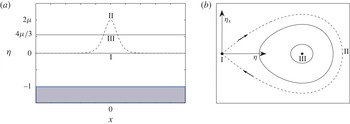
Sketches of the three unforced solutions,
 ${\it\epsilon}=0$
,
 ${\it\mu}>0$
. (a) Physical plane,
 $(x,{\it\eta})$
. The upper solid line is the uniform cnoidal stream solution III,
 ${\it\eta}(x)=4{\it\mu}/3$
. The lower solid line is the uniform stream solution I,
 ${\it\eta}(x)=0$
. The broken curve is the solitary wave solution II,
 ${\it\eta}(0)=2{\it\mu}$
. The shaded region,
 ${\it\eta}(x)\leqslant -1$
, is the flat channel bed. (b) Autonomous phase plane,
 $({\it\eta},{\it\eta}_{x})$
. The saddle point located at the origin is solution I. The centre located at
 $(4{\it\mu}/3,0)$
is solution III. The homoclinic orbit is solution II.

With
 ${\it\epsilon}=0$
, Binder et al. (Reference Binder, Dias and Vanden-Broeck2005) and others have shown that (1.1) can be expressed as a two-dimensional nonlinear dynamical system with two fixed points. The classification of the fixed points depends on whether
 ${\it\mu}<0$
or
 ${\it\mu}>0$
. If we initially restrict attention to the case when
 ${\it\mu}>0$
, the first of these points lies at the origin of the
 $({\it\eta},{\it\eta}_{x})$
phase plane and corresponds to a saddle point, as is illustrated in figure 1(b). It represents a uniform stream (herein termed solution I) with
 ${\it\eta}(x)=0$
. The homoclinic orbit connecting the fixed point at the origin to itself, seen as a broken line in figure 1(b), corresponds to the classical unforced solitary wave (solution II) given by
 $$\begin{eqnarray}{\it\eta}(x)=2{\it\mu}\text{sech}^{2}\left(\sqrt{\frac{3{\it\mu}}{2}}x\right).\end{eqnarray}$$
Both solution types I and II satisfy the far-field uniform flow condition (
 ${\it\eta}_{xx}\rightarrow 0$
,
 ${\it\eta}_{x}\rightarrow 0$
,
 ${\it\eta}\rightarrow 0$
as
 $x\rightarrow \pm \infty$
) used in the derivation of (1.1). The second fixed point is located at
 $({\it\eta},{\it\eta}_{x})=(4{\it\mu}/3,0)$
in the phase plane and corresponds to a centre. The closed trajectories centred around this fixed point are usually called cnoidal waves, and can be expressed in closed form using Jacobi elliptic functions (Billingham & King Reference Billingham and King2000). The second fixed point at
 ${\it\eta}=4{\it\mu}/3$
represents another constant-level solution, which we term a uniform cnoidal stream (solution III). This solution appears to lack physical relevance as it violates the far-field flow condition
 ${\it\eta}\rightarrow 0$
used in the derivation of (1.1). However, we note that if we perform the replacement
 $$\begin{eqnarray}{\it\eta}\rightarrow {\it\eta}+4{\it\mu}/3,\quad \text{followed by }{\it\mu}\rightarrow -{\it\mu},\end{eqnarray}$$
to (1.1), we recover the same equation. This invariance means that this second fixed point is associated with a solution satisfying
 ${\it\eta},{\it\eta}_{x},{\it\eta}_{xx}\rightarrow 0$
in the far field for a different
 ${\it\mu}$
value, and hence has physical relevance.
To retain consistency, we shall initially characterise all of the possible subtypes of perturbed solutions for the same value of
 ${\it\mu}>0$
. The unforced solutions I–III are shown in the physical plane in figure 1(a). When
 ${\it\sigma}(x)\neq 0$
, these three types of solutions – near-uniform, solitary and cnoidal – perturb. The focus of this article is to characterise exactly these forced solutions, for which we obtain explicit analytical wave profiles. We remark that our (1.1) and (1.2) are similar to those considered by Grimshaw & Tian (Reference Grimshaw and Tian1994), who demonstrated that the system possessed chaotic solutions. The forced solitary-type wave (type II) is the specific type of solution that leads to the presence of nearby chaotic solutions, in the sense that it corresponds exactly to the intersection of stable and unstable manifolds which is necessary to establish that the system is chaotic (Guckenheimer & Holmes Reference Guckenheimer and Holmes1983; Rom-Kedar, Leonard & Wiggins Reference Rom-Kedar, Leonard and Wiggins1990).
We compute numerical solutions of (1.1) using the scheme described in the supplementary material, appendix B. Typical elevation profiles for
 ${\it\mu}=0.1$
,
 $k=3.0$
and
 $|{\it\epsilon}|=0.1$
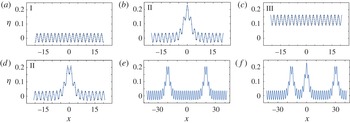
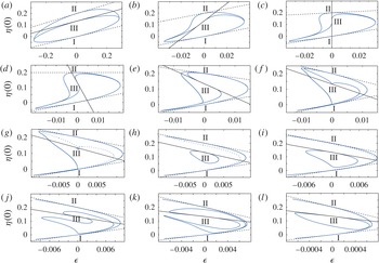
are presented in figure 2. Figure 3 shows the bifurcation structure for the case
 ${\it\mu}=0.1$
, in which the numerics show excellent correspondence with the analytical approximations for types I and II (derived in § 2), and type III (derived in § 3). In § 4, we further analyse the morphology of the solutions when
 ${\it\mu}>0$
, and consider two other types of forcing in a flow regime when
 ${\it\mu}<0$
.
2. Type I and II solutions: non-autonomous theory
The uniform stream and solitary wave solutions of the autonomous system (1.1) with no forcing are represented respectively by the fixed point at the origin and its homoclinic connection in figure 1(b). ‘Homoclinic’ means that branches of the stable and unstable manifolds of the fixed point coincide, and hence the associated wave approaches
 $({\it\eta},{\it\eta}_{x})=(0,0)$
as
 $x\rightarrow \pm \infty$
. Inclusion of the forcing term (i.e.
 ${\it\epsilon}\neq 0$
) renders the system non-autonomous. To understand this, we adapt the recently developed theory of Balasuriya & Binder (Reference Balasuriya and Binder2014), a detailed discussion of which is provided in the supplementary material, appendix C. For
 $|{\it\epsilon}|\ll 1$
, it can be shown that there is only one solution that remains
 $\mathit{O}({\it\epsilon})$
-close to the uniform stream (i.e. the saddle fixed point in figure 1
b) over the entire unbounded domain (Balasuriya Reference Balasuriya2011; Balasuriya & Padberg-Gehle Reference Balasuriya and Padberg-Gehle2013, Reference Balasuriya and Padberg-Gehle2014), and this is given by
 $$\begin{eqnarray}{\it\eta}^{I}(x)=\frac{3{\it\epsilon}\cos (kx)}{k^{2}+6{\it\mu}}\end{eqnarray}$$
to
 $\mathit{O}({\it\epsilon}^{2})$
. The dotted curves in figure 2(a) are for this near-uniform solution (2.1), which is the non-autonomous type I solution.
Next, we consider solutions that are near-solitary. These are solutions that have one big hump with a height of approximately
 $2{\it\mu}$
, overlaid with smaller oscillations, and that decay in the far field to the near-uniform solution (2.1). This is the only natural far-field possibility for near-solitary waves in this non-autonomous setting, since the only solution that remains approximately uniform as
 $x\rightarrow \pm \infty$
is (2.1). The dynamical-systems interpretation is that these are homoclinic trajectories to (2.1) which are near to a corresponding homoclinic trajectory to the autonomous system. When
 ${\it\epsilon}=0$
, an uncountable number of one-humped solitary waves are obtained by taking arbitrary shifts of (1.3). When
 $|{\it\epsilon}|\ll 1$
but is non-zero, the non-autonomous theory of Balasuriya & Binder (Reference Balasuriya and Binder2014) can be adapted to characterise all one-humped solitary waves. As derived in the supplementary material, appendix C, there are exactly two possible types of such one-humped solitary waves: (i) those centred around crests and (ii) those centred around troughs of the topography. Near-solitary waves within each of these two families are simple shifts of each other by multiples of
 $k{\rm\pi}$
. For example, if
 ${\it\epsilon}>0$
, there is a crest of
 ${\it\sigma}$
at
 $x=0$
, resulting in a crest-centred near-solitary wave centred at
 $x=0$
. Other crest-centred near-solitary waves can be obtained by shifting this to the values
 $x=2n{\rm\pi}/k$
,
 $n\in \mathbb{Z}$
. Trough-centred near-solitary waves would therefore be centred at
 $x=(2n+1){\rm\pi}/k$
,
 $n\in \mathbb{Z}$
. In contrast to the autonomous situation, there are only a countable number of such one-humped near-solitary waves. As described in the supplementary material, appendix C, these near-solitary waves are the only ‘regular’ structures among ‘nearby’ solutions which are well known to be chaotic (Grimshaw & Tian Reference Grimshaw and Tian1994), exhibiting seemingly random
 $\mathit{O}(1)$
excursions.
The one-humped non-autonomous near-solitary waves can be expressed to
 $\mathit{O}({\it\epsilon})$
explicitly by adapting the wave-profile theory of Balasuriya & Binder (Reference Balasuriya and Binder2014) which builds on the stable/unstable manifold determination in Balasuriya (Reference Balasuriya2011) as described in detail in the supplementary material, appendix C. The near-solitary wave centred at
 $x=0$
is given by
 $$\begin{eqnarray}{\it\eta}^{II}(x)=\bar{{\it\eta}}(x)+{\it\epsilon}[{\it\eta}^{n}(x)+{\it\eta}^{t}(x)]+\mathit{O}({\it\epsilon}^{2}),\end{eqnarray}$$
in which
 $\bar{{\it\eta}}$
is the fundamental solitary wave solution (1.3),
 $$\begin{eqnarray}{\it\eta}^{n}(x)=-\frac{3\bar{{\it\eta}}_{xx}(x)}{\bar{{\it\eta}}_{x}(x)^{2}+\bar{{\it\eta}}_{xx}(x)^{2}}\int _{|x|}^{\infty }\bar{{\it\eta}}_{x}({\it\tau})\cos (k{\it\tau})\,\text{d}{\it\tau}\end{eqnarray}$$
and
 $$\begin{eqnarray}{\it\eta}^{t}(x)=-3\bar{{\it\eta}}_{x}(|x|)\int _{0}^{|x|}\frac{\bar{{\it\eta}}_{xx}({\it\tau})\cos (k{\it\tau})-{\it\Omega}({\it\tau})\displaystyle \int _{|x|}^{\infty }\bar{{\it\eta}}_{x}({\it\lambda})\cos [k({\it\lambda}+{\it\tau}-x)]\,\text{d}{\it\lambda}}{\bar{{\it\eta}}_{x}({\it\tau})^{2}+\bar{{\it\eta}}_{xx}({\it\tau})^{2}}\,\text{d}{\it\tau},\end{eqnarray}$$
where
 $$\begin{eqnarray}{\it\Omega}({\it\tau}):=\frac{[6(1+{\it\mu})-9\bar{{\it\eta}}({\it\tau})-5][\bar{{\it\eta}}_{x}({\it\tau})^{2}-\bar{{\it\eta}}_{xx}({\it\tau})^{2}]}{\bar{{\it\eta}}_{x}({\it\tau})^{2}+\bar{{\it\eta}}_{xx}({\it\tau})^{2}}.\end{eqnarray}$$
The solution (2.2) is crest-centred if
 ${\it\epsilon}>0$
and trough-centred if
 ${\it\epsilon}<0$
. Waves centred at other
 $x$
-values can be computed from these solutions by simply shifting the wave solutions. The theoretical waves computed from (2.2) are virtually identical to the numerically computed solutions shown by the solid curves in figure 2(b,d). To demonstrate this visually for curves that virtually fall on top of one another, we show the theoretical solution values computed from (2.2) on a coarse grid, shown by dots in figure 2(b,d). The crest-centred solutions have an upwelling at the central crest, whereas the trough-centred ones have dips, as shown respectively in figure 2(b,d).
The single-humped solitary waves are, as is clear from (2.2), symmetric about their central value. The presence of different single-humped solitary waves means that many-humped ones will exist as approximately the sum of several of the single-humped ones: figure 2(e) is composed of two trough-centred ones, while figure 2(f) has two trough-centred and one crest-centred one. Indeed, these figures were numerically obtained by using such a sum as an initial guess. Therefore, it is possible to form multi-humped solitary waves that are not symmetric.
While the above expressions are messy, the height at the central crest/trough at
 $x=0$
can be derived to be (see the supplementary material, appendix C)
 $$\begin{eqnarray}{\it\eta}^{II}(0)=2{\it\mu}+\frac{{\it\epsilon}}{{\it\mu}}\left(k\int _{0}^{\infty }\text{sech}^{2}\left(\sqrt{\frac{3{\it\mu}}{2}}t\right)\sin (kt)\,\text{d}t-1\right).\end{eqnarray}$$
The lower and upper broken straight lines in the panels of figure 3 correspond to values given by (2.1) and (2.6) respectively, demonstrating that the near-uniform and near-solitary waves obtained from the non-autonomous theory show excellent agreement with the numerics.
The near-solitary waves derived in this section are obtained explicitly in the unbounded
 $x$
-domain for small topography, with no additional assumptions, matching conditions or enforced spatial periodicity. Following a genuinely non-autonomous viewpoint helped to avoid such assumptions, which are often used in similar fKdV equations (e.g. Ockendon et al.
Reference Ockendon, Ockendon and Johnson1986; Amundsen et al.
Reference Amundsen, Cox and Mortell2007).
Free-surface profiles,
 ${\it\mu}=0.10$
,
 $k=3.0$
,
 $|{\it\epsilon}|=0.1$
. The solid curves are numerical solutions. The dotted curve in (a) is for the non-autonomous approximation (2.1). The dotted curves in (b,d) are for the non-autonomous approximation (2.2). The dotted curve in (c) is for the asymptotic theory, retaining only the first term in the regular expansion (3.2). (a) Perturbation of a uniform stream solution I,
 ${\it\eta}(0)=0.036$
,
 ${\it\epsilon}=0.1$
. (b) Perturbation of a solitary wave solution II,
 ${\it\eta}(0)=0.231$
,
 ${\it\epsilon}=0.1$
. (c) Perturbation of a uniform cnoidal stream solution III,
 ${\it\eta}(0)=0.167$
,
 ${\it\epsilon}=0.1$
. (d) Perturbation of a solitary wave solution II,
 ${\it\eta}(0)=0.151$
,
 ${\it\epsilon}=-0.1$
. (e,f) Additional solutions,
 ${\it\epsilon}=0.1$
.

Bifurcation diagrams for the elevation of the free surface,
 ${\it\eta}(0)$
, versus the amplitude of forcing,
 ${\it\epsilon}$
, with
 ${\it\mu}=0.1$
. The solid curves are for the numerical solutions. The upper, middle and lower branches that emanate from the vertical axis correspond to perturbations of a uniform stream, solitary wave and uniform cnoidal stream solutions I–III. The dotted curves in (g–i) are additional numerical type III solutions, as indicated by the asymptotic theory. The lower and upper broken straight lines are for the non-autonomous approximations (2.1) and (2.6) respectively. The solid straight lines are for the asymptotic theory, retaining only the first term in the regular expansion (3.2). Wavenumber forcing: (a)
 $k=3$
, (b)
 $k=1$
, (c)
 $k=0.7746$
, (d)
 $k=0.69378$
, (e)
 $k=0.5$
, (f)
 $k=0.3878$
, (g)
 $k=0.387$
, (h)
 $k=0.346$
, (i)
 $k=0.3$
, (j)
 $k=0.25$
, (k)
 $k=0.1$
, (l)
 $k=0.05$
.

3. Type III solutions: asymptotic theory
As noted above, there exist unforced periodic cnoidal wave solutions to (1.1) when
 ${\it\epsilon}=0$
. To discuss the forced counterparts of such type III solutions we recast in terms of the shifted variable
 $N(x)={\it\eta}(x)-4{\it\mu}/3$
, in which case (1.1) becomes
 $$\begin{eqnarray}N_{xx}+{\textstyle \frac{9}{2}}N^{2}+{\it\nu}_{c}^{2}N=-3{\it\epsilon}\cos kx,\end{eqnarray}$$
where
 ${\it\nu}_{c}=\sqrt{6{\it\mu}}$
is the frequency of small-amplitude unforced cnoidal waves which arise when
 ${\it\epsilon}=0$
and
 $N\ll 1$
. It is now clear from (3.1) that resonance may occur for small-amplitude waves if
 $k={\it\nu}_{c}$
. Furthermore, nonlinear generation of higher harmonics via the second term on the left-hand side of (3.1) raises the prospect of secondary resonances at
 $k={\it\nu}_{c}/2^{n}$
for
 $n=2,3,4,\ldots$
. Grimshaw & Tian (Reference Grimshaw and Tian1994) discussed resonance for the fKdV equation in the presence of damping effects.
When
 $k\neq {\it\nu}_{c}/2^{n}$
, for
 $n\in \mathbb{N}$
, there is no resonance. In this case, for small-amplitude waves,
 $|{\it\epsilon}|\ll 1$
, we seek a solution as a regular expansion in the form
 $$\begin{eqnarray}N={\it\epsilon}N_{1}(x)+{\it\epsilon}^{2}N_{2}(x)+\cdots \,.\end{eqnarray}$$
Substituting into (3.1) and considering the linear problems obtained at each order of approximation, we may easily determine
 $N_{1}(x)$
,
 $N_{2}(x)$
, and so on. Indeed, we find
 $$\begin{eqnarray}N_{1}(x)=\frac{3\cos (kx)}{k^{2}-6{\it\mu}},\end{eqnarray}$$
which shows that small-amplitude waves are in phase with the topography for frequencies above resonance,
 $k>{\it\nu}_{c}$
, and are a half-period out of phase with the topography when
 $k<{\it\nu}_{c}$
(in contrast with the small-amplitude type I solution (2.1) which is always in phase with the topography). The dotted curve in figure 2(c) and the solid straight lines in the panels of figure 3 are for the asymptotic expansion (3.2), where we have retained only the first term in the expansion.
More interesting is the small-amplitude response at the resonant frequencies. At primary resonance,
 $k={\it\nu}_{c}$
, to obtain a bounded periodic solution, we expand in fractional powers of
 ${\it\epsilon}$
, writing
 $$\begin{eqnarray}N(x)={\it\epsilon}^{1/3}n_{1}(x)+{\it\epsilon}^{2/3}n_{2}(x)+{\it\epsilon}n_{3}(x)+\cdots \,.\end{eqnarray}$$
A key observation is that at second order,
 $\mathit{O}({\it\epsilon})$
, the first two terms in the expansion (3.4) will combine via the nonlinear term on the left-hand side of (3.1) to cancel the problematic forcing term on the right-hand side and thereby eliminate any secular terms. Indeed, at leading order
 $\mathit{O}({\it\epsilon}^{1/3})$
we find
 $n_{1}(x)=a_{1}\cos kx+b_{1}\sin kx$
, for constants
 $a_{1}$
and
 $b_{1}$
, and at first order
 $\mathit{O}({\it\epsilon}^{2/3})$
we obtain
 $$\begin{eqnarray}\displaystyle n_{2}(x) & = & \displaystyle a_{2}\cos kx+b_{2}\sin kx+\frac{3^{5/3}}{4}\frac{(a_{1}^{2}-b_{1}^{2})}{k^{2}}\cos 2kx\nonumber\\ \displaystyle & & \displaystyle +\,\frac{3^{5/3}}{2}\frac{a_{1}b_{1}}{k^{2}}\sin 2kx-\frac{3^{11/3}}{4}\frac{(a_{1}^{2}+b_{1}^{2})}{k^{2}},\end{eqnarray}$$
for constants
 $a_{2}$
and
 $b_{2}$
. At
 $\mathit{O}({\it\epsilon})$
we find that the term on the right-hand side of (3.1) is eliminated if
 $$\begin{eqnarray}a_{1}=\frac{2}{3^{2/3}5^{1/3}}k^{2/3},\quad b_{1}=0,\end{eqnarray}$$
and we obtain a periodic solution.
At the first secondary resonance, where
 $k={\it\nu}_{c}/2$
, we find that we must expand by writing
 $$\begin{eqnarray}N(x)={\it\epsilon}^{2/3}{\tilde{n}}_{1}(x)+{\it\epsilon}{\tilde{n}}_{2}(x)+{\it\epsilon}^{4/3}{\tilde{n}}_{3}(x)+{\it\epsilon}^{5/3}{\tilde{n}}_{4}(x)+{\it\epsilon}^{2}{\tilde{n}}_{5}(x)+\cdots \,.\end{eqnarray}$$
Working through the problems at successive orders of approximation, we find that
 ${\tilde{n}}_{1}(x)={\it\alpha}_{1}\cos 2kx+{\it\beta}_{1}\sin 2kx$
, for constants
 ${\it\alpha}_{1}$
and
 ${\it\beta}_{1}$
, and
 $$\begin{eqnarray}{\tilde{n}}_{2}(x)={\it\alpha}_{2}\cos 2kx+{\it\beta}_{2}\sin 2kx-\frac{1}{k^{2}}\cos kx,\end{eqnarray}$$
for constants
 ${\it\alpha}_{2}$
and
 ${\it\beta}_{2}$
. It is now evident that the quadratic nonlinearity in (3.1) will generate, via the second term in the expansion (3.7), a resonant forcing term proportional to
 $\cos {\it\nu}_{c}x\;(=\cos 2kx)$
at
 $\mathit{O}({\it\epsilon}^{2})$
. However, on noting that at next order we find
 $$\begin{eqnarray}{\tilde{n}}_{3}(x)={\it\alpha}_{3}\cos 2kx+{\it\beta}_{3}\sin 2kx+\frac{3^{1/3}}{5^{2/3}4k^{10/3}}(\cos 4kx-3),\end{eqnarray}$$
where
 ${\it\alpha}_{3}$
and
 ${\it\beta}_{3}$
are constants, it becomes clear that the problematic resonant term at
 $\mathit{O}({\it\epsilon}^{2})$
may be removed by virtue of the nonlinear interaction of the first and third terms in the expansion (3.7) and a judicious choice of the constants
 ${\it\alpha}_{1}$
and
 ${\it\beta}_{1}$
. Indeed, we find that the resonant term is eliminated if we choose
 $$\begin{eqnarray}{\it\alpha}_{1}=\frac{2}{3^{1/3}5^{1/3}k^{2/3}},\quad {\it\beta}_{1}=0,\end{eqnarray}$$
to yield a periodic solution. Other secondary resonances with
 $k={\it\nu}_{c}/4$
, and so on, can be dealt with similarly.
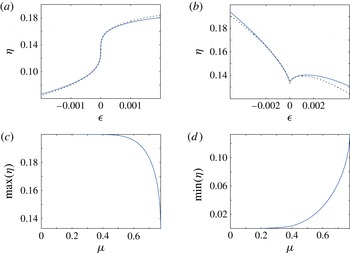
Analysis of cnoidal waves,
 ${\it\mu}=0.10$
. (a,b) Comparison of the type III computed solution branches (solid curves) with the asymptotic theory (dotted curves) for forcing wavenumbers
 $k=0.7746$
and
 $k=0.3873$
respectively. In (a) the first two terms in the expansion (3.4) have been used and in (b) the first three terms in the expansion (3.7) have been used. (c,d) Unforced cnoidal wave maxima/minima against wavenumber
 ${\it\nu}$
,
 ${\it\epsilon}=0$
. The wavenumber occupies
 $0\leqslant {\it\nu}\leqslant \sqrt{6{\it\mu}}=0.7746$
. (c) Wave maximum, with
 $4/3\leqslant \max ({\it\eta})\leqslant 0.2$
. (d) Wave minimum, with
 $0\leqslant \min ({\it\eta})\leqslant 4/3$
.

In figure 4 the expansions (3.4) and (3.7) are compared with numerical results at the primary resonance and first secondary resonance for
 ${\it\mu}=0.10$
. The asymptotic solutions (3.4) and (3.7) are shown as dotted curves in figure 4(a,b) respectively. In figure 4(a) the slope of the solution curve is infinite at
 ${\it\epsilon}=0$
, as is predicted by the asymptotic expansion (3.4), and in figure 4(b) the cusp predicted by (3.7) at
 ${\it\epsilon}=0$
is evident. The close overlap between the solid and the broken curves confirms good agreement between the asymptotic theory and the numerical computations. Furthermore, we find that the region of overlap between the solid lines and the broken lines broadens on including higher-order terms in the expansions.
To interpret the numerical results, it is helpful to consider the cnoidal wave solutions that are compatible with a given forcing wavenumber
 $k$
. In fact, for a chosen wavenumber
 $k$
, we would expect to obtain branches of periodic wave solutions that emerge continuously (as
 $|{\it\epsilon}|$
is increased) from unforced cnoidal wave solutions at
 ${\it\epsilon}=0$
if the cnoidal wavenumber,
 $m$
, is a rational multiple of
 $k$
, that is if
 $m=rk$
for
 $r\in \mathbb{Q}$
. If we restrict our numerical computations to a truncated domain containing just one wavelength, then we instead require either
 $r\in \mathbb{N}$
, giving superharmonic cnoidal waves, or
 $1/r\in \mathbb{N}$
, giving subharmonic cnoidal waves. To this end, it will be useful to consider the possible unforced cnoidal wave frequencies for given values of
 ${\it\mu}$
and
 $k$
. We restrict attention to superharmonic cnoidal waves, that is waves with wavelength a fraction of the forcing period, and assume that
 $r\in \mathbb{N}$
. To inform the discussion in the next section, we present in figure 4(c,d) the maxima and minima of the family of cnoidal waves obtained as periodic solutions to the fully nonlinear problem (3.1) for the case
 ${\it\mu}=0.1$
. The curves are plotted against the wavenumber
 ${\it\nu}$
. In the limit of small-amplitude cnoidal waves, corresponding to circuits tight around the point III in figure 1(b),
 $\max ({\it\eta})$
and
 $\min ({\it\eta})$
both approach the value
 $4{\it\mu}/3=1.333$
, and the wavenumber
 ${\it\nu}$
approaches the critical value
 ${\it\nu}_{c}=0.7746$
.
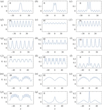
Free-surface profiles for
 ${\it\mu}=0.10$
: (a–c)
 $k=0.7746$
,
 ${\it\epsilon}=-0.0065$
; (a)
 ${\it\eta}(0)=0.171$
, (b)
 ${\it\eta}(0)=0.120$
, (c)
 ${\it\eta}(0)=0.043$
; (d–f)
 $k=0.69378$
,
 ${\it\epsilon}=0.0005$
; (d)
 ${\it\eta}(0)=0.187$
, (e)
 ${\it\eta}(0)=0.120$
, (f)
 ${\it\eta}(0)=0.070$
; (g–i)
 $k=0.3878$
,
 ${\it\epsilon}=0.005$
; (g)
 ${\it\eta}(0)=0.173$
, (h)
 ${\it\eta}(0)=0.131$
, (i)
 ${\it\eta}(0)=0.029$
; (j–l)
 $k=0.3$
; (j)
 ${\it\epsilon}=0.005$
,
 ${\it\eta}(0)=0.089$
, (k)
 ${\it\epsilon}=0.005$
,
 ${\it\eta}(0)=0.057$
, (l)
 ${\it\epsilon}=-0.0097$
,
 ${\it\eta}(0)=0.256$
; (m–q)
 $k=0.1$
,
 ${\it\epsilon}=0.006$
; (m)
 ${\it\eta}(0)=0.103$
, (n)
 ${\it\eta}(0)=0.0796$
, (o)
 ${\it\eta}(0)=0.0626$
, (p)
 ${\it\eta}(0)=0.044$
, (q)
 ${\it\eta}(0)=0.1225$
; (r)
 $k=0.1$
,
 ${\it\epsilon}=-0.006$
,
 ${\it\eta}(0)=0.2495$
.

4. Discussion
Here, we further discuss the morphology in the solution structure of figure 3, in particular the dependence on the wavenumber
 $k$
. The solid curves are for the numerical solutions with
 ${\it\mu}=0.10$
. The lower and upper broken straight lines are for the non-autonomous approximations (2.1) and (2.6) respectively. The solid straight lines are for the asymptotic theory, retaining only the first term in the regular expansion (3.2). We begin by discussing the branches that emerge from the three unforced solutions I–III in figure 3(a), where
 $k=3.0$
. For either
 ${\it\epsilon}<0$
or
 ${\it\epsilon}>0$
, the three branches I–III intersect at
 ${\it\epsilon}\approx -0.28$
and
 ${\it\epsilon}\approx 0.28$
respectively. The solutions on branches I and III with a wave crest at
 $x=0$
for
 $0<{\it\epsilon}\leqslant 0.28$
(e.g. figure 2
a,c) are the same as their corresponding solutions found on branches I and III with a wave trough at
 $x=0$
for
 $-0.28\leqslant {\it\epsilon}<0$
. For this value of
 $k=3.0$
, the crests and troughs of the free-surface elevation and forcing are in phase for both solutions I and III. Moreover, the flow type I solutions remain in phase with the topography for all values of
 $k$
.
We find two qualitatively different solutions on the branches of flow type II that emanate from
 ${\it\eta}(0)=2{\it\mu}$
in figure 3(a). For an amplitude of forcing
 ${\it\epsilon}>-0.03$
, the solutions are characterised by a maximum elevation at
 $x=0$
that coincides with a wave crest on the topography, close to the maximum elevation of the unforced solitary wave (figure 2
b). When
 ${\it\epsilon}<-0.03$
, the solutions are characterised by a trough at
 $x=0$
(figure 2
d). The two qualitatively different subtypes of solution II both have an overall shape that is characteristic of the unforced solitary wave with perturbations that are in phase with the channel bottom topography. A similar structure of solutions is found for higher values of the forcing wavenumber (not shown), with a corresponding increasing number of fluctuations to the overall solitary wave shape. In contrast, the number of fluctuations to the overall solitary wave shape of the type II solutions decreases as
 $k$
decreases.
At the resonant forcing wavenumber
 $k={\it\nu}_{c}\approx 0.7746$
, we expect a change in the solution structure with regard to the type III cnoidal solutions, as discussed in § 3. The solution space at this wavenumber is shown in figure 3(c). Perhaps the most notable feature is that for some values of
 ${\it\epsilon}<0$
there are three subtypes of solution II (figure 5
a–c), but only one subtype of type II solutions when
 ${\it\epsilon}>0$
. The vertical branch of type III solutions at
 ${\it\eta}=0$
was discussed in § 3 and successfully compared with the predictions of asymptotic theory.
When
 $k<{\it\nu}_{c}$
there exist non-flat cnoidal wave solutions at
 ${\it\epsilon}=0$
. Figure 3(d) shows the solution space at
 $k=0.69378$
, just below
 ${\it\nu}_{c}$
. It should be noticed that these type III solution branches connect with the vertical axis in figure 3(d) at three values of
 ${\it\eta}(0)$
, corresponding to a solution with a flat free surface (
 ${\it\eta}(0)=0.33$
), a solution with its maximum
 ${\it\eta}=0.185$
above the topography maximum at
 $x=0$
, and a third solution with its minimum
 ${\it\eta}=0.061$
above the topography maximum at
 $x=0$
(these maximum/minimum values can be read off the curves in figure 4
c,d). Sample type III periodic wave profiles are shown in figure 5(d–f) for small positive
 ${\it\epsilon}$
. Two of these have a free surface out of phase with the topography as
 ${\it\epsilon}\rightarrow 0$
, with a trough immediately above a topography crest (figure 5
e,f), while the other is in phase with a crest above a topography crest.
The solution space shown at
 $k=0.5$
in figure 3(e) is qualitatively similar to that shown in figure 3(d). A further structural change occurs at the first secondary resonance,
 $k={\it\nu}_{c}/2=0.3872$
, where a cusp is expected in the type III solution branch at
 ${\it\epsilon}=0$
(see figure 4). Figure 3(f) shows the solution space at
 $k=0.3878$
, just above the secondary resonance frequency. The near-formation of the cusp is clearly visible. It should be noted that there are still three qualitatively different type III solutions, but, as can be seen from figure 4(c,d), two of them have
 ${\it\eta}(0)$
very close to
 $0.2$
and
 $0$
respectively, and so their solution branches almost coincide with those found for the flow types I and II (figure 3
f). The wave profiles on the branches that almost overlie these type III branches around
 ${\it\epsilon}=0$
now have a smaller wave crest that is in phase with the topography (figure 5
h), with the larger wave crests being out of phase with the forcing.
When
 $k<{\it\nu}_{c}/2$
, according to the discussion in § 3, superharmonic unforced cnoidal wave solutions are possible at
 ${\it\epsilon}=0$
, and this suggests the appearance of further branches of solution. Indeed, just after the type III solution cusp forms at
 $k={\it\nu}_{c}$
, a closed loop of type III solutions is created immediately below
 ${\it\eta}=0.133$
. This loop grows in size as
 $k$
is lowered, as can be seen in figure 3(g–i). Figure 5(j,k) shows typical wave profiles on the closed-loop solution branch for figure 3(i). In all there are five type III solution branches emerging from
 ${\it\epsilon}=0$
in figure 3(g–i). Three of these branches are as shown: at
 ${\it\epsilon}=0$
they correspond to a flat free surface, with
 ${\it\epsilon}=0.133$
, and two superharmonic cnoidal waves of frequency
 ${\it\nu}=2k$
which are in phase with, and one half-period out of phase with, the topography respectively. The maxima and minima on these waves can be read from the curves in figure 4(c,d). These imply the presence of two further solution branches (not shown) emerging from unforced solutions at
 ${\it\epsilon}=0$
with values of
 ${\it\eta}(0)$
that are very close to
 $0.2$
and
 $0$
respectively. It should be noted that there is now only one subtype of solution for flow type II with
 ${\it\epsilon}<0$
(figure 5
l).
When
 $k<{\it\nu}_{c}/3=0.2582$
, further superharmonic unforced cnoidal waves come into play and herald the appearance of more solution branches in the
 $({\it\epsilon},{\it\eta}(0))$
plane. For example, at
 $k=0.25$
shown in figure 3(j) the closed loop has deformed to admit four unforced cnoidal wave solutions at
 ${\it\epsilon}=0$
. In total, there are seven unforced cnoidal wave solutions at this wavenumber, with non-flat solutions having frequencies of
 $k$
,
 $2k$
and
 $3k$
(in each case two waves are possible, either in or out of phase with the topography). According to figure 4(c,d) some of the corresponding solution branches emerge from values of
 ${\it\eta}(0)$
very close to
 $0.2$
and
 $0$
, and we have not attempted to delineate them in figure 3(j).
Reducing
 $k$
still further presents the possibility of more superharmonic cnoidal waves and further secondary resonances, increasing the complexity of the solution space. Figure 3(k) shows the solution space for
 $k=0.1$
, which lies below the next secondary resonance at
 $k={\it\nu}_{c}/4=0.1936$
. It should be noted that in this figure we only show the closed-loop solution branch, and ignore the numerous other branches that emerge from
 ${\it\epsilon}=0$
. Figure 5(m–p) shows type III typical wave profiles on the closed loop in figure 3(k).
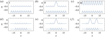
Free-surface profiles with
 ${\it\mu}=-0.3$
,
 $k=3.0$
,
 ${\it\epsilon}=0.06$
. (a–c) The topography is given by (4.1). (a) Perturbation of a uniform stream solution I. (b) Perturbation of a solitary wave solution II. (c) Perturbation of a uniform cnoidal stream solution III. (d–f) Additional solutions for compact topography given by (4.2),
 $m=3$
.

Although we have focused our attention on branches that emanate from the unforced solutions I–III, the non-autonomous theory indicates that there are infinitely many to be found. The numerical solutions in figure 2(e,f) are a case in point: they are approximately the superposition of several of the type II waves that we have analytically described, and were found by using such a superposition as an initial guess in the Newton iterative method.
The bifurcation structure of the cnoidal waves has particular relevance when considering
 ${\it\mu}<0$
. If so, the phase diagram for the unforced problem is the same as that shown in figure 1(b), but with a translation in
 ${\it\eta}$
of
 $4{\it\mu}/3$
to the left: the saddle is now at
 $(4{\it\mu}/3,0)$
, this has an attached homoclinic orbit with maximum
 ${\it\eta}=-2{\it\mu}/3$
, and the centre – the uniform cnoidal stream – is at
 $(0,0)$
. Since this satisfies the far-field conditions
 ${\it\eta}_{xx}\rightarrow 0$
,
 ${\it\eta}_{x}\rightarrow 0$
,
 ${\it\eta}\rightarrow 0$
as
 $x\rightarrow \pm \infty$
, the cnoidal stream (solution type III) is physically meaningful. On the other hand, the invariance as expressed in (1.4) shows the equivalence of this physical solution for
 ${\it\mu}<0$
and the uniform cnoidal stream for
 ${\it\mu}>0$
. Thus, our analysis of the cnoidal bifurcation structure for
 ${\it\mu}>0$
is directly applicable to the bifurcations of the physically relevant
 ${\it\mu}<0$
cnoidal waves.
Accordingly, we address
 ${\it\mu}<0$
in our next group of examples. First, we choose
 $$\begin{eqnarray}{\it\sigma}(x)={\it\epsilon}\left(\cos kx-\cos \left(\frac{kx}{2}\right)\right),\end{eqnarray}$$
for which numerical solutions are shown in figure 6(a–c). Comparison of the plots shown in figure 6(a–c) with those in figure 2(a–c) indicates that our method of analysis of the solution structure (e.g. figure 3) can be applied to other periodic topographies in either a
 ${\it\mu}>0$
or a
 ${\it\mu}<0$
flow regime.
The last example of forcing that we consider has compact support, given by
 $$\begin{eqnarray}{\it\sigma}(x)=\left\{\begin{array}{@{}ll@{}}\displaystyle {\it\epsilon}\left(\cos kx-\cos \left(\frac{kx}{2}\right)\right)\quad & \displaystyle \text{if }|x|\leqslant \frac{4{\rm\pi}m}{k}\\ 0\quad & \text{if else}\end{array}\right.,\end{eqnarray}$$
and the results presented in figure 6(d–f) can be viewed as type I, type II and combined type II solutions. In general, there are only finitely many near-solitary waves for compactly supported topography. Further examination of the solution structure in flows with
 ${\it\mu}\lessgtr 0$
for general forcing is left to future research, and we note that Binder, Blyth & Balasuriya (Reference Binder, Blyth and Balasuriya2014) considered the case of compact periodic forcing when
 ${\it\mu}=0$
.
5. Concluding remarks
We have studied solutions to the forced Korteweg–de Vries equation under periodic forcing as a model for the flow of water over a spatially periodic bed. We have computed new near-solitary wave solutions, which have periodic tails in the far field. Solutions with a peak of the solitary wave over each crest in the bed and solutions with a peak of the solitary wave over each trough in the bed are both possible. We have also found many bound-state solutions in the same flow which are approximately the superposition of several of these solitary-type waves. It is worth emphasising that in the unforced case (flat bed) the translational invariance of the KdV equation means that the classical
 $\text{sech}^{2}$
solution, given by (1.3), may be translated by an arbitrary amount to construct infinitely many acceptable solutions; however, it is not permissible to superpose two such solutions to form a multi-humped solution.
It is interesting to draw a connection between the new solutions discussed in the present work and known behaviour in the problem of resonant sloshing in a horizontally oscillating water tank (e.g. Ockendon et al. Reference Ockendon, Ockendon and Johnson1986; Amundsen et al. Reference Amundsen, Cox and Mortell2007). In the latter problem the fKdV equation arises in the limit of small-amplitude oscillations and shallow water. For the driving frequency close to resonance, Ockendon et al. (Reference Ockendon, Ockendon and Johnson1986) used an asymptotic analysis to obtain periodic solutions with very rapid and short-lived spiked bursts occurring at regular intervals in the time signal. Local solutions were constructed inside each of the rapid-burst regions; these solutions had a solitary-type character which was not dissimilar to those we have presented in figure 2 (see their figure 4, for example). We emphasise, however, that these local solutions form part of an overall periodic solution. Our solutions are of genuine solitary-type character, are non-periodic and have a clear physical interpretation in the context of flow over a corrugated bed.
We have left open here the issue of whether the solutions we have computed are stable or unstable, and work on this question is currently underway. The physical relevance of the new solitary-type solutions to fKdV that we have constructed must also be tested by seeking solutions of this type to the fully nonlinear water wave problem. This will also form the subject of a future investigation.
Acknowledgement
S.B. was supported by the Australian Research Council grant FT130100484.
Supplementary data
Supplementary data is available at http://dx.doi.org/10.1017/jfm.2015.507.