INTRODUCTION
Safflower (Carthamus tinctorius L.) is a member of the family Asteraceae (syn Compositae) cultivated mainly for its seeds as a source of oil, meal and birdseed. Historically, safflower was grown for its flowers, with the florets being used for colouring and flavouring of foods, for making dyes and as medicines (Johnston et al. Reference Johnston, Tanaka, Miller, Brandt, Nielsen, Lafond and Riveland2002). The oil can be used for both food, e.g. salad oil, margarine and frying oil, and non-food purposes such as paints, varnishes and coatings because genotypes with different fatty acid profiles exist (Knowles Reference Knowles1969). It is a deep-rooted annual crop that is grown mainly in arid and semiarid areas of the world. Safflower has wide adaptability to different climatic conditions and may grow on a wide range of soils (Esendal Reference Esendal, Corleto and Mündel1997). In Iran, safflower is usually cultivated after wheat in a crop rotation; it helps to decrease grass-type weeds and possibly disrupts plant pest and disease cycles that are common with monoculture. In addition, including safflower in wheat-based rotations can improve use of subsoil moisture and nutrients (Johnston et al. Reference Johnston, Tanaka, Miller, Brandt, Nielsen, Lafond and Riveland2002).
Current agronomic practice is for seeding in the cold northern regions of Iran to be generally carried out in spring, whereas in southern and temperate parts of Iran, where frost damage is minimal, spring-type safflower is planted from late autumn to late winter, resulting in higher yields. In Iran, most field experiments on safflower have shown that the influence of vernalization on flowering is not a limiting factor. Genotypes planted in spring did not show sensitivity to vernalization at any location.
Therefore, multi-environment trials (MET) are required to identify genotypes suitable for different areas and having the ability to yield across a range of geographic locations and, possibly, years (seasons).
The development of statistical methods for the analysis of MET data has a long history. Early methods were focused on analysis of variance (ANOVA) techniques that partitioned total variation into source due to genotypes, environments (location/year combination), the genotype×environment interaction (GEI) and within-trial error variation (Smith et al. Reference Smith, Cullis and Thompson2005). A major drawback with this approach is that it provides no insight into the nature of GEI (Kempton Reference Kempton1984). A significant GEI can be either qualitative (i.e. crossover type), where the direction of response of genotypes varies across environments, or quantitative (i.e. non-crossover type), where the responses of genotypes vary only in magnitude, but not in rank (Gail & Simon Reference Gail and Simon1985). Crossover interaction is the most intricate type of GEI with respect to identifying the best genotype(s) in a selection programme (Baker Reference Baker1988). When genotypes are selected for wide adaptation, plant breeders prefer the absence of GEI or a non-crossover interaction (Matus-Cádiz et al. Reference Matus-Cádiz, Hucl, Perron and Tyler2003). If there were no GEI relevant to a breeding objective, selection would be greatly simplified because the best genotype in one environment would also be the best genotype for all target environments (Basford & Cooper Reference Basford and Cooper1998).
Several parametric and non-parametric tests have been proposed to determine the statistical significance of GEI (Bredenkamp Reference Bredenkamp1974; Hildebrand Reference Hildebrand1980; De Kroon & Van Der Laan Reference De Kroon and Van Der Laan1981; Azzalini & Cox Reference Azzalini and Cox1984; Gail & Simon Reference Gail and Simon1985; Kubinger Reference Kubinger1986). The parametric statistical procedure of Azzalini & Cox (Reference Azzalini and Cox1984) tests the significance of G×E crossover interactions and involves calculating the difference between all pairs of genotypes in all possible pairs of environments (quadruples). Crossover interaction is present if there is at least one 2×2 (G×E) quadruple in which the difference between genotypes has opposite signs in the two environments. In a different approach, Gail & Simon (Reference Gail and Simon1985) proposed a maximum likelihood test to determine the significance of crossover interaction between two genotypes across a series of environments. Hühn & Léon (Reference Hühn and Léon1995) compared four non-parametric procedures of interactions and grouped them into two different concepts of interactions. While the Bredenkamp, Hildebrand and Kubinger procedures are based on deviations from additivity of main effects for genotypes and environments, the De Kroon & Van Der Laan (Reference De Kroon and Van Der Laan1981) method is based on the crossover interactions (i.e. different rank orders).
Statistics have also been developed to estimate the relative performance stability of genotypes across environments (Wricke Reference Wricke1962; Eberhart & Russell Reference Eberhart and Russell1966; Shukla Reference Shukla1972; Lin & Binns Reference Lin and Binns1988). Most of the parametric measures of stability are variance components or related statistics (Piepho & Lotito Reference Piepho and Lotito1992). These measures work well when the statistical assumptions, such as normal distribution of errors and interaction effects. Some authors (Hühn Reference Hühn1979; Kang Reference Kang1988; Fox et al. Reference Fox, Skovmand, Thompson, Braun and Cormier1990; Thennarasu Reference Thennarasu1995) have proposed non-parametric procedures that are based on the ranks of genotypes in each environment; genotypes with similar ranking across environments are classified as stable. According to Huehn (Reference Huehn1990), non-parametric procedures may be superior to parametric stability methods because they reduce the bias caused by outliers, no assumptions are required about the distribution of the observed values, they are easy to use and interpret; additions or deletions of one or more genotypes do not cause much variation in the estimates, and for many applications (e.g. selection in breeding and testing programmes), the rank order of genotypes is the most essential information.
Few studies of GEI and stability have been reported on safflower as a spring-sown crop. The objectives of the present study were: (i) to investigate the crossover and non-crossover interaction in an MET, (ii) to study the relationships among parametric and non-parametric stability statistics and (iii) to identify promising safflower genotypes by simultaneously assessing seed yield and stability in rain-fed areas of Iran.
MATERIALS AND METHODS
Multi-environment safflower trials
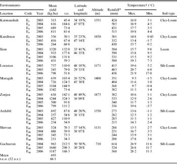
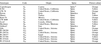
The present study was conducted using seed yield data from 17 safflower genotypes tested in 33 environments (year×location combinations during 2003–06) under rain-fed conditions. The characteristics of the trial locations are presented in Table 1. Nine locations were used for yield trials, i.e. Kermanshah, Kurdistan, Ilam and Lorestan in the west of Iran; Ardabil, Zanjan and Marageh in the east; Shirvan in the north east; Gachsaran in the south. In all test locations, yield trials were performed for 4 years except the trials at the Lorestan, Kurdistan and Gachsaran, which were conducted for 3 years. Genotypes were from the international safflower improvement programme based on a joint project between Iran and the International Center for Agricultural Research in the Dry Areas (ICARDA). The names, origin and characteristics of these genotypes are given in Table 2. At each environment, a randomized complete block design with three replications was used. Sowings in all locations took place on 15–30 March in each year.
Agro-climatic characteristics of the testing environments in Iran

* Total seasonal rainfall.
† Mean daily maximum & minimum temperature during the agronomic season (Oct–Jul) in each year.
Names, origin and characteristics of the 17 safflower genotypes studied in 33 environments (4 years and nine locations) in Iran

* Spiny leaves and bracts.
† The genotype Isfahan was the local control cultivar.
Sowing was carried out by hand in 1·5 m×4 m plots, consisting of 5 rows each 300 mm apart. Fertilizer application was 32 kg N/ha and 24 kg P2O5/ha at planting and 20 kg N/ha as a top dressing in early spring. Weeds were culled by hand about two or three times, as required. The trials were harvested when all the plants within each experimental plot had completely changed to straw colour. Seed yield per plot was obtained by harvesting the three-central rows of each plot (the area harvested was 3·6 m2) using a wheat plot-harvesting machine, after the appropriate screen adjustment. Data on seed yield were taken at 80 g/kg seed moisture level. Seed yield (kg/ha) was determined by converting the seed yields per plot into seed yields per hectare for the statistical analysis.
Statistical methods for testing the presence of G×E on yield
ANOVA
Combined ANOVA was conducted to determine the effects of genotype (G), environment (E) and interactions between the two (G×E). Statistical tests of significance for these factors were determined using F-tests.
Azzalini & Cox method
Truberg & Hühn (Reference Truberg and Hühn2000) used the method of Azzalini & Cox (Reference Azzalini and Cox1984) to evaluate a 2×2 sub-table for the presence of significant crossover interaction by using a value of t that gives a 5% experiment-wise error rate:

For each quadruple, the smallest absolute difference between genotypes is evaluated and the maximum (D) of all these absolute differences over all quadruples with sign reversals is used for the test procedure, and error probability α (type I error) is

where φ(−t) is the probability that a standard normal variable is less than −t, l is the number of genotypes, m is the number of environments and n is the number of replications.
Non-parametric methods
Three non-parametric statistical methods were also used to test the significance of GEI. The methods of Bredenkamp (Reference Bredenkamp1974) and Hildebrand (Reference Hildebrand1980) are based on the usual linear model for interaction: interactions are defined as deviations from the additivity of main effects. The procedure of De Kroon & Van Der Laan (Reference De Kroon and Van Der Laan1981) was used to test for crossover interaction. The three non-parametric statistical methods transform the original data into ranks and analyse the rank orders.
Bredenkamp method
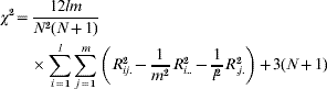
All Xijk values for all genotypes (i=1, 2, …, l), environments (j=1, 2, …, m) and replications (k=1, 2, …, n), are transformed into ranks Rijk of one single rank order. The test statistic for a test of GEI differences were calculated as follows:
Hildebrand method
The Xijk values are transformed  . The X*ijk values are ranked into a single rank order. The test statistic for a test of GEI differences was calculated as follows:

De Kroon & Van Der Laan method
The Xijk values for each environment are ranked separately into the ranks Rijk. The test statistic for the hypothesis that no genotypes change rank between environments (crossover interaction) was calculated as follows:

The test statistics of the above methods are approximately χ2-distributed with (l−1)(m−1) degree of freedom for a test of G×E, and N=lmn.
Statistical methods for testing the stability of yield
Parametric measures of stability
In the present study, several parametric methods of stability were used for measuring the stability of safflower genotype performance across environments: environmental variance (S xi2), ecovalence (W i; Wricke Reference Wricke1962), the coefficient of regression (b i), and the residual mean square of deviations from the regression (S di2; Eberhart & Russell Reference Eberhart and Russell1966). Eberhart & Russell (Reference Eberhart and Russell1966) regressed the mean yield of a genotype at a site on the mean yield of all varieties at a site and suggested the linear regression coefficient (b i) and deviation from linear regression (S di2) as parameters to estimate stability. According to the model, b i values approximating one coupled with S di2 of zero indicate average stability. Regression values that are significantly greater than unity describe genotypes with higher sensitivity to environmental changes and specific adaptation to favourable conditions. On the other hand, b i values that are significantly less than unity show lack of response to changes in environment and consistent performance for seed yield. They have a better adaptability to poor environments. The formulae of the various methods have previously been reviewed by Lin et al. (Reference Lin, Binns and Lefkovitch1986) and Becker & Léon (Reference Becker and Léon1988). The regression coefficients were tested for any significant difference from unity using the t-test, while the significance of the deviations of regression from zero was tested by the F-test.
In addition to these methods, superiority index (P i; Lin & Binns Reference Lin and Binns1988) was calculated using the highest-yielding genotype within each environment as a reference point. Higher-yielding genotypes have the smallest yield difference from the reference genotype and so have the lowest P i-values. These genotypes with lower values of P i are superior in yield to those with higher P i-values.
Non-parametric measures of stability
For a two-way data set with l genotypes and m environments, rij is denoted as the rank of the ith genotype in the jth environment,  as the mean rank across all environments for the ith genotype, r*ij is the rank of the adjusted value
 ,
 and M di* are the mean and median ranks for adjusted values. The genotype with the highest yield was given a rank of 1 and that with the lowest yield was assigned a rank of l.
Four sets of non-parametric statistics were used, based on yield ranks of genotypes in each environment to estimate stability. One of them consisted of four stability statistics (S i(1), S i(2), S i(3) and S i(6); Hühn Reference Hühn1979; Nassar & Hühn Reference Nassar and Hühn1987). Their equations are
S i(1), the mean of the absolute rank differences of a genotype over m environments:

S i(2), the variance among the ranks over the environments:
S i(3), the sum of the absolute deviations of rank for each genotype relative to the mean of ranks:
S i(6), the sum of squares of rank for each genotype relative to the mean of ranks:

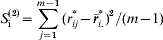
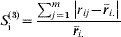
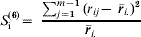
The significance test for the S i(1) and S i(2) statistics were suggested by Nassar & Hühn (Reference Nassar and Hühn1987). The chi-square (χ2) values associated with S i(1) and S i(2) were obtained using the expression  , where m=1, 2, Z i(m)=[S i(m)−E(S i(m))]/v(S i(m)), E(Si (m )) =expected value (=mean) of S i(m ) and v(S i(m) )=S i(m) variance.
Thennarasu (Reference Thennarasu1995) proposed another set of non-parametric statistics (NPi(1), NPi(2), NPi(3) and NPi(4)), based on ranks of adjusted means of the genotypes in each environment, and defined stable genotypes as those whose position remained unaltered in relation to the others in the set of environments assessed. These were calculated as follows:
NPi(1)
NPi(2)
NPi(3)
NPi(4)
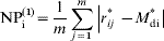
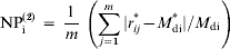
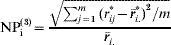

In Kang's (Reference Becker and Léon1988) Rank-Sum (RS) method, yield and Shukla's stability variance are the selection criteria. A weight is assigned to both yield and stability, with both the highest-yielding genotypes and the genotype with the lowest stability variance are ranked 1. Then, after ranking all the genotypes, the two sets of ranks are added for each genotype. The genotype with the lowest RS value is considered the most desirable.
Fox et al. (Reference Fox, Skovmand, Thompson, Braun and Cormier1990) proposed a non-parametric superiority measure for general adaptability using stratified ranking of cultivars. The proportion of environments in which the genotype occurred in the top third of the ranks was computed. Genotypes most often within the top third were considered as widely adapted genotypes.
Spearman rank correlations were used to evaluate relationships between different stability measures and seed yield. Principal component analyses (PCAs) based on the correlation matrix was performed to obtain an understanding of the relationships among stability measures.
RESULTS
Environments
The mean performance of seed yield over environments indicated the relative performance of the genotypes tested across environments (Table 1). The mean yield of environments ranged from 211 kg/ha (Shirvan 2006) to 1679 kg/ha (Gachsaran 2005). This yield range reflected the different climatic conditions across locations and years. Environmental mean yield was positively related to rainfall (r=0·58, P<0·01). Kurdistan 2006, Ardabil 2004 and 2006, and Shirvan 2006 were the lowest yielding environments, whereas Ilam 2003, Marageh 2006 and Gachsaran 2005 were the highest yielding environments. The highest yield (2118 kg/ha) was obtained with Cyprobregon at Gachsaran in 2005. The next best yielding genotypes were PI-537598 and Isfahan, grown at Gachsaran in 2005. The lowest yield (152 kg/ha) was given by PI-537636 grown at Ardabil in 2006.
The different statistical tests
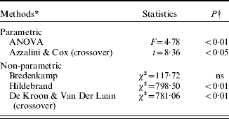
The combined ANOVA for the seed yield of safflower genotypes across environments showed that effects of genotype (G), environment (E) and GEI were highly significant. The partitioning of the sum of squares of the components indicated that G, E (year-location combinations) and GEI accounted for 0·01, 0·80 and 0·12 of the total variation, respectively. The Azzalini & Cox (Reference Azzalini and Cox1984) test revealed significant G×E crossover interaction for the quadruples of two of the genotypes and two of the environments (Table 3). Results of the different non-parametric statistical procedures also showed that the rank-interaction effects had a different pattern, while the Hildebrand (Reference Hildebrand1980) and the De Kroon & Van Der Laan (Reference De Kroon and Van Der Laan1981) methods revealed the same level of significance; the Bredenkamp (Reference Bredenkamp1974) method did not detect any difference in interaction effects (Table 3) and its χ2 value was the lowest. Hühn & Léon (Reference Hühn and Léon1995) also found non-significant χ2-values using the Bredenkamp method on several crop data sets. Also the De Kroon & Van Der Laan method showed lower χ2 value than the Hildebrand method. The results of the Azzalini & Cox and De Kroon & Van Der Laan analyses were in agreement with those from ANOVA, but provided more specific information about the nature of GEI.
Results of the different statistical methods for testing the presence of GEI in seed yield of 17 safflower genotypes grown in 33 environments (4 years and nine locations) in Iran
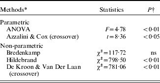
* The null hypothesis for ANOVA, Bredenkamp and Hildebrand is no non-crossover GEI and for Azzalini & Cox and De Kroon & Van Der Laan is no crossover GEI.
† ns=P>0·05.
Parametric measures of stability
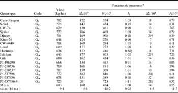
The mean performance and the stability analysis for the parametric statistics are given in Table 4. The mean seed yield of all genotypes across environments ranged from 629 to 772 kg/ha and the overall mean seed yield was 693 kg/ha. Environmental variance (S xi2) of genotypes detects all deviations from the mean seed yield. Genotypes with low S xi2 values under different environments are considered more stable than the others. The most stable genotypes were Hartman, Kino-76, CW-74 and PI-198290 although they had lowest yields. Genotypes PI-537636-S, Syrian and PI-537598 that had the highest yields were considered unstable.
Mean seed yield and parametric stability measures of seed yield for 17 safflower genotypes grown in 33 environments (4 years and nine locations) in Iran

* Environmental variance (S xi2), ecovalance (W i), regression coefficient (b i), deviation from regression (S di2) and superiority index (P i).
† S di2 values significantly different from zero at the 0·01 probability levels by F-test.
‡ b i value significantly different from unity at the 0·05 probability level by t test.
§ S di2 values significantly different from zero at the 0·05 probability levels by F-test.
Wricke (Reference Wricke1962) proposed the use of ecovalence, which measures the contribution of each tested genotype to GEI by partitioning it into variance components assignable to each genotype. Genotypes with lower ecovalence (W i) were considered to be stable. The W i values ranged from 191×103 (PI-250536) to 908×103 (Dincer). The most stable genotypes according to the ecovalence method were PI-250536, Lesaf, Kino-76 and CW-4440. Genotypes PI-250536 and CW-4440 showed yield performances above average. Genotypes Dincer and Isfahan had higher W i values, indicating lower stability.
An analysis following the Eberhart & Russell (Reference Eberhart and Russell1966) model showed that the linear regression coefficients of all genotypes (except Hartman) were not significantly different from unity. Hartman had b i significantly less than 1·00 thus showing specific adaptability to poor environments. Most of the genotypes (except Dincer, Isfahan, G17 and G15) showed deviation from linear regression (S di2) not significantly different from zero (S di2). Genotypes Dincer, Isfahan, PI-537636-S and PI-537598 with S di2 values significantly greater than zero, would have low predictability. Genotypes S-541, Syrian, PI-250536, CW-4440, PI-250537 and Cyprobregon showed yield performances above average, b i close to unity and deviation not significantly different from zero. Therefore, they had an average capacity for adaptation to all the environments. The yield performance of genotypes Lesaf, Gila, PI-537636, PI-198290, Kino-76 and CW-74 were below average, b i close to unity and deviation not significantly different from zero. Thus, these genotypes could be stable, but with low seed yield.
Lin & Binns (Reference Lin and Binns1988) suggested the use of stability index P i when describing the performance of one genotype across a range of environments. The superiority index of genotypes tested showed genotypes PI-250537, PI-250536, PI-537598 and CW-4440 had the highest stability; whereas CW-74, Hartman and Isfahan were the least stable ones.
Non-parametric measures of stability
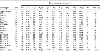
The estimates of non-parametric stability statistics are given in Table 5. The S i(1) (mean absolute rank differences) and S i(2) (variance of ranks) statistics of Hühn (Reference Hühn1979) are based on adjusted ranks of the genotypes across environments and they give equal weight to each environment. Genotypes with fewer changes in rank are considered to be more stable (Becker & Léon Reference Becker and Léon1988). According to Huehn (Reference Huehn1990) the use of S i(1) was preferred to S i(2) for many practical applications; it was reported to be easy to calculate and allows a clear and relevant interpretation. In the present study, the S i(1) and S i(2) statistics were not significant. Because the two overall Z i(1) and Z i(2) values (χ Sum2=16·0) were less than the critical χ2 value (26·31 for d.f.=16 and P=0·05). However, the individual Z-values for genotypes Syrian and Gila were significant because they showed large Z-values, in comparison with the critical χ2 value (3·84 for d.f.=1 and P=0·05). Hence, there was sufficient evidence for significant differences in stability between these two genotypes. While Gila had the smallest changes in rank and thus is regarded as the most stable genotype, Syrian was significantly unstable. Two other non-parametric statistics of Hühn (Reference Hühn1979)S i(3) and S i(6) combine yield and stability based on yield ranks of genotypes in each environment. These parameters measure stability in units of the mean rank of each genotype. The lowest value for each of these statistics indicates maximum stability for a certain genotype. Based on S i(3), genotypes Kino-76, CW-74, Hartman and Gila were the most stable, although had low mean yield performances, while genotypes Syrian, CW-4440 and PI-537598 were the least stable. As with S i(3), genotypes Kino-76, CW-74, Hartman and Gila were the most stable according to the S i(6) parameter, whereas PI-537598, Syrian and G7 were the most unstable.
Non-parametric stability measures for seed yield of 17 safflower genotypes grown in 33 environments (4 years and nine locations) in Iran

* Hühn's statistics (S i(1), …, and S i(6)), Thennarasu's statistics (NPi(1), …, and NPi(4)), Kang's RS, Fox et al. method (TOP).
† The Z i(1) and Z i(2) values are significant at the 0·05 probability level by χ2 test.
‡ P<0·05.
Thennarasu's (Reference Thennarasu1995) non-parametric stability statistics are calculated from ranks of adjusted yield means and genotypes with the lowest value are considered more stable. According to the first method (NPi(1)), genotype Gila was stable in comparison with other genotypes, followed by Kino-76, PI-250537 and S-541. The most unstable genotype according to NPi(1) statistic was Syrian, which ranked fourth for mean yield. Based on values of NPi(2) genotypes Gila), Kino-76, Isfahan and CW-74 had the lowest values and were therefore considered highly stable, although they had low mean yield performances. Stability parameters NPi(3) and NPi(4) identified Gila, CW-74, Kino-76 and Isfahan as the most stable genotypes. The most unstable genotype based on NPi(2), NPi(3) and NPi(4) was PI-537598, although it had the highest mean yield performance.
Kang's (Reference Kang1988) non-parametric stability parameter (RS) uses both yield and stability variance (Shukla Reference Shukla1972). The genotype with the lowest RS is the most favourable one; in the present study this was found to be PI-250536, followed by CW-4440. The genotypes with the highest RS were found to be Isfahan and CW-743.
The non-parametric superiority parameter of Fox et al. (Reference Fox, Skovmand, Thompson, Braun and Cormier1990) is obtained by scoring the proportion of environments in which each genotype ranked in the top third of trial entries. Thus, PI-537598 was found to be stable (high TOP value, 0·55 of all environments), and was followed by S-541 and Syrian in 0·46 and 0·42 of the environments, respectively. The least desirable genotypes were identified as CW-74, Kino-76 and Hartman.
Rank correlation among stability statistics and yield
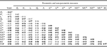
The results of the Spearman's rank correlation coefficient among the 15 parametric and non-parametric stability statistics and mean seed yield are presented in Table 6. Mean seed yield performance across environments was significantly positively correlated with b i, P i, RS and TOP measures (P<0·01), but it was not correlated with W i, S di2, S i(1), S i(2) and NPi(1). However, there were significant negative correlations between mean yield and S xi2, S i(3), S i(6), NPi(2), NPi(3) and NPi(4) (P<0·01). The high correlation between mean yield and stability measures is expected as the values of these statistics were higher for high yielding genotypes. The non-significant correlation and negative significant correlation between yield and stability parameters suggest that stability parameters provide information that cannot be gleaned from average yield alone (Mekbib Reference Mekbib2002).
Spearman rank correlation coefficients between seed yield and stability statistics

* Critical values of correlation P<0·05 and P<0·01 are 0·48 and 0·61, respectively. Values significantly different from 0·00 are in bold.
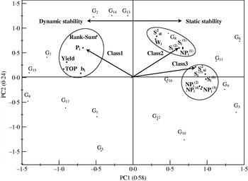
To better understand the relationships among parametric and non-parametric statistics, a principle component (PC) analysis based on the rank correlation matrix was performed on the 15 stability measures. The first two PCs explained 0·81 of the variance of the original variables (0·58 and 0·24 by PC1 and PC2, respectively).
The relationships among the different stability statistics are graphically displayed in a plot of PC1 and PC2 (Fig. 1). In this plot, three groups of stability statistics could be identified: Group 1 comprising Yield, b i, P i, RS, TOP; Group 2 comprising W i, S di2, S i(1), S i(2), NPi(1) and Group 3 comprising S xi2, S i(3), S i(6), NPi(2), NPi(3), NPi(4).
Plot of the first two PCs (PC1 v. PC2) of ranks of stability of yield, estimated by 15 methods using yield data from 17 safflower genotypes grown in 33 environments (4 years and nine locations) in Iran.

DISCUSSION
GEI becomes important when the rank order of breeding lines changes in different environments. This change in rank has been defined as a crossover GEI (Baker Reference Baker1988). In general, when different genotypes of a given crop are evaluated in a sufficiently wide range of environments, a crossover type of GEI is very common. Examples of crossover type of GEI can be found in the literature in a range of crops and environments, e.g. Ceccarelli (Reference Ceccarelli1989) in barley, Virk & Mangat (Reference Virk and Mangat1991) in pearl millet, Mason et al. (Reference Mason, Goonewardene and Spaner2008) in wheat, Truberg & Hühn (Reference Truberg and Hühn2000) in several data sets of oilseed rape, faba been, oat, fodder beet and sugar beet, Krishnan & Surya Rao (Reference Krishnan and Surya Rao2005) in rice, Laurentin et al. (Reference Laurentin, Montilla and Garcia2007) in sesame and Phakamas et al. (Reference Phakamas, Patanothai, Pannangpetch, Jogloy and Hoogenboom2008) with peanut. Smith et al. (Reference Smith, Cullis and Thompson2005) have provided an overview of current mixed model approaches for the analysis of crop cultivar breeding and evaluation trials.
Statistical tests of significance indicated that both significant non-crossover and crossover interactions were found in the present MET as judged by ANOVA, the Hildebrand procedure (for non-crossover or usual interaction) and the Azzalini & Cox and the De Kroon & Van Der Laan tests (for crossover interaction). The Bredenkamp method was not good at identifying deviations from additivity of main effects. Similar results were reported by Truberg & Hühn (Reference Truberg and Hühn2000) who instead recommended the Hildebrand test for usual interaction and the Azzalini & Cox and the De Kroon & Van Der Laan tests for crossover interaction. Truberg & Hühn (Reference Truberg and Hühn2000) found that the Azzalini & Cox approach is more sensitive for the detection of crossover interactions than the De Kroon & Van Der Laan procedure.
To identify cultivars with high and stable performances across a set of environments, each cultivar can be characterized by its yield stability parameter. There are different concepts of stability and a large number of different stability measures have been proposed (Lin et al. Reference Lin, Binns and Lefkovitch1986; Becker & Léon Reference Becker and Léon1988). The static concept of stability means that a genotype has a stable performance across environments and there is no between-environment variance. This would mean that a genotype would not respond to high levels of inputs. This type of stability would not be beneficial for the farmer, and it has been referred to as the biological concept of stability (Becker Reference Becker1981), which is equivalent to the type 1 stability of Lin et al. (Reference Lin, Binns and Lefkovitch1986). In type 1 stability, a genotype is regarded as stable if its between-environment variance is small. This is similar to the concept of homoeostasis widely used in quantitative genetics (Becker & Léon Reference Becker and Léon1988). The dynamic concept of stability means that a genotype has a stable performance, but, for each environment, its performance corresponds to the estimated or predicted level. This concept has been referred to as the agronomic concept (Becker Reference Becker1981), which is equivalent to Lin et al.'s (Reference Lin, Binns and Lefkovitch1986) type 2 stability. In type 2, a genotype is regarded as stable if its response to environments is parallel to the mean response of all genotypes in the trial.
When the various methods were compared using a PCA, the distribution of the methods on the first two PCs suggested the stability parameters could be divided into three distinct classes based on the two different concepts of stability: Fig. 1 shows, on the left, methods corresponding to the agronomic concept and, on the right, the methods based on the biological concept of stability. The mean yield was included in class 1 with P i (Lin & Binns Reference Lin and Binns1988), b i (Eberhart & Russell Reference Eberhart and Russell1966), TOP (Fox et al. Reference Fox, Skovmand, Thompson, Braun and Cormier1990) and RS (Kang Reference Kang1988) parameters, suggesting class 1 comprises those methods where yield has an important influence on the ranking across environments. Flores et al. (Reference Flores, Moreno and Cubero1998) considered that the P i and TOP procedures are associated with mean yield and the dynamic concept of stability. Kang & Pham (Reference Kang and Pham1991) found that the P i and RS methods are related to high yield performance, and therefore these stability parameters defined stability with dynamic concept. Similar results reported that selection based on P i (Sabaghnia et al. Reference Sabaghnia, Sabaghpour and Dehghani2008), P i and TOP (Mohammadi & Amri Reference Mohammadi and Amri2008) would favour selection for yield. The class 2 stability statistics, comprising Wrick's (Reference Wricke1962) ecovalence (W i), was strongly correlated with S di2 (Eberhart & Russell Reference Eberhart and Russell1966) and the S i(1) and S i(2) non-parametric methods of Hühn (Reference Hühn1979), which were strongly correlated with NPi(1) (Thennarasu Reference Thennarasu1995). These stability parameters, which were not associated with the yield level, were identified with the static concept of stability. Nassar & Hühn (Reference Nassar and Hühn1987) also reported that the S i(1) and S i(2) are associated with the static concept of stability, as they defined stability in the sense of homoeostasis. Piepho & Lotito (Reference Piepho and Lotito1992) also found a significant correlation between W i and S di2 and between S i(1) and S i(2). Other authors have reported high rank correlations of S i(1) and S i(2) (Flores et al. Reference Flores, Moreno and Cubero1998), which represent the static concept of stability. The S i(3) and S i(6) non-parametric methods of Hühn (Reference Hühn1979), three NPi statistics (NPi(2), NPi(3) and NPi(4)) of Thennarasu (Reference Thennarasu1995) and environmental variance (S xi2) were clustered together as class 3. Unlike class 1, these methods were strongly negatively correlated with seed yield. Nassar & Hühn (Reference Nassar and Hühn1987) pointed out that the S xi2 is associated with the static or biological concept of stability. Mohammadi & Amri (Reference Mohammadi and Amri2008) also found high rank correlations among S i(3), S i(6), NPi(2), NPi(3) and NPi(4) and similar with S xi2, which represents the static concept of stability.
Genotype evaluation under variable environments and adoption of simultaneous selection for yield and stability is the most valuable selection index that can be used in any plant breeding programme. It is concluded that the parametric and non-parametric measures including P i (Lin & Binns Reference Lin and Binns1988), b i (Eberhart & Russell Reference Eberhart and Russell1966), TOP (Fox et al. Reference Fox, Skovmand, Thompson, Braun and Cormier1990) and RS (Kang Reference Kang1988) would be useful to select high yielding and stable genotypes; therefore, these stability parameters defined stability with dynamic (agronomic) concept. However, in the present study, the heterogeneity of b i values was not significant (except for Hartman) and slope was therefore ignored. Of the 17 genotypes tested, the high yielding and stable genotypes (located in dynamic region of the plot) were PI-537598, CW-4440 and S-541.
As a result of the current analyses, the genotype PI-537598 was released for use in rain-fed conditions in Iran, as it adequately demonstrated stable and good yield performance, along with good seedling establishment under rain-fed conditions, medium height, a high number of capitula, mid to late maturing and a high oil content).
This research was part of a Regional Safflower Research Project of Dry-land Agricultural Research Institute (DARI) of Iran and Sponsored by the Agricultural Research and Education Organization (AREO). We thank all members of the project for any contribution they may have made towards this study.