


1. Introduction
Insurance firms operating under regimes such as Solvency II have the option to calculate their Solvency Capital Requirements (SCR) using an approved internal model, which in turn often relies on Monte Carlo simulation techniques to produce a distribution of future outcomes. These internal models often make use of outputs from so-called external models such as Economic Scenario Generators (ESGs) or Natural Catastrophe models. External models are used to supplement the internal model in areas where the firm’s own internal data, expertise, or resources are not sufficient to design, calibrate and maintain an appropriate model.
The output from external models arrives “pre-simulated” from the point of view of the internal model, in that it is usually a table of fixed numbers with a column for each variable and a simulation trial in each row. The joint distribution implicit in the external model output must be preserved. In other words, the columns in the table cannot be reordered independently of one another, and the consistency of each row in the table must be maintained.
This presents a challenge, as we often wish to specify and model various dependence relationships between variables in the external models and the internal model. This is becoming increasingly important given the interconnected nature of the modern world, the links between financial markets and physical phenomena, and the growing impact of climate change uncertainty. However, the only way that we can induce dependencies with a set of pre-simulated figures is to change their order relative to the variables in the internal model.
To model a dependency between a set of external model output and the internal model, apparent standard practice is to specify a single bivariate copula between one variable in the pre-simulated data and one in the internal model. This has various limitations, not least of which is that this can result in unintended and difficult-to-control dependencies between other pairs of variables, but no parameters to control these relationships.
This article therefore introduces a novel method that goes some way to resolving this problem, allowing actuaries to specify and achieve additional dependencies between pairs of variables in sets of pre-simulated data and the internal model.
2. Industry standard approach
In this section, we establish what I refer to as the industry standard approach and demonstrate a major limitation inherent in its use.
Let
 ${{\bf{X}}_A}$
be a set of pre-simulated variables from an external model, with
 $k$
observations of
 $m$
variables
 $\left\{ {{x_1}, \ldots, {x_m}} \right\}$
and correlation matrix
 ${R_A}$
. We wish to preserve the joint distribution of
 ${{\bf{X}}_A}$
exactly, and we therefore will not re-order the sample relative to itself. This may be because the sample is drawn from an external model such as an ESG or a Natural Catastrophe model. Let
 ${{\bf{X}}_B}$
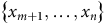
be a set of pre-simulated data from an internal model with
 $k$
observations of
 $\left( {n - m} \right)$
variables
 $\left\{ {{x_{m + 1}}, \ldots, {x_n}} \right\}$
and correlation matrix
 ${R_B}$
. As above,
 ${{\bf{X}}_B}$
has a joint distribution that we want to preserve. Assume that the samples for
 ${{\bf{X}}_A}$
and
 ${{\bf{X}}_B}$
are generated independently. In the event that we make no further assumptions, the joint density can then be written as the product of the densities:
 $${f_{AB}}\left( {{x_1}, \ldots, {x_n}} \right) = {f_A}\left( {{x_1}, \ldots, {x_m}} \right){\rm{\;}}{f_B}\left( {{x_{m + 1}}, \ldots, {x_n}} \right)$$
If we wish to induce dependence between variables in
 ${{\bf{X}}_A}$
and
 ${{\bf{X}}_B}$
, industry standard practice is to specify a single bivariate copula between one pair of variables
 $\left\{ {{X_i},{X_j}} \right\},i \in A,j \in B$
. A copula
 $C$
is a distribution on the unit square with standard uniform marginals, and a joint distribution can be expressed in terms of a copula distribution function
 $C$
as follows (Sklar, Reference Sklar1959):
 $${F_{1 \ldots n}}\left( {{x_1}, \ldots, {x_n}} \right) = {C_{1 \ldots n}}\left[ {{F_1}\left( {{x_1}} \right), \ldots, {F_n}\left( {{x_n}} \right)} \right]$$
with joint density:
 $${f_{1\ldots n}}\left( {{x_1},...,{x_n}} \right) = {c_{1...n}}\left[ {{F_1}\left( {{x_1}} \right),...,{F_n}\left( {{x_n}} \right)} \right] \cdot \mathop \prod \limits_{i = 1}^n {f_i}\left( {{x_i}} \right)$$
If we specify a bivariate copula with distribution function
 ${C_{ij}}$
and density
 ${c_{ij}}$
between some
 ${X_i},i \in A$
and some
 ${X_j},j \in B$
then the joint density becomes:
 $${f_{AB}}\left( {{x_1}, \ldots, {x_n}} \right) = {f_A}\left( {{x_1}, \ldots, {x_i}, \ldots, {x_m}} \right){\rm{\;}}{f_B}\left( {{x_{m + 1}}, \ldots, {x_j}, \ldots, {x_n}} \right){\rm{\;}}{c_{ij}}\left[ {{F_i}\left( {{x_i}} \right),{F_j}\left( {{x_j}} \right)} \right]$$
All other dependencies between variables in
 ${{\bf{X}}_A}$
and
 ${{\bf{X}}_B}$
are not specified, and therefore an implicit assumption of conditional independence is being made.
For a set of simulation output, this dependence could be achieved in practice by re-ordering the two samples relative to one another, for example, by the following algorithm:
-
1. Given samples for
 ${{\bf{X}}_A}$
and
${{\bf{X}}_B}$
with
$k$
observations, sample
$k$
observations
$\left( {u,v} \right)$
from
${C_{ij}}$
.
-
2. Re-order the sample of
${{\bf{X}}_A}$
such that the ranks of
${x_i}$
and
$u$
are equal. -
3. Re-order the sample
${{\bf{X}}_B}$
such that ranks of
${x_j}$
and
$v$
are equal. -
4. Hence
${x_i}$
and
${x_j}$
have bivariate copula
${C_{ij}}$
.


The correlation matrix for all variables
 ${R_{AB}}$
can be written in block form as:
 $${R_{AB}} = \left( {\matrix{ {{R_A}} \hfill & Y \hfill \cr {{Y^T}} \hfill & {{R_B}} \hfill \cr } } \right)$$
Where
 $Y$
is the incompletely specified matrix of inter-model correlations and only
 ${\rho _{ij}}$
is specified:
 $$Y = \left( {\matrix{ {{\rho _{1,m + 1}}} \hfill & {{\rho _{1,m + 2}}} \hfill & \cdots \hfill & {{\rho _{1,j}}} \hfill & \cdots \hfill & {{\rho _{1,n}}} \hfill \cr {{\rho _{2,m + 1}}} \hfill & {{\rho _{2,m + 2}}} \hfill & \cdots \hfill & {{\rho _{2,j}}} \hfill & \cdots \hfill & {{\rho _{2,n}}} \hfill \cr \ \ \ \ \vdots \hfill & \ \ \ \ \vdots \hfill & \ddots \hfill & \ \ \vdots \hfill & {} \hfill & \ \ \vdots \hfill \cr {{\rho _{i,m + 1}}} \hfill & {{\rho _{i,m + 2}}} \hfill & \cdots \hfill & {{\rho _{i,j}}} \hfill & \cdots \hfill & {{\rho _{i,n}}} \hfill \cr \ \ \ \ \vdots \hfill & \ \ \ \ \vdots \hfill & {} \hfill & \ \ \vdots \hfill & \ddots \hfill & \ \ \vdots \hfill \cr {{\rho _{m,m + 1}}} \hfill & {{\rho _{m,m + 2}}} \hfill & \cdots \hfill & {{\rho _{m,j}}} \hfill & \cdots \hfill & {{\rho _{m,n}}} \hfill \cr } } \right)$$
To find the unspecified values, by perturbing the rows in the matrix we can rewrite the correlation matrix in block form, where
 ${R_{ii}}$
is a known symmetric matrix with ones on the diagonal, and where the values for
 ${\bf{b}}$
and
 ${\bf{g}}$
are known, as:
 $${R_{AB}} = \left( {\matrix{ {1 } & {{\bf{b}} } & {{\bf{c}} } & {d = {\rho _{ij}}} \cr {{{{\bf{b}}^T}} } & {{{R_{22}}} } & {E } & \ \ \ {\bf{f}} \cr {{{{\bf{c}}^T}} } & {{{E^T}} } & {{{R_{33}}} } & \ \ \ {\bf{g}} \cr {d } & {{{{\bf{f}}^T}}} \hfill & {{{{\bf{g}}^T}} } & \ \ \ 1 \cr } } \right)$$
and using the results in Georgescu et al. (Reference Georgescu, Higham and Peters2018) find the unspecified values in
 ${R_{AB}}$
as:
 $$\eqalign{{\bf{c}} = {\rho _{ij}}{\rm{\;}}{{\bf{g}}^T} \cr {\bf{f}} = {{\bf{b}}^T}{\rho _{ij}} \,\,\cr {E = {\bf{f}}{\rm{\;}}{{\bf{g}}^T}}}$$
It is clear that all unspecified terms involve
 ${\rho _{ij}}$
. The limitation of the industry standard approach, therefore, is that while we may wish to specify additional pairwise dependence relationships, the model has no parameters to control them. In fact, in many commonly used capital modelling software platforms, the software itself will enforce an assumption of conditional independence and restrict the specification of any further dependence relationships between other pairs of variables in
 ${{\bf{X}}_A}$
and
 ${{\bf{X}}_B}$
. We therefore seek an alternative approach that allows for the specification of a more flexible set of dependence assumptions between sets of pre-simulated data, achieved only by re-ordering the samples relative to one another.
3. Vine copulas
The alternative approach proposed later in this paper, to extend the industry standard approach discussed above, relies on the idea of vine copulas. As vine copulas are not yet widely used in actuarial practice, this section introduces the idea of vines and some other related concepts. First, we introduce pair copula decomposition of a joint density.
3.1 Pair copula decomposition of a joint density
A joint density for
 $n$
variables can be factorised into the product of conditional densities as follows:
 $${f_{1\ldots n}}\left( {{x_1},\ldots,{x_n}} \right) = {f_n}\left( {{x_n}} \right){\rm{\;}}{f_{n - 1}}({x_{n - 1}}|{x_n})\ldots{f_1}({x_1}|{x_2}, \ldots,{x_n})$$
Recalling equation (1), in the bivariate case we have:
 $${f_{12}}\left( {{x_1},{x_2}} \right) = {f_2}\left( {{x_2}} \right){\rm{\;}}{f_{1|2}}({x_1}|{x_2}) = {c_{12}}\left[ {{F_1}\left( {{x_1}} \right),{F_2}\left( {{x_2}} \right)} \right]{\rm{\;}}{f_1}\left( {{x_1}} \right){\rm{\;}}{f_2}\left( {{x_2}} \right)$$
and hence:
 $${f_{1|2}}({x_1}|{x_2}) = {c_{12}}\left[ {{F_1}\left( {{x_1}} \right),{F_2}\left( {{x_2}} \right)} \right]{\rm{\;}}{f_1}\left( {{x_1}} \right)$$
In the case of 3 random variables, by iterating the same approach, we can write:
 $$\eqalign {{f_{123}}\left( {{x_1},{x_2},{x_3}} \right) & = {f_3}\left( {{x_3}} \right) \times {f_{2|3}}({x_2}|{x_3}) \times {f_{1|23}}({x_1}|{x_2},{x_3}) \cr & \ {= {f_3}\left( {{x_3}} \right) \times {c_{23}}\left[ {{F_2}\left( {{x_2}} \right),{F_3}\left( {{x_3}} \right)} \right]{\rm{\;\;}}{f_2}\left( {{x_2}} \right)} \cr & {\times {\rm{\;}}{c_{13|2}}[{F_{1|3}}({x_1}|{x_3}),{F_{2|3}}({x_2}|{x_3})\left] {{\rm{\;\;}}{c_{12}}} \right[{F_1}\left( {{x_1}} \right),{F_2}\left( {{x_2}} \right)]{\rm{\;\;}}{f_1}\left( {{x_1}} \right)}}$$
In other words, a joint density can be decomposed into a product of marginal densities and pair copula densities, of which some are conditioned. In general, there are many pair copula decompositions of any joint distribution, so we ideally need a way to structure our approach. For this we rely on the idea of a vine copula.
3.2 General definition for regular vines
As we saw in equation (3), a pair copula decomposition results in a set of conditioned pair copulas. Regular vines provide a systematic way for us to find possible decompositions for a given joint distribution. A vine is just a graphical tool for identifying and labelling bivariate constraints in a pair copula decomposition. Vines are sets of trees, and each tree represents a set of pairwise dependence relationships.
Via Bedford and Cooke (Reference Bedford and Cooke2002) we have the following definition for a regular vine:
-
• A vine
${\cal V}$
on
$n$
variables is a set of trees
$\left\{ {{T_1}, \ldots, {T_{n - 1}}} \right\}$
. -
• A tree
${T_i}$
is an undirected, acyclic graph with nodes
${N_i}$
and edges
${E_i}$
. -
•
${T_1}$
is a tree with nodes
${N_1} = \left\{ {1, \ldots, n} \right\}$
and edges
${E_1}$
. -
• For
$i = 2, \ldots, n - 1$
,
${T_i}$
is a tree with nodes
${N_i} = {E_{i - 1}}$
, that is, the nodes in tree
${T_{i - 1}}$
are the edges in tree
${T_i}$
. -
• For a vine to be regular then for
$i = 2, \ldots, n - 1$
if
$\left\{ {a,b} \right\} \in {E_i}$
we need that
$\left| {a \cap b} \right| = 1$
, that is, for nodes to be connected in
${T_i}$
they must share a node in
${T_{i - 1}}$
.













To find the conditional constraint for edge
 $e = \left\{ {a,b} \right\} \in {E_i}$
:
-
• The constraint set is the complete union
${U_e}$
of
$e$
, that is, the subset of
$\left\{ {1, \ldots, n} \right\}$
reachable from
$e$
and found as the union of the constraint sets of the nodes:
${U_e} = {U_a} \cup {U_b}$
. -
• The conditioning set is the intersection of the constraint sets of the nodes:
${D_e} = {U_a} \cap {U_b}$
. -
• The conditioned set (always a doubleton) is found from the set differences of the constraint sets and the conditioning set:
$\left\{ {{L_{e,a}},{L_{e,b}}} \right\} = \left\{ {{U_a}\backslash {D_e},{U_b}\backslash {D_e}} \right\}$
.





The joint density for
 $n$
dimensions then takes the following general form, as the product of marginal densities
 $f$
and pair copula densities
 $c$
appropriately indexed:
 $${f_{1 \ldots n}}\left( {{x_1},...,{x_n}} \right) = \mathop \prod \limits_{i = 1}^n {f_i}\left( {{x_i}} \right)\mathop \prod \limits_{i = 1}^{n - 1} \mathop \prod \limits_{e \in {E_i}} {c_{{L_{e,a}},{L_{e,b}}|{D_e}}}[F({x_{{L_{e,a}}}}|{x_{{D_e}}}),F({x_{{L_{e,b}}}}|{x_{{D_e}}})]$$
3.3 Example of a vine
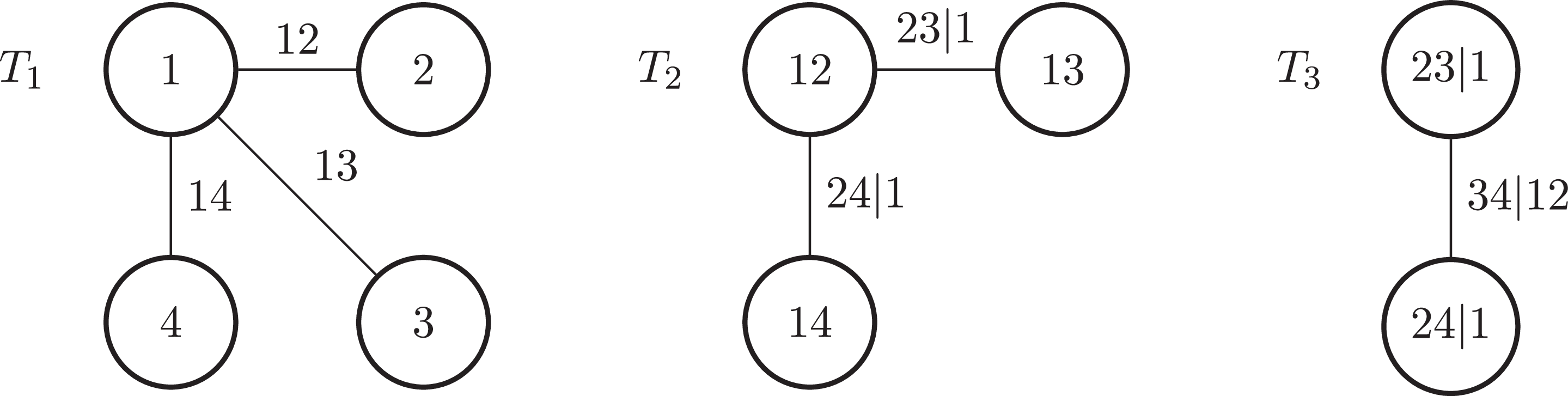
The formal definition may seem intimidating at first glance, so let us briefly consider an example with 4 variables, as shown in Figure 1. The key point is to understand how a vine helps us to understand what conditional constraints in higher-level trees are implied by our choices about the graph in lower-level trees.
A regular vine with four variables.

Looking at the graph of Figure 1 and applying equation (4):
 $$\eqalign{ & V = \left\{ {{T_1},\;{T_2},\;{T_3}} \right\} \cr & {T_1} = \left\{ {{N_1};{E_1}} \right\}\;\;\;\;\;\;\;\;\;\;\;\;\;\;\;\;{N_1} = \left\{ {1,2,3,4} \right\}\;\;\;\;\;\;\;\;\;\;\;\;\;\;{E_1} = \left\{ {\left( {1,2} \right),\left( {1,3} \right),\left( {1,4} \right)} \right\} \cr & {T_2} = \left\{ {{N_2};{E_2}} \right\}\;\;\;\;\;\;\;\;\;\;\;\;\;\;\;\;{N_2} = {E_1}\;\;\;\;\;\;\;\;\;\;\;\;\;\;\;\;\;\;\;\;\;\;\;\;\;{E_2} = \left\{ {\left( {\left( {1,2} \right),\left( {1,3} \right)} \right),\left( {\left( {1,2} \right),\left( {1,4} \right)} \right)} \right\} \cr & {T_3} = \left\{ {{N_3};{E_3}} \right\}\;\;\;\;\;\;\;\;\;\;\;\;\;\;\;\;{N_3} = {E_2}\;\;\;\;\;\;\;\;\;\;\;\;\;\;\;\;\;\;\;\;\;\;\;\;\;{E_3} = \left\{ {\left( {\left( {\left( {1,2} \right),\left( {1,3} \right)} \right),\left( {\left( {1,2} \right),\left( {1,4} \right)} \right)} \right)} \right\} \cr}$$
Tree
 ${{\bf{T}}_1}$
For the edges in
 ${E_1}$
we have the following:
 $${U_{\left( {1,2} \right)}} = \left\{ {1,2} \right\}$$
 $${U_{\left( {1,3} \right)}} = \left\{ {1,3} \right\}$$
 $${U_{\left( {1,4} \right)}} = \left\{ {1,4} \right\}$$
The edges in
 ${E_1}$
have empty conditioning sets and can be said to correspond to the pair copulas between variable
 ${X_1}$
and each of
 ${X_2}$
,
 ${X_3}$
and
 ${X_4}$
:
 $$\left( {1,2} \right) \,\longleftrightarrow \,{C_{12}}\left[ {{F_1}\left( {{x_1}} \right),{F_2}\left( {{x_2}} \right)} \right]$$
 $$\left( {1,3} \right) \,\longleftrightarrow \,{C_{13}}\left[ {{F_1}\left( {{x_1}} \right),{F_3}\left( {{x_3}} \right)} \right]$$
 $$\left( {1,4} \right) \,\longleftrightarrow\,{C_{14}}\left[ {{F_1}\left( {{x_1}} \right),{F_4}\left( {{x_4}} \right)} \right]$$
Tree
 ${{\bf{T}}_2}$
We must determine the constraint set, conditioning set and conditioned set for each edge
 $e \in {E_2}$
. With
 ${e_1} = ( {a,b}) = {\big( {( {1,2}), ( {1,3} )}\big)}$
we find:
 $${U_{{e_1}}} = {U_a} \cup {U_b} = \left\{ {1,2} \right\} \cup \left\{ {1,3} \right\} = \left\{ {1,2,3} \right\}$$
 $$\hskip -19pt{D_{{e_1}}} = {U_a} \cap {U_b} = \left\{ {1,2} \right\} \cap \left\{ {1,3} \right\} = \left\{ 1 \right\}$$
 $$\hskip -75pt\left\{ {{L_{{e_1},a}},{L_{{e_1},b}}} \right\} = \left\{ {{U_a}\backslash {D_{{e_1}}},{U_b}\backslash {D_{{e_1}}}} \right\} = \left\{ {2,3} \right\}$$
Taking
 ${{e_2} = \left( {a,c} \right) = \big( {( {1,2} ),( {1,4} )}\big)}$
we find:
 $${U_{{e_2}}} = {U_a} \cup {U_c} = \left\{ {1,2} \right\} \cup \left\{ {1,4} \right\} = \left\{ {1,2,4} \right\}$$
 $$\hskip -19pt{D_{{e_2}}} = {U_a} \cap {U_c} = \left\{ {1,2} \right\} \cap \left\{ {1,4} \right\} = \left\{ 1 \right\}$$
 $$\hskip -74.5pt\left\{ {{L_{{e_2},a}},{L_{{e_2},c}}} \right\} = \left\{ {{U_a}\backslash {D_{{e_2}}},{U_c}\backslash {D_{{e_2}}}} \right\} = \left\{ {2,4} \right\}$$
Therefore we can say that the elements of
 ${E_2}$
correspond to the pair copulas between
 ${X_2}$
and each of
 ${X_3}$
and
 ${X_4}$
, conditional on
 ${X_1}$
:
 $$\big( {( {1,2} ),( {1,3} )} \big) \,\longleftrightarrow\,{C_{23|1}}[{F_{2|1}}({x_2}|{x_1}),{F_{3|1}}({x_3}|{x_1})]$$
 $$\big( {( {1,2} ),( {1,4} )}\big ) \,\longleftrightarrow \,{C_{24|1}}[{F_{2|1}}({x_2}|{x_1}),{F_{4|1}}({x_4}|{x_1})]$$
Tree
 ${{\bf{T}}_3}$
 ${E_3}$
has a single element, so taking
 ${e_3} = \left( {{e_1},{e_2}} \right) = \left( {\left( {\left( {1,2} \right),\left( {1,3} \right)} \right),\left( {\left( {1,2} \right),\left( {1,4} \right)} \right)} \right)$
we find:
 $${U_{{e_3}}} = {U_{{e_1}}} \cup {U_{{e_2}}} = \left\{ {1,2,3} \right\} \cup \left\{ {1,2,4} \right\} = \left\{ {1,2,3,4} \right\}$$
 $$\hskip-19pt{D_{{e_3}}} = {U_{{e_1}}} \cap {U_{{e_2}}} = \left\{ {1,2,3} \right\} \cap \left\{ {1,2,4} \right\} = \left\{ {1,2} \right\}$$
 $$\hskip-108pt\left\{ {{L_{{e_3},{e_1}}},{L_{{e_3},{e_2}}}} \right\} = \left\{ {{U_{{e_1}}}\backslash {D_{{e_3}}},{U_{{e_2}}}\backslash {D_{{e_3}}}} \right\} = \left\{ {3,4} \right\}$$
We can say that the element of
 ${E_3}$
corresponds to the pair copula between
 ${X_3}$
and
 ${X_4}$
conditional on
 ${X_1}$
and
 ${X_2}$
:
 $$\big( {( {( {1,2} ),( {1,3} )} ),( {( {1,2} ),( {1,4} )} )} \big) \,\longleftrightarrow \,{C_{34|12}}[{F_{3|12}}({x_3}|{x_1},{x_2}),{F_{4|12}}({x_4}|{x_1},{x_2})]$$
3.4 Special cases
The general form given above for the regular vine gives rise to some commonly used special cases. This is primarily because the number of possible vine configurations grows very quickly as the number of dimensions increases. A vine is called canonical or a C-vine if each tree has a unique node to which all other nodes are connected. The example in Figure 1 is a C-vine. In this case with constraint set
 $D = \left\{ {1, \ldots, j - 1} \right\}$
the joint density can be written as the following product of the marginal densities and pair copula densities:
 $${f_{1 \ldots n}}\left( {{x_1},...,{x_n}} \right) = \mathop \prod \limits_{i = 1}^n {f_i}\left( {{x_i}} \right)\mathop \prod \limits_{j = 1}^{n - 1} \mathop \prod \limits_{k = 1}^{n - j} {c_{j,j + k|D}}[F({x_j}|{x_D}),F({x_{j + k}}|{x_D})]$$
A vine is called drawable or a D-vine if in each tree, all nodes are connected to at most two other nodes. With constraint set
 $D = \left\{ {k + 1, \ldots, k + j - 1} \right\}$
the corresponding joint density is then:
 $${f_{1 \ldots n}}\left( {{x_1},...,{x_n}} \right) = \mathop \prod \limits_{i = 1}^n {f_i}\left( {{x_i}} \right)\mathop \prod \limits_{j = 1}^{n - 1} \mathop \prod \limits_{k = 1}^{n - j} {c_{k,k + j|D}}[F({x_k}|{x_D}),F({x_{k + j}}|{x_D})]$$
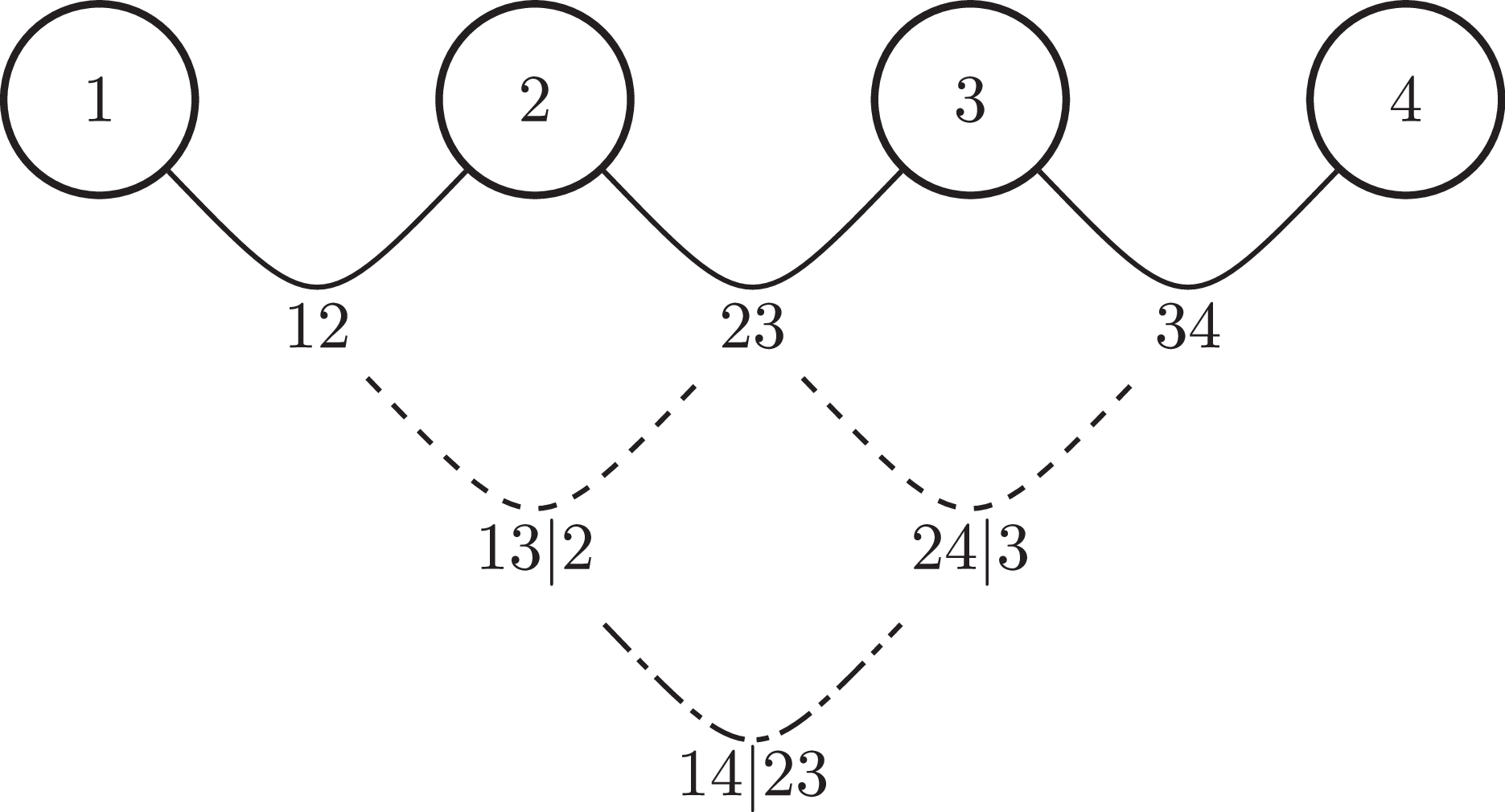
Figure 2 shows a 4-variable D-vine, using a slightly different representation, in which all trees are shown together and the edges in each higher order tree clearly join edges in the preceding tree. This differs from the representation in Figure 1 where each tree is drawn separately. D-vines can easily be drawn in either of these ways, which is where they get their name. For vines in general, however, it is easier to draw each tree separately as in Figure 1.
A drawable vine with four variables.

4. Vine-based approach for correlation between internal and external models
This section presents the main result of this paper. Having briefly introduced the notion of a vine copula, we now return to the modelling problem at hand. Recall our sets of pre-simulated data
 ${{\bf{X}}_A}$
and
 ${{\bf{X}}_B}$
. We wish to induce dependencies between the variables in these sets simply by re-ordering them relative to one another.
Define supplementary variable
 $Z$
with density
 $f\left( z \right)$
. By equation (3), we know that we can freely define one unconditional bivariate copula and
 $\left( {m - 1} \right)$
conditional bivariate copulas between
 $Z$
and
 ${X_i}{\rm{\;}},i \in A$
. Let
 ${c_{Z,i}}$
be the copula density between
 $Z$
and
 ${X_i}$
, then the joint density for
 $Z$
and
 ${{\bf{X}}_A}$
is:
 $${f_{AZ}}\left( {{x_1},...,{x_m},z} \right) = {f_Z}\left( z \right){f_A}\left( {{x_1},...,{x_m}} \right)\mathop \prod \limits_{i = 1}^m {c_{Z,i|1,,i - 1}}[F(z|{x_1},...,{x_{i - 1}}),F({x_i}|{x_1},...,{x_{i - 1}})]$$
This is equivalent to a C-vine schema where
 $Z$
is never the central node, and where we do not explicitly decompose the joint distribution of
 ${{\bf{X}}_A}$
into pair copulas, as this is the pre-simulated data whose distribution we wish to preserve. Similarly, we can define one unconditional and
 $\left( {n - m - 1} \right)$
conditional pair copulas between
 $Z$
and
 ${X_j}{\rm{\;}},j \in B$
. The joint density of
 $Z$
and
 ${{\bf{X}}_B}$
can therefore be written as:
 $$\eqalign {{f_{BZ}}\left( {{x_{m + 1}}, \ldots, {x_n},z} \right) & = {f_Z}\left( z \right){\rm{\;}}{f_B}\left( {{x_{m + 1}}, \ldots, {x_n}} \right) \cr & \times \mathop \prod \limits_{j = m + 1}^n {c_{Z,j|m + 1,...,j - 1}}[F(z|{x_{m + 1}},...,{x_{j - 1}}),F({x_j}|{x_{m + 1}},...,{x_{j - 1}})]}$$
This is a D-vine where
 $Z$
is always an end node, and where the joint distribution of
 ${{\bf{X}}_B}$
is not subjected to a pair copula decomposition. Omitting the variable arguments for brevity, and assuming conditional independence for all unspecified relations, the joint density for
 $Z$
,
 ${{\bf{X}}_A}$
and
 ${{\bf{X}}_B}$
is then:
 $${f_{ABZ}} = {f_Z}{\rm{\;}}{f_A}{\rm{\;}}{f_B}\mathop \prod \limits_{i = 1}^m {c_{Z,i|1, \ldots, i - 1}}\mathop \prod \limits_{j = m + 1}^n {c_{Z,j|m + 1, \ldots, j - 1}}$$
This is equivalent to a regular vine formed by joining some C-vine implicit in
 ${{\bf{X}}_A}$
to some D-vine implicit in
 ${{\bf{X}}_B}$
via a supplementary node
 $Z$
, such that
 ${X_i} \in {{\bf{X}}_A}$
and
 ${X_j} \in {{\bf{X}}_B}$
remain conditionally independent given
 $Z$
. The advantage of this formulation over the industry standard approach is that it allows us to specify, and achieve through sample re-ordering alone, more than one dependence relationship between variables in
 ${{\bf{X}}_A}$
and
 ${{\bf{X}}_B}$
, if we can specify these in terms of products of the form:
 $${c_{Z,i}} \cdot {c_{Z,j}}{\rm{\;\;\;\;\;\;\;\;}}i \in A,{\rm{\;}}j \in B$$
Products of this form are particularly tractable if all copulas are Gaussian, in which case they model
 ${\rho _{ij}} = {\rho _{zi}}{\rm{\;}}{\rho _{zj}}$
. We consider an example of this in Section 5.
4.1 Sampling algorithm
An example of an algorithm to sample from a joint density specified in this way is:
-
1. Define
${{\cal V}_A}$
as any C-vine including
$Z$
and
${{\bf{X}}_A} = \left\{ {{X_1},...,{X_m}} \right\}$
, where
$Z$
is never the central node (alternatively a D-vine where
$Z$
is always an end node).-
a. Only the choices of the pair copulas between
$Z$
and each
${X_i}$
are required, as we do not wish to alter the joint distribution of
${{\bf{X}}_A}$
. -
b. A vine structure for
${{\bf{X}}_A}$
can then be estimated, for instance using the approach of Dissmann et al. (Reference Dissmann, Brechmann, Czado and Kurowicka2013). -
c. The pair copulas for each edge can then be estimated, either parametrically, or non-parametrically using the approach of Nagler (Reference Nagler2018).
-
-
2. Take
${{\bf{X}}_A}$
as an observed sample from
${\cal V}_A^ - $
(the vine
${{\cal V}_A}$
excluding
$Z$
).-
a. Using the pair copula decomposition of
${{\bf{X}}_A}$
, find the random vector
${U_{{A^ - }}} = \left\{ {{U_1},...,{U_m}} \right\}$
where
${U_i} = F({X_i}|{X_1},...,{X_{i - 1}})$
using the Rosenblatt (Reference Rosenblatt1952) transformation. -
b. Draw
${U_Z}$
, a vector of observations from a standard uniform distribution, combine with
${U_{{A^ - }}}$
and let this equal
${U_A}$
. -
c. Using
${U_A}$
, sample a vector
${Z_A}$
from
${{\cal V}_A}$
, using for instance the algorithm of Aas et al. (Reference Aas, Czado, Frigessi and Bakken2009).
-
-
3. Define
${{\cal V}_B}$
as any D-vine including
$Z$
and
${{\bf{X}}_B}$
, where
$Z$
is always end node (or alternatively as any C-vine where
$Z$
is never the central node).-
a. Only the choices of the pair copulas between
$Z$
and each
${X_i}$
are required, as we do not wish to alter the joint distribution of
${{\bf{X}}_B}$
. -
b. A vine can be fitted to
${{\bf{X}}_B}$
as above. -
c. Take
${{\bf{X}}_B}$
as observed sample from
${\cal V}_B^ - $
(the vine
${{\cal V}_B}$
excluding
$Z$
), and determine -
•
${U_{{B^ - }}} = \left\{ {{U_{m + 1}},...,{U_n}} \right\}$
where
${U_i} = F({X_i}|{X_{m + 1}},...,{X_{i - 1}})$
. -
d. Combine
${U_Z}$
with
${U_{{B^ - }}}$
and let this equal
${U_B}$
. -
e. Using
${U_B}$
, sample vector
${Z_B}$
from
${{\cal V}_B}$
.
-
-
4. Re-order the ranks of
${Z_A}$
such that they equal the ranks of
${Z_B}$
. -
5. Re-order
${{\bf{X}}_A}$
to be consistent with
${Z_A}$
, and
${{\bf{X}}_B}$
to be consistent with
${Z_B}$
. -
6. Hence the joint sample has the joint density required.












In practical terms, correlation or rank correlation targets between the sets of pre-simulated data can then be achieved by the selection of the
 $Z$
-copulas, appropriately parameterised.
5. Example comparing industry standard and vine approaches
To demonstrate the proposed method and how it can be an improvement over the industry standard approach, this section sets out a low-dimensional example, in which all variables are Normally distributed and all copulas are Gaussian. Although an assumption of multivariate Normality is not very often used for modelling insurance risks or indeed market risk variables, I use it here as an exact solution is available. In the general case, numerical approaches must be taken.
Let
 ${{\bf{X}}_A} = \left( {{X_1},{X_2},{X_3}} \right)$
be a sample from our internal model, with trivariate Normal distribution, where the variables represent reserve risk, premium risk and catastrophe risk respectively, with correlation matrix:
 $${R_A} = \left( {\matrix{ {1 } & {{\rho _{12}}} & {{\rho _{13}}} \cr {0.67} & {1 } & {{\rho _{23}}} \cr {0.25} & {0.50} & {1 } \cr } } \right)$$
and let
 ${{\bf{X}}_B} = \left( {{X_4},{X_5},{X_6}} \right)$
be a sample from an external ESG, again with trivariate Normal distribution, where the variables represent equity risk, interest rate and inflation rate respectively, with correlation matrix:
 $${R_B} = \left( {\matrix{ {1 } & {{\rho _{45}}} & {{\rho _{46}}} \cr {0.30} & {1 } & {{\rho _{56}}} \cr {0.15} & {0.30} & {1 } \cr } } \right)$$
Note that, in each case, the variables within the internal model and the external model have positive correlations with each other.
Say we believe that our insurance risk results are likely to be worse when the economy is performing badly. This is a common assumption for insurers writing certain financial lines of business, for example, where periods of economic stress can result in reserve deterioration. To model this, we therefore choose to associate “bad” (low) values of the equity index variable
 ${X_4}$
with “bad” (high) values of reserve risk variable
 ${X_1}$
. One way for us to do this is by assuming these variables are negatively correlated somehow. For the sake of the example in this paper we will target a correlation of
 $ - 50{\rm{\% }}$
between
 ${X_1}$
and
 ${X_4}$
. Recall that the “catch,” as it were, is that we can only achieve this dependence by re-ordering the rows in the two samples relative to one another, while maintaining the joint structure within each sample.
5.1 Industry standard approach
Let copula
 ${C_{14}}$
be a bivariate Gaussian copula with correlation
 ${\rho _{14}} = - 50{\rm{\% }}$
between
 ${X_1}$
and
 ${X_4}$
. Because
 ${C_{14}}$
is Gaussian, the resulting joint distribution for all the variables is multivariate Normal.
Assuming conditional independence, the joint density can be written as:
 $${f_{AB}}\left( {{x_1},...,{x_6}} \right) = {f_A}\left( {{x_1},{x_2},{x_3}} \right){\rm{\;}}{f_B}\left( {{x_4},{x_5},{x_6}} \right){\rm{\;}}{c_{14}}\left[ {{F_1}\left( {{x_1}} \right),{F_4}\left( {{x_4}} \right)} \right]$$
We can use equation (2) to find the unspecified entries to complete the
 $6 \times 6$
correlation matrix:
 $${R_{AB}} = \left( {\matrix{ {{R_A}} & Y \cr {{Y^T}} & {{R_B}} \cr } } \right) = \left( {\matrix{ {1 } & {{\rho _{12}} } & {{\rho _{13}} } & {{\rho _{14}} } & {{\rho _{14}}{\rho _{45}} } & {{\rho _{14}}{\rho _{46}} } \cr {0.67 } & {1 } & {{\rho _{23}} } & {{\rho _{12}}{\rho _{14}} } & {{\rho _{12}}{\rho _{14}}{\rho _{45}} } & {{\rho _{12}}{\rho _{14}}{\rho _{46}} } \cr {0.25 } & {0.50 } & {1 } & {{\rho _{13}}{\rho _{14}} } & {{\rho _{13}}{\rho _{14}}{\rho _{45}} } & {{\rho _{13}}{\rho _{14}}{\rho _{46}} } \cr { - 0.50 } & { - 0.34 } & { - 0.13 } & {1 } & {{\rho _{45}} } & {{\rho _{46}} } \cr { - 0.15 } & { - 0.10 } & { - 0.04 } & {0.30 } & {1 } & {{\rho _{56}} } \cr { - 0.08 } & { - 0.05 } & { - 0.15 } & {0.15 } & {0.30 } & {1 } \cr } } \right)$$
and see that the selection of
 ${\rho _{14}}$
determines all of the resulting correlations between the other variables in
 ${{\bf{X}}_A}$
and
 ${{\bf{X}}_B}$
. So while we have achieved the target of
 $ - 50{\rm{\% }}$
between
 ${X_1}$
and
 ${X_4}$
we also have negative correlations for every other inter-model pair.
In particular each of the correlations between the insurance risks and inflation
 $\left\{ {{\rho _{16}},{\rho _{26}},{\rho _{36}}} \right\}$
are now also negative. This means we have associated low (good) values of inflation with high (bad) values of insurance risk. This is an unintended and undesirable outcome, as we typically expect high inflation to contribute to worse insurance risk outcomes, not the other way around. However, as we only have a single parameter, we cannot do anything about this.
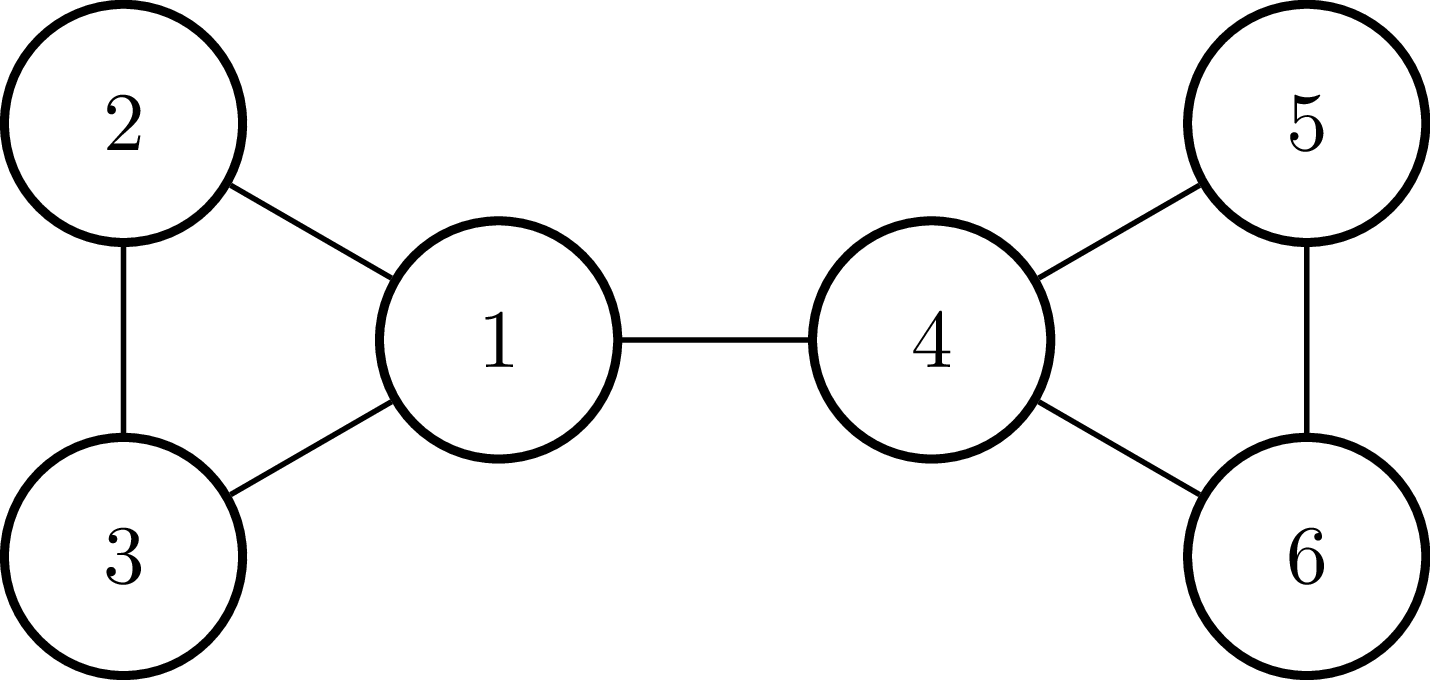
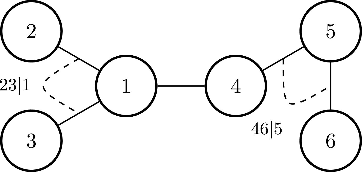
Another way to conceptualise the problem is to consider Figure 3, the adjacency graph of
 ${R_{AB}}$
excluding the diagonal and all conditionally independent relationships. Simply put, we would like to be able to add additional edges to this graph to control the extra dependencies we desire. However, we have the additional requirement that we can only achieve our targets by re-ordering the samples, so although there are methods to add further edges to the adjacency graph and determine the range of values that result in a valid correlation matrix, we lack a sampling algorithm.
Adjacency graph of
 ${R_{AB}}$
.

As we now see, the vine method allows us to achieve our aim, not only by allowing us to easily find valid parameterisations, but also because the sample algorithm relies only on re-ordering.
5.2 Vine copula method
Using a pair copula decomposition for the joint distribution, we can rewrite equation (6) in the following (non-unique) way, omitting arguments:
 $$\eqalign{ & {f_{AB}} = {f_A}\;{f_B}\;{c_{14}} \cr & \,\;\;\;\ = \left[ {{f_1}\;{f_2}\;{f_3}\;{c_{12}}\;{c_{13}}\;{c_{23|1}}\left] \times \right[{f_4}\;{f_5}\;{f_6}\;{c_{45}}\;{c_{56}}\;{c_{46|5}}} \right] \times {c_{14}} \cr & \ \ \ \ = {c_{12}}\;{c_{13}}\;{c_{14}}\;{c_{45}}\;{c_{56}}\;{c_{23|1}}\;{c_{46|5}}\prod\limits_{i = 1}^6 {{f_i}} \cr} $$
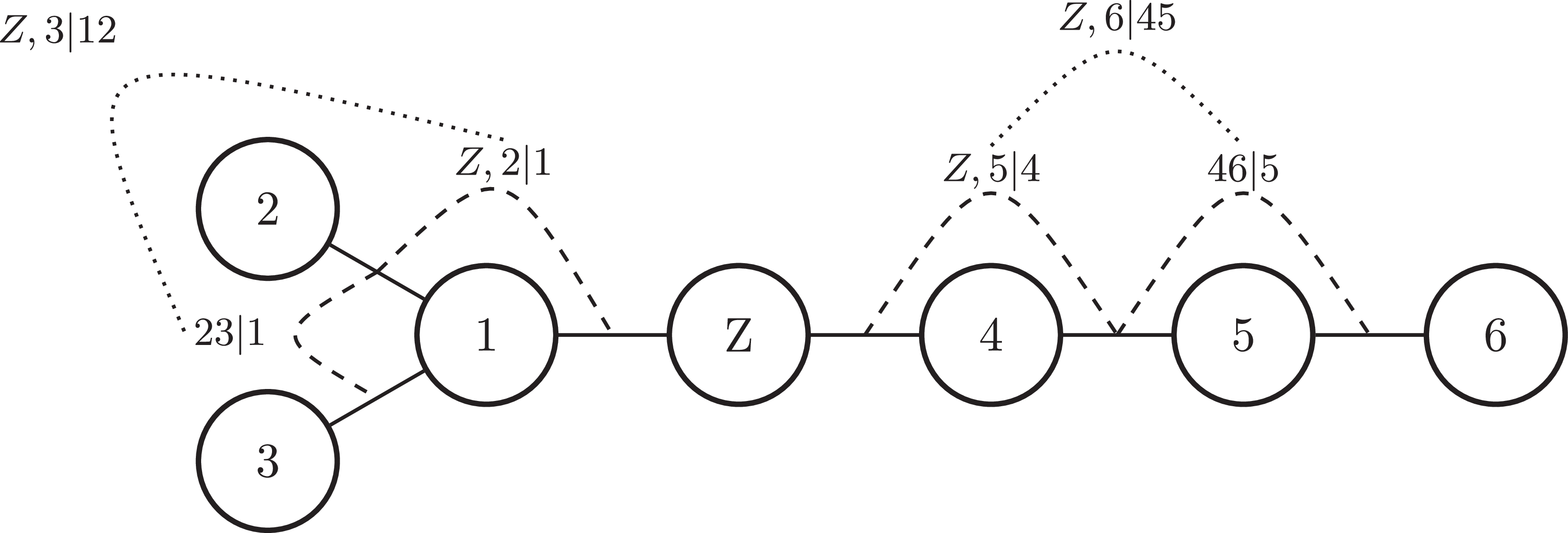
This factorisation of the joint density is expressed as a vine in Figure 4, where the nodes represent variables, solid edges between nodes represent the unconditional Gaussian pair copulas and dashed lines represent the conditional pair copulas
 ${C_{23|1}}$
and
 ${C_{46|5}}$
, which are implicit in
 ${{\bf{X}}_A}$
and
 ${{\bf{X}}_B}$
respectively. The similarities with Figure 3 are clear.
Vine copula on
 ${R_{AB}}$
.

Because
 ${{\bf{X}}_A}$
and
 ${{\bf{X}}_B}$
are Normally distributed, we have the nice property that the conditional copulas are also Gaussian, with conditional correlations
 ${\rho _{23|1}}$
and
 ${\rho _{46|5}}$
. Further, for any bivariate distribution with linear regression, the partial and conditional correlations are equal (Kurowicka & Cooke, Reference Kurowicka and Cooke2000). As the Normal distribution has this property, from the definition of partial correlation
 ${\rho _{ij;k}}$
we have the following relationship:
 $${\rho _{ij|k}} = {\rho _{ij;k}} = {{{\rho _{ij}} - {\rho _{ik}}{\rho _{jk}}} \over {\sqrt {1 - \rho _{ik}^2} \sqrt {1 - \rho _{jk}^2} }}$$
This gives us a convenient way to convert between the conditional correlations that parameterise the conditional copulas and the entries of the correlation matrix. As we can now associate a partial correlation with each edge in the vine, this is a so-called partial correlation vine.
Recall from equation (7) that when using the industry standard approach to model the desired negative correlation between reserve risk and equity market index, we necessarily ended up with unwanted negative correlations between the inflation rate and each of the insurance risks. We can now apply our main result from equation (5) by including our supplementary variable
 $Z$
to avoid this outcome.
Let the joint density of
 ${{\bf{X}}_A}$
,
 ${{\bf{X}}_B}$
and
 $Z$
be:
 $${f_{ABZ}}\left( {{x_1}, \ldots, {x_6},z} \right) = {f_A}{\rm{\;}}{f_B}{\rm{\;}}{f_Z}{\rm{\;}}{c_{Z,1}}{\rm{\;}}{c_{Z,2|1}}{\rm{\;}}{c_{Z,3|12}}{\rm{\;}}{c_{Z,4}}{\rm{\;}}{c_{Z,5|4}}{\rm{\;}}{c_{Z,6|45}}$$
where all of the copula densities involving
 $Z$
are Gaussian. Therefore the joint distribution for all variables is Normal with correlation matrix:
 $${R_{ABZ}} = \left( {\matrix{ {{R_A}} & {{Z_A}} & Y \cr {Z_A^T} & {1 } & {Z_B^T} \cr {{Y^T}} & {{Z_B}} & {{R_B}} \cr } } \right){\rm{\;\;\;\;\;\;\;\;where}}:{\rm{\;\;\;\;}}{Z_A} = \left( {\matrix{ {{\rho _{Z,1}}} \cr {{\rho _{Z,2}}} \cr {{\rho _{Z,3}}} \cr } } \right){\rm{\;\;\;\;and\;\;\;\;}}{Z_B} = \left( {\matrix{ {{\rho _{Z,4}}} \cr {{\rho _{Z,5}}} \cr {{\rho _{Z,6}}} \cr } } \right)$$
To find the entries of
 ${Z_A}$
and
 ${Z_B}$
, we can recursively apply equation (9) to find the correlation between the specified pairs given the parameters for the copulas in the vine. For example:
 $${\rho _{Z,2}} = {\rho _{Z,2|1}}\sqrt {1 - \rho _{12}^2} \sqrt {1 - \rho _{Z,1}^2} + {\rho _{12}}{\rm{\;}}{\rho _{Z,1}}$$
To find entries of
 $Y$
, recall that all
 $\left\{ {{X_i},{X_j}} \right\},{\rm{\;\;}}i \in A,{\rm{\;\;}}j \in B$
are conditionally independent, that is,
 ${\rho _{ij|Z}} = 0$
. Hence, we find:
 $$Y = {Z_A}Z_B^T = \left( {\matrix{ {{\rho _{Z,1}}{\rho _{Z,4}}} \hfill & {{\rho _{Z,1}}{\rho _{Z,5}}} \hfill & {{\rho _{Z,1}}{\rho _{Z,6}}} \hfill \cr {{\rho _{Z,2}}{\rho _{Z,4}}} \hfill & {{\rho _{Z,2}}{\rho _{Z,5}}} \hfill & {{\rho _{Z,2}}{\rho _{Z,6}}} \hfill \cr {{\rho _{Z,3}}{\rho _{Z,4}}} \hfill & {{\rho _{Z,3}}{\rho _{Z,5}}} \hfill & {{\rho _{Z,3}}{\rho _{Z,6}}} \hfill \cr } } \right)$$
Compare this result to the industry standard approach. We now have six parameters to control the inter-model correlations and can specify more than one target. To resolve the issue of negative correlation between inflation and insurance risks, we specify that the correlations between each insurance risk and inflation should be no less than
 $5{\rm{\% }}$
. We therefore have the following requirements:
 $$\eqalign{{{\rho _{14}} = {\rho _{Z,1}} {\rho _{Z,4}} = - 0.5}\hskip2pc} \\ \,{\rho _{i6}} = {\rho _{Z,i}}{\rho _{Z,6}} \ge 0.05{\rm{\;\;}},i \in \left\{ {1,2,3} \right\}$$
This leaves us with several unspecified entries in
 $Y$
. To find a unique solution we therefore include another requirement: that we seek the solution which introduces the minimum amount of extra information beyond our specified targets. For the Normal distribution this is equivalent to maximising the determinant of the correlation matrix (Whittaker, Reference Whittaker2009), which corresponds to maximising entropy.
We parameterise the vine copula by vector
 ${\theta ^T} = \left( {{\rho _{Z,1}},{\rho _{Z,2|1}},{\rho _{Z,3|12}},{\rho _{Z,4}},{\rho _{Z,5|4}},{\rho _{Z,6|54}}} \right)$
where each element represents the (un)conditional correlation linking
 $Z$
to the respective
 ${X_i}$
. Clearly each value is bounded in the range
 $\left[ { - 1,1} \right]$
. Subject to our constraints in equation (11), the optimal parameter vector
 ${\theta ^{\rm{*}}}$
is found by solving the following optimisation problem:
 $${\theta ^{\rm{*}}} = {\rm{arg}}\mathop {\max }\limits_\theta {\rm{det}}\ {R_{ABZ}}$$
Although maximising the determinant of
 ${R_{ABZ}}$
directly is possible, we can leverage the partial correlation vine structure for
 ${R_{AB}}$
from equation (8) to rewrite equation (10) as a partial correlation vine for
 ${R_{ABZ}}$
, as shown in Figure 5. From Kurowicka and Cooke (Reference Kurowicka and Cooke2006) we have that the determinant
 $D$
of an
 $n$
-dimensional correlation matrix
 $R$
can be expressed as the following product of terms involving the partial correlations and edges from
 ${\cal V}$
, a partial correlation vine on
 $R$
:
 $$D = \mathop \prod \limits_{e \in E\left( {\cal V} \right)} {(1 - {\rho _{{e_1},{e_2};{D_e}}})^2}$$
Vine copula on
 $R_{ABZ}$
.

The clear benefit of this approach is that we can simplify the optimisation problem by setting to zero the partial correlation for any edges in the graph where we have assumed conditional independence. We find the following solution for
 ${\theta ^{\rm{*}}}$
and
 ${Y^{\rm{*}}}$
, the matrix of achieved inter-model correlations:
 $${\theta ^{\rm{*}}} = \left( {\matrix{ {0.72} \hfill \cr {0.08} \hfill \cr {0.18} \hfill \cr { - 0.69} \hfill \cr {0.10} \hfill \cr {0.36} \hfill \cr } } \right)\ \ \ \ \ \ \ \ {Y^{\rm{*}}} = \left( {\matrix{ { - 0.50} \hfill & { - 0.10} \hfill & {0.11} \hfill \cr { - 0.36} \hfill & { - 0.07} \hfill & {0.08} \hfill \cr { - 0.21} \hfill & { - 0.04} \hfill & {0.05} \hfill \cr } } \right)$$
We can now see that in addition to achieving the target correlation of
 $ - 50{\rm{\% }}$
between reserve risk
 ${X_1}$
and equity index
 ${X_4}$
, using the vine copula approach we can also achieve our additional targets, of at least
 $5{\rm{\% }}$
correlation between each of reserve risk
 ${X_1}$
, premium risk
 ${X_2}$
, catastrophe risk
 ${X_3}$
and inflation rate
 ${X_6}$
.
Given
 ${\theta ^{\rm{*}}}$
and pre-simulated samples
 ${{\bf{X}}_A}$
,
 ${{\bf{X}}_B}$
, one can now produce a sample from the joint distribution that has the inter-model correlations
 ${Y^{\rm{*}}}$
, using the algorithm described earlier.
6. Conclusion
This paper describes a problem often faced in capital modelling–that of specifying and achieving dependencies between internal and external models–and provides a method that goes some way to addressing the limitations of the industry standard approach.
It does this by allowing for the specification of more than one dependence relationship between sets of pre-simulated data, which can be used either to achieve more than one target correlation between pairs; or just to control for unintended and unwanted side-effects of targeting a specific important correlation.
 RAB
 RAB
 RABZ

 Open access

