1 Introduction
The motivation for our present work is the following simple experiment. Starting with a uniformly mixed suspension of negatively buoyant particles (
 $\unicode[STIX]{x1D70C}_{p}>\unicode[STIX]{x1D70C}_{\ell }$
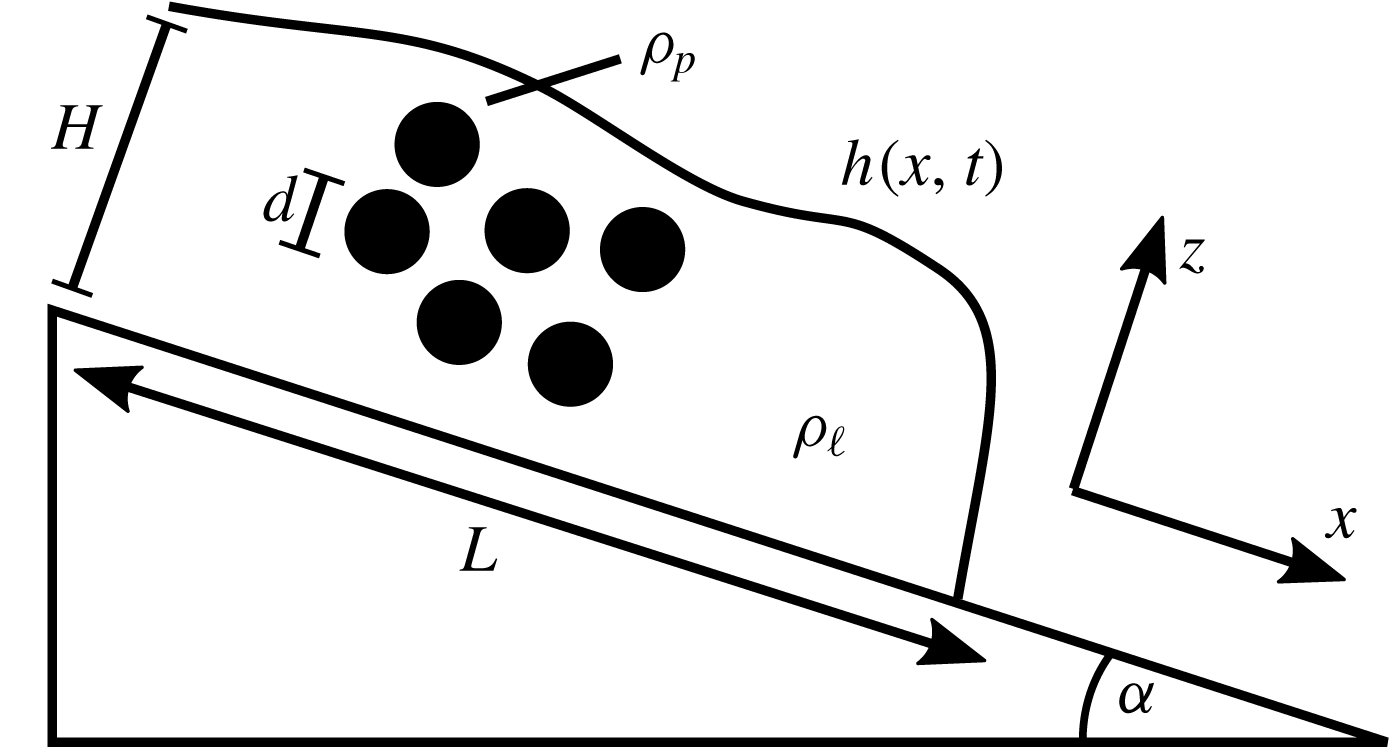
) in a viscous fluid, a volume of this mixture is poured into a wide, inclined channel and allowed to flow under the influence of gravity (see figure 1). We consider introducing either a finite initial volume or a constant flux of a mixed suspension at the top of the incline. The particles are uniform spheres of diameter
 $d$
, large enough that shear-induced migration (rather than Brownian diffusion) drives the particle motion relative to the fluid. The film has a characteristic height
 $H$
and an
 $x$
-scale
 $L$
satisfying
 $$\begin{eqnarray}\frac{H}{L}\ll \left(\frac{d}{H}\right)^{2}\ll 1,\end{eqnarray}$$
which is the asymptotic regime in which the film is thin (the lubrication limit) and the migration of particles in the normal direction is fast relative to the flow down the incline.
Problem diagram. A suspension with particle and fluid densities
 $\unicode[STIX]{x1D70C}_{p}$
and
 $\unicode[STIX]{x1D70C}_{\ell }$
with a free surface
 $h(x,t)$
and
 $\unicode[STIX]{x1D70C}_{p}>\unicode[STIX]{x1D70C}_{\ell }$
flows under the influence of gravity down an incline at an angle
 $\unicode[STIX]{x1D6FC}$
from horizontal. The film has a characteristic height
 $H$
and length
 $L$
with
 $H\ll L$
.

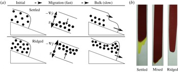
(a) Evolution of the flow on two different time scales. On the fast time scale, particles migrate in
 $z$
due to settling (
 $g$
) and shear-induced migration (
 $\dot{\unicode[STIX]{x1D6FE}}$
is the shear rate). On the slow time scale, the particles are in
 $z$
-equilibrium, either settling to the substrate or accumulating at the surface. (b) Images of each regime from experiments done at UCLA Fluids Lab; the centre image shows the ‘mixed’ regime where the equilibrium distribution is nearly uniform.

Under this assumption, there are two phases to the development of the flow from a uniform mixture (Murisic et al.
Reference Murisic, Ho, Hu, Latterman, Koch, Lin, Mata and Bertozzi2011, Reference Murisic, Pausader, Peschka and Bertozzi2013). Initially, the particles rapidly equilibrate in the normal direction. In the ‘settled regime’, particles settle to the substrate, leaving a clear fluid layer above; in the ‘ridged regime’, they accumulate towards the free surface (see figure 2). This determines the suspension velocity profile, which can be depth-integrated in the lubrication limit to produce a pair of hyperbolic conservation laws depending only on
 $x$
and
 $t$
(time) for the film height and depth-averaged particle concentration. The behaviour of this bulk flow is determined by the equilibrium concentration profile. As shown experimentally (Zhou et al.
Reference Zhou, Dupuy, Bertozzi and Hosoi2005; Ward et al.
Reference Ward, Wey, Glidden, Hosoi and Bertozzi2009; Murisic et al.
Reference Murisic, Ho, Hu, Latterman, Koch, Lin, Mata and Bertozzi2011) and theoretically (Murisic et al.
Reference Murisic, Ho, Hu, Latterman, Koch, Lin, Mata and Bertozzi2011, Reference Murisic, Pausader, Peschka and Bertozzi2013), below a ‘critical concentration’
 $\unicode[STIX]{x1D719}_{c}$
the suspension is in the settled regime and the particle and fluid phases tend to separate, producing two advancing fronts with pure fluid flowing ahead of the particles. Above the critical concentration is the ridged regime, where the particles accumulate at a single particle-rich front. Exactly at the critical concentration, the suspension remains uniformly mixed. Such models that assume a rapid equilibration in the normal direction to the bulk flow have been used to study the properties of the bulk flow such as the evolution of the particle and fluid fronts (Murisic et al.
Reference Murisic, Pausader, Peschka and Bertozzi2013; Wang & Bertozzi Reference Wang and Bertozzi2014), shock and singular shock solutions (Cook, Bertozzi & Hosoi Reference Cook, Bertozzi and Hosoi2008; Wang & Bertozzi Reference Wang and Bertozzi2014) and flow in helical channels (Lee, Stokes & Bertozzi Reference Lee, Stokes and Bertozzi2014; Arnold, Stokes & Green Reference Arnold, Stokes and Green2015).
More broadly, our work fits into the study of particle-laden flows (see Delannay et al. (Reference Delannay, Valance, Mangeney and Richard2017) for a review), which includes the study of landslides (Katz & Aharonov Reference Katz and Aharonov2006; Leonardi Reference Leonardi2015) and more fundamental engineering questions on using oil-contaminated sand for construction (Abousnina et al. Reference Abousnina, Manalo, Shiau and Lokuge2015). There are also many industrial applications that arise including how particle-laden fluids drain (Chen, Malambri & Lee Reference Chen, Malambri and Lee2018) and the behaviour of processed foods (Lareo, Fryer & Barigou Reference Lareo, Fryer and Barigou1997) – including molten chocolate as it is being prepared (Taylor et al. Reference Taylor, Van Damme, Johns, Routh and Wilson2009). The phenomenon of shear-induced migration has been a subject of considerable interest; prior work on the incline problem, notably that of Murisic et al. (Reference Murisic, Pausader, Peschka and Bertozzi2013), utilized the diffusive flux model of Leighton & Acrivos (Reference Leighton and Acrivos1987). Here we employ a simplified suspension balance model instead in which the migration is modelled through a normal stress in the particle phase (Morris & Boulay Reference Morris and Boulay1999; Miller & Morris Reference Miller and Morris2006). This model has been employed to some success in studying shear-induced migration in Couette flow (Boyer, Pouliquen & Guazzelli Reference Boyer, Pouliquen and Guazzelli2011), steady flow of a free surface film on an incline (Timberlake & Morris Reference Timberlake and Morris2005) and secondary flows in inclined channels (Ramachandran & Leighton Reference Ramachandran and Leighton2008), despite some potential inconsistencies (Nott, Guazzelli & Pouliquen Reference Nott, Guazzelli and Pouliquen2011).
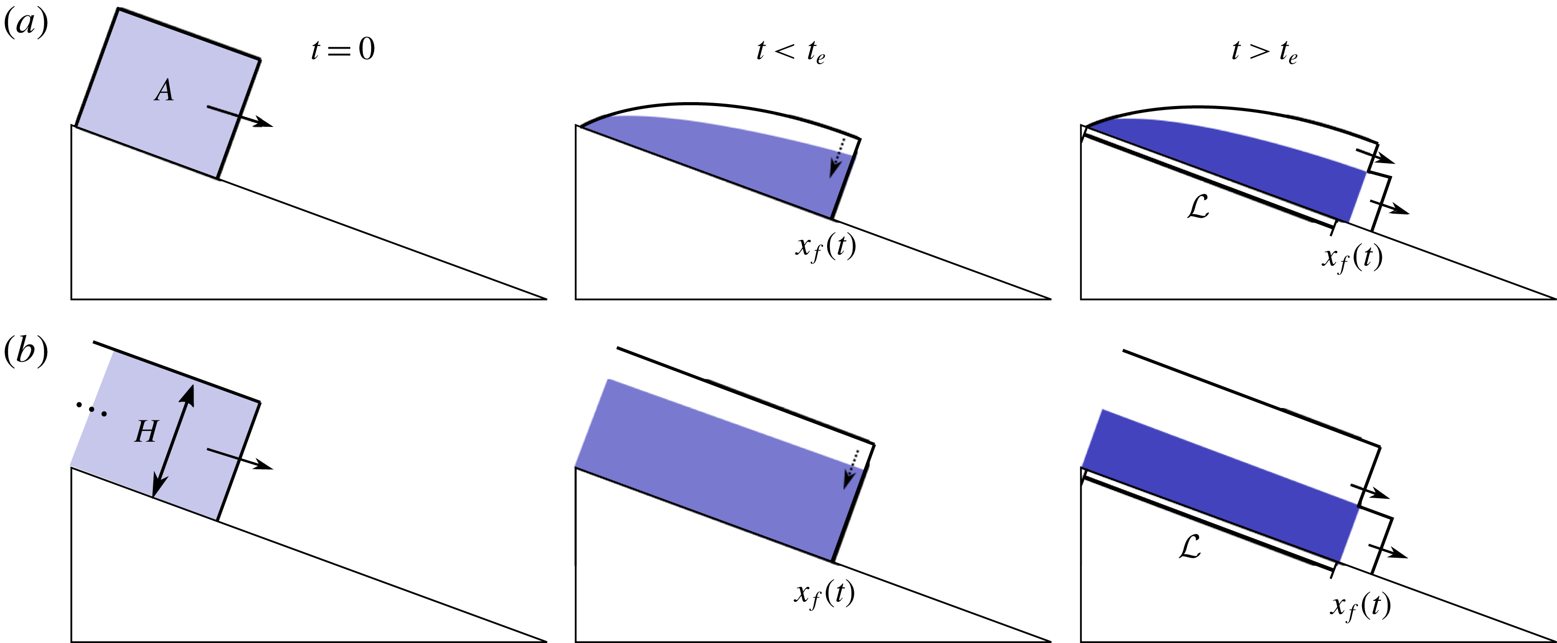
In the settled regime, sketch of the model for the ‘transition distance’
 ${\mathcal{L}}$
before the suspension separates into distinct fronts, given either a fixed initial area
 $A$
(a) or constant upstream height
 $H$
(b). The bulk flow is assumed to evolve as well-mixed up to a time
 $t_{e}$
as the particles equilibrate in the
 $z$
-direction.

While the bulk flow model yields accurate predictions, it is only appropriate once the particles have reached
 $z$
-equilibrium (see figure 1 for the coordinate system). In this paper, our primary focus is understanding this equilibration process and how it relates to the properties of the flow. Notably, we endeavour to obtain a simple estimate for the length and time scales over which the suspension establishes either a settled or ridged behaviour. Figure 3 illustrates our heuristic: the suspension begins well-mixed, either with a finite initial volume or with a constant volumetric flux; as equilibrium is established in the
 $z$
-direction, we approximate the bulk fluid flow as though it is well-mixed; and once equilibrium is established, the suspension flows in either the settled or ridged regime.
On the time scale for equilibration, the model reduces to a degenerate nonlinear diffusion equation for the particles in the
 $z$
-direction driven by the shear flow (§ 2), similar to the equation describing Taylor dispersion (Taylor Reference Taylor1954). Degenerate parabolic equations with similar structure arise in the study of sedimenting particles in a quiescent fluid (Berres, Bürger & Tory Reference Berres, Bürger and Tory2005). The solutions to our model equations converge to the equilibrium profile assumed in models for bulk incline flow. Through analysis of the fast diffusion equation (§ 3) we estimate the time required for equilibration, and in § 4 we compare to experiments in prior work by Murisic et al. (Reference Murisic, Ho, Hu, Latterman, Koch, Lin, Mata and Bertozzi2011). In that work, it was speculated that for an initially uniform suspension, the time scale for
 $z$
-equilibration diverges as the mixture approaches the critical concentration, from experimental observations (e.g. the mixed regime in figure 2) where the mixture travels a long distance before separating. We address this claim and show that the mathematical model exhibits this divergence in the settled regime. Finally, we consider the ridged regime and the behaviour of the model at high concentrations in appendix B.
2 Particle equilibration model
Consider, as depicted in figure 1, an inclined plane at an angle
 $\unicode[STIX]{x1D6FC}$
from horizontal with coordinates
 $x$
and
 $z$
aligned, respectively, down and normal to the incline. Adopting a simplified suspension balance model (Morris & Boulay Reference Morris and Boulay1999; Miller & Morris Reference Miller and Morris2006), we derive equations for the film height
 $h(x,t)$
, the particle concentration
 $\unicode[STIX]{x1D719}(x,z,t)$
and the depth-integrated concentration
 $$\begin{eqnarray}\overline{\unicode[STIX]{x1D719}}(x,t)=\frac{1}{h}\int _{0}^{h}\unicode[STIX]{x1D719}(x,z,t)\,\text{d}z.\end{eqnarray}$$
The depth-integrated equations become a pair of equations for
 $h$
and
 $\overline{\unicode[STIX]{x1D719}}$
, with fluxes determined by the equilibrium distribution of particles (Murisic et al.
Reference Murisic, Pausader, Peschka and Bertozzi2013). This equilibrium model framework has provided an understanding of the bulk flow properties after
 $z$
-equilibrium has been established.
The starting point for our work is to introduce a fast time scale on which the system reaches its
 $z$
-equilibrium distribution. Within this framework, we uncover a nonlinear diffusion process that governs the particle dynamics. Analysis of the resulting equations allows us to make predictions relevant to experiments studying the bulk flow.
2.1 Review of suspension balance model
First, we state the model equations for the time-dependent incline flow, leaving the time scale unspecified. The derivation here follows Miller & Morris (Reference Miller and Morris2006) and extends that by Timberlake & Morris (Reference Timberlake and Morris2005), wherein the equations are derived for steady flow. Let
 $\boldsymbol{u}=(u,w)$
be the suspension velocity and let
 $\unicode[STIX]{x1D70C}(\unicode[STIX]{x1D719})$
be the effective density, given by
 $$\begin{eqnarray}\unicode[STIX]{x1D70C}(\unicode[STIX]{x1D719})/\unicode[STIX]{x1D70C}_{\ell }=1+b\unicode[STIX]{x1D719},\quad b:=\unicode[STIX]{x1D70C}_{p}/\unicode[STIX]{x1D70C}_{\ell }-1.\end{eqnarray}$$
We assume for our work that
 $b>0$
, i.e. the particles are denser than the fluid (but the derivation we present is valid for neutrally and positively buoyant particles, too). The model equations consist of incompressibility and momentum balance for the suspension and a particle transport equation:
 $$\begin{eqnarray}\displaystyle & \displaystyle 0=\unicode[STIX]{x1D735}\boldsymbol{\cdot }\boldsymbol{u}, & \displaystyle\end{eqnarray}$$
 $$\begin{eqnarray}\displaystyle & \displaystyle \unicode[STIX]{x1D70C}\frac{\text{D}u}{\text{D}t}=-\unicode[STIX]{x1D735}p+\unicode[STIX]{x1D735}\boldsymbol{\cdot }\unicode[STIX]{x1D72E}_{s}+\unicode[STIX]{x1D70C}\boldsymbol{g}, & \displaystyle\end{eqnarray}$$
 $$\begin{eqnarray}\displaystyle & \displaystyle \frac{\unicode[STIX]{x2202}\unicode[STIX]{x1D719}}{\unicode[STIX]{x2202}t}+\boldsymbol{u}\boldsymbol{\cdot }\unicode[STIX]{x1D735}\unicode[STIX]{x1D719}=-\unicode[STIX]{x1D735}\boldsymbol{\cdot }\boldsymbol{J}, & \displaystyle\end{eqnarray}$$
 $\boldsymbol{J}$
is the particle flux relative to the suspension average,
 $\boldsymbol{g}=g(\sin \unicode[STIX]{x1D6FC},-\cos \unicode[STIX]{x1D6FC})$
and
 $g=9.8~\text{m}~\text{s}^{-2}$
. The suspension stress and particle phase stress (to be used in (2.8)) are
 $$\begin{eqnarray}\unicode[STIX]{x1D72E}_{s}=\unicode[STIX]{x1D707}^{(s)}(\unicode[STIX]{x1D719})\unicode[STIX]{x1D640}+\unicode[STIX]{x1D72E}_{N},\quad \unicode[STIX]{x1D72E}_{p}=(\unicode[STIX]{x1D707}^{(s)}(\unicode[STIX]{x1D719})-\unicode[STIX]{x1D707}_{\ell })\unicode[STIX]{x1D640}+\unicode[STIX]{x1D72E}_{N},\end{eqnarray}$$
where
 $\unicode[STIX]{x1D640}=\frac{1}{2}(\unicode[STIX]{x1D735}\boldsymbol{u}+\unicode[STIX]{x1D735}\boldsymbol{u}^{\text{T}})$
,
 $\unicode[STIX]{x1D707}^{(s)}(\unicode[STIX]{x1D719})$
is the suspension viscosity and the Reynolds stress contribution to the suspension stress has been neglected. As in Miller & Morris (Reference Miller and Morris2006), the expression for the normal stress in the lubrication limit is taken to be
 $$\begin{eqnarray}\unicode[STIX]{x1D72E}_{N}=-\unicode[STIX]{x1D707}^{(n)}(\unicode[STIX]{x1D719})\dot{\unicode[STIX]{x1D6FE}}(\unicode[STIX]{x1D6EC}_{1}\boldsymbol{e}_{x}\boldsymbol{e}_{x}^{\text{T}}+\unicode[STIX]{x1D6EC}_{2}\boldsymbol{e}_{z}\boldsymbol{e}_{z}^{\text{T}}),\end{eqnarray}$$
where
 $\boldsymbol{e}_{x}$
and
 $\boldsymbol{e}_{z}$
are unit column vectors in the
 $x$
and
 $z$
directions,
 $\dot{\unicode[STIX]{x1D6FE}}=\sqrt{2\unicode[STIX]{x1D640}\boldsymbol{ :}\unicode[STIX]{x1D640}}$
is the shear rate,
 $\unicode[STIX]{x1D6EC}_{1}=1$
and
 $\unicode[STIX]{x1D6EC}_{2}=0.8$
. The principal stress is aligned with the flow (
 $x$
) and gradient (
 $z$
) directions. Note that this stress is proportional to the shear rate, which is
 $\dot{\unicode[STIX]{x1D6FE}}\approx |u_{z}|$
for a thin film. We use the normal and suspension viscosities
 $\unicode[STIX]{x1D707}^{(n)},\unicode[STIX]{x1D707}^{(s)}$
from (Boyer et al.
Reference Boyer, Pouliquen and Guazzelli2011) and scaled versions
 $\hat{\unicode[STIX]{x1D707}}^{(n)},\hat{\unicode[STIX]{x1D707}}^{(s)}$
given by
 $$\begin{eqnarray}\displaystyle & \displaystyle \frac{\unicode[STIX]{x1D707}^{(n)}(\unicode[STIX]{x1D719})}{K_{n}\unicode[STIX]{x1D707}_{\ell }}=\hat{\unicode[STIX]{x1D707}}^{(n)}:=\frac{(\unicode[STIX]{x1D719}/\unicode[STIX]{x1D719}_{m})^{2}}{(1-\unicode[STIX]{x1D719}/\unicode[STIX]{x1D719}_{m})^{2}}, & \displaystyle\end{eqnarray}$$
 $$\begin{eqnarray}\displaystyle & \displaystyle \frac{\unicode[STIX]{x1D707}^{(s)}(\unicode[STIX]{x1D719})}{\unicode[STIX]{x1D707}_{\ell }}=\hat{\unicode[STIX]{x1D707}}^{(s)}:=1+\frac{5}{2}\frac{\unicode[STIX]{x1D719}}{(1-\unicode[STIX]{x1D719}/\unicode[STIX]{x1D719}_{m})}+I(\unicode[STIX]{x1D719})\frac{(\unicode[STIX]{x1D719}/\unicode[STIX]{x1D719}_{m})^{2}}{\left(1-\unicode[STIX]{x1D719}/\unicode[STIX]{x1D719}_{m}\right)^{2}}. & \displaystyle\end{eqnarray}$$
 $\unicode[STIX]{x1D719}_{m}=0.58$
is the maximum packing fraction,
 $K_{n}$
is a normal viscosity coefficient and the function
 $I(\unicode[STIX]{x1D719})$
corrects for the behaviour at high concentrations and is given by
 $$\begin{eqnarray}I(\unicode[STIX]{x1D719})=m_{1}+(m_{2}-m_{1})/(1+I_{0}\unicode[STIX]{x1D719}^{2}/(\unicode[STIX]{x1D719}_{m}-\unicode[STIX]{x1D719})^{2}).\end{eqnarray}$$
The constants used here are
 $K_{n}=1,I_{0}=0.005,\,m_{1}=0.32$
and
 $m_{2}=0.7$
. The value of
 $K_{n}$
, which controls the balance between shear-induced migration and sedimentation, is chosen to best match the existing theory for particles in
 $z$
-equilibrium (as we discuss in § 2.3). While the coefficients such as
 $K_{n}$
may depend on concentration (Dbouk, Lobry & Lemaire Reference Dbouk, Lobry and Lemaire2013), we take it to be constant for simplicity. As in Miller & Morris (Reference Miller and Morris2006) we use the following expression for the particle flux in (2.3c
):
 $$\begin{eqnarray}\boldsymbol{J}=\frac{d^{2}}{18\unicode[STIX]{x1D707}_{\ell }}f_{h}(\unicode[STIX]{x1D719})(\unicode[STIX]{x1D735}\boldsymbol{\cdot }\unicode[STIX]{x1D72E}_{p}+\unicode[STIX]{x1D70C}_{\ell }b\unicode[STIX]{x1D719}\boldsymbol{g}).\end{eqnarray}$$
The first term is the contribution from the particle stress, and the second is due to sedimentation (note that the Stokes settling velocity is
 $(\unicode[STIX]{x1D70C}_{p}-\unicode[STIX]{x1D70C}_{\ell })d^{2}g/18\unicode[STIX]{x1D707}_{\ell }$
). The hindrance function
 $f_{h}(\unicode[STIX]{x1D719})$
accounts for the effect of the particle concentration on the Stokes drag force and is chosen to be
 $$\begin{eqnarray}f_{h}(\unicode[STIX]{x1D719})=(1-\unicode[STIX]{x1D719}/\unicode[STIX]{x1D719}_{m})(1-\unicode[STIX]{x1D719})^{2}.\end{eqnarray}$$
The reduction of the governing equations (2.3) in the lubrication limit is standard (Oron, Davis & Bankoff Reference Oron, Davis and Bankoff1997; Murisic et al. Reference Murisic, Pausader, Peschka and Bertozzi2013). Non-dimensional quantities (denoted with a hat) are defined as follows:
 $$\begin{eqnarray}\displaystyle (x,z)=L(\hat{x},\unicode[STIX]{x1D716}\hat{z}),\quad (u,w)=U(\hat{u} ,\unicode[STIX]{x1D716}{\hat{w}}),\quad t=T\hat{t},\quad p=p_{a}+\frac{\unicode[STIX]{x1D707}_{\ell }U}{H}\hat{p},\quad J=\frac{\text{d}^{2}U}{18H^{2}}{\hat{J}}, & & \displaystyle \nonumber\\ \displaystyle & & \displaystyle\end{eqnarray}$$
where
 $\unicode[STIX]{x1D716}=H/L$
, the atmospheric pressure is
 $p_{a}$
and
 $T$
is a time scale to be selected later. The value of
 $U$
is chosen to balance gravity and the suspension viscous stress, leading to
 $$\begin{eqnarray}U=\frac{H^{2}\unicode[STIX]{x1D70C}_{\ell }g\sin \unicode[STIX]{x1D6FC}}{\unicode[STIX]{x1D707}_{\ell }}.\end{eqnarray}$$
As discussed in the introduction, the equations are studied in the asymptotic limit
 $$\begin{eqnarray}\unicode[STIX]{x1D716}\ll \left(d/H\right)^{2}\ll 1,\end{eqnarray}$$
which ensures that the time scale for normal equilibration of particles is fast relative to the bulk flow (Murisic et al. Reference Murisic, Pausader, Peschka and Bertozzi2013). The non-dimensional shear rate is
 $$\begin{eqnarray}\hat{\unicode[STIX]{x1D6FE}}=\frac{H}{U}\dot{\unicode[STIX]{x1D6FE}}\approx |\hat{u} _{\hat{z}}|.\end{eqnarray}$$
Near the free surface, there is a non-local contribution to the shear rate (Miller & Morris Reference Miller and Morris2006) of size
 $O(d/H)$
. For simplicity, we elect to use (2.13) as the adjustment has little effect on solutions except at very high concentrations (addressed in appendix B).
Non-dimensionalizing the suspension balance equations (2.3), substituting in the expression (2.5) for the normal stress and retaining leading-order terms in
 $\unicode[STIX]{x1D716}$
yields
 $$\begin{eqnarray}\displaystyle & \displaystyle \frac{\unicode[STIX]{x1D70C}H^{2}}{\unicode[STIX]{x1D707}T}\left(\hat{u} _{\hat{t}}+\frac{TU}{L}\unicode[STIX]{x1D735}\boldsymbol{\cdot }\hat{\boldsymbol{u}}\right)=(\hat{\unicode[STIX]{x1D707}}^{(s)}\hat{u} _{\hat{z}})_{\hat{z}}+1+b\unicode[STIX]{x1D719}, & \displaystyle\end{eqnarray}$$
 $$\begin{eqnarray}\displaystyle & \displaystyle \unicode[STIX]{x1D719}_{\hat{t}}+\frac{TU}{L}\unicode[STIX]{x1D735}\boldsymbol{\cdot }(\unicode[STIX]{x1D719}\hat{\boldsymbol{u}})=-\frac{d^{2}TU}{18H^{3}}({\hat{J}}^{z})_{\hat{z}}, & \displaystyle\end{eqnarray}$$
 $z$
-component of the particle flux (2.8) reducing to
 $$\begin{eqnarray}{\hat{J}}^{z}=f_{h}(\unicode[STIX]{x1D719})(\!-\!\unicode[STIX]{x1D6EC}_{2}(\hat{\unicode[STIX]{x1D707}}^{(n)}\hat{\unicode[STIX]{x1D6FE}})_{\hat{z}}-b\unicode[STIX]{x1D719}\cot \unicode[STIX]{x1D6FC}).\end{eqnarray}$$
The boundary conditions are the tangential stress balances and kinematic condition at the free surface and no slip at the substrate:
 $$\begin{eqnarray}\left.\begin{array}{@{}c@{}}\displaystyle \unicode[STIX]{x1D707}^{(s)}u_{z}=0,\quad h_{t}+uh_{x}=w,\quad \text{at }z=h,\\ \displaystyle u=w=0\quad \text{at }z=0.\end{array}\right\}\end{eqnarray}$$
There are two choices for the time scale
 $T$
in the particle transport equation (2.14b
). On the bulk time scale
 $$\begin{eqnarray}T_{B}=L/U\end{eqnarray}$$
the transport equation, at leading order, simply reduces to
 $$\begin{eqnarray}{\hat{J}}^{z}=0,\end{eqnarray}$$
i.e. the particles are in equilibrium in the
 $z$
-direction. This assumption leads to the bulk flow equations considered in prior work (Murisic et al.
Reference Murisic, Pausader, Peschka and Bertozzi2013).
2.2 Fast time scale model equations
Since we are interested in the approach of the system to equilibrium, we choose a different time scale where
 ${\hat{J}}^{z}$
and
 $\unicode[STIX]{x1D719}_{\hat{t}}$
balance in (2.14b
). We then obtain new equations that describe the equilibration of the particles. Under the asymptotic assumption (2.12), we identify the fast time scale
 $$\begin{eqnarray}T_{e}=\frac{18H^{3}}{K_{n}\unicode[STIX]{x1D6EC}_{2}\text{d}^{2}U}=\frac{18H\unicode[STIX]{x1D707}_{\ell }}{K_{n}\unicode[STIX]{x1D6EC}_{2}d^{2}\unicode[STIX]{x1D70C}_{\ell }g\sin \unicode[STIX]{x1D6FC}}.\end{eqnarray}$$
The model equations (2.14) governing the flow are then
 $$\begin{eqnarray}\displaystyle & \displaystyle \frac{K_{n}\unicode[STIX]{x1D6EC}_{2}}{18}\frac{d^{2}\mathit{Re}}{HL}\left(\hat{u} _{\hat{t}}+\frac{T_{e}U}{L}\unicode[STIX]{x1D735}\boldsymbol{\cdot }\hat{\boldsymbol{u}}\right)=(\hat{\unicode[STIX]{x1D707}}^{(s)}\hat{u} _{\hat{z}})_{\hat{z}}+1+b\unicode[STIX]{x1D719}, & \displaystyle\end{eqnarray}$$
 $$\begin{eqnarray}\displaystyle & \displaystyle \unicode[STIX]{x1D719}_{\hat{t}}+\frac{T_{e}U}{L}\unicode[STIX]{x1D735}\boldsymbol{\cdot }(\unicode[STIX]{x1D719}\hat{\boldsymbol{u}})=-\frac{1}{\unicode[STIX]{x1D6EC}_{2}}({\hat{J}}^{z})_{\hat{z}}, & \displaystyle\end{eqnarray}$$
where
 $\mathit{Re}=\unicode[STIX]{x1D70C}LU/\unicode[STIX]{x1D707}$
is the Reynolds number. The convective terms
 $\unicode[STIX]{x1D735}\boldsymbol{\cdot }\hat{u}$
and
 $\unicode[STIX]{x1D735}\boldsymbol{\cdot }(\unicode[STIX]{x1D719}\hat{u} )$
in (2.20) and (2.21) are small since, by (2.12),
 $$\begin{eqnarray}\frac{T_{e}U}{L}=\frac{18}{K_{n}\unicode[STIX]{x1D6EC}_{2}}\left(\frac{\unicode[STIX]{x1D716}H^{2}}{d^{2}}\right)\ll 1.\end{eqnarray}$$
We further assume that inertial terms can be neglected entirely on the equilibration time scale, which requires that
 $$\begin{eqnarray}\mathit{Re}\ll \frac{HL}{d^{2}}.\end{eqnarray}$$
Moreover, it follows from (2.22) that to leading order, the kinematic condition is
 $$\begin{eqnarray}0={\hat{h}}_{\hat{t}}+\frac{T_{e}U}{L}({\hat{w}}{\hat{h}}_{\hat{z}}-\hat{u} {\hat{h}}_{\hat{x}})\approx {\hat{h}}_{\hat{t}},\end{eqnarray}$$
i.e. the height may be treated as quasi-static.
Thus to leading order, equation (2.21) at each fixed
 $\hat{x}$
on the incline is an equation with no
 $\hat{x}$
-dependence, which upon substituting for
 ${\hat{J}}$
is
 $$\begin{eqnarray}\unicode[STIX]{x1D719}_{\hat{t}}=(f_{h}(\unicode[STIX]{x1D719})[\unicode[STIX]{x1D6FD}\unicode[STIX]{x1D719}+(\hat{\unicode[STIX]{x1D707}}^{(n)}|\hat{u} _{\hat{z}}|)_{\hat{z}}])_{\hat{z}},\end{eqnarray}$$
where
 $\hat{u}$
is determined from
 $\unicode[STIX]{x1D719}$
by (2.20) and the ‘settling’ parameter
 $$\begin{eqnarray}\unicode[STIX]{x1D6FD}=b\cot \unicode[STIX]{x1D6FC}/(K_{n}\unicode[STIX]{x1D6EC}_{2})\end{eqnarray}$$
describes the ratio of the force of gravity on the particle to that of shear-induced migration.
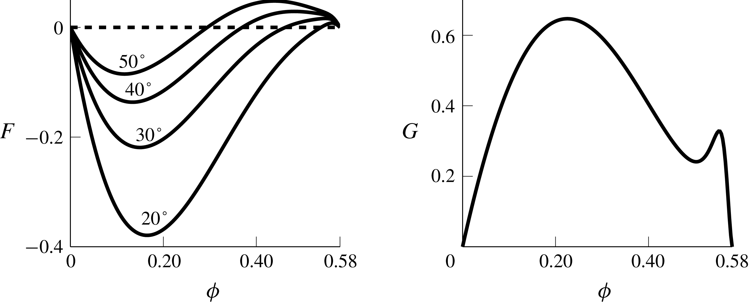
Flux
 $F(\unicode[STIX]{x1D719})$
(for selected angles) and
 $G(\unicode[STIX]{x1D719})$
in (2.34).

With further simplification, equation (2.25) reduces to a nonlinear convection–diffusion equation for
 $\unicode[STIX]{x1D719}$
on a fixed domain. Hereafter, we treat
 $\unicode[STIX]{x1D719}$
as a function of
 $\hat{z}$
and
 $\hat{t}$
only and consider
 ${\hat{h}}$
and depth-integrated concentration
 $\overline{\unicode[STIX]{x1D719}}$
to be constant. The scaled height, time and velocity are defined as
 $$\begin{eqnarray}s=\hat{z}/{\hat{h}},\quad \unicode[STIX]{x1D70F}=\hat{t}/{\hat{h}},\quad \tilde{u} ={\hat{h}}^{-2}\hat{u} ,\end{eqnarray}$$
the scaled shear stress as
 $$\begin{eqnarray}\unicode[STIX]{x1D70E}(s,\unicode[STIX]{x1D70F})=1-s+b\int _{s}^{1}\unicode[STIX]{x1D719}(\unicode[STIX]{x1D701},\unicode[STIX]{x1D70F})\,\text{d}\unicode[STIX]{x1D701}\end{eqnarray}$$
and the ratio of normal to suspension viscosity as
 $$\begin{eqnarray}R(\unicode[STIX]{x1D719})=\unicode[STIX]{x1D707}^{(n)}(\unicode[STIX]{x1D719})/\unicode[STIX]{x1D707}^{(s)}(\unicode[STIX]{x1D719}).\end{eqnarray}$$
We will assume here that
 $$\begin{eqnarray}R^{\prime }(\unicode[STIX]{x1D719})>0\text{ for }\unicode[STIX]{x1D719}>0,\lim _{\unicode[STIX]{x1D719}\rightarrow \unicode[STIX]{x1D719}_{m}}R(\unicode[STIX]{x1D719})<\infty ,\end{eqnarray}$$
which is satisfied, in particular, for the choices of
 $\hat{\unicode[STIX]{x1D707}}^{(n)},\hat{\unicode[STIX]{x1D707}}^{(s)}$
specified in (2.6) (note that for both viscosities, the order of the pole as
 $\unicode[STIX]{x1D719}\rightarrow \unicode[STIX]{x1D719}_{m}$
is
 $2$
, so their ratio remains finite (Boyer et al.
Reference Boyer, Pouliquen and Guazzelli2011)). It follows from the momentum equation (2.20) that
 $\tilde{u} _{s}\geqslant 0$
so
 $$\begin{eqnarray}(\hat{\unicode[STIX]{x1D707}}^{(n)}|\tilde{u} _{s}|)_{s}=(R(\unicode[STIX]{x1D719})\hat{\unicode[STIX]{x1D707}}^{(s)}\tilde{u} _{s})_{s}=(R(\unicode[STIX]{x1D719})\unicode[STIX]{x1D70E})_{s}.\end{eqnarray}$$
Equation (2.25) then becomes
 $$\begin{eqnarray}\unicode[STIX]{x1D719}_{\unicode[STIX]{x1D70F}}=(f_{h}(\unicode[STIX]{x1D719})[\unicode[STIX]{x1D6FD}\unicode[STIX]{x1D719}+(R(\unicode[STIX]{x1D719})\unicode[STIX]{x1D70E})_{s}])_{s},\end{eqnarray}$$
with
 $\unicode[STIX]{x1D70E}$
given by (2.28), which can also be written in the more standard form
 $$\begin{eqnarray}\unicode[STIX]{x1D719}_{\unicode[STIX]{x1D70F}}+F(\unicode[STIX]{x1D719})_{s}=(G(\unicode[STIX]{x1D719})\unicode[STIX]{x1D70E}\unicode[STIX]{x1D719}_{s})_{s},\end{eqnarray}$$
where (see figure 4)
 $$\begin{eqnarray}F(\unicode[STIX]{x1D719})=f_{h}(\unicode[STIX]{x1D719})\big(-\unicode[STIX]{x1D6FD}\unicode[STIX]{x1D719}+R(\unicode[STIX]{x1D719})(1+b\unicode[STIX]{x1D719})\big),\quad G(\unicode[STIX]{x1D719})=f_{h}(\unicode[STIX]{x1D719})R^{\prime }(\unicode[STIX]{x1D719}).\end{eqnarray}$$
We impose no-flux boundary conditions and assume that
 $\unicode[STIX]{x1D719}$
is initially uniform:
 $$\begin{eqnarray}\displaystyle & \displaystyle F=G\unicode[STIX]{x1D70E}\unicode[STIX]{x1D719}_{s}\quad \text{ at }s=0\text{ and }s=1, & \displaystyle\end{eqnarray}$$
 $$\begin{eqnarray}\displaystyle & \displaystyle \unicode[STIX]{x1D719}(s,0)=\overline{\unicode[STIX]{x1D719}}, & \displaystyle\end{eqnarray}$$
where
 $\overline{\unicode[STIX]{x1D719}}=\int _{0}^{1}\unicode[STIX]{x1D719}(s,\unicode[STIX]{x1D70F})\,\text{d}s$
is the total concentration. Due to (2.35), this value is constant.
Equations (2.33)–(2.36) form an initial-value problem for
 $\unicode[STIX]{x1D719}(s,\unicode[STIX]{x1D70F})$
, which we study numerically and approximately, foregoing a rigorous analysis of existence. Note that the diffusion coefficient
 $G\unicode[STIX]{x1D70E}$
degenerates when
 $\unicode[STIX]{x1D719}=0$
or
 $\unicode[STIX]{x1D719}_{m}$
and when
 $s=1$
(where the shear stress
 $\unicode[STIX]{x1D70E}$
is zero) and that (2.33) is not a standard diffusion equation since
 $G\unicode[STIX]{x1D70E}$
depends on an integral of
 $\unicode[STIX]{x1D719}$
.
As a technical note, the no-flux boundary condition (2.35) requires either
 $\unicode[STIX]{x1D719}=0,\unicode[STIX]{x1D719}=\unicode[STIX]{x1D719}_{c}$
or
 $\unicode[STIX]{x1D719}=\unicode[STIX]{x1D719}_{m}$
at the surface since
 $\unicode[STIX]{x1D70E}$
vanishes at
 $s=1.$
In reality, there should be an initial transient where
 $\unicode[STIX]{x1D719}(1,\unicode[STIX]{x1D70F})$
approaches one of these values, which is not within the scope of the model. As the transient does not affect the analysis that follows, we omit it for simplicity. The inconsistency can be resolved by the non-local shear rate at the surface (see appendix B).
2.3 Equilibrium profile: qualitative behaviour
As the equation is diffusive with no-flux boundary conditions, we expect that for each total concentration
 $\overline{\unicode[STIX]{x1D719}}$
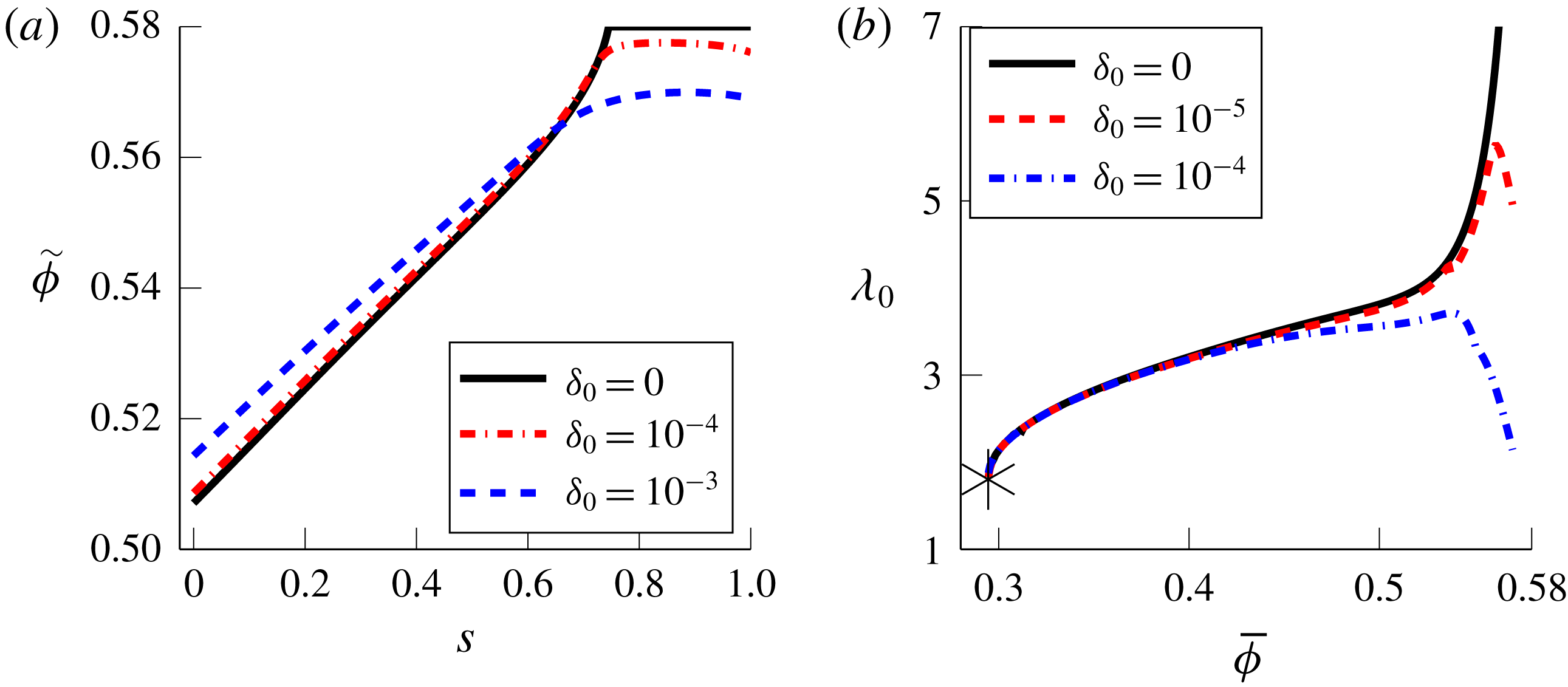
, there is a unique equilibrium profile
 $\widetilde{\unicode[STIX]{x1D711}}(s;\overline{\unicode[STIX]{x1D719}})$
to which all solutions to the initial value problem (2.33)–(2.36) converge as
 $\unicode[STIX]{x1D70F}\rightarrow \infty ,$
i.e. such that
 $$\begin{eqnarray}\lim _{\unicode[STIX]{x1D70F}\rightarrow \infty }\unicode[STIX]{x1D719}(s,\unicode[STIX]{x1D70F})=\widetilde{\unicode[STIX]{x1D711}}(s;\overline{\unicode[STIX]{x1D719}}).\end{eqnarray}$$
Numerically, we observe that this is true. The equilibrium profile
 $\widetilde{\unicode[STIX]{x1D711}}(s;\overline{\unicode[STIX]{x1D719}})$
is the solution to
 $$\begin{eqnarray}\unicode[STIX]{x1D719}_{s}=\frac{F(\unicode[STIX]{x1D719})}{G(\unicode[STIX]{x1D719})\unicode[STIX]{x1D70E}},\quad \int _{0}^{1}\unicode[STIX]{x1D719}\,\text{d}s=\overline{\unicode[STIX]{x1D719}},\end{eqnarray}$$
with
 $\unicode[STIX]{x1D70E}$
as given by (2.28). The properties of (2.38) are similar to those of the corresponding equilibrium equation derived using the diffusive flux model (e.g. Murisic et al.
Reference Murisic, Ho, Hu, Latterman, Koch, Lin, Mata and Bertozzi2011). In particular, if
 $\unicode[STIX]{x1D6FD}$
is not too large (i.e. the angle
 $\unicode[STIX]{x1D6FC}$
is not too small) then there is a critical concentration
 $\overline{\unicode[STIX]{x1D719}}_{c}\in (0,\unicode[STIX]{x1D719}_{m})$
satisfying
 $$\begin{eqnarray}0=F(\overline{\unicode[STIX]{x1D719}}_{c})=-\unicode[STIX]{x1D6FD}\overline{\unicode[STIX]{x1D719}}_{c}+(1+b\overline{\unicode[STIX]{x1D719}}_{c})R(\overline{\unicode[STIX]{x1D719}}_{c})\end{eqnarray}$$
for which the solution
 $\unicode[STIX]{x1D719}\equiv \overline{\unicode[STIX]{x1D719}}_{c}$
to (2.38) is constant. Moreover,
 $G\geqslant 0$
due to the assumption (2.30), so solutions are monotonically increasing with respect to
 $s$
if
 $\overline{\unicode[STIX]{x1D719}}>\overline{\unicode[STIX]{x1D719}}_{c}$
(‘ridged’) and monotonically decreasing with respect to
 $s$
if
 $\overline{\unicode[STIX]{x1D719}}<\overline{\unicode[STIX]{x1D719}}_{c}$
(‘settled’). If
 $\unicode[STIX]{x1D6FD}$
is large enough then
 $\overline{\unicode[STIX]{x1D719}}_{c}$
lies outside the physical range (
 $\overline{\unicode[STIX]{x1D719}}_{c}>\unicode[STIX]{x1D719}_{m}$
) so all solutions are settled.
To justify the use of the suspension balance model, we verify that the predicted critical concentration
 $\overline{\unicode[STIX]{x1D719}}_{c}$
is consistent with the diffusive flux approach and experimental results (Murisic et al.
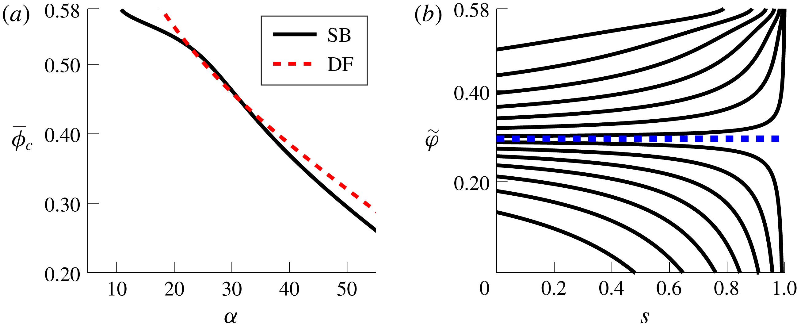
Reference Murisic, Ho, Hu, Latterman, Koch, Lin, Mata and Bertozzi2011). The critical concentration (as a function of
 $\unicode[STIX]{x1D6FC}$
) and typical equilibrium profiles are shown in figure 5, illustrating the close agreement. This also justifies the choice of
 $K_{n}\unicode[STIX]{x1D6EC}_{2}=0.8,$
which is the physical parameter that determines the critical concentration through
 $\unicode[STIX]{x1D6FD}$
in (2.39).
(a) Critical concentration
 $\overline{\unicode[STIX]{x1D719}}_{c}(\unicode[STIX]{x1D6FC})$
for
 $b=1.55$
for the suspension balance model derived here (‘SB’) and the diffusive flux model of Murisic et al. (Reference Murisic, Ho, Hu, Latterman, Koch, Lin, Mata and Bertozzi2011) for comparison (‘DF’). (b) Equilibrium profiles
 $\widetilde{\unicode[STIX]{x1D711}}(s;\overline{\unicode[STIX]{x1D719}})$
at various total concentrations
 $\overline{\unicode[STIX]{x1D719}}$
and
 $\unicode[STIX]{x1D6FC}=50^{\circ }$
(dashed line:
 $\overline{\unicode[STIX]{x1D719}}_{c}\approx 0.295$
).

It is worth noting, however, that at high concentrations, the two models are qualitatively different. Unlike the diffusive flux model, for which solutions are strictly less than
 $\unicode[STIX]{x1D719}_{m}$
except at
 $s=1$
, the equilibrium profile here may achieve a ‘packed’ layer with
 $\unicode[STIX]{x1D719}=\unicode[STIX]{x1D719}_{m}$
of finite thickness. The packed layer at exactly
 $\unicode[STIX]{x1D719}_{m}$
is a consequence of omitting the additional surface shear rate (Miller & Morris Reference Miller and Morris2006), which regularizes the solution and prevents formation of a packed layer (see appendix B).
3 Approach to
 $z$
-equilibrium

Here we estimate the time required for the particles to become close to equilibrium, starting from a uniform initial concentration. To be precise, we define the ‘
 $z$
-equilibration time’
 $\unicode[STIX]{x1D70F}_{eq}$
to be the time required for the
 $L^{2}$
error of the solution to the problem (2.33)–(2.36) to reach a fraction
 $\unicode[STIX]{x1D703}$
of its initial value, i.e. such that
 $$\begin{eqnarray}||\unicode[STIX]{x1D719}(\boldsymbol{\cdot },\unicode[STIX]{x1D70F})-\widetilde{\unicode[STIX]{x1D711}}||_{L^{2}}<\unicode[STIX]{x1D703}||\unicode[STIX]{x1D719}(\boldsymbol{\cdot },0)-\widetilde{\unicode[STIX]{x1D711}}||_{L^{2}}.\end{eqnarray}$$
We choose the
 $L^{2}$
norm for simplicity; in the settled regime, one could also use the difference between the fluid layer thickness and its equilibrium value, i.e.
 $$\begin{eqnarray}|s_{b}(\unicode[STIX]{x1D70F})-s_{b}^{\ast }|<\unicode[STIX]{x1D703}(1-s_{b}^{\ast }),\end{eqnarray}$$
with
 $s_{b}$
as defined in (3.3) (the top of the particle layer). The results that follow do not substantially change when using (3.2) in place of (3.1).
For the partial differential equation solution
 $\unicode[STIX]{x1D719}(s,\unicode[STIX]{x1D70F})$
we define the location of the ‘free boundary’ and its equilibrium value:
 $$\begin{eqnarray}s_{b}(\unicode[STIX]{x1D70F})=\sup \{s:0<\unicode[STIX]{x1D719}(s,\unicode[STIX]{x1D70F})<\unicode[STIX]{x1D719}_{m}\},\quad s_{b}^{\ast }:=\lim _{\unicode[STIX]{x1D70F}\rightarrow \infty }s_{b}(\unicode[STIX]{x1D70F}).\end{eqnarray}$$
The equilibrium solution degenerates in the interval
 $[s_{b}^{\ast },1]$
, with a value of either zero (settled) or
 $\unicode[STIX]{x1D719}_{m}$
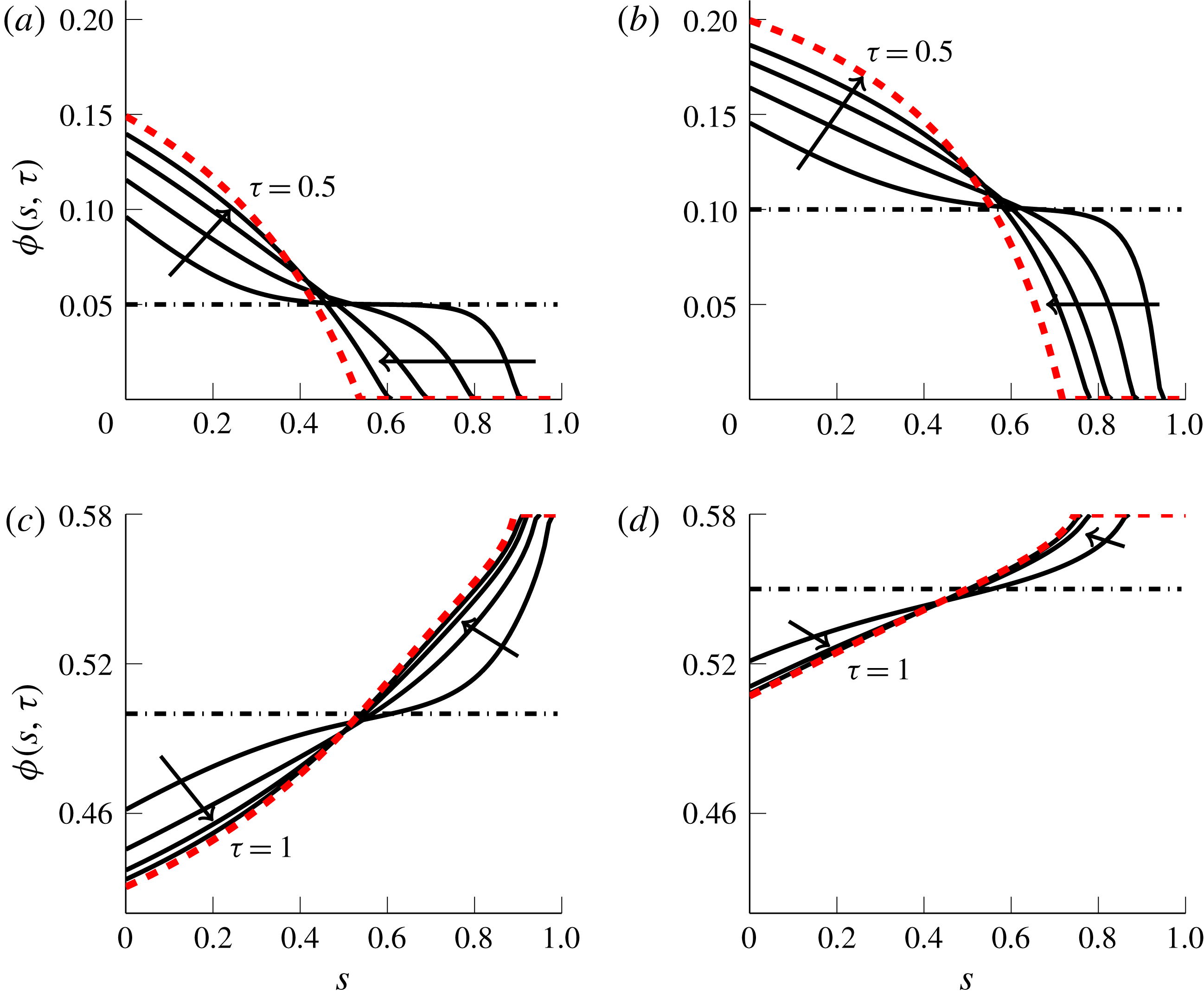
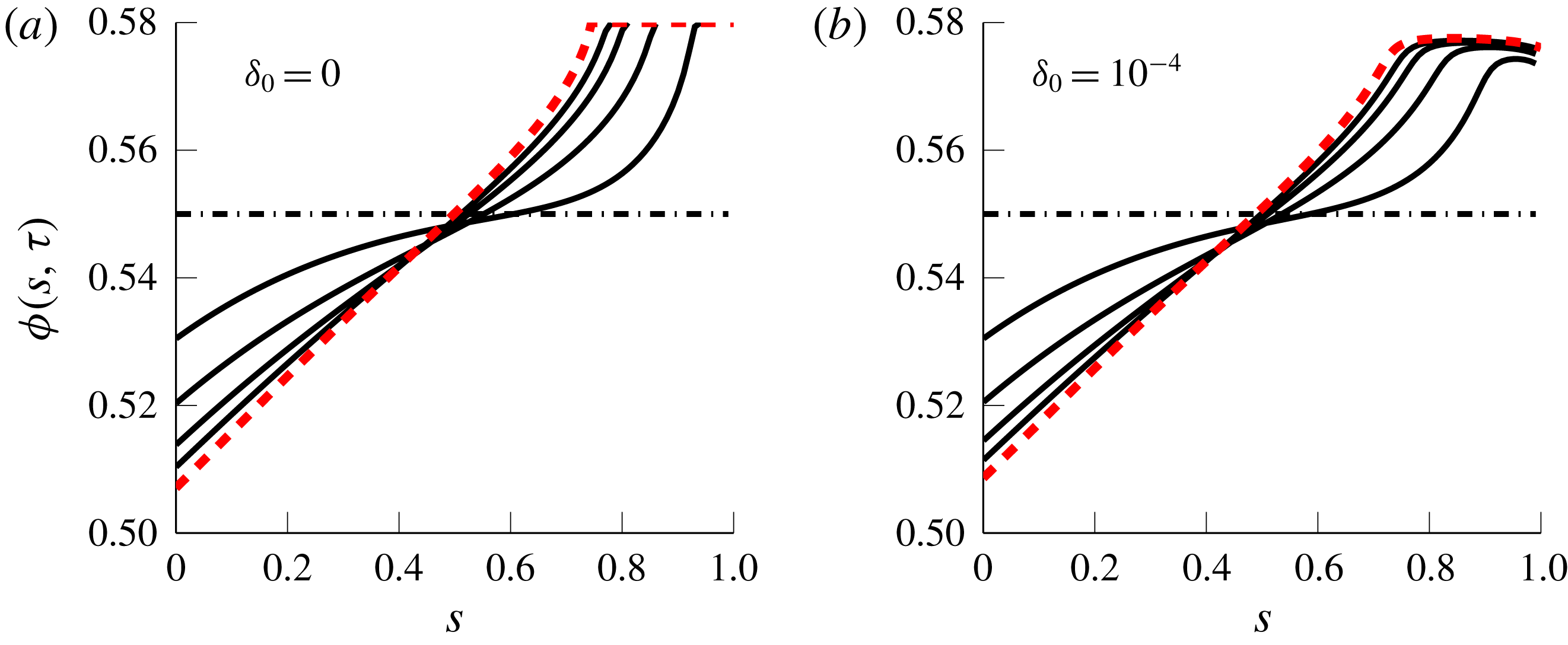
(ridged). The evolution of the particle profile has two qualitative phases, illustrated in figure 6:
(i) Descent phase: the free boundary
$s_{b}(\unicode[STIX]{x1D70F})$
recedes from
$s=1$
, decreasing towards
$s_{b}^{\ast }$
at an approximately linear rate.(ii) ‘Linear’ phase: once the solution is ‘close’ to the equilibrium
$\widetilde{\unicode[STIX]{x1D711}}$
, then the concentration will relax to
$\widetilde{\unicode[STIX]{x1D711}}$
, with the free boundary
$s_{b}(\unicode[STIX]{x1D70F})$
moving only a small amount.


The first phase corresponds to the formation of the top layer (clear fluid in the settled regime and a packed layer of particles in the ridged regime).
Note that the first phase is particular to the initially uniform concentration; for a different initial concentration such as a bed of particles that is resuspended into the fluid, the initial ascent/descent of particles towards the equilibrium will be different. However, the second phase is characterized by behaviour near the equilibrium, and is independent of the initial shape (depending only on
 $\overline{\unicode[STIX]{x1D719}}$
).
Evolution of concentration
 $\unicode[STIX]{x1D719}(s,\unicode[STIX]{x1D70F})$
from a flat initial state (dot-dashed) to the steady state (dashed) with
 $\unicode[STIX]{x1D6FC}=50^{\circ }$
from numerical simulation. (a,b) Settled;
 $\overline{\unicode[STIX]{x1D719}}=0.05$
and
 $\overline{\unicode[STIX]{x1D719}}=0.1$
up to
 $\unicode[STIX]{x1D70F}=0.5$
. (c,d) Ridged;
 $\overline{\unicode[STIX]{x1D719}}=0.5$
and
 $\overline{\unicode[STIX]{x1D719}}=0.55$
up to
 $\unicode[STIX]{x1D70F}=1$
. Arrows show increasing time.

We remark that the packed layer in the ridged regime is a consequence of the simple model; more realistically, it should be that
 $\unicode[STIX]{x1D719}$
is large but not quite
 $\unicode[STIX]{x1D719}_{m}$
due to the non-degeneracy of the shear rate at the surface (Miller & Morris Reference Miller and Morris2006). This means that defining the thickness of this high-concentration layer (where the particles accumulate near the surface) is somewhat more ambiguous and cannot be done through
 $s_{b}$
. As we do not perform the same detailed analysis as in the settled case, we do not pursue the analytical details here, although we briefly discuss the issue (in appendix B) and estimate the settling time only using the linear phase.
3.1 Linearization
Linearizing the partial differential equation about the equilibrium profile provides an estimate for the settling time in either regime. Near equilibrium, the
 $L^{2}$
distance between the equilibrium and
 $\unicode[STIX]{x1D719}(s,\unicode[STIX]{x1D70F})$
should decay like
 $\text{e}^{-\unicode[STIX]{x1D706}_{0}\unicode[STIX]{x1D70F}}$
for the minimum eigenvalue
 $\unicode[STIX]{x1D706}_{0}$
of the linearized problem. This provides an estimate for the equilibration time (3.1), given by
 $$\begin{eqnarray}\unicode[STIX]{x1D70F}_{eq}\approx \unicode[STIX]{x1D70F}_{eq}^{(l)}:=-\frac{\log \unicode[STIX]{x1D703}}{\unicode[STIX]{x1D706}_{0}}.\end{eqnarray}$$
To linearize, we fix a value
 $\overline{\unicode[STIX]{x1D719}}$
and consider the perturbation (with
 $\unicode[STIX]{x1D6FF}\ll 1$
a small parameter)
 $$\begin{eqnarray}\unicode[STIX]{x1D719}=\widetilde{\unicode[STIX]{x1D711}}(s)+\unicode[STIX]{x1D6FF}\text{e}^{-\unicode[STIX]{x1D706}\unicode[STIX]{x1D70F}}\unicode[STIX]{x1D713}^{\prime }(s),\quad \unicode[STIX]{x1D70E}=\int _{s}^{1}(1+b\unicode[STIX]{x1D719})\,\text{d}s^{\prime }=\tilde{\unicode[STIX]{x1D70E}}(s)-b\unicode[STIX]{x1D6FF}\text{e}^{-\unicode[STIX]{x1D706}\unicode[STIX]{x1D70F}}\unicode[STIX]{x1D713}(s),\end{eqnarray}$$
where
 $\widetilde{\unicode[STIX]{x1D711}}(s)$
is the equilibrium concentration. For simplicity, we ignore the effect of the moving boundary on convergence. This is justified a posteriori through numerical simulations that indicate that the effect of the boundary perturbation on the estimate can be neglected.
Substituting the ansatz into (2.32), we obtain the eigenvalue problem
 $$\begin{eqnarray}-f_{h}(\widetilde{\unicode[STIX]{x1D711}})(R^{\prime }(\widetilde{\unicode[STIX]{x1D711}})\tilde{\unicode[STIX]{x1D70E}}\unicode[STIX]{x1D713}^{\prime }+(\unicode[STIX]{x1D6FD}-bR(\widetilde{\unicode[STIX]{x1D711}}))\unicode[STIX]{x1D713})^{\prime }=\unicode[STIX]{x1D706}\unicode[STIX]{x1D713},\quad \unicode[STIX]{x1D713}(0)=\unicode[STIX]{x1D713}(1)=0,\end{eqnarray}$$
noting that the boundary conditions for
 $\unicode[STIX]{x1D713}$
follow from the fact that
 $\unicode[STIX]{x1D70E}(0)=1+b\overline{\unicode[STIX]{x1D719}}$
and
 $\unicode[STIX]{x1D70E}(1)=0$
. Under the assumptions (2.30) on
 $R$
, the diffusion coefficient
 $R^{\prime }\tilde{\unicode[STIX]{x1D70E}}$
for the linearized problem is non-negative, and so it follows by a simple calculation (see appendix A) that the eigenvalues are non-negative.
When the total concentration is at the critical value (
 $\overline{\unicode[STIX]{x1D719}}=\overline{\unicode[STIX]{x1D719}}_{c}$
), the equilibrium profile
 $\widetilde{\unicode[STIX]{x1D711}}\equiv \overline{\unicode[STIX]{x1D719}}_{c}$
is constant, permitting an exact solution. The eigenvalue problem (3.6) becomes
 $$\begin{eqnarray}-(A(1-s)\unicode[STIX]{x1D713}^{\prime }+B\unicode[STIX]{x1D713})^{\prime }=\unicode[STIX]{x1D706}\unicode[STIX]{x1D713},\quad \unicode[STIX]{x1D713}(0)=\unicode[STIX]{x1D713}(1)=0,\end{eqnarray}$$
where
 $A$
and
 $B$
are constants given by
 $$\begin{eqnarray}A=f_{h}(\overline{\unicode[STIX]{x1D719}}_{c})R^{\prime }(\overline{\unicode[STIX]{x1D719}}_{c})(1+b\overline{\unicode[STIX]{x1D719}}_{c}),\quad B=f_{h}(\overline{\unicode[STIX]{x1D719}}_{c})(\unicode[STIX]{x1D6FD}-bR(\overline{\unicode[STIX]{x1D719}}_{c}))=f_{h}(\overline{\unicode[STIX]{x1D719}}_{c})R(\overline{\unicode[STIX]{x1D719}}_{c})/\overline{\unicode[STIX]{x1D719}}_{c}.\end{eqnarray}$$
Defining
 $$\begin{eqnarray}\unicode[STIX]{x1D702}(\unicode[STIX]{x1D719})=\frac{\unicode[STIX]{x1D6FD}-bR(\unicode[STIX]{x1D719})}{R^{\prime }(\unicode[STIX]{x1D719})(1+b\unicode[STIX]{x1D719})},\quad \unicode[STIX]{x1D702}_{c}=\unicode[STIX]{x1D702}(\overline{\unicode[STIX]{x1D719}}_{c}),\end{eqnarray}$$
the general solution to (3.7) is
 $$\begin{eqnarray}\unicode[STIX]{x1D713}=k_{1}(1-s)^{\unicode[STIX]{x1D702}_{c}/2}\text{J}_{\unicode[STIX]{x1D702}_{c}}(2\sqrt{\unicode[STIX]{x1D706}(1-s)/A})+k_{2}(1-s)^{\unicode[STIX]{x1D702}_{c}/2}\text{Y}_{\unicode[STIX]{x1D702}_{c}}(2\sqrt{\unicode[STIX]{x1D706}(1-s)/A}),\end{eqnarray}$$
where
 $\text{J}_{\unicode[STIX]{x1D702}}$
and
 $\text{Y}_{\unicode[STIX]{x1D702}}$
are Bessel functions of the first and second kind, respectively. Note that
 $\unicode[STIX]{x1D6FD}-bR(\overline{\unicode[STIX]{x1D719}}_{c})=1/\overline{\unicode[STIX]{x1D719}}_{c}$
due to (2.39) and
 $R^{\prime }(\overline{\unicode[STIX]{x1D719}}_{c})>0$
by (2.30) so
 $\unicode[STIX]{x1D702}_{c}>0$
. It follows from this fact and the boundary conditions that
 $k_{2}=0$
, so the smallest eigenvalue is
 $$\begin{eqnarray}\unicode[STIX]{x1D706}_{0}(\overline{\unicode[STIX]{x1D719}}_{c})={\textstyle \frac{1}{4}}f_{h}(\overline{\unicode[STIX]{x1D719}}_{c})R^{\prime }(\overline{\unicode[STIX]{x1D719}}_{c})(1+b\overline{\unicode[STIX]{x1D719}}_{c})\unicode[STIX]{x1D6FE}(\unicode[STIX]{x1D702}_{c})^{2},\end{eqnarray}$$
where
 $\unicode[STIX]{x1D6FE}(\unicode[STIX]{x1D702})$
is the smallest positive zero of
 $\text{J}_{\unicode[STIX]{x1D702}}.$
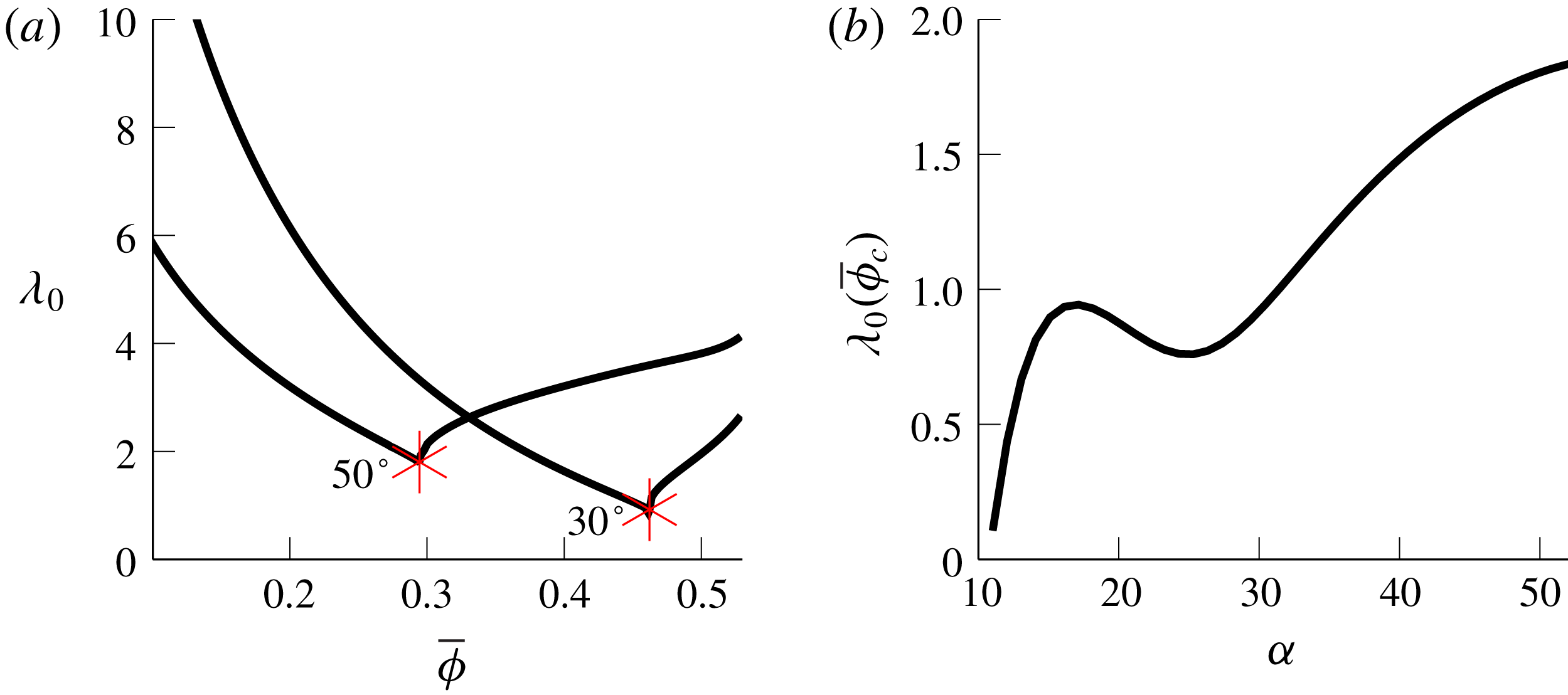
This ‘well-mixed’ eigenvalue (see figure 7) is the rate of convergence in the special case where the equilibrium profile is uniform (starting, of course, from a non-uniform initial profile). The peculiar local maximum of
 $\unicode[STIX]{x1D706}_{0}(\overline{\unicode[STIX]{x1D719}}_{c})$
for small angles
 $\unicode[STIX]{x1D6FC}$
(
 $\overline{\unicode[STIX]{x1D719}}_{c}$
near
 $\unicode[STIX]{x1D719}_{m}$
) in figure 7 is due to the sensitivity of the model functions
 $R^{\prime }$
and
 $f_{h}$
when
 $\unicode[STIX]{x1D719}$
is close to
 $\unicode[STIX]{x1D719}_{m}$
(which corresponds to
 $\unicode[STIX]{x1D6FC}\approx 15^{\circ }$
in the figure).
(a) Eigenvalue
 $\unicode[STIX]{x1D706}_{0}$
(solid) and well-mixed value at
 $\overline{\unicode[STIX]{x1D719}}_{c}$
(star) with
 $b=1.55$
at angles
 $\unicode[STIX]{x1D6FC}=30^{\circ }$
and
 $\unicode[STIX]{x1D6FC}=50^{\circ }$
. (b) Eigenvalue
 $\unicode[STIX]{x1D706}_{0}(\overline{\unicode[STIX]{x1D719}}_{c})$
in the well-mixed case given by (3.11) as a function of angle
 $\unicode[STIX]{x1D6FC}$
.

It is clear from the numerically computed eigenvalues (figure 7) that
 $\unicode[STIX]{x1D706}_{0}$
is decreasing with
 $\overline{\unicode[STIX]{x1D719}}$
for
 $\overline{\unicode[STIX]{x1D719}}<\overline{\unicode[STIX]{x1D719}}_{c}$
and increasing for
 $\overline{\unicode[STIX]{x1D719}}>\overline{\unicode[STIX]{x1D719}}_{c}$
. The value is minimized exactly at the critical concentration, which means that the well-mixed eigenvalue (3.11) is a lower bound on the convergence rate for a given inclination angle
 $\unicode[STIX]{x1D6FC}$
. However, an analytical proof of this result is missing, which would necessitate a more precise analysis of the eigenvalues as
 $\overline{\unicode[STIX]{x1D719}}\rightarrow \overline{\unicode[STIX]{x1D719}}_{c}$
.
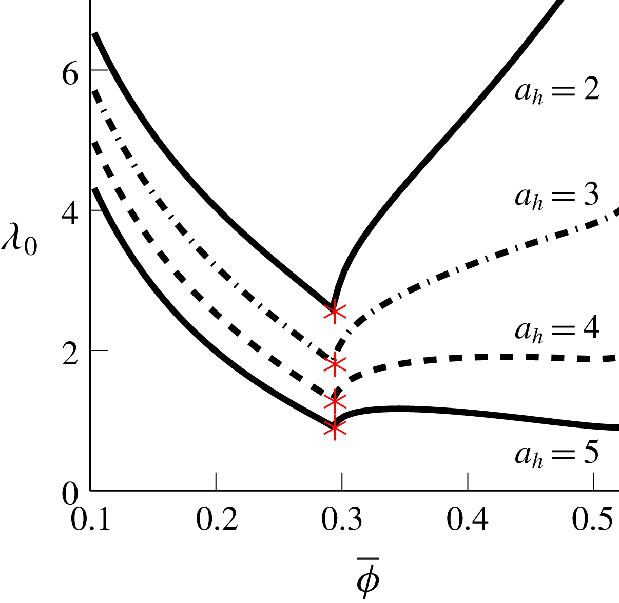
In figure 8 we show the effect of the hindrance function on the convergence rate by considering expressions of the form taking it to be
 $$\begin{eqnarray}f_{h}(\unicode[STIX]{x1D719})=(1-\unicode[STIX]{x1D719}/\unicode[STIX]{x1D719}_{m})(1-\unicode[STIX]{x1D719})^{a_{h}-1},\end{eqnarray}$$
with
 $a_{h}\in [2,5]$
. We observe that the predominant effect of the hindrance function
 $f_{h}$
in the settled regime is to scale the eigenvalues down as the exponent
 $a_{h}$
increases. The numerical computations suggest that the situation is more complicated in the ridged regime, where we speculate that the degeneracy in
 $f_{h}(\unicode[STIX]{x1D719})$
(as
 $\unicode[STIX]{x1D719}\rightarrow \unicode[STIX]{x1D719}_{m}$
) may become important.


3.2 Descent estimate
We now consider the descent phase in the settled regime, where the free boundary position
 $s_{b}(\unicode[STIX]{x1D70F})<1$
decreases towards
 $s_{b}^{\ast }.$
The particles settle, moving down towards their equilibrium state. The speed
 $s_{b}^{\prime }(\unicode[STIX]{x1D70F})$
of the free boundary is approximately constant during this phase, which yields an estimate for the settling time
 $\unicode[STIX]{x1D70F}_{eq}$
as
 $$\begin{eqnarray}\unicode[STIX]{x1D70F}_{eq}\approx (1-\unicode[STIX]{x1D703})\frac{1-s_{b}^{\ast }}{s_{b}^{\prime }}.\end{eqnarray}$$
To calculate this speed, observe that the system (2.33) and (2.28) with boundary condition
 $$\begin{eqnarray}\unicode[STIX]{x1D719}(1,\unicode[STIX]{x1D70F})=0\end{eqnarray}$$
(equivalent to the boundary condition (2.35) at
 $s=1$
) has a similarity solution
 $$\begin{eqnarray}\unicode[STIX]{x1D719}(s,t)=v\left(\frac{1-s}{\unicode[STIX]{x1D70F}}\right)=v(\unicode[STIX]{x1D709}),\end{eqnarray}$$
where
 $v$
satisfies the ordinary differential equation
 $$\begin{eqnarray}-\unicode[STIX]{x1D709}\frac{\text{d}v}{\text{d}\unicode[STIX]{x1D709}}-\frac{\text{d}}{\text{d}\unicode[STIX]{x1D709}}F(v)=\frac{\text{d}}{\text{d}\unicode[STIX]{x1D709}}\left(G(v)\left(\int _{0}^{\unicode[STIX]{x1D709}}(1+bv(\unicode[STIX]{x1D701}))\,\text{d}\unicode[STIX]{x1D701}\right)\frac{\text{d}v}{\text{d}\unicode[STIX]{x1D709}}\right)\end{eqnarray}$$
and boundary condition
 $v(0)=0.$
Setting
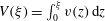 $V(\unicode[STIX]{x1D709})=\int _{0}^{\unicode[STIX]{x1D709}}v(z)\,\text{d}z$
and integrating from
 $0$
to
 $\unicode[STIX]{x1D709}$
and using that
 $F(0)=0$
we obtain
 $$\begin{eqnarray}-\unicode[STIX]{x1D709}V^{\prime }+V-F(V^{\prime })=G(V^{\prime })(\unicode[STIX]{x1D709}+bV)V^{\prime \prime },\quad V(0)=V^{\prime }(0)=0.\end{eqnarray}$$
We define, for each solution to (3.17), the quantity
 $$\begin{eqnarray}\unicode[STIX]{x1D709}_{0}=\inf \{\unicode[STIX]{x1D709}:v(\unicode[STIX]{x1D709})>0\}.\end{eqnarray}$$
Observe that if the similarity solution is valid near the free boundary (where
 $\unicode[STIX]{x1D719}=0$
), then according to the definition (3.15), this boundary will descend at a speed
 $\unicode[STIX]{x1D709}_{0}.$
However, the bounded domain poses difficulties, since the similarity ordinary differential equation is incompatible with the boundary condition at
 $s=0$
. To obtain a useful solution, we instead consider
 $\unicode[STIX]{x1D719}$
in the half-infinite domain
 $(-\infty ,1]$
and impose the far-field boundary condition
 $$\begin{eqnarray}\lim _{s\rightarrow -\infty }\unicode[STIX]{x1D719}=\overline{\unicode[STIX]{x1D719}}.\end{eqnarray}$$
In terms of the similarity variable, this condition becomes
 $$\begin{eqnarray}\lim _{\unicode[STIX]{x1D709}\rightarrow \infty }v(\unicode[STIX]{x1D709})=\overline{\unicode[STIX]{x1D719}}.\end{eqnarray}$$
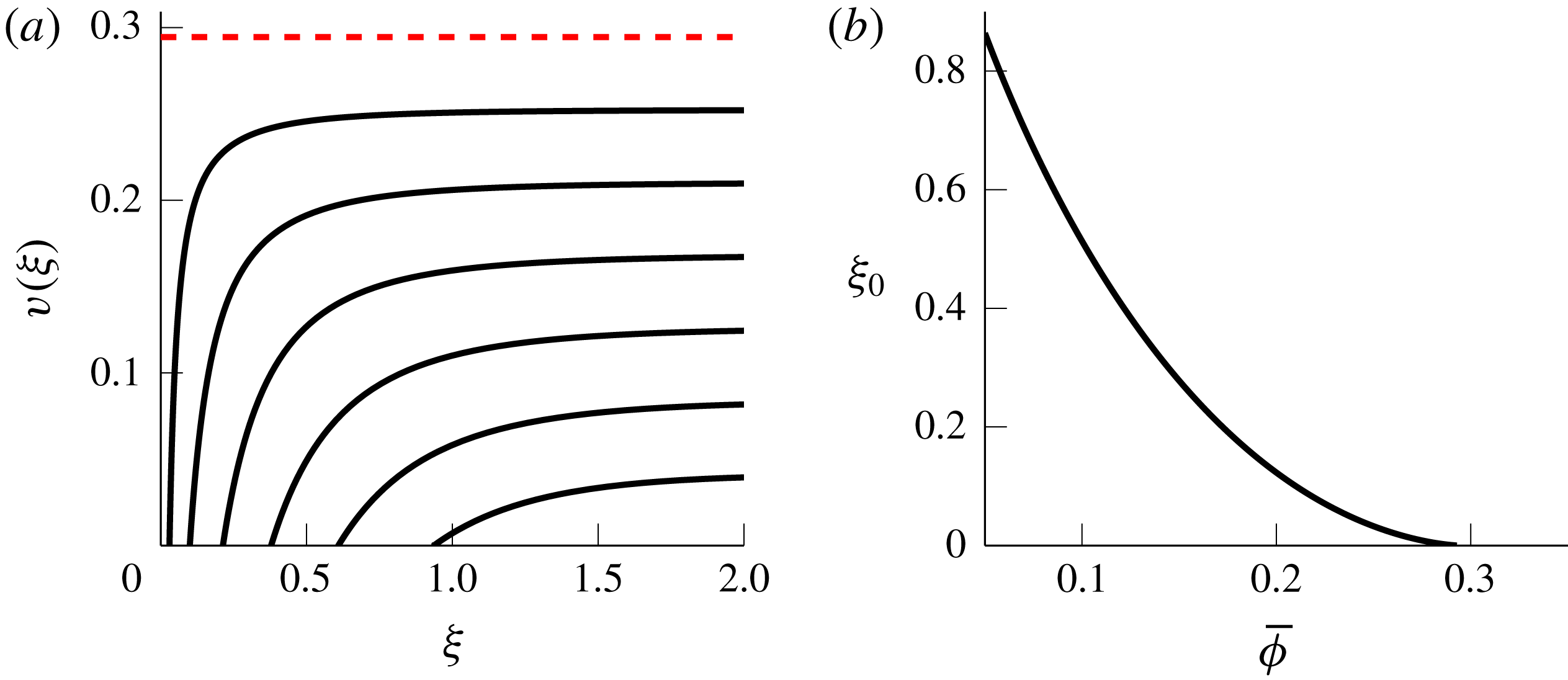
Solutions to the ordinary differential equation (3.17) with the far-field boundary condition (3.20) appear to be a one-parameter family of solutions
 $V(\unicode[STIX]{x1D709};\overline{\unicode[STIX]{x1D719}})$
whose support is the interval
 $[\unicode[STIX]{x1D709}_{0}(\overline{\unicode[STIX]{x1D719}}),\infty )$
as shown in figure 9.
(a) With
 $\unicode[STIX]{x1D709}=(1-s)/t$
, similarity solutions
 $\unicode[STIX]{x1D719}(s,\unicode[STIX]{x1D70F})=v(\unicode[STIX]{x1D709})=V^{\prime }(\unicode[STIX]{x1D709})$
with
 $V$
solving (3.17) for various limiting values
 $\overline{\unicode[STIX]{x1D719}}=\lim _{\unicode[STIX]{x1D709}\rightarrow \infty }v$
at
 $\unicode[STIX]{x1D6FC}=50^{\circ }$
(dashed line:
 $\overline{\unicode[STIX]{x1D719}}_{c}\approx 0.29$
). (b) Corresponding values of the descent speed
 $\unicode[STIX]{x1D709}_{0}$
, which approaches zero as
 $\overline{\unicode[STIX]{x1D719}}\rightarrow \overline{\unicode[STIX]{x1D719}}_{c}$
.

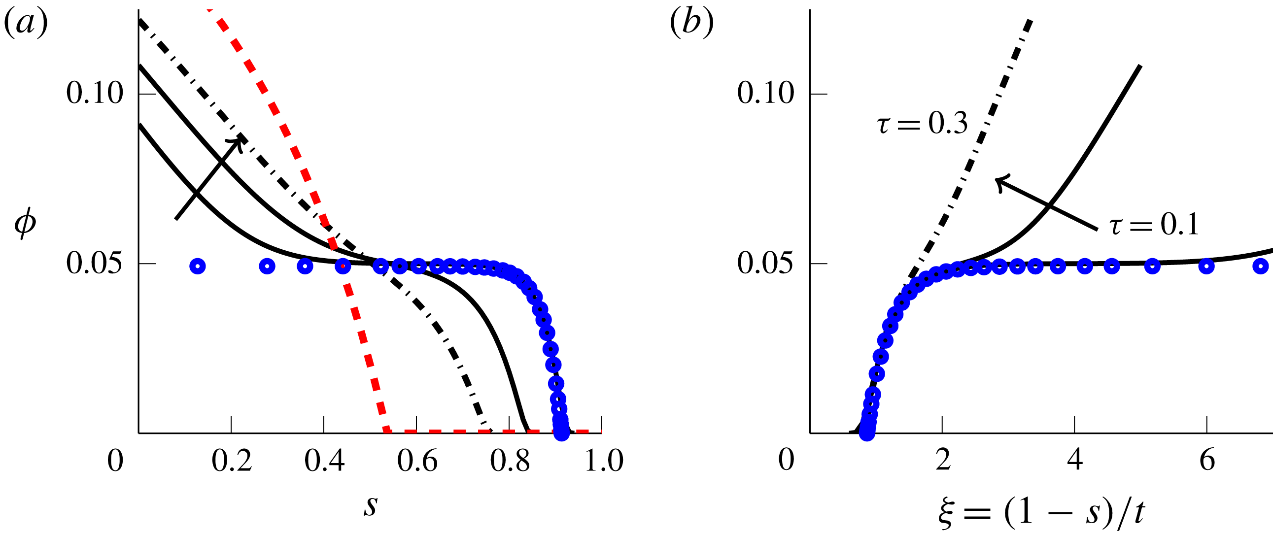
The validity of the similarity solution near the free boundary is illustrated in figure 10. As time varies, the solutions
 $\unicode[STIX]{x1D719}(s,\unicode[STIX]{x1D70F})$
collapse onto the similarity solution
 $v(\unicode[STIX]{x1D709})$
close to the free boundary (
 $\unicode[STIX]{x1D709}=\unicode[STIX]{x1D709}_{0}$
or
 $s=s_{b}(\unicode[STIX]{x1D70F})$
). So long as the solution near the free boundary connects to a locally constant region at the value
 $\overline{\unicode[STIX]{x1D719}}$
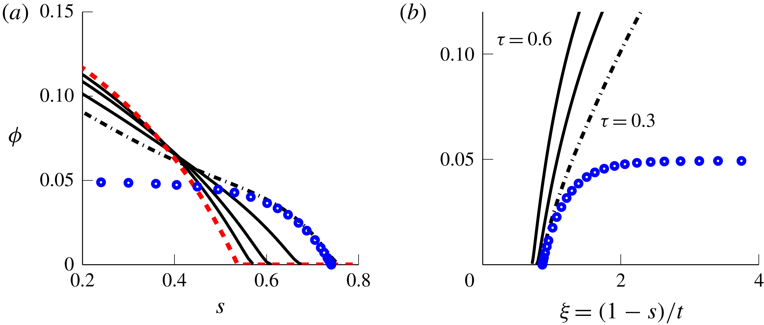
, the similarity solution remains a valid approximation for the descent speed. Eventually, the flat region disappears (figure 11), so the far-field condition (3.20) is no longer appropriate and the similarity solution ceases to be valid; this signifies the end of the descent phase.
Concentration profile (solid and dot-dashed lines) and similarity solution
 $v(\unicode[STIX]{x1D709})$
(circles) at early times as defined in (3.15) (parameters:
 $\overline{\unicode[STIX]{x1D719}}=0.05$
and
 $\unicode[STIX]{x1D6FC}=50^{\circ }$
). The dashed line is the equilibrium profile; dot-dashed line is
 $\unicode[STIX]{x1D719}(s,\unicode[STIX]{x1D70F})$
at
 $\unicode[STIX]{x1D70F}=0.3$
. At early times, the similarity solution is accurate near the free boundary.

Concentration profile (solid and dot-dashed lines) and similarity solution
 $v(\unicode[STIX]{x1D709})$
(circles) at later times (parameters:
 $\overline{\unicode[STIX]{x1D719}}=0.05$
and
 $\unicode[STIX]{x1D6FC}=50^{\circ }$
). The dashed line is the equilibrium profile; dot-dashed line is
 $\unicode[STIX]{x1D719}(s,\unicode[STIX]{x1D70F})$
at
 $\unicode[STIX]{x1D70F}=0.3$
. The locally constant region with
 $\unicode[STIX]{x1D719}=\overline{\unicode[STIX]{x1D719}}$
vanishes at
 $\unicode[STIX]{x1D70F}\approx 0.3$
, which means that the far-field approximation
 $\lim _{s\rightarrow -\infty }\unicode[STIX]{x1D719}=\overline{\unicode[STIX]{x1D719}}$
no longer applies.

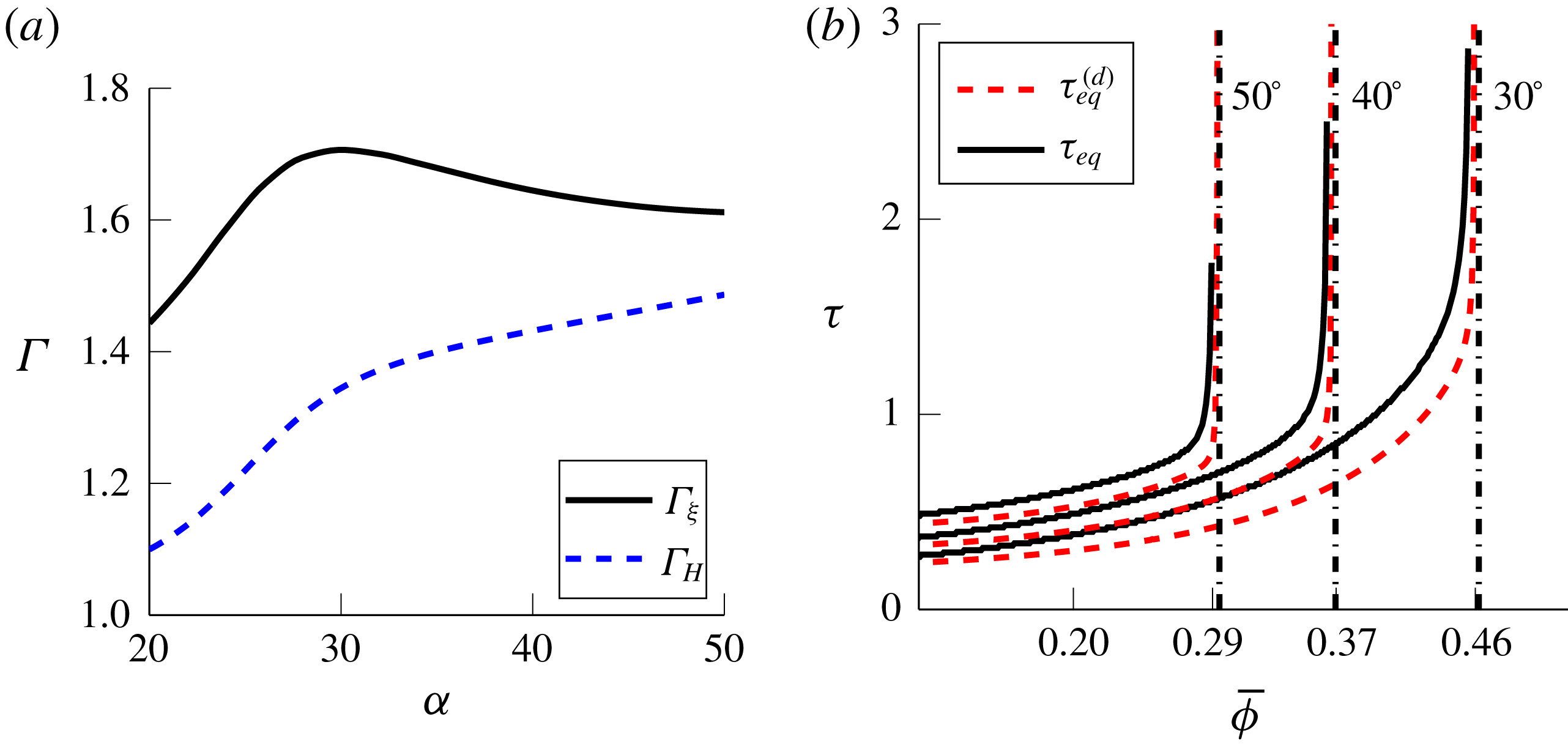
(a) Exponents
 $\unicode[STIX]{x1D6E4}_{\unicode[STIX]{x1D709}}$
and
 $\unicode[STIX]{x1D6E4}_{H}$
for (3.23) as a function of angle for
 $b=1.55$
; the equilibration time should diverge as
 $\overline{\unicode[STIX]{x1D719}}{\nearrow}\overline{\unicode[STIX]{x1D719}}_{c}$
if
 $\unicode[STIX]{x1D6E4}_{\unicode[STIX]{x1D709}}>\unicode[STIX]{x1D6E4}_{H}$
. (b) Descent estimate
 $\unicode[STIX]{x1D70F}_{eq}^{(d)}$
and settling time
 $\unicode[STIX]{x1D70F}_{eq}$
at various angles and
 $\unicode[STIX]{x1D703}=0.2$
; the dashed vertical line is at
 $\overline{\unicode[STIX]{x1D719}}_{c}$
for the corresponding curve.

3.3 Discussion of convergence estimates
Substituting
 $\unicode[STIX]{x1D709}_{0}$
into (3.13) yields the convergence estimate
 $$\begin{eqnarray}\unicode[STIX]{x1D70F}_{eq}\approx \unicode[STIX]{x1D70F}_{eq}^{(d)}:=(1-\unicode[STIX]{x1D703})\frac{1-s_{b}^{\ast }}{\unicode[STIX]{x1D709}_{0}}.\end{eqnarray}$$
This estimate behaves quite differently from the linear estimate (3.4) when
 $\overline{\unicode[STIX]{x1D719}}$
is close to
 $\overline{\unicode[STIX]{x1D719}}_{c}$
, capturing the dramatic increase in settling time in this limit. Recall from § 2.3 (see figure 5) that in the settled regime the equilibrium fluid layer thickness
 $$\begin{eqnarray}H_{f}=1-s_{b}^{\ast }\end{eqnarray}$$
decreases to zero as
 $\overline{\unicode[STIX]{x1D719}}$
increases to
 $\overline{\unicode[STIX]{x1D719}}_{c}$
. It is evident from numerical calculations that
 $$\begin{eqnarray}\unicode[STIX]{x1D709}_{0}\sim C_{1}(\overline{\unicode[STIX]{x1D719}}_{c}-\overline{\unicode[STIX]{x1D719}})^{\unicode[STIX]{x1D6E4}_{\unicode[STIX]{x1D709}}},\quad \unicode[STIX]{x1D6E4}_{H}\sim C_{2}(\overline{\unicode[STIX]{x1D719}}_{c}-\overline{\unicode[STIX]{x1D719}})^{\unicode[STIX]{x1D6E4}_{H}}\quad \text{as }\overline{\unicode[STIX]{x1D719}}{\nearrow}\overline{\unicode[STIX]{x1D719}}_{c}\end{eqnarray}$$
for exponents
 $\unicode[STIX]{x1D6E4}_{\unicode[STIX]{x1D709}},\unicode[STIX]{x1D6E4}_{H}$
that depend on
 $\unicode[STIX]{x1D6FC}.$
This suggests that
 $$\begin{eqnarray}\unicode[STIX]{x1D70F}_{eq}\sim C(\overline{\unicode[STIX]{x1D719}}_{c}-\overline{\unicode[STIX]{x1D719}})^{\unicode[STIX]{x1D6E4}_{H}-\unicode[STIX]{x1D6E4}_{\unicode[STIX]{x1D709}}}\quad \text{as }\overline{\unicode[STIX]{x1D719}}{\nearrow}\overline{\unicode[STIX]{x1D719}}_{c}\end{eqnarray}$$
and so the settling time should diverge as
 $\overline{\unicode[STIX]{x1D719}}$
approaches the critical concentration if
 $\unicode[STIX]{x1D6E4}_{\unicode[STIX]{x1D709}}>\unicode[STIX]{x1D6E4}_{H}$
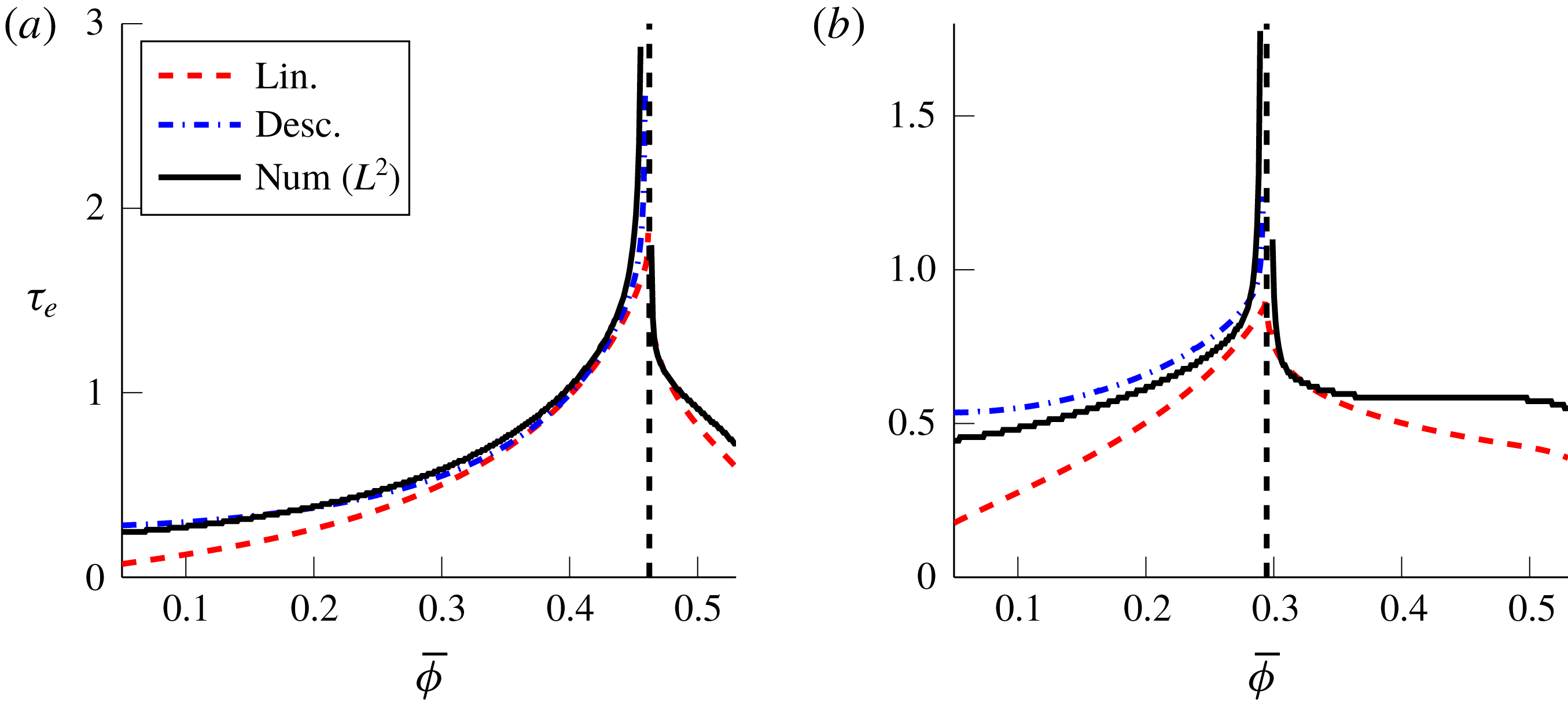
, i.e. if the fluid layer thickness shrinks in size slower than the descent velocity. As shown in figure 12, the settling time
 $\unicode[STIX]{x1D70F}_{eq}$
calculated from numerical simulations (solid line) is consistent with this divergence.
A plot of the exponents
 $\unicode[STIX]{x1D6E4}_{\unicode[STIX]{x1D709}}$
and
 $\unicode[STIX]{x1D6E4}_{H}$
as a function of angle for
 $b=1.55$
is shown in figure 12 along with the estimate
 $\unicode[STIX]{x1D70F}_{eq}^{(d)}$
for the settling time
 $\unicode[STIX]{x1D70F}_{eq}$
at some sample angles. Note that
 $\unicode[STIX]{x1D6E4}_{\unicode[STIX]{x1D709}}>\unicode[STIX]{x1D6E4}_{H}$
for all values of
 $\unicode[STIX]{x1D6FC}$
, but that the difference is small (at most
 $0.35$
for the range of angles where
 $\overline{\unicode[STIX]{x1D719}}_{c}$
exists in figure 12, for instance), so the dramatic growth in equilibration time occurs only very close to
 $\overline{\unicode[STIX]{x1D719}}_{c}$
. For other values of
 $b>0$
, the situation is similar. We do not have a theoretical estimate for the exponents
 $\unicode[STIX]{x1D6E4}_{\unicode[STIX]{x1D709}}$
and
 $\unicode[STIX]{x1D6E4}_{H}$
, which would provide a condition determining when time diverges to infinity or converges to zero. Nevertheless, there is a clear increase over a wide range of physically realistic parameters, consistent with observations of past experiments (Murisic et al.
Reference Murisic, Ho, Hu, Latterman, Koch, Lin, Mata and Bertozzi2011).
The descent estimate (3.21) (plotted in figure 13) is most relevant when the equilibrium layer thickness
 $H_{f}$
is large relative to the descent speed, which holds both in the dilute limit (when
 $H_{f}\approx 1$
) and near
 $\overline{\unicode[STIX]{x1D719}}_{c}$
(where
 $H_{f}$
is small but the speed is much smaller). Notably, the preceding analysis suggests that
 $$\begin{eqnarray}\lim _{\overline{\unicode[STIX]{x1D719}}{\nearrow}\overline{\unicode[STIX]{x1D719}}_{c}}\unicode[STIX]{x1D70F}_{eq}^{(l)}=\text{const.},\quad \lim _{\overline{\unicode[STIX]{x1D719}}{\nearrow}\overline{\unicode[STIX]{x1D719}}_{c}}\unicode[STIX]{x1D70F}_{eq}^{(d)}=\infty .\end{eqnarray}$$
The calculations in figure 12 indicate that the divergence predicted for
 $\unicode[STIX]{x1D70F}_{eq}^{(d)}$
is indeed the correct behaviour for
 $\unicode[STIX]{x1D70F}_{eq}$
. However, this growth is only noticeable in a narrow window, since the exponent
 $\unicode[STIX]{x1D6E4}_{H}-\unicode[STIX]{x1D6E4}_{\unicode[STIX]{x1D709}}$
in (3.24) is negative but small.
Comparison of convergence estimates
 $\unicode[STIX]{x1D70F}_{eq}^{(l)}$
and
 $\unicode[STIX]{x1D70F}_{eq}^{(d)}$
((3.4) and (3.21), respectively) with a threshold
 $\unicode[STIX]{x1D703}=0.2$
and numerically computed settling time
 $\unicode[STIX]{x1D70F}_{eq}$
using the
 $L^{2}$
norm. (a) Angle
 $\unicode[STIX]{x1D6FC}=30^{\circ }$
; a small angle with
 $\overline{\unicode[STIX]{x1D719}}_{c}$
near
 $\unicode[STIX]{x1D719}_{m}$
. (b) Angle
 $\unicode[STIX]{x1D6FC}=50^{\circ }$
; a large angle with
 $\overline{\unicode[STIX]{x1D719}}_{c}$
at a moderate value. The dashed vertical line is at
 $\overline{\unicode[STIX]{x1D719}}_{c}$
.

4 Connection to bulk flow
Here we aim to obtain a simple heuristic for the transition distance
 ${\mathcal{L}}$
(as depicted in figure 3) using the equilibration model. For the bulk flow, the model equations (2.14) and conservation of fluid/particle mass yield conservation laws for the film height
 $h(x,t)$
and
 $\overline{\unicode[STIX]{x1D719}}(x,t)$
(Murisic et al.
Reference Murisic, Pausader, Peschka and Bertozzi2013) which are, in dimensional form,
 $$\begin{eqnarray}\displaystyle & \displaystyle 0=h_{t}+\left(\int _{0}^{h}u\,\text{d}z\right)_{x}, & \displaystyle\end{eqnarray}$$
 $$\begin{eqnarray}\displaystyle & \displaystyle 0=(h\overline{\unicode[STIX]{x1D719}})_{t}+\left(\int _{0}^{h}\unicode[STIX]{x1D719}u\,\text{d}z\right)_{x}. & \displaystyle\end{eqnarray}$$
 $z$
-equilibration takes place. This decouples the two processes, and we can then estimate the transition distance as the point at which the particles are within some threshold of their
 $z$
-equilibrium.
4.1 Transition time and distance
Consider a fixed area
 $A$
of an initially uniform mixture released from a reservoir and allowed to flow down an incline (see figure 3). Assume that the suspension height
 $h(x,t)$
and leading edge
 $x_{f}(t)$
evolve in a well-mixed state while the equilibration process occurs. The flow is then that of an effective fluid with viscosity
 $\unicode[STIX]{x1D707}(\overline{\unicode[STIX]{x1D719}})$
as given by (2.6) and density
 $\unicode[STIX]{x1D70C}(\overline{\unicode[STIX]{x1D719}})=1+b\overline{\unicode[STIX]{x1D719}}$
. The conservation laws (4.1) reduce, in dimensional form, to
 $$\begin{eqnarray}h_{t}+\frac{g\sin \unicode[STIX]{x1D6FC}}{3\unicode[STIX]{x1D708}_{\ell }\hat{\unicode[STIX]{x1D708}}(\overline{\unicode[STIX]{x1D719}})}(h^{3})_{x}=0,\end{eqnarray}$$
where
 $$\begin{eqnarray}\hat{\unicode[STIX]{x1D708}}(\unicode[STIX]{x1D719}):=\frac{\hat{\unicode[STIX]{x1D707}}^{(s)}(\unicode[STIX]{x1D719})}{1+b\unicode[STIX]{x1D719}}\end{eqnarray}$$
is the effective kinematic viscosity relative to
 $\unicode[STIX]{x1D708}_{\ell }$
. The height profile of the uniform suspension, after the formation of the rarefaction–shock pair, is given by (Huppert Reference Huppert1982)
 $$\begin{eqnarray}h=\left\{\begin{array}{@{}ll@{}}(x/(c_{f}t))^{1/2},\quad & x<x_{f}(t),\\ 0,\quad & x>x_{f}(t),\end{array}\right.\quad x_{f}(t)=(9c_{f}A^{2}t/4)^{1/3},\end{eqnarray}$$
where
 $A$
is the initial area of the fluid and
 $$\begin{eqnarray}c_{f}=g\sin \unicode[STIX]{x1D6FC}/(\unicode[STIX]{x1D708}_{\ell }\hat{\unicode[STIX]{x1D708}}(\overline{\unicode[STIX]{x1D719}})).\end{eqnarray}$$
Now suppose that the
 $z$
-equilibration process is occurring at the front
 $x_{f}(t)$
while the height changes (which affects the process only through the time scale
 $T_{e}$
for equilibration (2.19)). We then estimate that the transition time
 $t_{e}$
is the time required for this process at the front to reach a threshold
 $\unicode[STIX]{x1D703}$
of equilibrium as defined in § 3.
Given a length scale
 $L$
, we define an estimate
 ${\mathcal{L}}$
for the non-dimensional transition distance as follows:
 $$\begin{eqnarray}{\mathcal{L}}=x_{f}(t_{e})/L.\end{eqnarray}$$
The effect of the changing height on the equilibration time scale
 $T_{e}$
and time variable
 $\unicode[STIX]{x1D70F}$
is taken into account by using
 $h(x_{f}(t))$
as the instantaneous height scale. The relevant time scale is proportional to the height at the front. We denote
 $H$
the initial height scale and
 $T_{e}$
the time scale based on this initial height. Then at each time
 $t$
, the height at the front induces a dimensionless time scale over which the system can evolve. Relating these time scales, we have
 $$\begin{eqnarray}\text{d}\unicode[STIX]{x1D70F}=\frac{H}{h(x_{f}(t))T_{e}}\,\text{d}t=\frac{H}{T_{e}}\left(\frac{2c_{f}}{3A}\right)^{1/3}t^{1/3}.\end{eqnarray}$$
Thus a step forward of
 $\text{d}t$
in dimensional units brings about a time step
 $\propto 1/h$
in dimensionless time units
 $\text{d}\unicode[STIX]{x1D70F}$
. Thus the dimensional settling time
 $t_{e}$
and settling time
 $\unicode[STIX]{x1D70F}_{eq}$
defined in (3.1) are related by
 $$\begin{eqnarray}\unicode[STIX]{x1D70F}_{eq}=\int _{0}^{\unicode[STIX]{x1D70F}_{eq}}\,\text{d}\unicode[STIX]{x1D70F}=\frac{H}{T_{e}}\int _{0}^{t_{e}}\frac{1}{h(x_{f}(t))}\,\text{d}t=\frac{3H}{4T_{e}}\left(\frac{2c_{f}}{3A}\right)^{1/3}t_{e}^{4/3}.\end{eqnarray}$$
The transition distance (4.6) is then, using (2.19), (4.4) and (4.5) to simplify,
 $$\begin{eqnarray}\displaystyle {\mathcal{L}}=\frac{1}{L}\left(\frac{9A^{2}}{4}\left(\left(\frac{24}{K_{n}\unicode[STIX]{x1D6EC}_{2}d^{2}}\frac{\unicode[STIX]{x1D70F}_{eq}}{\hat{\unicode[STIX]{x1D708}}}\right)^{3}\frac{3A}{2}\right)^{1/4}\right)^{1/3}, & & \displaystyle\end{eqnarray}$$
noting that the explicit factor of
 $\sin \unicode[STIX]{x1D6FC}$
cancels, but
 ${\mathcal{L}}$
does depend on angle through the value of
 $\unicode[STIX]{x1D70F}_{eq}=\unicode[STIX]{x1D70F}_{eq}(\overline{\unicode[STIX]{x1D719}},\unicode[STIX]{x1D6FD})$
determined by the equilibration process described in § 3 (in particular,
 $\unicode[STIX]{x1D70F}_{eq}$
is a function of
 $\overline{\unicode[STIX]{x1D719}}$
and the parameter
 $\unicode[STIX]{x1D6FD}$
(2.26)). Upon simplifying, we arrive at an expression for the transition distance as a function of mixture concentration
 $\overline{\unicode[STIX]{x1D719}}$
and incline angle
 $\unicode[STIX]{x1D6FC}$
:
 $$\begin{eqnarray}{\mathcal{L}}(\overline{\unicode[STIX]{x1D719}},\unicode[STIX]{x1D6FC})=\left(\left(\frac{81A^{3}}{K_{n}\unicode[STIX]{x1D6EC}_{2}L^{4}d^{2}}\right)\frac{\unicode[STIX]{x1D70F}_{eq}(\unicode[STIX]{x1D719},\unicode[STIX]{x1D6FD}(\unicode[STIX]{x1D6FC}))}{\hat{\unicode[STIX]{x1D708}}(\unicode[STIX]{x1D719})}\right)^{1/4}.\end{eqnarray}$$
Note that
 ${\mathcal{L}}$
depends on angle only through the parameter
 $\unicode[STIX]{x1D6FD}$
in the equilibration time. To get a more concrete formula for
 ${\mathcal{L}}$
, we then replace
 $\unicode[STIX]{x1D70F}_{eq}$
with one of the estimates
 $\unicode[STIX]{x1D70F}_{eq}^{(l)}$
or
 $\unicode[STIX]{x1D70F}_{eq}^{(d)}$
from the linearized or descent processes ((3.4) and (3.21), respectively).
It is useful to interpret the result using the asymptotic assumption on the particles:
 $$\begin{eqnarray}\unicode[STIX]{x1D716}H^{2}/d^{2}\ll 1.\end{eqnarray}$$
We define the parameter
 $$\begin{eqnarray}\unicode[STIX]{x1D6FF}:=\left(\frac{81}{K_{n}\unicode[STIX]{x1D6EC}_{2}}\frac{\unicode[STIX]{x1D716}H^{2}}{d^{2}}\right)^{1/4}.\end{eqnarray}$$
We choose
 $H$
and
 $L$
to be the height/length of the reservoir (so
 $A=HL$
). Then (4.10) becomes
 $$\begin{eqnarray}{\mathcal{L}}=\unicode[STIX]{x1D6FF}\left(\frac{\unicode[STIX]{x1D70F}_{eq}}{\hat{\unicode[STIX]{x1D708}}}\right)^{1/4}.\end{eqnarray}$$
Thus if
 $\unicode[STIX]{x1D6FF}\ll 1$
(the limit of very fast equilibration) then
 ${\mathcal{L}}\ll 1$
. However, if the size difference is not so small (moderately fast equilibration) then
 ${\mathcal{L}}$
may be larger than
 $1$
, i.e. the suspension may stay well-mixed for a distance of the order of the length scale
 $L$
. To be precise, the estimate suggests that the length
 ${\mathcal{L}}$
will be significant despite the ‘fast’ equilibration when
 $$\begin{eqnarray}\frac{K_{n}\unicode[STIX]{x1D6EC}_{2}}{81}\lesssim \frac{\unicode[STIX]{x1D716}H^{2}}{d^{2}}\ll 1,\end{eqnarray}$$
noting that
 $\unicode[STIX]{x1D6EC}_{2}=0.8$
.
For a suspension with a constant input flux forming a film of height
 $H$
, the estimate is simpler. The solution to (4.2) is then a shock that travels at a constant speed
 $U/3$
, from which it follows that
 $$\begin{eqnarray}{\mathcal{L}}=\frac{T_{e}U}{3L}\frac{\unicode[STIX]{x1D70F}_{eq}}{\hat{\unicode[STIX]{x1D708}}}=\unicode[STIX]{x1D6FF}\frac{\unicode[STIX]{x1D70F}_{eq}}{\hat{\unicode[STIX]{x1D708}}},\quad \unicode[STIX]{x1D6FF}:=\frac{6}{K_{n}\unicode[STIX]{x1D6EC}_{2}}\left(\frac{\unicode[STIX]{x1D716}H^{2}}{d^{2}}\right),\end{eqnarray}$$
which can be interpreted in the same way (
 ${\mathcal{L}}\sim 1$
when
 $\unicode[STIX]{x1D716}H^{2}/d^{2}\sim K_{n}\unicode[STIX]{x1D6EC}_{2}/6$
). Alternatively,
 $$\begin{eqnarray}{\mathcal{L}}=\frac{T_{e}}{3T_{B}}\frac{\unicode[STIX]{x1D70F}_{eq}}{\hat{\unicode[STIX]{x1D708}}},\end{eqnarray}$$
where
 $T_{B}=L/U$
is the bulk time scale.
4.2 Comparison to experiments
We now wish to use this notion of
 ${\mathcal{L}}$
to understand experiments where a suspension in this asymptotic regime is observed to remain well-mixed over the distance of the experimental track for some concentrations and angles. The ‘well-mixed band’ for the experiments in Murisic et al. (Reference Murisic, Ho, Hu, Latterman, Koch, Lin, Mata and Bertozzi2011) consists of the region in the
 $(\overline{\unicode[STIX]{x1D719}},\unicode[STIX]{x1D6FC})$
plane where the suspension remained well-mixed until it reached a distance of approximately 0.6 m down the track.
Based on our model assumptions, the predictions we make for
 ${\mathcal{L}}$
are independent of the suspending fluid (kinematic) viscosity
 $\unicode[STIX]{x1D708}_{\ell }$
. However, the inclusion of higher-order effects may include such dependence (there is a small viscosity dependence observed in experiments). Here we compare to the results of experiment B in Murisic et al. (Reference Murisic, Ho, Hu, Latterman, Koch, Lin, Mata and Bertozzi2011), in which the fluid viscosity is fixed at
 $\unicode[STIX]{x1D708}_{\ell }=1000~\text{cSt}$
and three particle sizes are considered: small (
 $d=0.143~\text{mm}$
), moderate (
 $d=0.337~\text{mm}$
) and large (
 $d=0.625~\text{mm}$
).
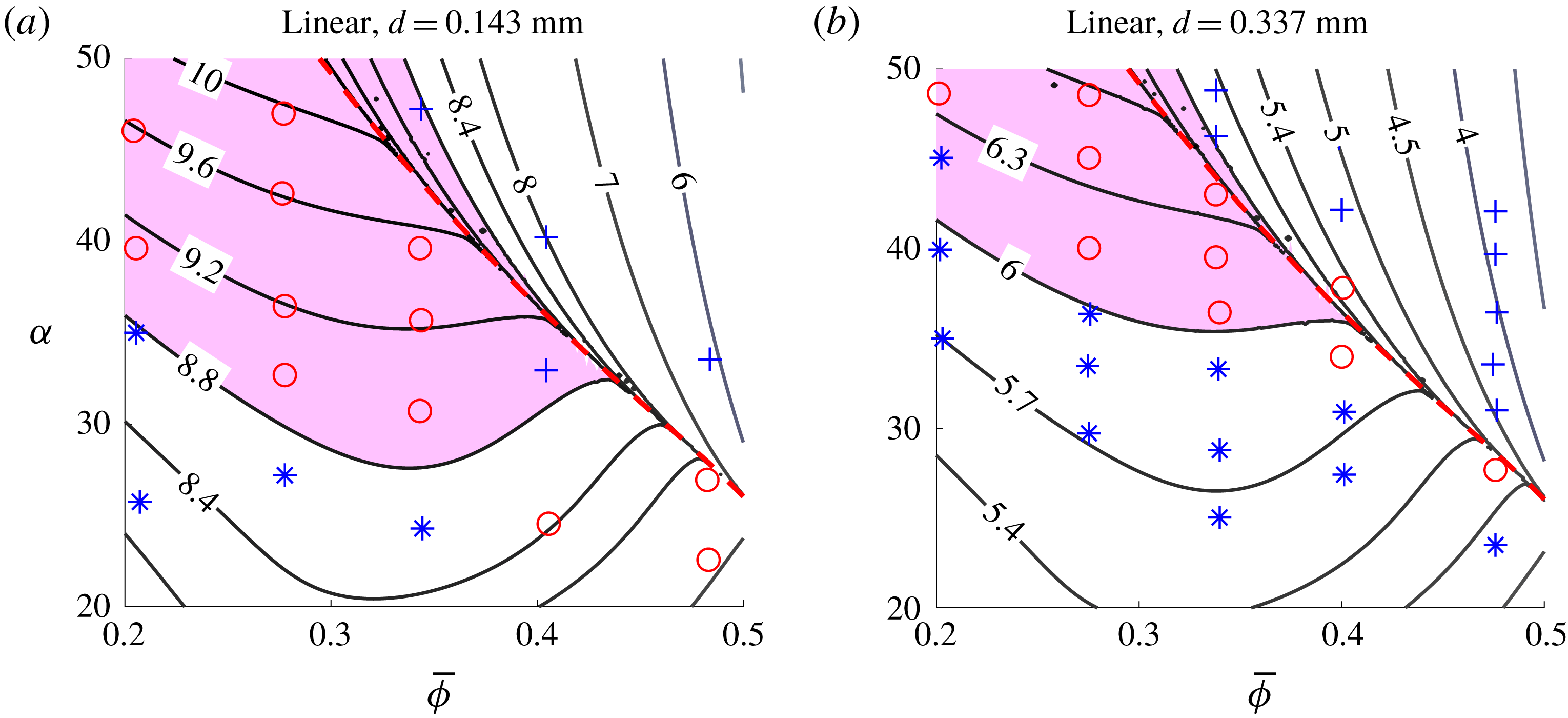
Contours of the transition distance
 ${\mathcal{L}}(\overline{\unicode[STIX]{x1D719}},\unicode[STIX]{x1D6FC})$
of (4.13) using the linearized estimate (3.4) compared to experimental data in Murisic et al. (Reference Murisic, Ho, Hu, Latterman, Koch, Lin, Mata and Bertozzi2011) for small particles with a wide well-mixed band (a) and larger particles (b). Stars, circles and pluses represent, respectively, ‘settled’, ‘mixed’ and ‘ridged’ suspensions when observed at
 $0.6~\text{m}$
(which corresponds to
 ${\mathcal{L}}=6$
). The shaded region is the the best fit to the well-mixed band (the expected set is
 $\{{\mathcal{L}}\geqslant 6\}$
). The convergence threshold
 $\unicode[STIX]{x1D703}=0.08$
was chosen to match the
 $d=0.337~\text{mm}$
band.

To compare, we take the length scale to be
 $L=0.1~\text{m}$
(the reservoir length) and
 $b=1.55,$
an initial area of
 $A\approx 1\times 10^{-3}~\text{m}^{2}$
and
 $\unicode[STIX]{x1D719}_{m}=0.58.$
The ‘well-mixed band’ in the experiment corresponds to the set
 $\{{\mathcal{L}}>6\}.$
The convergence threshold
 $\unicode[STIX]{x1D703}=0.08$
is chosen to match the moderate particle size. For the small and moderate particle size, the experimental well-mixed band is plotted against the value of
 ${\mathcal{L}}$
in figure 14. The shape of the well-mixed band for the linear estimate, which is wider (in
 $\overline{\unicode[STIX]{x1D719}}$
) for larger angles, is consistent with the experimental data, except near the critical concentration and at small angle, where it tapers sharply. The cutoff value for the small particles that matches the data is larger than
 ${\mathcal{L}}=6$
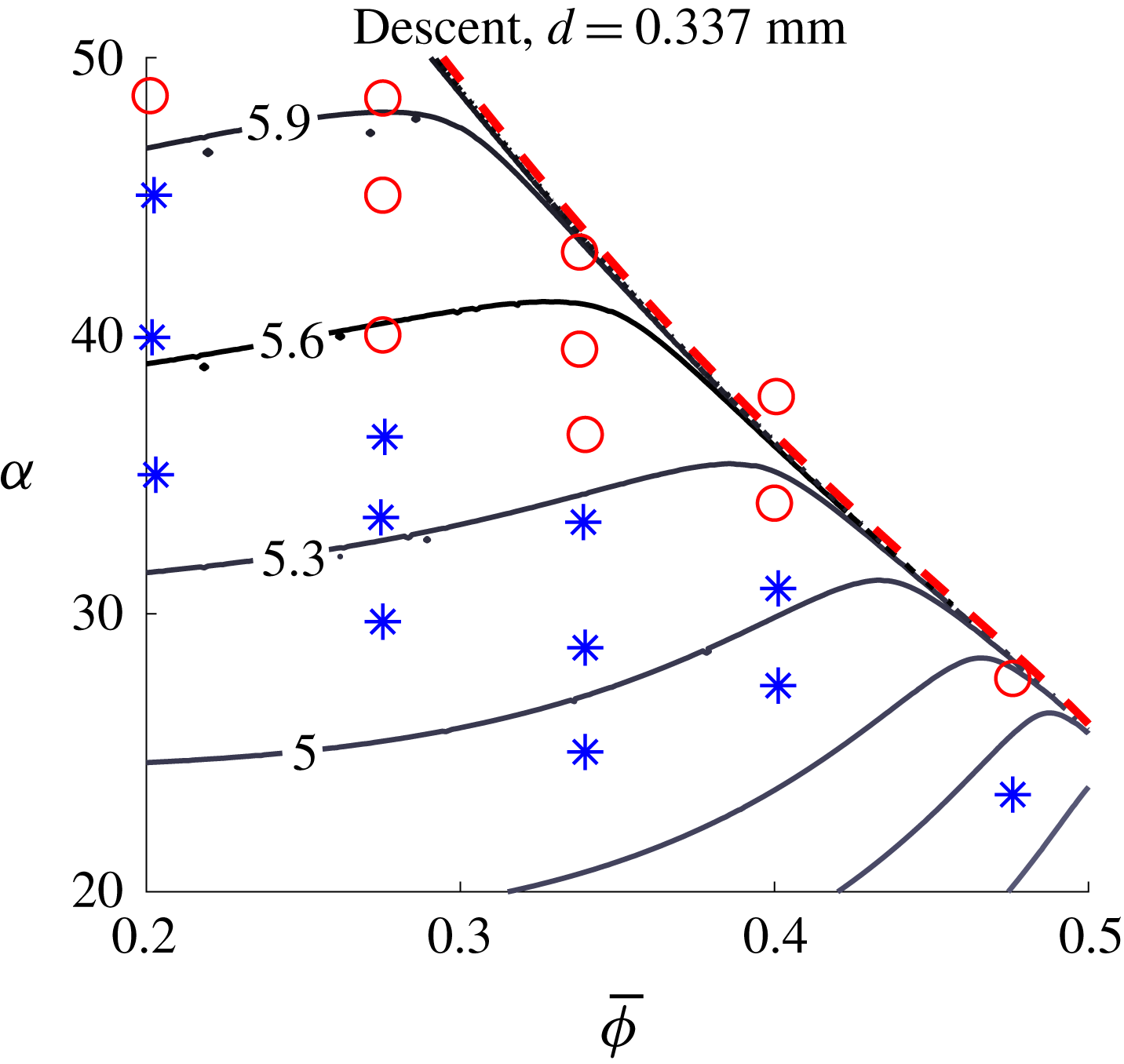
, which does not match as well (though the shape is reasonable). The descent estimate (figure 15) predicts a well-mixed band of a different shape that does not match experimental observations. Note that the contour lines are asymptotically parallel to the critical concentration line
 $\overline{\unicode[STIX]{x1D719}}_{c}(\unicode[STIX]{x1D6FC})$
, which is a consequence of the fact that
 $\unicode[STIX]{x1D70F}_{eq}^{(d)}\rightarrow \infty$
as
 $\overline{\unicode[STIX]{x1D719}}{\nearrow}\overline{\unicode[STIX]{x1D719}}_{c}.$
The overall size of the well-mixed band is similar to that predicted by the linear estimate, but the lower bound is nearly flat. From the better fit of the linearized estimate, it seems that the relaxation to equilibrium rather than the descent phase is the primary mechanism for the transition distance.
Contours for the transition distance
 ${\mathcal{L}}$
using the descent estimate (3.21) with threshold
 $\unicode[STIX]{x1D703}=0.08$
compared to experimental data in Murisic et al. (Reference Murisic, Ho, Hu, Latterman, Koch, Lin, Mata and Bertozzi2011) (see figure 14 for key); the expected well-mixed band is
 $\{{\mathcal{L}}\geqslant 6\}$
. We observe a poorer fit to the data compared to the linearized estimate, both in value and in qualitative shape.

Note that, since
 $(\unicode[STIX]{x1D70F}_{eq}^{(l)}/\hat{\unicode[STIX]{x1D708}})^{1/4}$
is bounded above, we predict that the well-mixed band should vanish if the particle size
 $d$
is large enough. That is, for large enough particles and a fixed track length, the particles will always equilibrate by the time the suspension reaches the end of the track. For experiments considered here, this corresponds to the condition that (4.13) is less than
 $6$
for all relevant
 $\overline{\unicode[STIX]{x1D719}}$
and
 $\unicode[STIX]{x1D6FC}$
. We obtain
 $$\begin{eqnarray}d_{\mathit{max}}\approx \frac{1}{{\mathcal{L}}^{2}}\max _{\unicode[STIX]{x1D6FC},\overline{\unicode[STIX]{x1D719}}}\left(\frac{81A^{3}}{K_{n}\unicode[STIX]{x1D6EC}_{2}L^{4}}\frac{\unicode[STIX]{x1D70F}_{eq}^{(l)}}{\hat{\unicode[STIX]{x1D708}}}\right)^{1/2}\approx 0.407~\text{mm},\end{eqnarray}$$
with
 ${\mathcal{L}}=6$
and the maximum taken over
 $\unicode[STIX]{x1D6FC}\in [20^{\circ },50^{\circ }]$
and
 $\overline{\unicode[STIX]{x1D719}}\in [0.2,0.5]$
. The data in Murisic et al. (Reference Murisic, Ho, Hu, Latterman, Koch, Lin, Mata and Bertozzi2011) also show the well-mixed band vanishing, finding it absent with
 $d=0.625~\text{mm}$
.
5 Conclusion
When a uniform mixture of a viscous suspension is poured onto an incline, there is a transient distance over which the particles migrate in the shear flow to either settle or rise to the surface, depending on the balance of forces. Beyond this transient distance, the resulting stratification of particles in the normal direction determines the evolution of the bulk flow. Our work here has focused on the transient dynamics that precede the developed flow, using a suspension balance model to study the particle equilibration on a fast time scale. From a uniform initial state in the settled regime, this process takes place in two qualitatively distinct phases: the formation of a clear fluid layer as the particles descend from the free surface at roughly constant speed and the relaxation of the near-equilibrium particle distribution to its final state, which is described by the slowest decaying mode of the linearized system.
The speed of the particle descent was understood by means of a local similarity solution, which shows that at the beginning of the settling process, the clear fluid layer does descend at a roughly constant rate (consistent with numerical computations). Using this analysis, we found the equilibration time for particle descent diverges near the critical concentration; however, such analysis yielded well-mixed bands that did not agree with experimental observations. Using the linearized system, we found better agreement with data. We therefore hypothesize that the particle descent may only be a short-lived phenomenon that blends into a diffusive equilibration process, the latter ultimately governing the settling time and length. Given the correct apparatuses, it should be possible to observe and study these processes in experiments.
The rough estimate for the equilibration length provides some insight into its dependence on physical parameters. In particular, we note that even when the
 $z$
-equilibration time scale is fast, the length travelled while mixed may be substantial. However, the estimate requires some crude assumptions on the evolution of the flow to simplify the estimate. Mathematically, it would be fruitful to study the fully coupled system for the transient flow – without assuming quasi-static evolution in either direction – and/or to carefully study some approximate (asymptotic) solutions that take into account both the fast and long time scales inherent to the system. Our analysis of the equilibrium profile for the particles and its stability was limited to the fast time scale; it would be interesting to study the influence of the downstream flow on the stability of the particle layer or the effect of the particles on the stability of the advancing fronts through analysis of the coupled system.
From a modelling perspective, this paper has shed light on the fast-time-scale dynamics in the settled regime, but the dynamics for dense suspensions (the ridged regime) remains to be explored in depth. The complications in the model introduced by the surface particle concentration approaching maximum packing warrant further study; a different model may be necessary to consider the formation of such particle layers at the surface and their effect on the equilibration dynamics.
Acknowledgements
M.L. received support from the Natural Sciences and Engineering Research Council of Canada (NSERC) (funding reference no. PDF-502-479-2017). Cette recherche a été financée par le Conseil de recherches en sciences naturelles et en génie du Canada (CRSNG) (numéro de référence PDF-502-479-2017). A.L.B. was supported by a Simons Foundation Math +X Inv. Award no. 510776. The authors acknowledge the experimental work of P. Flynn, J. Pappe, A. Prins, W. Sisson, S. Stanton and R. Yang as a motivation for this study. The authors would also like to thank the reviewers for valuable suggestions.
Appendix A. Spectrum for the linearized problem
Here we provide the details for the linearized eigenvalue problem (3.6) in the settled regime as discussed in § 3.1. We wish to verify that the eigenvalue problem is of a standard form and has positive eigenvalues. Suppose
 $\overline{\unicode[STIX]{x1D719}}<\overline{\unicode[STIX]{x1D719}}_{c}$
, so there is a degeneracy where the solution reaches
 $\unicode[STIX]{x1D719}=0$
but no point at which
 $\unicode[STIX]{x1D719}=\unicode[STIX]{x1D719}_{m}.$
Define coefficients
 $A(s)$
and
 $B(s)$
as
 $$\begin{eqnarray}A(s)=R^{\prime }(\widetilde{\unicode[STIX]{x1D711}}(s))\widetilde{\unicode[STIX]{x1D70E}}(s),\quad B(s)=\unicode[STIX]{x1D6FD}-bR(\widetilde{\unicode[STIX]{x1D711}}(s))\end{eqnarray}$$
so that (3.6) has the form
 $$\begin{eqnarray}-(A(s)\unicode[STIX]{x1D713}^{\prime }+B(s)\unicode[STIX]{x1D713})^{\prime }=\frac{\unicode[STIX]{x1D706}}{f_{h}(\widetilde{\unicode[STIX]{x1D711}}(s))}\unicode[STIX]{x1D713},\quad \unicode[STIX]{x1D713}(0)=\unicode[STIX]{x1D713}(1)=0.\end{eqnarray}$$
Recall that the support of
 $\widetilde{\unicode[STIX]{x1D711}}$
is
 $[0,s_{b}^{\ast }]$
in the settled regime, with
 $s_{b}^{\ast }<1.$
Thus
 $A(s)$
vanishes for
 $s>s_{b}^{\ast }$
. We look for a solution with
 $\unicode[STIX]{x1D713}=0$
for
 $s>s_{b}^{\ast }$
, i.e. to instead solve
 $$\begin{eqnarray}-(A(s)\unicode[STIX]{x1D713}^{\prime }+B(s)\unicode[STIX]{x1D713})^{\prime }=\frac{\unicode[STIX]{x1D706}}{f_{h}}\unicode[STIX]{x1D713},\quad \unicode[STIX]{x1D713}(0)=\unicode[STIX]{x1D713}(s_{b}^{\ast })=0\end{eqnarray}$$
for which
 $A(s)>0$
except at the right endpoint
 $s=s_{b}^{\ast }.$
In the interior, define
 $$\begin{eqnarray}E(s)=\exp \left(-\int _{0}^{s}\frac{B(x)}{A(x)}\,\text{d}x\right).\end{eqnarray}$$
From the equilibrium theory (§ 2.3), we have that
 $$\begin{eqnarray}\lim _{s{\nearrow}s^{\ast }}\widetilde{\unicode[STIX]{x1D711}}^{\prime }(s)=-\frac{\unicode[STIX]{x1D6FD}}{R^{\prime \prime }(0)(1-s_{b}^{\ast })}\end{eqnarray}$$
from which it follows that as
 $s{\nearrow}s_{b}^{\ast }$
,
 $$\begin{eqnarray}\displaystyle A(s) & = & \displaystyle R^{\prime }(\widetilde{\unicode[STIX]{x1D711}}(s))\widetilde{\unicode[STIX]{x1D70E}}(s)\nonumber\\ \displaystyle & = & \displaystyle R^{\prime \prime }(0)\widetilde{\unicode[STIX]{x1D70E}}(s_{b}^{\ast })\widetilde{\unicode[STIX]{x1D711}}^{\prime }(s_{b}^{\ast })(s-s_{b}^{\ast })+O((s-s_{b}^{\ast })^{2})\nonumber\\ \displaystyle & = & \displaystyle -\unicode[STIX]{x1D6FD}(s-s_{b}^{\ast })+O((s-s_{b}^{\ast })^{2}).\end{eqnarray}$$
Since
 $B\sim \unicode[STIX]{x1D6FD}$
(a non-zero constant) as
 $s{\nearrow}s_{b}^{\ast }$
we have
 $$\begin{eqnarray}E(s)\sim \exp \left(O(s)+\int _{0}^{s}1/(x-s_{b}^{\ast })\,\text{d}x\right)\sim C(s_{b}^{\ast }-s)\quad \text{as }s{\nearrow}s_{b}^{\ast }.\end{eqnarray}$$
We can place the eigenvalue problem in a standard self-adjoint form by defining
 $$\begin{eqnarray}p=AE,\quad r=E/f_{h},\quad \unicode[STIX]{x1D712}=\unicode[STIX]{x1D713}/E.\end{eqnarray}$$
This gives a (singular) self-adjoint problem for
 $\unicode[STIX]{x1D712}$
:
 $$\begin{eqnarray}-(p\unicode[STIX]{x1D712}^{\prime })^{\prime }=r\unicode[STIX]{x1D706}\unicode[STIX]{x1D712},\quad \unicode[STIX]{x1D712}(0)=0.\end{eqnarray}$$
From (A 7), the coefficients have the following behaviour as
 $s{\nearrow}s_{b}^{\ast }$
:
 $$\begin{eqnarray}p\sim C\unicode[STIX]{x1D6FD}(s-s_{b}^{\ast })^{2},\quad r\sim C(s-s_{b}^{\ast }).\end{eqnarray}$$
Since the operator is formally self-adjoint with mild singularities on the coefficients, we expect a spectrum of positive eigenvalues with a minimum eigenvalue
 $\unicode[STIX]{x1D706}_{0}$
(Zettl Reference Zettl2005). Since
 $p\geqslant 0$
and
 $\unicode[STIX]{x1D712}(0)=p(s_{b}^{\ast })=0,$
this eigenvalue is positive.
Appendix B. Non-local shear rate correction
The equations for particle equilibration change if we include a shear rate regularization
 $$\begin{eqnarray}\dot{\unicode[STIX]{x1D6FE}}=\sqrt{|u_{z}|^{2}+\dot{\unicode[STIX]{x1D6FE}}_{0}^{2}}\end{eqnarray}$$
instead of
 $\dot{\unicode[STIX]{x1D6FE}}=|u_{z}|.$
This extra shear rate at the surface is due to non-local effects that are relevant a distance
 $O(d)$
from the surface (Miller & Morris Reference Miller and Morris2006) and can be important because it means the effective shear rate is not zero at the free surface (in contrast to a pure fluid). Using this expression for the normal stress changes the particle flux (2.8), which results in the equilibration partial differential equation
 $$\begin{eqnarray}\unicode[STIX]{x1D719}_{\unicode[STIX]{x1D70F}}-\unicode[STIX]{x1D6FD}(f_{h}\unicode[STIX]{x1D719})_{s}=(f_{h}(R\tilde{\unicode[STIX]{x1D70E}})_{s})_{s},\quad \tilde{\unicode[STIX]{x1D70E}}=\sqrt{\unicode[STIX]{x1D70E}^{2}+\unicode[STIX]{x1D6FF}_{0}^{2}(\unicode[STIX]{x1D707}^{(s)})^{2}},\end{eqnarray}$$
analogous to (2.32), where
 $\unicode[STIX]{x1D6FF}_{0}\ll 1$
is a small non-dimensional
 $\dot{\unicode[STIX]{x1D6FE}}_{0}.$
For our model, the main effect is to remove the degeneracy in the diffusion coefficient at
 $s=1$
in the equation due to
 $\unicode[STIX]{x1D70E}(1)=0$
(but the equation is still degenerate when
 $\unicode[STIX]{x1D719}=0$
or
 $\unicode[STIX]{x1D719}=\unicode[STIX]{x1D719}_{m}$
). The shear rate correction at the surface ensures that the shear-induced migration flux does not vanish at
 $s=1$
, which pushes particles away from the maximum packing fraction. The effect is shown in figure 16 (compare figure 6) and the equilibrium profiles are shown in figure 17.
Evolution of particle concentration
 $\unicode[STIX]{x1D719}(s,t)$
in the ridged regime for
 $\unicode[STIX]{x1D6FC}=50^{\circ }$
and
 $\overline{\unicode[STIX]{x1D719}}=0.55$
with
 $\unicode[STIX]{x1D6FF}_{0}=0$
(no surface shear rate) and
 $\unicode[STIX]{x1D6FE}_{0}=10^{-4}$
, which reduces the maximum concentration.

(a) Equilibrium profiles (upper left) in the ridged regime for
 $\unicode[STIX]{x1D6FC}=50^{\circ }$
and
 $\overline{\unicode[STIX]{x1D719}}=0.55$
. (b) Eigenvalues in the ridged regime (
 $\unicode[STIX]{x1D6FC}=50^{\circ }$
) with and without the surface shear rate (
 $\unicode[STIX]{x1D6FE}_{0}=0,10^{-5}$
and
 $10^{-4}$
). The starred value is the well-mixed eigenvalue with
 $\unicode[STIX]{x1D6FF}_{0}=0$
as in (3.7).

The equation for particle equilibration has the form
 $$\begin{eqnarray}\unicode[STIX]{x1D719}_{\unicode[STIX]{x1D70F}}+F(\unicode[STIX]{x1D719},\unicode[STIX]{x1D70E})_{s}=(D(\unicode[STIX]{x1D719},\unicode[STIX]{x1D70E})\unicode[STIX]{x1D719}_{s})_{s},\end{eqnarray}$$
with
 $$\begin{eqnarray}\displaystyle & \displaystyle F(\unicode[STIX]{x1D719},\unicode[STIX]{x1D70E})=f_{h}\left(-\unicode[STIX]{x1D6FD}\unicode[STIX]{x1D719}+R\unicode[STIX]{x1D70C}\frac{\unicode[STIX]{x1D70E}}{\sqrt{\unicode[STIX]{x1D70E}^{2}+\unicode[STIX]{x1D6FF}_{0}^{2}(\unicode[STIX]{x1D707}^{(s)})^{2}}}\right), & \displaystyle\end{eqnarray}$$
 $$\begin{eqnarray}\displaystyle & \displaystyle D(\unicode[STIX]{x1D719},\unicode[STIX]{x1D70E})=f_{h}R^{\prime }\sqrt{\unicode[STIX]{x1D70E}^{2}+\unicode[STIX]{x1D6FF}_{0}^{2}(\unicode[STIX]{x1D707}^{(s)})^{2}}. & \displaystyle\end{eqnarray}$$
Note that the non-local shear rate has a small effect on the coefficients except when
 $s\rightarrow 1$
, where
 $\unicode[STIX]{x1D70E}\rightarrow 0$
and
 $D=O(\unicode[STIX]{x1D6FF}_{0})$
instead of approaching zero. The equilibrium solution no longer has a packed region at the surface for large concentrations. In addition, although there is a ‘critical’ value of
 $\overline{\unicode[STIX]{x1D719}}$
separating settled solutions (with a clear fluid layer) and ridged solutions (where
 $\unicode[STIX]{x1D719}>0$
everywhere), the solution is never exactly constant. A comparison of the evolution of
 $\unicode[STIX]{x1D719}$
for various values of the regularization (including the equilibrium state) is shown in figure 16.
The eigenvalue calculations are the same as in the previous sections, except that when
 $\unicode[STIX]{x1D6FF}_{0}\neq 0$
the equations contain some additional terms. Proceeding from (B 2a,b
) with
 $\unicode[STIX]{x1D6FF}_{0}\neq 0$
, we obtain the linearization
 $$\begin{eqnarray}\unicode[STIX]{x1D713}_{\unicode[STIX]{x1D70F}}=\left[f_{h}\left(\left(R^{\prime }\tilde{\unicode[STIX]{x1D70E}}_{0}\unicode[STIX]{x1D713}-b\frac{R\hat{\unicode[STIX]{x1D70E}}}{\tilde{\unicode[STIX]{x1D70E}}_{0}}\unicode[STIX]{x1D709}\right)_{s}+\left(\unicode[STIX]{x1D6FD}+\frac{R\unicode[STIX]{x1D6FF}_{0}^{2}(\unicode[STIX]{x1D707}^{2})_{s}}{2\tilde{\unicode[STIX]{x1D70E}}_{0}}\right)\unicode[STIX]{x1D713}\right)\right]_{s},\end{eqnarray}$$
with all functions evaluated at
 $\widetilde{\unicode[STIX]{x1D711}}(s).$
Note that this is an
 $O(\unicode[STIX]{x1D6FF}_{0}^{2})$
perturbation of the uncorrected linearized equation (B 6). The regularization has a small effect on the eigenvalue except very close to
 $\unicode[STIX]{x1D719}_{m}$
where the value is dampened somewhat. Thus, except at near the maximum packing fraction, the analysis in this paper does not depend significantly on this correction at the surface.