




1 Introduction
Metric temporal logics (Fisher et al. Reference Fisher, Gabbay and Vila2005) allow for expressing quantitative temporal constrains, like durations and deadlines. As an example, consider the dentist scenario (Mellarkod Reference Mellarkod2007): “Ram is at his office and has a dentist appointment in one hour. For the appointment, he needs his insurance card which is at home and cash to pay the doctor. He can get cash from the nearby Atm. Table 1 shows the time in minutes needed to travel between locations: Dentist, Home, Office and Atm. For example, the time needed to travel between Ram’s office to the Atm is 20 minutes. The available actions are: moving from one location to another and picking items such as cash or insurance. The goal is to find a plan which takes Ram to the doctor on time.” This example combines planning and scheduling, and nicely illustrates the necessity to combine qualitative and quantitative temporal constraints.
Extensions to the Logic of Here-and-There and Equilibrium Logic (Pearce Reference Pearce1997) were developed in Cabalar et al. (Reference Cabalar, Diéguez, Schaub and Schuhmann2020b); Becker et al. (Reference Becker, Cabalar, Diéguez, Schaub and Schuhmann2024) to semantically ground the incorporation of metric constraints into Answer Set Programming (ASP; Lifschitz Reference Lifschitz2019).Footnote 1 Building upon these semantic foundations, we develop a computational approach to metric ASP. A central challenge in this is to maintain scalability when dealing with fine-grained timing constraints, which can significantly exacerbate ASP’s grounding bottleneck. To address this issue, we leverage extensions of ASP with difference constraints (Janhunen et al. Reference Janhunen, Kaminski, Ostrowski, Schellhorn, Wanko and Schaub2017), a simplified form of linear constraints, to handle time-related aspects externally. This approach effectively decouples metric ASP from the granularity of time, resulting in a solution that is unaffected by time precision. In detail, we (i) propose translations of metric logic programs into regular logic programs and their extension with difference constraints, (ii) prove the completeness and correctness of both translations in terms of equilibrium logic and its extensions with metric and difference constraints, (iii) describe an implementation of both translations in terms of meta-encodings, and (iv) present empirical performance results with novel metric encodings across three different domains, namely, the dentist scenario presented above, multi-agent synchronization, and job scheduling. From a modeling perspective, we may consider metric logic programs as a high-level modeling language for logic programs with difference constraints in the context of temporal domains. Our meta-programming approach enables the rapid exploration of alternative logical designs without requiring modifications to an underlying solver, such as the temporal ASP system telingo (Cabalar et al. Reference Cabalar, Diéguez, Laferriere and Schaub2020a). Instead, our approach provides a versatile environment suited for both theoretical research and the generation of system blueprints.
We begin by examining a restricted, yet expressive, fragment of our language, which allows the next operator to be constrained by a temporal interval. Subsequently, we extend this approach to encompass the full language. First, we demonstrate how arbitrary metric formulas can be transformed into a logic programming representation. Then, we illustrate how the techniques developed for the restricted fragment can be generalized to accommodate this more comprehensive format.
Related work
Pioneering efforts to extend ASP with linear integer constraints for expressing quantitative temporal relations were introduced by Baselice et al. (Reference Baselice, Bonatti and Gelfond2005) and Mellarkod (Reference Mellarkod2007). These early approaches ultimately inspired the development of modern hybrid ASP systems, such as clingcon (Banbara et al. Reference Banbara, Kaufmann, Ostrowski and Schaub2017), clingo[dl] (Janhunen et al. Reference Janhunen, Kaminski, Ostrowski, Schellhorn, Wanko and Schaub2017), and ezcsp (Balduccini Reference Balduccini2009). For instance, the latter was used by Balduccini et al. (Reference Balduccini, Magazzeni, Maratea and Leblanc2017) to address planning problems involving mixed discrete-continuous dynamics. While these systems effectively manage numerical constraints, they lack any support for high-level temporal languages and reasoning.
The logical foundation of our work lies in Metric Equilibrium Logic, as defined by Becker et al. (Reference Becker, Cabalar, Diéguez, Schaub and Schuhmann2024) as an extension of Linear temporal equilibrium logic (Aguado et al. Reference Aguado, Cabalar, Diéguez, Pérez, Schaub, Schuhmann and Vidal2023). The latter serves as the basis for the temporal ASP system telingo (Cabalar et al. Reference Cabalar, Diéguez, Laferriere and Schaub2020a), which supports qualitative temporal reasoning but cannot express metric constraints over time intervals. We bridge this gap by providing a general definition of metric logic programs and corresponding implementations based on meta-encodings, which may ultimately serve as blueprints for a future metric extension of telingo.
Durations between locations

Table 1. Long description
A matrix showing travel times in minutes between different locations: Dentist, Home, Office, and ATM. The matrix has four rows and four columns, with each cell representing the travel time between the corresponding locations. The diagonal elements are all zero, indicating no travel time between the same locations. Notable travel times include 20 minutes from Home to Office, 30 minutes from Dentist to Office, and 40 minutes from ATM to Dentist. The matrix is symmetrical, with the same travel time values mirrored across the diagonal.
Metric concepts have also been explored in stream reasoning, most notably in the lars framework (Beck et al. Reference Beck, Dao-Tran and Eiter2018), which extends ASP with window operators. However, our focus differs: while lars reasons over data streams, our work targets general metric temporal reasoning. This distinction is also reflected in the semantic foundations: we rely on Metric Equilibrium Logic, while lars utilizes a reduct-based semantics. Similarly, metric extensions in Datalog (Wałega et al. Reference Wałega, Grau, Kaminski and Kostylev2019) have led to systems such as meteor (Wang et al. Reference Wang, Hu, Wałega and Grau2022) and (temporal) vadalog (Bellomarini et al. Reference Bellomarini, Blasi, Nissl and Sallinger2022). These extensions are monotonic and thus incapable of expressing default reasoning. Moreover, they are optimized for large-scale data querying with continuous time, making them less suitable for the search-intensive problems encountered in ASP. Interestingly, Wałega et al. (Reference Wałega, Cucala, Kostylev and Grau2021) investigate metric Datalog with negation under the stable model semantics, employing an
 $\textrm {HT}$
-based semantics to define a restricted class of metric logic programs. In the spirit of Datalog, these programs limit the use of logical and temporal operators, disallowing disjunction and “existential” operators (such as eventually, since, or until) in rule heads. Finally, Hustadt et al. (Reference Hustadt, Ozaki and Dixon2020) defines reductions of (monotonic) Metric temporal logic to Linear temporal logic. A comprehensive comparative account of metric approaches in logic programming is given in Becker et al. (Reference Becker, Cabalar, Diéguez, Schaub and Schuhmann2024).
In the context of planning, Son et al. (Reference Son, Baral and Tuan2004) explore actions with durations in plain ASP. While the proposed action language deals with quantitative temporal constraints, it does not offer any metric logic foundations. Finally, outside of ASP, Cresswell and Coddington (Reference Cresswell and Coddington2003) introduce durative actions and deadlines in PDDL 2.1, though deadlines were modeled indirectly via special encodings rather than as native constructs. Gerevini et al. (Reference Gerevini, Haslum, Long, Saetti and Dimopoulos2009) later extend this language to express deadlines for any state or condition via hard or soft constraints in PDDL 3. While these approaches are tailored to specific PDDL constructs, our objective is to provide a general logical framework for metric reasoning in ASP.
2 Background
To ease the formal elaboration of our translations from metric ASP to regular logic programs and their extension with difference constraints, we put ourselves into the context of the logical framework of Here-and-There and Equilibrium Logic.
2.1 The logic of here-and-there (Pearce Reference Pearce 1997 )
A formula over an alphabet
 ${\mathcal{A}}$
is defined as
 \begin{align*} \varphi &::= \bot \mid a \mid \varphi \wedge \varphi \mid \varphi \vee \varphi \mid \varphi \to \varphi \quad \text{ where } a\in \mathcal{A}\ . \end{align*}
We define the derived operators
 $\neg \varphi =\varphi \to \bot$
and
 $\top =\neg \bot$
. Elements
 $a$
of
 $\mathcal{A}$
are called (Boolean) atoms. A literal is an atom or an atom preceded by negation, viz.
 $a$
or
 $\neg a$
. A theory is a set of formulas. We sometimes write
 $\varphi \leftarrow \psi$
instead of
 $\psi \to \varphi$
to follow logic programming conventions. A program is a set of implications of the form
 $\varphi \leftarrow \psi$
where
 $\varphi$
is a disjunction of literals and
 $\psi$
is a conjunction of literals.
We represent an interpretation
 $T$
as a set of atoms
 $T\subseteq \mathcal{A}$
. An
 $\textrm {HT}$
-interpretation is a pair
 $\langle H,T \rangle$
of interpretations such that
 $H\subseteq T$
; it is said to be total if
 $H=T$
. An HT-interpretation
 $\langle H,T \rangle$
satisfies a formula
 $\varphi$
, written
 $\langle H,T \rangle \models \varphi$
, if
-
1.
 $\langle H,T \rangle \models a$
if
$a \in H$
-
2.
$\langle H,T \rangle \models \varphi \wedge \psi$
if
$\langle H,T \rangle \models \varphi$
and
$\langle H,T \rangle \models \psi$
-
3.
$\langle H,T \rangle \models \varphi \vee \psi$
if
$\langle H,T \rangle \models \varphi$
or
$\langle H,T \rangle \models \psi$
-
4.
$\langle H,T \rangle \models \varphi \to \psi$
if
$\langle H',T \rangle \not \models \varphi$
or
$\langle H',T \rangle \models \psi$
for each
$H'\in \{H, T\}$








An
 $\textrm {HT}$
-interpretation
 $\langle H,T \rangle$
is an
 $\textrm {HT}$
-model of a theory
 $\Gamma$
if
 $\langle H,T \rangle \models \varphi$
for each
 $\varphi \in \Gamma$
. A total model
 $\langle T,T \rangle$
of a theory
 $\Gamma$
is an equilibrium model if there is no other model
 $\langle H,T \rangle$
of
 $\Gamma$
with
 $H \subset T$
;
 $T$
is also called a stable model of
 $\Gamma$
.
2.2 The logic of here-and-there with constraints (Cabalar et al. Reference Cabalar, Kaminski, Ostrowski and Schaub 2016 )
The syntax of
 $\textrm {HT}_{\!c}$
relies on a signature
 $\langle \mathcal{X},\mathcal{D},\mathcal{C} \rangle$
, similar to constraint satisfaction problems, where elements of set
 $\mathcal{X}$
represent variables and elements of
 $\mathcal{D}$
are domain values (usually identified with their respective constants). The constraint atoms in
 $\mathcal{C}$
provide an abstract way to relate values of variables and constants according to the atom’s semantics. For instance, difference constraint atoms are expressions of the form “
 $x - y \leq d$
,” containing variables
 $x,y\in \mathcal{X}$
and the domain value
 $d\in \mathcal{D}$
. A constraint formula
 $\varphi$
over
 $\mathcal{C}$
is defined as
 \begin{align*} \varphi &::= \bot \mid c \mid \varphi \wedge \varphi \mid \varphi \vee \varphi \mid \varphi \rightarrow \varphi \quad \text{ where } c\in \mathcal{C} \end{align*}
Concepts like defined operators, programs, theories, etc. are analogous to
 $\textrm {HT}$
. Variables can be assigned some value from
 $\mathcal{D}$
or left undefined. For the latter, we use the special symbol
 $\boldsymbol{u}\not \in \mathcal{D}$
and the extended domain
 $\mathcal{D}_u = \mathcal{D} \cup \{\boldsymbol{u}\}$
. A valuation
 $v$
is a function
 $v:\mathcal{X}\rightarrow \mathcal{D}_u$
. We let
 $\mathbb{V}$
stand for the set of all valuations. We sometimes represent a valuation
 $v$
as a set
 $ \{ (x,v(x)) \mid x\in \mathcal{X}, v(x)\in \mathcal{D}\}$
of pairs, so that
 $(x,\boldsymbol{u})$
is never formed. This allows us to use standard set inclusion,
 $v\subseteq v'$
, for comparing
 $v,v'\in \mathbb{V}$
.
The semantics of constraint atoms is defined in
 $\textrm {HT}_{\!c}$
via denotations, that is, functions
 $ [\![ \, \cdot \, ]\!]:\mathcal{C}\rightarrow 2^{\mathbb{V}}$
mapping each constraint atom to a set of valuations. An
 $\textrm {HT}_{\!c}$
-interpretation is a pair
 $\langle h,t \rangle$
of valuations such that
 $h\subseteq t$
; it is total if
 $h=t$
. Given a denotation
 $[\![ \, \cdot \, ]\!]$
, an
 $\textrm {HT}_{\!c}$
-interpretation
 $\langle h,t \rangle$
satisfies a constraint formula
 $\varphi$
, written
 $\langle h,t \rangle \models \varphi$
, ifFootnote
2
-
1.
$\langle h,t \rangle \models c \text{ if } h\in [\![ \, c \, ]\!]$
-
2.
$\langle h,t\rangle \models \varphi \wedge \psi \text{ if } \langle h,t\rangle \models \varphi \text{ and } \langle h,t\rangle \models \psi$
-
3.
$\langle h,t\rangle \models \varphi \vee \psi \text{ if } \langle h,t\rangle \models \varphi \text{ or } \langle h,t\rangle \models \psi$
-
4.
$\langle h,t\rangle \models \varphi \rightarrow \psi \text{ if }\langle v,t\rangle \not \models \varphi \text{ or }\langle v,t\rangle \models \psi \text{ for each }v\in \{h,t\}$




An
 $\textrm {HT}_{\!c}$
-interpretation
 $\langle h,t \rangle$
is an
 $\textrm {HT}_{\!c}$
-model of a theory
 $\Gamma$
if
 $\langle h,t \rangle \models \varphi$
for every
 $\varphi \in \Gamma$
. A total model
 $\langle t,t\rangle$
of a theory
 $\Gamma$
is a constraint equilibrium model if there is no other model
 $\langle h,t \rangle$
of
 $\Gamma$
with
 $h\subset t$
.
2.3 The metric temporal logic of here-and-there (Cabalar et al. Reference Cabalar, Diéguez, Schaub and Schuhmann 2020b ; Becker et al. Reference Becker, Cabalar, Diéguez, Schaub and Schuhmann 2024 )
Given an alphabet
 $\mathcal{A}$
and
 $ \mathbb{I}=\{ [m..n)\mid m\in \mathbb{N}, n\in \mathbb{N}\cup \{\omega \}\}$
, a metric temporal formula is defined asFootnote
3
 \begin{align*} \varphi &::= \bot \mid a \mid \varphi \wedge \varphi \mid \varphi \vee \varphi \mid \varphi \to \varphi \mid \boldsymbol{\mathsf{I}} \mid {\bigcirc}_{I} \varphi \mid \square _{I} \varphi \mid {\Diamond }_{I} \varphi \quad \text{ where } a\in \mathcal{A}, I\in \mathbb{I} \end{align*}
The last three cases deal with metric temporal operators, which are indexed by some interval
 $I$
. In words,
 $ {\bigcirc}_{I}$
,
 $\square _{I}$
, and
 ${\Diamond }_{I}$
are called next, always, and eventually.
 $\boldsymbol{\mathsf{I}}$
simply refers to the initial state. We write
 $ {\bigcirc}$
,
 $\square$
,
 $\Diamond$
for
 $ {\bigcirc}_{[0..\omega )}$
,
 $\square _{[0..\omega )}$
,
 $\Diamond _{[0..\omega )}$
, respectively. In addition to the aforedefined Boolean operators, we define
 $\boldsymbol{\mathsf{F}} = \neg {\bigcirc} \top$
, which allow us to refer to the final state. Concepts like programs, theories, etc. are analogous to
 $\textrm {HT}$
.
The semantics of temporal formulas is defined via traces, being sequences
 $\mathbf{T}=(T_i)_{i \in [0..\lambda )}$
of interpretations
 $T_i\subseteq \mathcal{A}$
;
 $\lambda$
is the length of
 $\mathbf{T}$
. Here, we consider only traces of finite length. We define the ordering
 $\mathbf{H}\leq \mathbf{T}$
between traces of the same length
 $\lambda$
as
 $H_i\subseteq T_i$
for each
 $i \in [0..\lambda )$
, and
 $\mathbf{H}\lt \mathbf{T}$
as both
 $\mathbf{H}\leq \mathbf{T}$
and
 $\mathbf{H}\neq \mathbf{T}$
. An
 $\textrm {HT}$
-trace over
 $\mathcal{A}$
of length
 $\lambda$
is a sequence of pairs
 $ (\langle H_i,T_i \rangle )_{i \in [0..\lambda )}$
with
 $H_i\subseteq T_i$
for any
 $0 \leq i \lt \lambda$
; it is total if
 $H_i=T_i$
. For convenience, we represent it as the pair
 $\langle \mathbf{H},\mathbf{T} \rangle$
of traces
 $\mathbf{H} = (H_i)_{i \in [0..\lambda )}$
and
 $\mathbf{T} = (T_i)_{i \in [0..\lambda )}$
.
Metric information is captured by timing functions. Given
 $\lambda \in \mathbb{N}$
, we say that
 $ {\tau }: [0..\lambda ) \to \mathbb{N}$
is a (strict) timing function wrt
 $\lambda$
if
 ${\tau }(0)=0$
and
 ${\tau }(k)\lt {\tau }(k+1)$
for
 $0\leq k\lt \lambda -1$
. A timed
 $\textrm {HT}$
-trace
 $(\langle \mathbf{H},\mathbf{T} \rangle ,{\tau })$
over
 $\mathcal{A}$
and
 $(\mathbb{N},\lt )$
of length
 $\lambda$
is a pair consisting of an
 $\textrm {HT}$
-trace
 $\langle \mathbf{H},\mathbf{T} \rangle$
over
 $\mathcal{A}$
of length
 $\lambda$
and a timing function
 $\tau$
wrt
 $\lambda$
. A timed
 $\textrm {HT}$
-trace
 $\mathbf{M}=(\langle \mathbf{H},\mathbf{T} \rangle , {\tau })$
of length
 $\lambda$
over alphabet
 $\mathcal{A}$
satisfies a metric formula
 $\varphi$
at
 $k \in [0..\lambda )$
, written
 $\mathbf{M},k \models \varphi$
, if
-
1.
$\mathbf{M},k \models a$
if
$a \in H_k$
-
2.
$\mathbf{M}, k \models \varphi \wedge \psi$
if
$\mathbf{M}, k \models \varphi$
and
$\mathbf{M}, k \models \psi$
-
3.
$\mathbf{M}, k \models \varphi \vee \psi$
if
$\mathbf{M}, k \models \varphi$
or
$\mathbf{M}, k \models \psi$
-
4.
$\mathbf{M}, k \models \varphi \to \psi$
if
$\mathbf{M}', k \not \models \varphi$
or
$\mathbf{M}', k \models \psi$
, for both
$\mathbf{M}'=\mathbf{M}$
and
$\mathbf{M}'=(\langle \mathbf{T},\mathbf{T} \rangle , {\tau })$
-
5.
$\mathbf{M}, k \models \boldsymbol{\mathsf{I}}$
if
$k =0$
-
6.
$\mathbf{M}, k \models {\bigcirc}_{I}\, \varphi$
if
$k+1\lt \lambda$
and
$\mathbf{M}, k{+}1 \models \varphi$
and
${\tau }(k{+}1)-{\tau }(k) \in I$
-
7.
$\mathbf{M}, k \models {\Diamond }_{I}\, \varphi$
if
$\mathbf{M}, i \models \varphi$
for some
$i$
with
$k \leq i \lt \lambda$
and
${\tau }(i)-{\tau }(k) \in I$
-
8.
$\mathbf{M}, k \models \square _{I}\, \varphi$
if
$\mathbf{M}, i \models \varphi$
for all
$i$
with
$k \leq i \lt \lambda$
and
${\tau }(i)-{\tau }(k) \in I$











A timed
 $\textrm {HT}$
-trace
 $\mathbf{M}$
is an MHT-model of a metric theory
 $\Gamma$
if
 $\mathbf{M},0 \models \varphi$
for all
 $\varphi \in \Gamma$
. A total
 $\textrm {MHT}$
-model
 $(\langle \mathbf{T}, \mathbf{T} \rangle , \tau )$
of a theory
 $\Gamma$
is a metric equilibrium model if there is no other model
 $(\langle \mathbf{H},\mathbf{T} \rangle , {\tau })$
of
 $\Gamma$
with
 $\mathbf{H}\lt \mathbf{T}$
.
For illustration, let us consider the formalization of the dentist scenario in equations (1) to (9). We assume that variables
 $L$
and
 $L'$
are substituted by distinct locations
 $\textit {office}$
,
 $\textit {atm}$
,
 $\textit {dentist}$
, and
 $\textit {home}$
; and variable
 $I$
by items
 $\textit {cash}$
and
 $\textit {icard}$
. We use
 $\delta \langle L,L'\rangle$
to refer to the distance between two locations from Table 1. As in Mellarkod (Reference Mellarkod2007), we assume that Ram is automatically picking up items when being at the same position.
 \begin{align} \square (\textit {at}(\textit {ram},\textit {office}) &\leftarrow \boldsymbol{\mathsf{I}}) \end{align}
 \begin{align} \square (\textit {at}(\textit {cash},\textit {atm}) &\leftarrow \boldsymbol{\mathsf{I}}) \end{align}
 \begin{align} \square (\textit {at}(\textit {icard},\textit {home}) &\leftarrow \boldsymbol{\mathsf{I}}) \end{align}
 \begin{align} \square (\textstyle \bigvee _{L'\neq L} \textit {go}(\textit {ram},L') &\leftarrow \textit {at}(\textit {ram},L)\wedge \neg \boldsymbol{\mathsf{F}}) \end{align}
 \begin{align} \square (\textit {has}(\textit {ram},I) &\leftarrow \textit {at}(\textit {ram},L) \wedge \textit {at}(I,L)) \end{align}
 \begin{align} \square (\textit {at}(I,L) &\leftarrow \textit {at}(\textit {ram},L) \wedge \textit {has}(\textit {ram},I)) \end{align}
 \begin{align} \square ( {\bigcirc}_{[\delta \langle L,L'\rangle ..\delta \langle L,L'\rangle +1)}{\textit {at}(\textit {ram},L')}&\leftarrow \textit {at}(\textit {ram},L) \wedge \textit {go}(\textit {ram},L')) \end{align}
 \begin{align} \square ( {\bigcirc}{\textit {has}(\textit {ram},I)} &\leftarrow \textit {has}(\textit {ram},I) \wedge \neg \boldsymbol{\mathsf{F}}) \end{align}
 \begin{align} \square ( {\bigcirc}{\textit {at}(I,L)} &\leftarrow \neg \textit {has}(\textit {ram},I) \wedge \textit {at}(I,L) \wedge \neg \boldsymbol{\mathsf{F}}) \end{align}
In brief, Rules equations (1) to (3) give the initial situation. Rule equation (4) delineates possible actions. Rules equations (5) and (6) capture indirect effects. Rule equation (7) is the effect of moving from location
 $L$
to
 $L'$
: it uses the next operator restricted by the duration between locations. Rules equations (8) and (9) address inertia.
3 Plain metric logic programs
Metric logic programs, defined as metric theories composed of implications akin to logic programming rules, derive their semantics from their metric equilibrium models. Syntactically, a plain metric logic program over
 $\mathcal{A}$
is a set of plain metric rules of form
 \begin{equation*} \square {(\alpha \leftarrow \beta )} \quad \text{ or }\quad \square {( {\bigcirc}_{I} a\leftarrow \beta )} \end{equation*}
for
 $\alpha = a_1\vee \ldots \vee a_m\vee \neg a_{m+1}\vee \ldots \vee \neg a_n$
,
 $\beta = b_1\wedge \ldots \wedge b_o\wedge \neg b_{o+1}\wedge \ldots \wedge \neg b_p$
, and
 $0\leq m\leq n\leq o\leq p$
with
 $a,a_i\in \mathcal{A}$
for
 $1\leq i\leq n$
, and
 $b_i\in \mathcal{A}\cup \{\boldsymbol{\mathsf{I}},\boldsymbol{\mathsf{F}}\}$
for
 $1\leq i\leq p$
.
While our considered language fragment excludes global temporal operators and disjunctive metric heads, it effectively captures state transitions and allows for imposing timing constraints upon them. A comprehensive treatment is provided in Section 4.
Our two alternative translations share a common structure, each divided into three distinct parts. The first part maps a plain metric program into a regular one. This part captures the state transitions along an
 $\textrm {HT}$
-trace specified by the metric program, and is common to both translations. The second and third parts capture the timing function along with its interplay with the interval constraints imposed by the metric program, respectively. The two variants of these parts are described in Sections 3.1 and 3.2 below.
The first part of our translation takes a plain metric program over
 $\mathcal{A}$
and yields rules over
 $ \mathcal{A}^{*}=\bigcup \nolimits _{k\in \mathbb{N}} \mathcal{A}_k$
for
 $ \mathcal{A}_k=\{a_k \mid a \in \mathcal{A} \}$
and
 $k \in \mathbb{N}$
. Atoms of form
 $a_k$
in
 $\mathcal{A}^{*}$
represent the values taken by variable
 $a\in \mathcal{A}$
at different points
 $k$
along a trace of length
 $\lambda$
.
We begin by inductively defining the translation
 $(r)_{k}$
of a plain metric rule
 $\square {r}$
at
 $k$
for
 $0 \leq k \lt \lambda$
and
 $\lambda \in \mathbb{N}$
as follows:Footnote
4
 \begin{align*} (\bot )_{k} &= \bot \\ (a)_{k} &= a_k \text{ if } a \in \mathcal{A} \\ ( {\bigcirc}_{I}a)_{k} &= \begin{cases} \bot & \text{if } k = \lambda -1 \\ (a)_{k+1} & \text{otherwise} \end{cases} \\ (\boldsymbol{\mathsf{I}})_{k} &= \begin{cases} \top & \text{if } k = 0 \\ \bot & \text{otherwise} \end{cases} \\ (\varphi _1\wedge \varphi _2)_{k}&= (\varphi _1)_{k}\wedge (\varphi _2)_{k} \\ (\varphi _1\vee \varphi _2)_{k} &= (\varphi _1)_{k}\vee (\varphi _2)_{k} \\ (\alpha \leftarrow \beta )_{k} &=\{(\varphi _1)_{k} \leftarrow (\varphi _2)_{k}\} \end{align*}
Note that we drop the always operator
 $\square$
preceding rules in the translation; it is captured by producing a rule instance for every
 $0 \leq k \lt \lambda$
. Accordingly, for a plain metric program
 $P$
over
 $\mathcal{A}$
and
 $\lambda \in \mathbb{N}$
, we define
 \begin{align*} \Pi _\lambda ({P}) &= \textstyle \bigcup _{\square {r} \in P,\, 0 \leq k \lt \lambda } (r)_{k} \quad \text{ over } \mathcal{A}^{*}. \end{align*}
For illustration, consider the instance of equation (7) for moving from
 $\textit {office}$
to
 $\textit {home}$
 \begin{align} \square ( {\bigcirc}_{[15..16)}{\textit {at}(\textit {ram},\textit {home})}&\leftarrow \textit {at}(\textit {ram},\textit {office}) \wedge \textit {go}(\textit {ram},\textit {home})) \ . \end{align}
Our translation ignores
 $\square$
at first and yields:
 \begin{align} \bot &\leftarrow \textit {at}(\textit {ram},\textit {office})_k \wedge \textit {go}(\textit {ram},\textit {home})_k\quad \text{ for }k = \lambda -1 \end{align}
 \begin{align} \textit {at}(\textit {ram},\textit {home})_{k+1}&\leftarrow \textit {at}(\textit {ram},\textit {office})_k \wedge \textit {go}(\textit {ram},\textit {home})_k\quad \text{ otherwise} \end{align}
When assembling
 $\Pi _\lambda ({P})$
for
 $\lambda =100$
and
 $P$
being the rules in equations (1) to (9), we account for
 $\square$
by adding 99 instances of the rule in equation (12) and a single instance of equation (11).
This first part of our translation follows Kamp’s translation (Kamp Reference Kamp1968) for Linear temporal logic. Of particular interest is the translation of
 $ {\bigcirc}_{I} a\leftarrow \beta$
. The case analysis accounts for the actual state transition of the next operator, which is infeasible at the end of the trace. Thus, we either derive
 $a_{k+1}$
or a contradiction. The metric aspect is captured by the translations in Section 3.1 and 3.2. Whenever all intervals in a plain metric programs
 $P$
are of form
 $[0..\omega )$
, we get a one-to-one correspondence between MHT traces of length
 $\lambda$
of
 $P$
with an arbitrary yet fixed timing function and
 $\textrm {HT}$
-interpretations of
 $\Pi _\lambda ({P})$
. Finally, it is worth noting that the size of the resulting program
 $\Pi _\lambda ({P})$
grows with
 $\lambda$
.
3.1
Translation of plain metric logic programs to
$\textrm {HT}$

We begin by formalizing timing functions
 $\tau$
via Boolean atoms in
 $ {\mathcal{T}}=\{t_{k,d} \mid k,d\in \mathbb{N} \}.$
An atom like
 $t_{k,d}$
represents that
 $\tau (k)=d$
. To obtain finite theories, we furthermore impose an upper bound
 $\nu \in \mathbb{N}$
on the range of
 $\tau$
. Hence, together with the trace length
 $\lambda$
, our formalization
 $\Delta _{\lambda ,\nu }$
only captures timing functions
 $\tau$
satisfying
 ${\tau }(\lambda -1)\leq \nu$
.
Given
 $\lambda ,\nu \in \mathbb{N}$
, we let
 \begin{align} \Delta _{\lambda ,\nu } &= \{ t_{0,0} \} \cup \{ \textstyle \bigvee _{d\lt d'\leq \nu }t_{k+1,d'}\leftarrow t_{k,d} \mid 0 \leq k \lt \lambda -1, 0 \leq d \leq \nu \} \end{align}
Starting from
 $\tau (0)=0$
, represented by
 $t_{0,0}$
, the rule in equation (13) assigns strictly increasing time points to consecutive states, reflecting that
 ${\tau }(k)\lt {\tau }(k+1)$
for
 $0\leq k\lt \lambda -1$
.
The last part of our formalization accounts for the interplay of the timing function with the interval conditions imposed in the program. Given
 $\lambda ,\nu \in \mathbb{N}$
and a plain metric program
 $P$
, we let
 \begin{align} \Psi _{\lambda ,\nu }({P}) = &\ \{ \bot \leftarrow (\beta )_{k} \wedge t_{k,d} \wedge t_{k+1,d'} \mid 0 \leq k \lt \lambda -1, 0\leq d\lt d'\leq \nu , \\ &\qquad \qquad \nonumber \phantom {n\in \mathbb{N}, }d'-d \lt m, \square ( {\bigcirc}_{[m..n)} a \leftarrow \beta ) \in {P} \}\;\cup \end{align}
 \begin{align} &\ \{ \bot \leftarrow (\beta )_{k} \wedge t_{k,d} \wedge t_{k+1,d'} \mid 0 \leq k \lt \lambda -1, 0\leq d\lt d'\leq \nu , \\&\qquad \qquad \nonumber n\in \mathbb{N}, d'-d \geq n, \square ({\bigcirc}_{[m..n)} a \leftarrow \beta ) \in {P} \} \end{align}
The integrity constraints ensure that for every plain metric rule
 $\square ( {\bigcirc}_{[m..n)} a \leftarrow \beta )$
the duration between the
 $k$
th and
 $(k+1)$
st state in a trace falls within interval
 $[m..n)$
. With
 ${\tau }(k) =d$
and
 ${\tau }(k+1) =d'$
, this amounts to checking whether
 $ d+m \leq d' \lt d+n$
, if
 $n$
is finite; otherwise, the verification of the upper bound in equation (15) is dropped for
 $n=\omega$
.
Note that the size of both
 $\Delta _{\lambda ,\nu }$
and
 $\Psi _{\lambda ,\nu }({P})$
is proportional to
 $\mathcal{O}(\lambda \cdot \nu ^2)$
. Hence, long traces and even more severely fine-grained timing functions lead to a significant blow up when translating plain metric programs into regular ones with the above formalization.
For the rule in equation (10), we get
 \begin{align} \bot &\leftarrow \textit {at}(\textit {ram},\textit {office})_k\wedge \textit {go}(\textit {ram},\textit {home})_k\wedge t_{k,d}\wedge t_{k+1,d'} \quad \text{ for } d'-d \lt 15 \end{align}
 \begin{align} \bot &\leftarrow \textit {at}(\textit {ram},\textit {office})_k\wedge \textit {go}(\textit {ram},\textit {home})_k\wedge t_{k,d}\wedge t_{k+1,d'} \quad \text{ for } d'-d \geq 16 \end{align}
and
 $0\leq k \lt \lambda -1$
,
 $0\leq d\lt d'\leq \nu$
. For
 $\lambda =100$
and
 $\nu =1000$
, this then amounts to roughly
 $10^8$
instances for each of the above constraints.
In what follows, we characterize the effect of our formalization in terms of
 $\textrm {HT}$
-models, and ultimately show the completeness and correctness of our translation.
Definition 1. An
 $\textrm {HT}$
interpretation
 $\langle H,T \rangle$
over
 $\mathcal{A}$
with
 $\mathcal{T}\subseteq \mathcal{A}$
, is
 $\text{timed}$
wrt
 $\lambda \in \mathbb{N}$
,
if there is a timing function
 $\tau$
wrt
 $\lambda$
such that for all
 $0\leq k\lt \lambda$
,
 $d \in \mathbb{N}$
, we have
 \begin{align*} \langle H,T \rangle \models t_{k,d}\text{ iff }{\tau }(k)=d \quad \text{ and }\quad \langle T,T \rangle \models t_{k,d}\text{ iff }{\tau }(k)=d \end{align*}
We also call
 $\tau$
the timing function induced by
 $\langle H,T \rangle$
.
Proposition 1. Let
 $\lambda ,\nu \in \mathbb{N}$
.
If
 $\langle T,T \rangle$
is an equilibrium model of
 $\Delta _{\lambda ,\nu }$
then
 $\langle T,T \rangle$
is timed wrt
 $\lambda$
.
Proposition 2. Let
 $\langle H,T \rangle$
be an
 $\textrm {HT}$
interpretation and
 $\lambda \in \mathbb{N}$
.
If
 $\langle H,T \rangle$
is timed wrt
 $\lambda$
and induces
 $\tau$
, then
 $\langle H,T \rangle$
is an
 $\textrm {HT}$
-model of
 $\Delta _{\lambda ,\nu }$
for
 $\nu ={\tau }(\lambda -1)$
.
Clearly, the last proposition extends to equilibrium models.
Given a timed
 $\textrm {HT}$
-trace
 $\mathbf{M} = (\langle H_k,T_k \rangle _{k \in [0..\lambda )},{\tau })$
of length
 $\lambda$
over
 $\mathcal{A}$
, we define
 $\theta (\mathbf{M})$
as
 $\textrm {HT}$
interpretation
 $ \langle H\cup X ,T\cup X \rangle$
where
 \begin{align*} H &=\{a_k\in \mathcal{A}_k \mid 0 \leq k \lt \lambda , a\in H_k \} & T &=\{a_k\in \mathcal{A}_k \mid 0 \leq k \lt \lambda , a\in T_k \} \\ X &=\{t_{k, d} \mid {\tau }(k)=d, 0\leq k\lt \lambda , d\in \mathbb{N}\} \end{align*}
Note that
 $\theta (\mathbf{M})$
is an
 $\textrm {HT}$
interpretation timed wrt
 $\lambda$
.
Conversely, given an
 $\textrm {HT}$
interpretation
 $\langle H,T \rangle$
timed wrt
 $\lambda$
over
 $\mathcal{A}^{*}\cup {\mathcal{T}}$
and its induced timing function
 $\tau$
, we define
 $\sigma (\langle H,T \rangle )$
as the timed
 $\textrm {HT}$
-trace
 \begin{align*} (\langle \{a\in \mathcal{A}\mid a_k\in H\}, \{a\in \mathcal{A}\mid a_k\in T\} \rangle _{k \in [0..\lambda )}, {\tau }) \end{align*}
In fact, both functions
 $\sigma$
and
 $\theta$
are invertibles, and we get a one-to-one correspondence between
 $\textrm {HT}$
interpretations timed wrt
 $\lambda$
and timed
 $\textrm {HT}$
-traces of length
 $\lambda$
.
Finally, we have the following completeness and correctness result.
Theorem 1 (Completeness). Let
 $P$
be a plain metric logic program and
 $\mathbf{M}=(\langle \mathbf{T},\mathbf{T} \rangle , {\tau })$
a total timed
 $\textrm {HT}$
-trace of length
 $\lambda$
.
If
 $\mathbf{M}$
is a metric equilibrium model of
 $P$
, then
 $\theta (\mathbf{M})$
is an equilibrium model of
 $\Pi _\lambda ({P})\cup \Delta _{\lambda ,\nu }\cup \Psi _{\lambda ,\nu }({P})$
with
 $\nu ={\tau }(\lambda -1)$
.
Theorem 2 (Correctness). Let
 $P$
be a plain metric logic program, and
 $\lambda ,\nu \in \mathbb{N}$
.
If
 $\langle T,T \rangle$
is an equilibrium model of
 $\Pi _\lambda ({P})\cup \Delta _{\lambda ,\nu }\cup \Psi _{\lambda ,\nu }({P})$
, then
 $\sigma (\langle T,T \rangle )$
is a metric equilibrium model of
 $P$
.
3.2
Translation of plain metric logic programs to
$\textrm {HT}_{\!c}$

We now present an alternative, refined formalization of the second and third parts, utilizing integer variables and difference constraints to capture the timing function more effectively. To this end, we use the logic of
 $\textrm {HT}_{\!c}$
to combine the Boolean nature of ASP with constraints on integer variables.
Given base alphabet
 $\mathcal{A}$
and
 $\lambda \in \mathbb{N}$
, we consider the
 $\textrm {HT}_{\!c}$
signature
 $\langle \mathcal{X},\mathcal{D},\mathcal{C} \rangle$
whereFootnote
5
 \begin{align*} \mathcal{X} &= \mathcal{A}^{*} \cup \{ t_k \mid 0\leq k\lt \lambda \} \\ \mathcal{D} &= \{\boldsymbol{t}\}\cup \mathbb{N}\\ \mathcal{C} &= \{a=\boldsymbol{t}\mid a\in \mathcal{A}^{*}\} \cup \{x=d \mid x \in \mathcal{X}\setminus \mathcal{A}^{*},d\in \mathbb{N} \}\;\cup \\ &\quad \;\{x-{y}\leq d \mid x,{y} \in \mathcal{X}\setminus \mathcal{A}^{*}\in \mathbb{N}, d\in \mathbb{Z} \} \end{align*}
Rather than using Boolean variables, this signature represents timing functions
 $\tau$
directly by integer variables
 $t_k$
, capturing that
 $\tau (k)=t_k$
for
 $0\leq k\lt \lambda$
. This is enforced by the integer constraints in
 $\mathcal{C}$
, whose meaning is defined by the following denotations:
 \begin{align*} [\![ \, a=\boldsymbol{t} \, ]\!] &= \{v\in \mathbb{V}\mid v(a)=\boldsymbol{t}\} \qquad \qquad \qquad \text{ for all }a\in \mathcal{A}^{*}\\ [\![ \, x=d \, ]\!] &= \{v\in \mathbb{V}\mid v(x), d\in \mathbb{N},\ v(x)= d\}\\ [\![ \, x-{y}\leq d \, ]\!] &= \{v\in \mathbb{V}\mid v(x),v({y})\in \mathbb{N},d\in \mathbb{Z},\ v(x)-v({y})\leq d\} \end{align*}
When dealing with Boolean variables, we simplify notation by representing
 $a=\boldsymbol{t}$
as
 $a$
.
This leads us to the following counterpart of
 $\Delta _{\lambda ,\nu }$
in equation (13). Given
 $\lambda \in \mathbb{N}$
, we define
 \begin{align} \Delta ^{c}_{\lambda } &= \{ t_{0} = 0 \} \cup \{ t_{k}-t_{k{+}1} \leq -1 \mid 0 \leq k \lt \lambda -1 \} \end{align}
Starting from
 $t_0=0$
, the difference constraints in equation (18) enforce that
 $t_{k}\lt t_{k{+}1}$
reflecting that
 $\tau (0)=0$
and
 ${\tau }(k)\lt {\tau }(k+1)$
for
 $0\leq k\lt \lambda -1$
. Moreover,
 $\Delta ^{c}_{\lambda }$
is unbound and thus imposes no restriction on timing functions. And no variable
 $t_{k}$
is ever undefined:
Proposition 3. Let
 $\langle h,t \rangle$
be an
 $\textrm {HT}_{\!c}$
interpretation and
 $\lambda \in \mathbb{N}$
If
 $\langle h,t \rangle$
is an
 $\textrm {HT}_{\!c}$
-model of
 $\Delta ^{c}_{\lambda }$
, then
 $h(t_{k})\in \mathbb{N}$
for all
 $0\leq k\lt \lambda$
.
We also have
 $t(t_{k})\in \mathbb{N}$
by definition of
 $\textrm {HT}_{\!c}$
interpretations, that is, since
 $h\subseteq t$
.
Our variant of the third part of our translation re-expresses the ones in equations (14/15) in terms of integer variables and difference constraints. Given
 $\lambda \in \mathbb{N}$
and a plain metric logic program
 $P$
, we define
 \begin{align} \Psi ^{c}_{\lambda }({P}) = &\ \{ \bot \leftarrow (\beta )_{k} \wedge \neg (t_{k}-t_{k+1} \leq -m) \mid 0 \leq k \lt \lambda -1, \\ &\qquad \qquad \nonumber \phantom {n\in \mathbb{N},} \square ( {\bigcirc}_{[m..n)} a \leftarrow \beta ) \in {P}\} \; \cup \end{align}
 \begin{align} &\ \{ \bot \leftarrow (\beta )_{k} \wedge \neg (t_{k+1} - t_{k} \leq n - 1) \mid 0 \leq k \lt \lambda -1, \\&\qquad \qquad \nonumber n\in \mathbb{N}, \square ( {\bigcirc}_{[m..n)} a \leftarrow \beta ) \in {P}\} \end{align}
In fact, both
 $\Delta ^{c}_{\lambda }$
and
 $\Psi ^{c}_{\lambda }({P})$
drop the upper bound on the range of a timing function, as required in their Boolean counterparts. Hence, their size is only proportional to
 $\mathcal{O}(\lambda )$
, and thus considerably smaller than their purely Boolean counterparts.
For the rule in equation (10), we get
 \begin{align} \bot &\leftarrow \textit {at}(\textit {ram},\textit {office})_k\wedge \textit {go}(\textit {ram},\textit {home})_k\wedge \neg (t_{k}-t_{k+1} \leq -15) \end{align}
 \begin{align} \bot &\leftarrow \textit {at}(\textit {ram},\textit {office})_k\wedge \textit {go}(\textit {ram},\textit {home})_k\wedge \neg (t_{k+1} - t_{k} \leq 15) \end{align}
for
 $0 \leq k \lt \lambda -1$
. Given
 $\lambda =100$
, this only amounts to
 $10^2$
instances.
Mirroring our approach in Section 3.1, we capture the meaning of
 $\Delta ^{c}_{\lambda }$
using specialized
 $\textrm {HT}_{\!c}$
-models. This leads to the completeness and correctness of our translation.
Definition 2. An
 $\textrm {HT}_{\!c}$
interpretation
 $\langle h,t \rangle$
over
 $\langle \mathcal{X},\mathcal{D},\mathcal{C} \rangle$
is
 $\text{timed}$
wrt
 $\lambda$
, if there is a timing function
 $\tau$
wrt
 $\lambda$
such that
 $ h(t_{k})={\tau }(k)$
and
 $ t(t_{k})={\tau }(k)$
for all
 $0\leq k\lt \lambda$
.
As above, we call
 $\tau$
the timing function induced by
 $\langle h,t \rangle$
.
Proposition 4. Let
 $\langle h,t \rangle$
be an
 $\textrm {HT}_{\!c}$
interpretation and
 $\lambda \in \mathbb{N}$
.
If
 $\langle h,t \rangle$
is an
 $\textrm {HT}_{\!c}$
-model of
 $\Delta ^{c}_{\lambda }$
then
 $\langle h,t \rangle$
is timed wrt
 $\lambda$
.
Proposition 5. Let
 $\langle h,t \rangle$
be an
 $\textrm {HT}_{\!c}$
interpretation and
 $\lambda \in \mathbb{N}$
.
If
 $\langle h,t \rangle$
is timed wrt
 $\lambda$
then
 $\langle h,t \rangle$
is an
 $\textrm {HT}_{\!c}$
-model of
 $\Delta ^{c}_{\lambda }$
.
Unlike Proposition1, the latter refrain from requiring
 $\textrm {HT}_{\!c}$
-interpretations in equilibrium.
Given an
 $\textrm {HT}$
-trace
 $\mathbf{M} = (\langle H_k,T_k \rangle _{0 \leq k \lt \lambda },{\tau })$
of length
 $\lambda$
, we define
 $\theta ^c(\mathbf{M})$
as the
 $\textrm {HT}_{\!c}$
interpretation
 $ \langle h\cup x,t\cup x \rangle$
where
 $h,t,x$
are valuations such that
 \begin{align*} h &=\{(a_k,\boldsymbol{t}) \mid 0 \leq k \lt \lambda , a\in H_k \} & t &=\{(a_k,\boldsymbol{t}) \mid 0 \leq k \lt \lambda , a\in T_k \} \\ x &= \{(t_{k},d) \mid {\tau }(k)=d, 0\leq k\lt \lambda , d\in \mathbb{N} \} \end{align*}
Similar to above,
 $\theta ^c(\mathbf{M})$
is an
 $\textrm {HT}_{\!c}$
interpretation timed wrt
 $\lambda$
.
Conversely, given an
 $\textrm {HT}_{\!c}$
interpretation
 $\langle h,t \rangle$
timed wrt
 $\lambda$
and its induced timing function
 $\tau$
, we define
 $\sigma ^c(\langle h,t \rangle )$
as the timed
 $\textrm {HT}$
-trace
 \begin{align*} (\langle \{a\mid h(a_k)=\boldsymbol{t}\}, \{a\mid t (a_k)=\boldsymbol{t}\} \rangle _{0 \leq k \lt \lambda }, {\tau }) \end{align*}
As above, functions
 $\sigma ^c$
and
 $\theta ^c$
are invertibles. Hence, we get a one-to-one correspondence between
 $\textrm {HT}_{\!c}$
interpretations timed wrt
 $\lambda$
and timed
 $\textrm {HT}$
-traces of length
 $\lambda$
.
Finally, we have the following completeness and correctness result.
Theorem 3 (Completeness). Let
 $P$
be a plain metric logic program and
 $\mathbf{M}=(\langle \mathbf{T},\mathbf{T} \rangle , {\tau })$
a total timed
 $\textrm {HT}$
-trace of length
 $\lambda$
.
If
 $\mathbf{M}$
is a metric equilibrium model of
 $P$
, then
 $\theta ^c(\mathbf{M})$
is a constraint equilibrium model of
 $\Pi _\lambda ({P})\cup \Delta ^c_{\lambda }\cup \Psi ^c_{\lambda }({P})$
.
Theorem 4 (Correctness). Let
 $P$
be a plain metric logic program, and
 $\lambda \in \mathbb{N}$
.
If
 $\langle t,t \rangle$
is a constraint equilibrium model of
 $\Pi _\lambda ({P})\cup \Delta ^c_{\lambda }\cup \Psi ^c_{\lambda }({P})$
, then
 $\sigma ^c(\langle t,t \rangle )$
is a metric equilibrium model of
 $P$
.
4 General metric logic programs
In the preceding section, we introduced a simplified fragment of metric theories and demonstrated its application in modeling quantitatively constrained transitions for dynamic problems. While this fragment enables the representation of basic planning and scheduling scenarios, it lacks the capacity to express variable queries involving global temporal operators.
In this section, we show how general metric theories can be reduced to a more general logic programming format and how rules in this format can be implemented in analogy to the techniques shown in the previous section. As in Section 3, we define metric logic programs as metric theories composed of implications analogous to logic programming rules, with their semantics determined by their metric equilibrium models.
Syntactically, a (general) metric logic program over
 $\mathcal{A}$
is a set of (general) metric rules of form
 \begin{align} \square {(\alpha \leftarrow \beta )} \end{align}
for
 $\alpha = \mu _1 \vee \ldots \vee \mu _m\vee \neg \mu _{m+1}\vee \ldots \vee \neg \mu _n$
,
 $\beta = \mu _{n+1}\wedge \ldots \wedge \mu _o\wedge \neg \mu _{o+1}\wedge \ldots \wedge \neg \mu _p$
, and
 $0\leq m\leq n\leq o\leq p$
, where for
 $1\leq i\leq p$
each
 $\mu _i$
is a metric atom over
 $\mathcal{A}$
defined as
 \begin{align*} \mu & ::= \bot \mid \top \mid a\in \mathcal{A} \mid \boldsymbol{\mathsf{I}} \mid {\bigcirc}_{I} b \mid \square _{I} b \mid {\Diamond }_{I} b \quad \text{ where } b \in \mathcal{A}\cup \{\bot ,\top \}\text{ and }I\in \mathbb{I} \end{align*}
We include the truth constants, for instance, to express via
 ${\Diamond }_{I}\top$
that there is a state within interval
 $I$
or to define
 $\boldsymbol{\mathsf{F}}$
as
 $\neg {\bigcirc}\top$
. We write
 $\varphi \in r$
whenever a metric formula
 $\varphi$
occurs in a rule
 $r$
as in equation (23), that is, if
 $\varphi =\mu _i$
for some
 $1\leq i\leq p$
, or
 $\varphi =b$
where
 $\mu _i\in \{ {\bigcirc}_{I}b,{\Diamond }_{I}b,\square _{I}b \}$
for some
 $1\leq i\leq p$
.
Note that metric atoms only apply temporal operators to positive atoms and Boolean constants. The next result shows that this is no restriction.
Proposition 6. Given a metric formula
 $\varphi$
, we have the following equivalences
-
1.
$ {\Diamond }_{I}\neg \varphi \equiv \neg \square _{I} \varphi$
-
2.
$ \square _{I} \neg \varphi \equiv \neg {\Diamond }_{I} \varphi$
-
3.
$ {\bigcirc}_{I} \neg \varphi \equiv {\bigcirc}_{I} \top \wedge \neg {\bigcirc}_{I} \varphi$



To reduce arbitrary metric formulas to a metric program, we define a Tseitin-style translation (Tseitin Reference Tseitin1968) that replaces each subformula with a corresponding fresh atom. To this end, we let
 $\text{\em sub}(\varphi )$
stand for the set of all subformulas of a metric formula
 $\varphi$
(including
 $\varphi$
itself). The fresh variables needed for translating
 $\varphi$
are given by
 $ \mathcal{L}_\varphi =\{L_{\phi } \mid \phi \in \text{\em sub}(\varphi )\}$
. With this, we define the translation of a metric formula
 $\varphi$
into a metric logic program
 $\Theta (\varphi )$
as
 \begin{align} \Theta (\varphi ) & = \{\square (\boldsymbol{\mathsf{I}} \rightarrow L_{\varphi })\} \cup \textstyle \bigcup _{\phi \in \text{\em sub}(\varphi )} \eta ^*(\phi ) \end{align}
The definition of the sets
 $\eta ^*(\phi )$
is given in Table 2. Such a Tseitin-style translation adds a fresh symbol for each subformula and puts them into an equivalence. This is shown on the left hand side of Table 2. These equivalences are then translated into implications, which amount to the logic programs in the right column.
Definition of sets
 $\eta (\phi )$
and
 $\eta ^*(\phi )$
for any metric temporal formula
 $\phi$

Table 2. Long description
A table with three columns and twelve rows. The columns are labeled with phi, eta(phi), and eta*(phi). The rows are labeled with different formulas. The first column lists various metric temporal formulas, including a, phi ∧ psi, phi ∨ psi, phi → psi, ⊤, 1, O1phi, ⊙Iphi, and []Iphi. The second column, eta(phi), provides boxed expressions corresponding to each formula. The third column, eta*(phi), provides implications corresponding to each formula. Each row presents a specific formula and its respective translations into boxed expressions and implications.
For example, consider the following metric formula enforcing the goal condition of Ram being in the office with both items within one hour.
 \begin{align} (\neg \neg \Diamond _{\leq 60} \textit {goal}) \wedge ((\textit {at}(\textit {ram}, \textit {office}) \wedge \textit {has}(\textit {ram}, \textit {cash}) \wedge \textit {has}(\textit {ram}, \textit {icard}))\rightarrow \textit {goal}) \end{align}
We apply double negation to the goal, which is equivalent to
 $ (\Diamond _{\leq 60} \textit {goal} \to \bot ) \to \bot$
, to ensure that this condition is inferred indirectly by other formulas, rather than directly entailed. In what follows we will abbreviate formula equation (25) as
 $q$
and
 $\textit {at}(\textit {ram}, \textit {office}) \wedge \textit {has}(\textit {ram}, \textit {cash}) \wedge \textit {has}(\textit {ram}, \textit {icard})$
as
 $g$
for brevity.
The metric logic program capturing the formula equation (25) is then given by:
 \begin{equation*} \Theta (q) = \{\square (\boldsymbol{\mathsf{I}} \rightarrow {{L_{q}}})\} \cup Q^* \end{equation*}
where
 $ Q^*$
is derived by translating equivalences in
 $ Q$
into implications, as illustrated in Table 2.
 \begin{align*} Q = & \{\square (L_{a} \leftrightarrow a) \mid a \in \{\textit {goal}, \textit {at}(\textit {ram}, \textit {office}), \textit {has}(\textit {ram}, \textit {cash}), \textit {has}(\textit {ram}, \textit {icard})\}\} \cup \\ & \{\square (L_{\bot } \rightarrow \bot ), \\ & \;\; \square (L_{\textit {at}(\textit {ram}, \textit {office}) \wedge \textit {has}(\textit {ram}, \textit {cash})} \leftrightarrow L_{\textit {at}(\textit {ram}, \textit {office})} \wedge L_{\textit {has}(\textit {ram}, \textit {cash})}), \\ & \;\; \square (L_{g} \leftrightarrow L_{\textit {at}(\textit {ram}, \textit {office}) \wedge \textit {has}(\textit {ram}, \textit {cash})} \wedge L_{\textit {has}(\textit {ram}, \textit {icard})}), \\ & \;\; \square (L_{g\rightarrow \textit {goal}}\leftrightarrow L_{g} \to L_{\textit {goal}}), \\ & \;\; \square (L_{\Diamond _{\leq 60\,\textit {goal}}} \leftrightarrow \Diamond _{\leq 60} L_{\textit {goal}}), \\ & \;\; \square (L_{\Diamond _{\leq 60\,\textit {goal}} \rightarrow \bot } \leftrightarrow L_{\Diamond _{\leq 60}\,\textit {goal}} \rightarrow L_{\bot }), \\ & \;\; \square (L_{q} \leftrightarrow (L_{\Diamond _{\leq 60}\,\textit {goal} \to \bot }) \rightarrow L_{\bot }) \} \end{align*}
While program
 $\Theta (q)$
correctly captures the goal condition, it can be simplified and directly expressed as a metric logic program as follows:
 \begin{align} \square (\textit {goal} &\leftarrow \textit {at}(\textit {ram}, \textit {office}) \wedge \textit {has}(\textit {ram}, \textit {cash}) \wedge \textit {has}(\textit {ram}, \textit {icard})) \end{align}
 \begin{align} \square (\bot &\leftarrow \boldsymbol{\mathsf{I}} \wedge \neg \Diamond _{\leq 60}\,\textit {goal}) \end{align}
To show the correspondence between the models of
 $\varphi$
and
 $\Theta (\varphi )$
, we define the restriction of an
 $\textrm {HT}$
-trace to an alphabet
 $\mathcal{A}$
as
 \begin{align} {(\langle H_i,T_i \rangle )_{0 \leq i \lt \lambda }}|_{\mathcal{A}} = (\langle H_i\cap \mathcal{A},T_i\cap \mathcal{A} \rangle )_{0 \leq i \lt \lambda } \end{align}
Theorem 5 (Correctness and Completeness). Let
 $\varphi$
be a metric formula over
 $\mathcal{A}$
. Then, we haveFootnote
6
 \begin{align*} \{(\langle \mathbf{H},\mathbf{T} \rangle , {\tau }) \mid (\langle \mathbf{H},\mathbf{T} \rangle , {\tau }) \models \varphi \} = \{({{{\langle \mathbf{H}',\mathbf{T}' \rangle }}}|_{\mathcal{A}}, {\tau }) \mid ({{\langle \mathbf{H}',\mathbf{T}' \rangle }}, {\tau }) \models \Theta (\varphi )\} \end{align*}
4.1 Base translation of general metric logic programs
Analogous to Section 3, our translation of general metric logic programs is divided into two parts: a basic temporal component that addresses state transitions, and metric components that map timing functions to either
 $\textrm {HT}$
or
 $\textrm {HT}_{\!c}$
. The metric components are detailed in Sections 4.2 and 4.3. In the following, we focus on the basic temporal component.
Given a metric logic program
 $P$
over
 $\mathcal{A}$
and
 $\lambda \in \mathbb{N}$
, we define
 \begin{align} {\boldsymbol{\Pi }}_\lambda ({P}) & = \{ (r)_{k} \mid \square {r} \in P, 0 \leq k \lt \lambda \} \cup \textstyle \bigcup _{\varphi \in r, \square {r} \in {P}, 0 \leq k \lt \lambda } \eta _k^*(\varphi ) \end{align}
where
 $(r)_{k}$
is obtained from
 $r$
by replacing in
 $r$
each metric atom
 $\mu$
by
 $L_{\mu }^{k}$
.
The Tseitin-style translation of each metric formula in
 $r$
is given in the right column of Table 3. It relies on additional auxiliary atoms of form
 ${L_{\varphi }^{k}}$
,
 ${L_{\varphi }^{k,j}}$
and
 $\delta _{I}^{k,j}$
. Atoms of form
 ${L_{\varphi }^{k}}$
provide an equivalence to the satisfaction of
 $\varphi$
at state
 $k$
. Atoms of form
 ${L_{\varphi }^{k,j}}$
are used to define
 ${L_{\varphi }^{k}}$
and indicate state
 $j$
as a witness to the truth of
 $\varphi$
at state
 $k$
. Atoms of form
 $\delta _{I}^{k,j}$
provide the link to the respective encoding of metric information, defined in the next two sections. Specifically,
 $\delta _{I}^{k,j}$
indicates whether a transition between states
 $k$
and
 $j$
fails to be done within the time allotted by interval
 $I$
, viz.
 ${\tau }(j)-{\tau }(k)\notin I$
. Interestingly, such atoms only occur in rule bodies in
 $\eta ^*_k(\varphi )$
.
Definition of sets
 $\eta _k(\varphi )$
and
 $\eta _k^*(\varphi )$
for any metric atom
 $\varphi$
and
 $0 \leq k \lt \lambda$

Table 3. Long description
The table presents the Tseitin-style translation of metric formulas. It includes a left column with formulas and a right column with their translations. The translations use auxiliary atoms of different forms. Atoms of the form a_k raised to the power of L_a_k are used for equivalence to the satisfaction of a at state k. Atoms of the form L_k_f are used to define and indicate state k as a witness to the truth of F at state k. Atoms of the form L_k_I provide the link to the respective encoding of metric information. The table also includes rules for different types of formulas, such as conjunctions, disjunctions, implications, and negations. Each rule shows how the formulas are translated into the auxiliary atoms.
For illustration consider the metric rule in equation (27). Our translation first yields:
 \begin{align} {{L_{\bot }^{k}}} &\leftarrow {{L_{\boldsymbol{\mathsf{I}}}^{k}}} \wedge \neg {{L_{\Diamond _{\leq 60}\,\textit {goal}}^{k}}}& \quad \text{ for }0 \leq k \lt \lambda \end{align}
Followed by the implications obtained from the translation of each metric formula in the rule:
 \begin{align} {{L_{\bot }^{k}}} &\leftrightarrow \bot & \quad \text{ for }0 \leq k \lt \lambda \end{align}
 \begin{align} L_{\boldsymbol{\mathsf{I}}}^{0} &\leftrightarrow \top & \end{align}
 \begin{align} L_{\boldsymbol{\mathsf{I}}}^{k} &\leftrightarrow \bot & \quad \text{ for }{{0 \leq k \lt \lambda -1}} \end{align}
 \begin{align} L_{\textit {goal}}^{k} &\leftrightarrow \textit {goal}_k & \quad \text{ for }0 \leq k \lt \lambda \end{align}
 \begin{align} L_{\Diamond _{\leq 60\,\textit {goal}}}^{k} &\leftrightarrow \bigvee _{j=k}^{\lambda -1} {{L_{{\Diamond }_{I} \textit {goal}}^{k,j}}} & \quad \text{ for }0 \leq k \lt \lambda \end{align}
 \begin{align} L_{\Diamond _{\leq 60\,\textit {goal}}}^{k,j}& \leftrightarrow \neg {\delta _{I}^{k,j}} \wedge L_{\textit {goal}}^{j} & \quad \text{ for }0 \leq k \lt \lambda ,{{k \leq j \lt \lambda }} \end{align}
Observe that when
 $\delta _{I}^{k,j}$
is false, the witness of truth for
 $\Diamond _{\leq 60}\,\textit {goal}$
at state
 $j$
in equation (36) simplifies to
 $L_{\Diamond _{\leq 60}\,\textit {goal}}^{k,j}\leftrightarrow L_{\textit {goal}}^{j}$
. This indicates that the metric condition over the interval is trivially satisfied, allowing any state that meets the goal condition to serve as a witness, regardless of its associated time point. Conversely, for the
 $\square$
operator, such a simplification of
 $\delta _{I}^{k,j}$
would imply that all states lie within the interval. This would strengthen the witness requirements, enforcing compliance with the condition across all future states.
Clearly, our translation still bears redundancies and can be further optimized.
4.2
Translation of general metric logic programs to
$\textrm {HT}$

This section extends the definition of timing functions within
 $\textrm {HT}$
from plain to general metric logic programs. Timing functions are formalized as in Section 3.1, utilizing a set of atoms
 $ {\mathcal{T}}=\{t_{k,d} \mid k,d\in \mathbb{N} \}$
and the axioms of
 $\Delta _{\lambda ,\nu }$
in equation (13). Each atom
 $t_{k,d}$
represents that
 $\tau (k)=d$
. The key distinction lies in the formalization of how these timing functions interact with the interval conditions specified in the program.
To this end, let
 $\mathbb{I}|_{{P}}$
stand for all intervals occurring in a metric logic program
 $P$
.
Given
 $\lambda ,\nu \in \mathbb{N}$
and a general metric program
 $P$
, we let
 \begin{align} {\boldsymbol{\Psi }}_{\lambda ,\nu }({P}) = & \ \{ \delta _{[m..n)}^{k,j} \leftarrow t_{k,d} \wedge t_{j,d'} \mid 0 \leq k \leq j \lt \lambda -1, 0\leq d\lt d'\leq \nu , \\ &\qquad \qquad d'-d \lt m, [m..n) \in \mathbb{I}|_{{P}} \}\; \cup \nonumber \end{align}
 \begin{align} & \ \{ \delta _{[m..n)}^{k,j} \leftarrow t_{k,d} \wedge t_{j,d'} \mid 0 \leq k \leq j \lt \lambda -1, 0\leq d\lt d'\leq \nu , \\ &\qquad \qquad d'-d \geq n, [m..n) \in \mathbb{I}|_{{P}}, n\in \mathbb{N} \}\;\nonumber \end{align}
Differing from the rule-oriented integrity constraints used to define
 $\Psi _{\lambda ,\nu }({P})$
in equations (14) and (15), we now utilize rules that directly signal interval condition violations. Each such violation is indicated by an atom
 $\delta _{I}^{k,j}$
, which signifies that the difference
 ${\tau }(j)-{\tau }(k)$
falls outside the interval
 $I$
, where
 $k$
and
 $j$
are indices representing specific time points.
For the interval
 $[15..16)$
in rule equation (10), we get
 \begin{align} \delta _{[15..16)}^{k,j}& \leftarrow t_{k,d} \wedge t_{j,d'} \quad \text{ for } d'-d \lt 15 \end{align}
 \begin{align} \delta _{[15..16)}^{k,j}& \leftarrow t_{k,d} \wedge t_{j,d'} \quad \text{ for } d'-d \geq 16 \end{align}
and
 $0 \leq k \leq j \lt \lambda -1$
,
 $0\leq d\lt d'\leq \nu$
. For
 $\lambda =100$
and
 $\nu =1000$
, this then amounts to roughly
 $10^{10}$
instances for each of the above constraints. Showing an increase by a factor of
 $10^2$
wrt. Section 3.1 which amounts for the addition of
 $j$
ranging from
 $k$
to
 $100$
. Since
 $\delta _{I}^{k,j}$
is used to express falling outside the interval, intervals like
 $[15..16)$
, with a distance of 1, generate the largest number of rules. On the other hand, the interval
 $[0..\omega )$
, used in rules equations (8) and (9), does not yield a single rule. Furthermore, the instance of rule equation (7) for moving from
 $\textit {atm}$
to
 $\textit {home}$
uses the same interval as rule equation (10), since the distance between these locations is the same. In contrast to Section 3.1, the rules for this interval condition are reused.
This approach culminates in the following completeness and correctness result.
Theorem 6 (Completeness). Let
 $P$
be a metric logic program over
 $\mathcal{A}$
, and
 $\mathbf{M}=(\langle \mathbf{T},\mathbf{T} \rangle , {\tau })$
a total timed
 $\textrm {HT}$
-trace of length
 $\lambda$
.
If
 $\mathbf{M}$
is a metric equilibrium model of
 $P$
, then there exists an equilibrium model
 $\langle T,T \rangle$
of
 ${\boldsymbol{\Pi }}_\lambda ({P})\cup \Delta _{\lambda ,\nu }\cup {\boldsymbol{\Psi }}_{\lambda ,\nu }({P})$
with
 $\nu ={\tau }(\lambda -1)$
such that
 $\langle T,T \rangle |_{\mathcal{A}^{*}\cap {\mathcal{T}}}=\theta (\mathbf{M})$
.
Theorem 7 (Correctness). Let
 $P$
be a metric logic program, and
 $\lambda ,\nu \in \mathbb{N}$
.
If
 $\langle T,T \rangle$
is an equilibrium model of
 ${\boldsymbol{\Pi }}_\lambda ({P})\cup \Delta _{\lambda ,\nu }\cup {\boldsymbol{\Psi }}_{\lambda ,\nu }({P})$
, then
 ${\sigma (\langle T,T \rangle |_{\mathcal{A}^{*}\cap {\mathcal{T}}})}$
is a metric equilibrium model of
 $P$
.
The restriction to
 $\langle T,T \rangle |_{\mathcal{A}^{*}\cap {\mathcal{T}}}$
allows us to ignore auxiliary atoms.
4.3
Translation of general metric logic programs to
$\textrm {HT}_{\!c}$

This section adapts the framework of the preceding one, utilizing
 $\textrm {HT}_{\!c}$
as the target system instead of
 $\textrm {HT}$
, for extending the definitions of plain metric programs from Section 3.2 to general ones. Specifically, we keep the
 $\textrm {HT}_{\!c}$
signature
 $\langle \mathcal{X},\mathcal{D},\mathcal{C} \rangle$
and extend the set
 $\mathcal{X}$
to include Boolean variables of the form
 $L_{\mu }^{k}$
 $L_{\mu }^{k,j}$
and
 ${{\delta _{k}^{j,I}}}$
. The denotation for Boolean atoms, equalities, and difference constraints remains as defined in Section 3.2. Furthermore, we keep employing integer variables
 $ {\mathcal{T}}^c=\{ t_k \mid 0\leq k\lt \lambda \}$
to directly represent timing functions, such that
 $\tau (k)=t_k$
for
 $0\leq k\lt \lambda$
, adhering to the axioms of
 $\Delta ^{c}_{\lambda }$
in equation (18).
However, to formalize the interaction between these timing functions and the interval conditions specified in the program, we adopt the approach of the preceding section, deriving atoms of the form
 $\delta _{I}^{k,j}$
indicating that the difference
 ${\tau }(j)-{\tau }(k)$
falls outside interval
 $I$
.
 \begin{align} {\boldsymbol{\Psi }}^{c}_{\lambda }({P}) = & \ \{ \delta _{[m..n)}^{k,j} \leftarrow \neg (t_{k}-t_{j} \leq -m) \mid 0 \leq k \leq j \lt \lambda -1, [m..n) \in \mathbb{I}|_{{P}} \}\; \cup \end{align}
 \begin{align} & \ \{ \delta _{[m..n)}^{k,j} \leftarrow \neg (t_{j} - t_{k} \leq n - 1) \mid 0 \leq k \leq j \lt \lambda -1, [m..n) \in \mathbb{I}|_{{P}}, n\in \mathbb{N} \} \end{align}
For the interval
 $[15..16)$
in rule equation (10), we get
 \begin{align} \delta _{[15..16)}^{k,j}& \leftarrow \neg (t_{k}-t_{j} \leq -15) \end{align}
 \begin{align} \delta _{[15..16)}^{k,j}& \leftarrow \neg (t_{j} - t_{k} \leq 15) \end{align}
for
 $0 \leq k \leq j \lt \lambda -1$
. Given
 $\lambda =100$
, this amounts to
 $10^4$
instances, showing the same increase proportional
 $\lambda$
as in the
 $\textrm {HT}$
approach with respect to the plain metric fragment for
 $\textrm {HT}_{\!c}$
, due to the inclusion of
 $j$
.
To show completeness and correctness, we define the restriction of an
 $\textrm {HT}_{\!c}$
interpretation to an alphabet
 $\mathcal{A}$
as
 $ \langle h,t \rangle |_{\mathcal{A}} = {{\langle h|_{\mathcal{A}},t|_{\mathcal{A}} \rangle }}$
where
 $f|_{\mathcal{A}}$
is defined such that
 $f|_{\mathcal{A}}(a) = f(a)$
for all
 $a\in \mathcal{A}$
.
Theorem 8 (Completeness). Let
 $P$
be a metric logic program over
 $\mathcal{A}$
, and
 $\mathbf{M}=(\langle \mathbf{T},\mathbf{T} \rangle , {\tau })$
a total timed
 $\textrm {HT}$
-trace of length
 $\lambda$
.
If
 $\mathbf{M}$
is a metric equilibrium model of
 $P$
, then there exists a constraint equilibrium model
 $\langle t,t \rangle$
of
 ${\boldsymbol{\Pi }}_\lambda ({P})\cup \Delta ^{c}_{\lambda }\cup {\boldsymbol{\Psi }}^{c}_{\lambda }({P})$
such that
 $\langle t,t \rangle |_{\mathcal{A}^{*}\cap {\mathcal{T}}^c}=\theta ^c(\mathbf{M})$
.
Theorem 9 (Correctness). Let
 $P$
be a metric logic program, and
 $\lambda \in \mathbb{N}$
.
If
 $\langle t,t \rangle$
is an constraint equilibrium model of
 ${\boldsymbol{\Pi }}_\lambda ({P})\cup \Delta ^{c}_{\lambda }\cup {\boldsymbol{\Psi }}^{c}_{\lambda }({P})$
, then
 $\sigma ^c(\langle t,t \rangle |_{\mathcal{A}^{*}\cap {\mathcal{T}}^c})$
is a metric equilibrium model of
 $P$
.
5 Implementation
In what follows, we rely on a basic acquaintance with the ASP system clingo (Gebser et al. Reference Gebser, Kaminski, Kaufmann, Lindauer, Ostrowski, Romero, Schaub and Thiele2015). We show below how easily our approach is implemented via clingo’s meta-encoding framework. This serves us as a blueprint for a more sophisticated future implementation.
Workflow of our implementations applied to the dentist example.

However, before delving into details, we give in Figure 1 an overview of our framework and its workflows. File names depicted in the diagram correspond to those introduced in the listings of this section. Nodes with a green background represent user-provided input programs, illustrated here by the dentist example, whereas solver nodes are distinguished by a purple double border. The blue nodes denote the meta-encodings used for the translation, some of which are shared by both approaches, while the
 $\textrm {HT}_{\!c}$
-specific pipeline is explicitly highlighted with blue arrows. All presented encodings, as well as our evaluation results, are publicly available at https://github.com/potassco/memelingo.
Clingo allows for reifying a ground logic program in terms of facts, which can then be (re)interpreted by a meta-encoding. The result of another grounding is then channeled to the respective back-end, in our case a regular or hybrid ASP solver, respectively. Though, for brevity, we must refer to Kaminski et al. (Reference Kaminski, Romero, Schaub and Wanko2023) for details, we mention that a reified ground program is represented by instances of predicates atom_tuple, literal_tuple, rule, output, etc.Footnote 7
Metric logic program for dentist example (dentist.lp)

Listing 1 uses the dentist example (leaving out the representation of Table 1 in terms of distance/3) to illustrate a metric logic program. This input program is then reified and interpreted by the corresponding meta-encodings. For simplicity, we assume that each rule is implicitly in the scope of an always operator
 $\square$
. Moreover, included temporal operators and their comprised atoms are exempt from simplifications during grounding.Footnote
8
We use predicate next/2 for the metric next operator. As an example, consider the instance of Line 13 for moving from
 $\textit {office}$
to
 $\textit {home}$
, viz. the counterpart of equation (10).

Note that next((0,w),⋅) in the head of the last two rules stands for
 $ {\bigcirc}$
aka
 $ {\bigcirc}_{[0..\omega )}$
.
The rules in Listing 1 do not ensure that Ram reaches the dentist within one hour with all necessary items. This condition is represented in Listing 2, corresponding to rules equations (26) and (27). However, these rules use the global metric operator
 ${\Diamond }_{I}$
, which means they do not conform a (plain) metric logic program. As a result, we must adopt a different approach for these programs, replacing Listing 2, which will be discussed in Section 5.1. Before proceeding, we will conclude this section with the remaining implementation details that are common to both fragments.
Listing 3 modifies the basic meta-encoding in Kaminski et al. (Reference Kaminski, Romero, Schaub and Wanko2023) by adding a variable T for time steps to all derived predicates. Their range is fixed in Line 1. In this way, an atom hold(a,k) stands for
 $a_k$
in
 $\mathcal{A}^{*}$
, where a is the numeric identifier of
 $a$
in
 $\mathcal{A}$
. While this encoding handles Boolean connectives, the metric ones are treated in Listing 4. The rules in Line 1 and 2 restore the symbolic representation of the numerically identified atoms, which allows us to analyze the inner structure of modalized propositions. Lines (4/5) and (7/8) deal with
 $\boldsymbol{\mathsf{I}}$
and
 $\boldsymbol{\mathsf{F}}$
, respectively. The remaining metric operators are handled differently for each metric fragment, as described in Sections 3 and 4. These will be discussed in detail in Sections 5.1 and 5.2, respectively.
Metric logic program for the goal in dentist example (dentist-goal.lp)

5.1 Implementation of plain metric logic programs
Lines 1 and 2 of Listing 5 realize the metric next operator,
 $ {\bigcirc}_{I}a$
, represented by term next(I,a). Together, Listing 3, 4 and 5 account for
 $\Pi _\lambda ({P})$
.
Timed meta-encoding (meta.lp)

Meta encoding for base metric operators (bounded-base.lp)

When expressing time via Boolean variables, the previous listings are combined with Listing 6 and 7 below, which realize
 $\Delta _{\lambda ,\nu }$
and
 $\Psi _{\lambda ,\nu }({P})$
, respectively. Atoms
 $t_{k,d}$
in
 $\mathcal{T}$
are represented by t(k,d). The upper bound
 $\nu$
on the timing function’s range is given by v, and
 $\omega$
is represented by w. The two encodings directly mirror the definitions of
 $\Delta _{\lambda ,\nu }$
and
 $\Psi _{\lambda ,\nu }({P})$
, with one key difference: the rule bodies in equations (14) and (15) are replaced in Lines 1 and 2 of Listing 7 by auxiliary atoms of predicate true/2.
Meta encoding for metric operators of
 $\Pi _\lambda ({P})$
(bounded.lp)

Meta encoding for
 $\Delta _{\lambda ,\nu }$
(time.lp)

Meta encoding for
 $\Psi _{\lambda ,\nu }({P})$
(interval.lp)

When expressing time in terms of integer variables, we rely on difference constraints for modeling timing functions. Such simplified linear constraints have the form “
 $x - y \leq d$
” for
 $x,y\in \mathcal{X}$
and
 $d\in \mathbb{Z}$
and are supported by the clingo extensions clingcon (Banbara et al. Reference Banbara, Kaufmann, Ostrowski and Schaub2017) and clingo[dl] (Janhunen et al. Reference Janhunen, Kaminski, Ostrowski, Schellhorn, Wanko and Schaub2017). We use below clingcon’s syntax and represent them as “&sum x ;
 $y$
<=
 $d$
.” A Boolean atom
 $a$
can be seen as representing “
 $a=\boldsymbol{t}$
.” In the case at hand, Listing 3, 4 and 5 are now completed by Listing 8 and 9 below. As above, they faithfully replicate the definitions of
 $\Delta ^{c}_{\lambda }$
and
 $\Psi ^{c}_{\lambda }({P})$
. Unlike above, however, the timing function is now captured by integer variables of form t(k) and its range restriction is now obsolete. The rules in Listing 8 mirror the two conditions on timing functions, namely, that t(0) equals zero and that the instances of t(K + 1) receive a strictly greater integer than the ones of t(K) for K ranging from 0 to lambda-1. Similarly, given that w stands for
 $\omega$
, the two rules in Listing 9 correspond to the difference constraints in equations (19) and (20).
Meta encoding for
 $\Delta ^{c}_{\lambda }$
(time-c.lp)

Meta encoding for
 $\Psi ^{c}_{\lambda }({P})$
(interval-c.lp)

As in Listing 7, we use auxiliary atoms of predicate true/2 rather than the corresponding rule bodies. Notably, we shifted in Listing 9 the difference constraints in equations (19) and (20) from the body to the head. This preserves (strong) equivalence in
 $\textrm {HT}_{\!c}$
whenever all variables comprised in a constraint atom are defined, as guaranteed by Proposition3.
In the two approaches at hand, we may compensate the lack of global metric operators in out example by replacing Line 1 by :- finally, not goal and enforcing the time limit either by setting
 $\nu$
to 60 in our
 $\textrm {HT}$
-based approach or by extending Listing 5 with &sumt(K) <= 60 :- time(K), not time(K + 1). in our
 $\textrm {HT}_{\!c}$
-based approach. However, this is only effective when the goal is achieved at the final step.
The example in Listing 1 is addressed with clingo in the following way.

When using clingcon instead, it suffices to replace the second line with:

Our choices of lambda and v allow for all movement combinations within the 4 steps required to reach the goal; we obtain in each case 27 solutions. Once we include the query-oriented additions from above, we obtain a single model instead.
5.2 Implementation of general metric logic programs
Listing 10 extends Listing 4 to account for the metric next operator
 $ {\bigcirc}_{I}b$
in Lines 1 to 5, the metric always operator
 $\square _{I}b$
in Lines 7 to 16, and the metric eventually operator
 ${\Diamond }_{I}b$
in Lines 18 to 25. These rules mirror the definitions of
 $\eta ^*_k(\varphi )$
in Table 3,Footnote
9
where atoms true(m,k) correspond to
 ${L_{\varphi }^{k}}$
, witnesses
 ${L_{\varphi }^{k,j}}$
are expressed via the atom wit(m,(k,j)), and interval violations
 ${{\delta _{i}^{k,j}}}$
are represented by iv(i,(k,j)). Together, Listings 3, 4, and 10 account for
 ${\boldsymbol{\Pi }}_\lambda ({P})$
.
Meta encoding for metric operators of
 ${\boldsymbol{\Pi }}_\lambda ({P})$
(bounded.lp)

Meta encoding for
 ${\boldsymbol{\Psi }}_{\lambda ,\nu }({P})$
(interval.lp)

Meta encoding for
 ${\boldsymbol{\Psi }}^{c}_{\lambda }({P})$
(interval-c.lp)

When expressing time via Boolean variables, we reuse Listing 6 to implement
 $\Delta _{\lambda ,\nu }$
and define
 ${\boldsymbol{\Psi }}_{\lambda ,\nu }({P})$
in Listing 11 below. The two rules in Lines (1/2) and Lines (3/4) correspond to equation (37) and (38), respectively, where predicate i/1 collects the intervals in
 $\mathbb{I}|_{{P}}$
When expressing time using integer variables, we rely on difference constraints to model timing functions, as described in the previous section. We reuse Listing 8 to implement
 $\Delta ^{c}_{\lambda }$
and define
 ${\boldsymbol{\Psi }}^{c}_{\lambda }({P})$
in Listing 12 below. The two rules in Listing 12 correspond to rules equations (41) and (42).
The example in Listing 1 can be addressed using clingo and clingcon in the same manner as before. However, this fragment accommodates the goal condition from Listing 2. Listing 13 displays the corresponding clingo output. For readability, we ordered the output atoms and omitted all predicates except t/2, go/3, and at/3. The output presents the expected optimal plan for reaching the dentist on time. Line 6 details Ram’s actions (traveling from the office to the ATM, then home, and finally to the dentist), while Lines 7–9 track his location and the items he acquires. The timing function is encoded as normal atoms over the predicate t/2 (Line 11); the time difference between consecutive states corresponds to the distance between locations, achieving the goal in 55 minutes.
System output showcasing the dentist example using clingo

The clingcon output (Listing 14) differs only in its representation of the timing function, which utilizes integer variables and is presented separately as assignments in Lines 11 and 12.
System output showcasing the dentist example using clingcon

5.3 Results
In this section, we present some empirical results on the scalability of both approaches. We use clingo 5.8.0 (Kaminski et al. Reference Kaminski, Romero, Schaub and Wanko2023) for
 $\textrm {HT}$
, and clingcon 5.2.1 (Banbara et al. Reference Banbara, Kaufmann, Ostrowski and Schaub2017) and clingo[dl] 1.5.0 (Janhunen et al. Reference Janhunen, Kaminski, Ostrowski, Schellhorn, Wanko and Schaub2017) for
 $\textrm {HT}_{\!c}$
. In our setting, the solutions computed by clingcon coincide with those defined by
 $\textrm {HT}_{\!c}$
, while clingo[dl] returns only assignments where the time points take the smallest possible positive integer values.
Experimental setup. We evaluated our implementation on three problem domains. For each of them, we developed a novel metric encoding. The first is the dentist scenario, used to compare both metric fragments, plain (
 $P$
) and general (
 $G$
), and to study the scalability of each approach and the overhead introduced by the general fragment. In this domain, we enumerate all models to ensure full inspection of the search space, with and without the goal condition. Since the formalization uses only intervals of size one, the minimality condition of clingo[dl] does not reduce the number of models. The second domain is Multi-Agent Path Finding (Stern et al. Reference Stern, Sturtevant, Felner, Koenig, Ma, Walker, Li, Atzmon, Cohen, Kumar, Barták and Boyarski2019). It is evaluated only for the general fragment, because the representation requires global temporal operators (
 $\Diamond _I$
,
 $\Box _I$
) to express multi-agent coordination and goal conditions, which are not available in the plain fragment. In this domain, we analyze the scalability of the general fragment across all approaches in a more complex setting. We compute a single model, as enumeration would lead to a very large number of models, so the minimality imposed by clingo[dl] only affects which model is returned. The metric representation is based on the ASP encoding from Behrens et al. (Reference Behrens, Kaminski, Schaub, Son, Švancara and Wanko2024). The third domain is Job-Shop Scheduling. It is evaluated in the general fragment, computing a single model. Here, we analyze the impact of varying the horizon on the overall scalability of each approach. The metric encoding is inspired by Hustadt et al. (Reference Hustadt, Ozaki and Dixon2020).
We conducted all experiments on a clusterFootnote 10 with Intel Xeon E5-2650v4@2.9 GHz CPUs and 64 GB of memory, running Debian Linux 10, imposing per instance a timeout of 20 minutes and a memory limit of 20 GB.
Results for clingo, clingcon and clingo[dl] without goal condition (times in seconds; – represents a memout)

Table 4. Long description
The table compares the performance metrics for clingo, clingcon, and clingo[dl] without goal condition. It has 10 rows and 12 columns. The columns are labeled as Solve, Ground, and #Rules for each of the three tools. The rows are labeled with numbers 1, 4, 7, and 10. Row 1: P, 0.03, 1.07, 297,383, 0.01, 0.14, 2337, 0.01, 0.14, 2337. Row 1: G, 0.29, 0.61, 334,458, 0.01, 0.22, 2572, 0.01, 0.16, 2572. Row 4: P, 1.65, 21.61, 4,812,563, 0.01, 0.18, 2337, 0.01, 0.14, 2337. Row 4: G, 36.37, 15.80, 5,395,908, 0.01, 0.19, 2572, 0.01, 0.19, 2572. Row 7: P, 16.58, 79.35, 14,772,743, 0.01, 0.14, 2337, 0.01, 0.13, 2337. Row 7: G, 81.56, 67.55, 16,555,758, 0.02, 0.21, 2572, 0.01, 0.16, 2572. Row 10: P, 0.01, 0.15, 2337, 0.01, 0.18, 2337, 0.02, 0.23, 2572. Row 10: G, 0.02, 0.19, 2572, 0.01, 0.23, 2572.
5.3.1 Dentist scenario
In our first setting, we use the running example from Listing 1. As explained before, we select lambda = 4 and v = 110 to generate all movement combinations within the 4 steps required to reach the goal, resulting in 27 solutions. To investigate scalability, we multiply both the durations in Table 1 and the time limit v by a factor
 $f\in \{1, 4, 7, 10\}$
. The results are summarized in Table 4. They show that clingo does not scale well. This is most clear at
 $f=10$
, where it reaches the memory limit while grounding. In contrast, the performance of clingcon and clingo[dl] is independent of the time granularity, for both fragments
 $P$
and
 $G$
. The inner workings of both systems differ, but in this simple example their behavior is essentially the same. As anticipated in Sections 4.2 and 4.3, there is a linear increase in the number of rules of
 $G$
with respect to
 $P$
. The additional rules enable the next operator
 $ {\bigcirc}_{I}$
in the body and define auxiliary atoms representing interval violations. These additions may explain why the general fragment relies more on solving than the plain one, as observed in Table 4. Note that the global metric operators
 ${\Diamond }_{I}$
and
 $\square _{I}$
are not used in this setting, and consequently the intelligent grounder does not produce the corresponding ground rules.
In our second setting, we include the goal constraint from Listing 2, which can only be handled by the general fragment. We use the same parameters as before. In particular, we enumerate all models, but in this case there is always a single one. The results are summarized in Table 5. As before, clingo does not scale well, while the performance of clingcon and clingo[dl] is independent of the time granularity. The number of rules increases as expected, due to the goal constraint and the rules required to account for the metric eventually
 ${\Diamond }_{I}$
occurring in it. For clingo the inclusion of the goal condition leads to a slight increase in grounding time, while solving time decreases since the goal constraint significantly reduces the number of models.
Results for clingo, clingcon and clingo[dl] with goal condition, (times in seconds; – indicates the memory limit was reached)

Table 5. Long description
The table compares the performance of clingo, clingcon, and clingo[dl] with a goal condition. It has 4 rows and 10 columns. The columns are labeled as follows: f, Solve (clingo), Ground (clingo), #Rules (clingo), Solve (clingcon), Ground (clingcon), #Rules (clingcon), Solve (clingo[dl]), Ground (clingo[dl]), and #Rules (clingo[dl]). The row labels are 1, 4, 7, and 10. Row 1: f, 0.10, 0.73, 377301, 0.01, 0.19, 2731, 0.01, 0.20, 2731. Row 4: G, 28.33, 15.69, 6092421, 0.01, 0.21, 2731, 0.01, 0.19, 2731. Row 7: G, 17.20, 77.04, 18694341, 0.01, 0.18, 2731, 0.01, 0.21, 2731. Row 10: G, 0.01, 0.23, 2731, 0.01, 0.19, 2731. The table shows the solving and grounding times in seconds and the number of rules for each method and granularity level.
5.3.2 Multi-agent path finding
Multi-Agent Path Finding (MAPF, Stern et al. (Reference Stern, Sturtevant, Felner, Koenig, Ma, Walker, Li, Atzmon, Cohen, Kumar, Barták and Boyarski2019)) is the problem of finding a plan for a set of agents that move from their start to goal positions. The agents move on a map represented as a graph
 $({{\mathcal{V}}},{{\mathcal{E}}})$
where vertices in
 ${\mathcal{V}}$
represent locations and edges in
 ${\mathcal{E}}$
represent movements between locations, each with a duration. A valid plan is a sequence of movements for each agent, free of vertex conflicts and swap conflicts. Vertex conflicts occur when two agents occupy the same vertex at the same time, and swap conflicts occur when two agents traverse the same edge in opposite directions at the same time.
Our formalization adapts the ASP encoding of (Behrens et al. (Reference Behrens, Kaminski, Schaub, Son, Švancara and Wanko2024), Listing 5) to the metric logic program in equations (45)–(53), capturing movement durations by the timing function. We use letters
 $\textit {U}$
and
 $\textit {V}$
to denote vertices from
 ${\mathcal{V}}$
, and if
 $(\textit {U}, \textit {V}) \in {{\mathcal{E}}}$
, the duration of the movement is given by
 $\delta (\textit {U},\textit {V})$
. We use letters
 $A$
and
 $B$
to denote agents, and each agent
 $A$
has a start vertex
 $S_A \in {{\mathcal{V}}}$
and a goal vertex
 $G_A \in {{\mathcal{V}}}$
.
Rule equation (45) captures the initial position of each agent. Rule equation (46) chooses a possible movement along an edge
 $(\textit {U},\textit {V})$
. Rule equation (47) captures the effect of moving from
 $\textit {U}$
to
 $\textit {V}$
, which takes exactly
 $\delta (\textit {U},\textit {V})$
time units. We use the eventually operator rather than the next operator so that different agents may move asynchronously. Rule equation (48) captures inertia: an agent remains at its current vertex
 $\textit {U}$
if it does not move along any edge
 $(\textit {U}, \textit {V})$
. Following (Behrens et al. Reference Behrens, Kaminski, Schaub, Son, Švancara and Wanko2024), an agent is at no vertex while moving, but reappears at the target vertex
 $\textit {V}$
upon arrival. Rule equation (49) ensures that a movement is only possible if the agent is currently at the source vertex
 $\textit {U}$
. This also prevents another action from being taken until the current movement is completed. Rule equation (50) enforces that each agent moves at most once per time point, given that
 $(\textit {U},\textit {V})$
and
 $(\textit {U\,}',\textit {V\,}')$
are distinct edges. Rule equation (51) enforces the absence of vertex conflicts, given that
 $A \neq B$
. Rule equation (52) enforces the absence of swap conflicts using the eventually operator to ensure that no swap conflict arises during the traversal of an edge. Finally, Rule equation (53) enforces the goal condition: every agent must be at its goal vertex at the end of the plan.
 \begin{align} \square (\textit {at}(A, S_A) &\leftarrow \boldsymbol{\mathsf{I}}) \end{align}
 \begin{align} \square (\textit {move}(A,\textit {U},\textit {V}) \vee \neg \textit {move}(A,\textit {U},\textit {V}) &\leftarrow \neg \boldsymbol{\mathsf{F}}) \quad \quad \quad \quad \quad \quad (\textit {U},\textit {V})\in {{\mathcal{E}}} \end{align}
 \begin{align} \square (\Diamond _{{{[\delta (\textit {U},\textit {V})..\delta (\textit {U},\textit {V})+1)}}}{\textit {at}(A,\textit {V})} &\leftarrow \textit {move}(A,\textit {U},\textit {V})) \end{align}
 \begin{align} \square ( {\bigcirc}_{[0..\omega )}{\textit {at}(A,\textit {U})} &\leftarrow \neg \boldsymbol{\mathsf{F}} \wedge \textit {at}(A,\textit {U}) \wedge \bigwedge _{(\textit {U},\textit {V})\in {{\mathcal{E}}}} \neg \textit {move}(A,\textit {U},\textit {V})) \end{align}
 \begin{align} \square (\bot &\leftarrow \textit {move}(A,\textit {U},\textit {V}) \wedge \neg \textit {at}(A,\textit {U})) \end{align}
 \begin{align} \square (\bot &\leftarrow \textit {move}(A,\textit {U},\textit {V}) \wedge \textit {move}(A,\textit {U\,}',\textit {V\,}')) \quad (\textit {U},\textit {V})\neq (\textit {U\,}',\textit {V\,}') \end{align}
 \begin{align} \square (\bot &\leftarrow \textit {at}(A,\textit {U}) \wedge \textit {at}(B,\textit {U})) \quad \quad \quad \quad \quad \quad \quad \quad \ \ A\neq B \end{align}
 \begin{align} \square (\bot &\leftarrow \textit {move}(A,\textit {U},\textit {V}) \wedge \Diamond _{{{[0..\delta (\textit {U},\textit {V}))}}}{\textit {move}(B,\textit {V},\textit {U})}) \end{align}
 \begin{align} \square (\bot &\leftarrow \textit {goal}(A,\textit {U}) \wedge \neg \textit {at}(A,\textit {U}) \wedge \boldsymbol{\mathsf{F}}) \end{align}
Experiments. We conducted experiments in two settings using the encoding in Listing 15, which is a direct mapping of the rules above. In each case, we computed one solution.
Metric logic program for MAPF

A preliminary evaluation showed that clingcon was not able to find a solution without a time-point limit. The reason is that the MAPF encoding allows all agents to remain idle, resulting in an unbounded timing function
 $\tau$
. This is not the case in the dentist scenario, where at each state there must be a movement that constrains
 $\tau$
. This poses a challenge for clingcon, which attempts to assign times to states without a bound, and stalls during solving. In contrast, clingo[dl] selects the smallest possible positive values, naturally bounding the search space. To address this issue while ensuring a fair comparison across all approaches, we impose the time-point limit
 $\nu$
(used in the
 $\textrm {HT}$
approach) also for clingcon and clingo[dl] in the
 $\textrm {HT}_{\!c}$
approach, by adding a numerical constraint enforcing assignments to be smaller than
 $\nu$
.
Empty grid (6 × 6).

Random grid (8 × 8).

In the first setting, we study the scalability of the general fragment and test the time-granularity independence of the
 $\textrm {HT}_{\!c}$
approach in a more complex scenario. We use an empty grid map of size
 $6 \times 6$
(Figure 2) generated by the framework of Behrens et al. (Reference Behrens, Kaminski, Schaub, Son, Švancara and Wanko2024). We connect vertices with edge durations ranging from 1 to 5 time units, vary the number of agents from 1 to 4, and scale edge durations by a factor
 $f \in \{1, 5, 10, 15, 20, 25, 30, 35\}$
, solving all combinations with
 $\lambda = 10$
and
 $\nu = 15 \cdot f$
. Figure 6 shows the performance of each approach across the different scaling factors. The reported time is the total time to find the first solution, and the shaded area below each line indicates the grounding time. The
 $\textrm {HT}$
approach using clingo exhibits behavior similar to before: larger edge durations lead to higher runtimes and early timeouts, as well as higher grounding times, visible in the light green shaded area for the single-agent case but not for larger instances due to timeouts. In contrast, the
 $\textrm {HT}_{\!c}$
approaches with clingcon and clingo[dl] show stable performance across all scaling factors, confirming their independence from time granularity. Their grounding time is negligible across all agent counts, but the total time increases with the number of agents, as expected. Overall, clingo[dl] performs better than clingcon. Figure 7 shows the number of ground rules generated by each approach. The number of rules for clingo grows rapidly as the factor increases, while for clingcon and clingo[dl] the number of rules remains independent of the time granularity, growing only slightly with the number of agents due to the additional rules introduced per agent. The instances where clingo timed out are also plotted, as the timeout was reached during solving rather than grounding.
Room grid (8 × 8).

Warehouse grid (8 × 8).

Total times for empty 6 × 6 grid MAPF instances with increasing number of agents. The shaded areas under the lines represent grounding time.

Fig. 6. Long description
Four line graphs depict the total times for empty 6 by 6 grid MAPF instances with an increasing number of agents. Each graph represents a different number of agents: 1, 2, 3, and 4. The x-axis is labeled ‘“and the y-axis is labeled ”Time (s)’. The graphs compare the performance of three systems: clingo, clingcon, and clingo-dl. The legend indicates that green squares represent clingo, black dots represent clingcon, and blue crosses represent clingo-dl. Red crosses indicate timeout, and yellow circles indicate memout. The shaded areas under the lines represent grounding time. In the graph for 1 agent, clingo shows a significant increase in time as ‘“ increases, while clingcon and clingo-dl maintain relatively low and stable times. For 2 agents, clingo again shows a sharp increase in time, with clingcon and clingo-dl remaining low and stable. For 3 agents, clingo times out for higher values of ”’, while clingcon and clingo-dl continue to perform consistently. For 4 agents, clingo times out for all values of “f” above 10, with clingcon and clingo-dl showing stable and low times throughout.”, “EDH”: ”
Number of ground rules for empty 6 × 6 grid MAPF instances with increasing number of agents.

Total times for 8 × 8 grid MAPF instances with increasing horizon. The shaded areas under the lines represent grounding time.

Fig. 8. Long description
Three line graphs depict the total times for 8 by 8 grid multi-agent pathfinding (MAPF) instances with increasing horizons. Each graph represents a different scenario: Random, Room, and Warehouse. The x-axis in all graphs represents the horizon (λ) ranging from 15 to 45, and the y-axis represents time in seconds. The graphs compare three systems: clingo, clingcon, and clingo-dl, with clingo represented by green squares, clingcon by dark blue circles, and clingo-dl by light blue triangles. Red crosses indicate timeouts. The shaded areas under the lines represent grounding time. In the Random scenario, clingo shows high variability and frequent timeouts, while clingcon and clingo-dl maintain lower and more consistent times. In the Room scenario, all systems perform relatively consistently with minor fluctuations. In the Warehouse scenario, clingo initially shows high times and timeouts but improves with increasing horizon, while clingcon and clingo-dl remain stable and low throughout.
In the second setting, we study the effect of relaxing the horizon on solver performance across different map structures. We generated three MAPF instances on
 $8 \times 8$
grids, each with a different map layout: random, room, and warehouse (Figures 3, 4, and 5, respectively), fixing the number of agents to three, and sampling edge durations between 1 and 5 time units. We set a time-point limit of
 $\nu = 100$
and vary the horizon
 $\lambda$
from
 $15$
to
 $45$
in steps of
 $5$
. The results are shown in Figure 8. Compared to the previous setting, grounding has a more pronounced impact, reflecting the larger map size and higher time-point limit. Clingo[dl] achieves the best performance across all three layouts. The behavior of clingcon is more irregular across layouts and values of
 $\lambda$
, and requires further investigation. In general, as
 $\lambda$
increases, solving becomes faster because the problem becomes less constrained. However, clingo’s grounding time grows with
 $\lambda$
, creating a tradeoff that yields an optimal operating point, beyond which total time increases again. This underscores the importance of selecting an appropriate horizon
 $\lambda$
.
5.3.3 Job-shop scheduling
In the Job-Shop Scheduling problem, there is a set of jobs
 $\mathcal{J}$
, operations
 $\mathcal{O}$
and machines
 $\mathcal{M}$
. Each job
 $J\in \mathcal{J}$
consists of a sequence of operations. Each operation
 $O\in \mathcal{O}$
belongs to a single job and must be processed on machine
 $\mu (O)$
for a duration
 $\delta (O)$
. By
 $\textit {prev}(O)$
we denote the operation that precedes
 $O \in \mathcal{O}$
in the sequence, if it exists. The goal is to find a schedule such that all operations are completed in order within the given time.
Our formalization as a general metric logic program is shown in equations (54)–(59). For some operation
 $O$
, the atom
 $\textit {start_run}_{O}$
represents its start,
 $\textit {run}_{O}$
represents that it is running,
 $\textit {has_run}_O$
that it has already run, and
 $\textit {wait}_{O}$
that it is waiting. Rule equation (54) captures the non-deterministic choice to start an operation, provided it has not yet completed. Rule equation (55) represents the execution of an operation for its duration, and Rule equation (56) captures its completion after that duration. Rule equation (57) prevents two distinct operations from running on the same machine at the same time, and Rule equation (58) prevents an operation from starting if its preceding operation in the job has not yet completed. Finally, Rule equation (59) enforces that all operations complete by the end of the trace.
 \begin{align} \square (\textit {wait}(\textit {O})\vee \textit {start_run}_{\textit {O}} &\leftarrow \neg \textit {has_run}_{\textit {O}}) \end{align}
 \begin{align} \square (\square _{{{[0..\delta (\textit {O}))}}}{\textit {run}_{\textit {O}}} &\leftarrow \textit {start_run}_{\textit {O}}) \end{align}
 \begin{align} \square (\square _{{{[\delta (\textit {O})..\omega )}}}{\textit {has_run}_{\textit {O}}} &\leftarrow \textit {start_run}_{\textit {O}}) \end{align}
 \begin{align} \square (\bot &\leftarrow \textit {run}_{\textit {O}} \wedge \textit {run}_{\textit {O}'}) \quad \quad \quad O \neq O'\text{ and }\mu (\textit {O})=\mu (\textit {O}') \end{align}
 \begin{align} \square (\bot &\leftarrow \textit {start_run}_{\textit {O}} \wedge \neg \textit {has_run}_{\textit {prev}(\textit {O})}) \end{align}
 \begin{align} \square (\bot &\leftarrow \neg \textit {has_run}_{\textit {O}} \wedge \boldsymbol{\mathsf{F}}) \end{align}
Experiments. We study the impact of varying the horizon on the overall scalability of each approach. We evaluate the benchmark instance ft06 from Muth and Thompson (Reference Muth and Thompson1963), which consists of
 $6$
jobs,
 $6$
machines, and
 $36$
operations. The experiments were performed with the known optimal makespan of
 $55$
, and in a relaxed setting with a time-point limit of
 $110$
(double the optimal makespan), to analyze the impact of enforcing optimality via the time-point limit. The benchmark instance is translated into ASP facts using predicates operation/1 for
 $\text{\em O}$
, machine/2 for
 $\mu$
, duration/2 for
 $\delta$
, and job/2 for the job assignment. The order of operations is captured by incremental numerical identifiers. The encoding, shown in Listing 16, is a direct mapping of Rules equations (54)–(59).
Metric logic program for Job-Shop Scheduling

Total times for ft06 with time-point limit
 $\nu = 55$
.

Fig. 9. Long description
A line graph with the horizontal axis labeled lambda and the vertical axis labeled Time in seconds. The graph includes three data series: clingo, clingcon, and clingo-dl, each represented by different markers and colors. The legend indicates the markers for each series: squares for clingo, circles for clingcon, and triangles for clingo-dl. Additionally, there are vertical dashed lines indicating UNSAT and red crosses indicating timeouts. The clingo series shows a peak around lambda values 15 to 30, with timeouts beyond lambda 30. The clingcon series fluctuates with lower times compared to clingo, without any timeouts. The clingo-dl series also shows fluctuations, with timeouts around lambda values 20 to 30. The UNSAT lines appear around lambda values 10 and 15.
Figure 9 shows the performance of each approach across different values of
 $\lambda$
, with the time-point limit
 $\nu$
fixed to the known optimal makespan of
 $55$
. The problem is unsatisfiable for
 $\lambda \in \{10, 15\}$
; with the optimal time-point limit of
 $55$
, a horizon of
 $\lambda \gt 15$
is required to obtain a solution. Clingo times out for
 $\lambda \in \{20, 25, 30\}$
, while clingcon and clingo[dl] time out at
 $\lambda = 25$
. For all other satisfiable instances, clingcon and clingo[dl] are significantly faster than clingo. Unlike in the previous applications, clingcon shows overall better performance than clingo[dl] in this setting, though this warrants further analysis of the constraint solvers’ internal behavior. The solving time for clingo generally decreases as
 $\lambda$
increases beyond
 $35$
, which can be attributed to the fact that a smaller horizon makes the problem harder to solve, similarly to the MAPF results. The fast response observed at
 $\lambda = 50$
for all approaches can be attributed to the fact that, with a time-point limit of
 $55$
, this horizon is very close to an identity mapping for
 $\tau$
, which simplifies the search considerably. The grounding time is negligible for all approaches, as this job-shop instance is designed to be hard to solve but not to ground.
Figure 10 shows the results with a relaxed time-point limit of
 $110$
. Relaxing the time-point limit eliminates most of the timeouts observed for clingo and removes the erratic behavior seen in Figure 9, with only
 $\lambda = 10$
remaining unsolvable within the time limit. The
 $\textrm {HT}_{\!c}$
approach finds a solution immediately across all satisfiable instances. As in the previous applications, the grounding time for clingo grows with the horizon, so the relaxed time-point limit benefits smaller horizons where solutions can be found, but introduces overhead for larger ones. Figures 11 and 12 show that the number of ground rules for clingo grows linearly with
 $\lambda$
, reflecting the propositional grounding of time-step constraints, whereas clingcon and clingo[dl] maintain a compact representation independent of the time-point limit.
Total times for ft06 with relaxed time-point limit
 $\nu = 110$
.

Number of ground rules for ft06 with time-point limit
 $\nu = 55$
.

Number of ground rules for ft06 with relaxed time-point limit
 $\nu = 110$
.

6 Conclusion
We presented a computational approach to metric ASP that allows for fine-grained timing constraints. In doing so, we proposed two metric fragments. The first fragment restricts the use of metric operators in rule heads, allowing only the next operator. The expressiveness of this fragment showed to be enough to model basic transitions. However, it lacks the expressiveness needed for capturing global metric conditions. The second fragment, on the other hand, permits a broader use of global metric operators, significantly increasing expressiveness at the cost of higher computational complexity. For each fragment, we developed two alternative translations from firm semantic foundations, and proved their completeness and correctness. Our second translation has a clear edge over the first one, when it comes to a fine-grained resolution of time. This is achieved by outsourcing the treatment of time by using difference constraints. However, a prominent use case involves employing the identity (timing) function, where intervals reference only state indices within traces. This coarser notion of time reduces the discrepancy between our two translations. Further improvement is possible through more sophisticated Boolean encodings, such as an order encoding (Crawford and Baker Reference Crawford and Baker1994; Banbara et al. Reference Banbara, Gebser, Inoue, Ostrowski, Peano, Schaub, Soh, Tamura and Weise2015).
We use meta-programming for implementation as it facilitates development and rapid prototyping for different fragments and translations. Our empirical analysis allowed us to compare translations and target systems, providing a basis for future work to improve the systems performance.
Overall our hybrid approach is superior to the Boolean one. Among the former, clingo[dl] outperforms clingcon in solving time across all benchmarks. Note however that the semantics developed in this work corresponds to that of clingcon, while clingo[dl] only computes canonical models (cf. Cabalar et al. (Reference Cabalar, Fandinno, Schaub and Wanko2023)). Clingo[dl] has furthermore the advantage that it does not require a fixed time-point limit in advance. Selecting such a limit is non-trivial in practice: its value is rarely known beforehand, it critically affects performance, and an inadequate choice may require multiple solver calls. Moreover, without a finite bound, clingcon cannot terminate its search since the timing function might be unbounded, while for clingo the time-point limit directly determines the size of the ground program, making its choice critical for grounding performance.
Outsourcing the treatment of time is not for free either. Clingo[dl] maps difference constraints into graphs, whose nodes are time variables and weighted edges reflect the actual constraints. This results in a quadratic space complexity. Clingcon pursues a lazy approach to constraint solving that gradually unfolds an ASP encoding of linear constraints. In the worst case, this amounts to the space requirements of our first translation. As well, such constraints are hidden from the ASP solver and cannot be used for directing the search. Hence, despite our indicative observations, a detailed empirical analysis is needed to account for the subtleties of our translation and its target systems. For instance, the irregular behavior of clingcon across instances and map layouts should be further investigated, as it suggests sensitivity to factors not yet fully understood.
Competing interests
The authors declare none.
Appendix A. Three-valued semantics
In our framework,
 $\textrm {HT}$
-interpretations (and -traces) naturally lend themselves to three-valued models, where each atom is classified as false, assumed, or proven (in a given state). This correspondence arises from the fact that the intermediate logic of
 $\textrm {HT}$
aligns with Gödel’s three-valued logic
 $G_3$
(Gödel Reference Gödel1932). Consequently, formula satisfaction in
 $\textrm {HT}$
can be directly represented by a three-valued function,
 $\boldsymbol{m}(\alpha )$
, assigning values 0 (false), 1 (assumed), or 2 (proven) to each formula
 $\alpha$
. The significance of this multi-valued truth assignment lies in its ability to simplify
 $\textrm {HT}$
-equivalence, reducing
 $\alpha \equiv \beta$
to a straightforward comparison of truth values,
 $\boldsymbol{m}(\alpha )=\boldsymbol{m}(\beta )$
. This property proves invaluable when introducing auxiliary atoms, enabling the replacement of complex formulas with simpler atoms while ensuring semantic equivalence. Specifically, by introducing an auxiliary atom
 $a$
to represent
 $\alpha$
, we can safely substitute
 $\alpha$
with
 $a$
, provided we add formulas that guarantee
 $\boldsymbol{m}(\alpha )=\boldsymbol{m}(a)$
. Building upon these principles, we now present the following formal definitions.
A.1
Three-valued semantics for
$\textrm {HT}$

The following definitions follow the ones in Cabalar et al. (Reference Cabalar, Pearce and Valverde2005).
Definition 3 (Three-valued interpretation). A three-valued interpretation over
 $\mathcal{A}$
is a function
 $\boldsymbol{m}: \mathcal{A} \rightarrow \{ 0, 1, 2 \}$
.
A three-valued interpretation is total, if its range is
 $\{0,2\}$
.
Definition 4 (Extension of three-valued interpretation). A three-valued interpretation
 $\boldsymbol{m}$
over
 $\mathcal{A}$
is extended to Boolean formulas as follows.
 \begin{align*} \boldsymbol{m}(\bot ) & = 0 \\ \boldsymbol{m}(\varphi \wedge \psi ) & = \min (\boldsymbol{m}(\varphi ), \boldsymbol{m}(\psi )) \\ \boldsymbol{m}(\varphi \vee \psi ) & = \max (\boldsymbol{m}(\varphi ), \boldsymbol{m}(\psi )) \\ \boldsymbol{m}(\varphi \rightarrow \psi ) & = \begin{cases} 2 & \text{if } \boldsymbol{m}(\varphi ) \leq \boldsymbol{m}(\psi ) \\ \boldsymbol{m}(\psi ) & \text{otherwise} \end{cases} \end{align*}
For the derived operators we have
 $\boldsymbol{m}(\top ) = 2$
and
 $\boldsymbol{m}(\neg \varphi )=2$
if
 $\boldsymbol{m}(\varphi )=0$
and
 $0$
otherwise.
Proposition 7 (Satisfaction total three-valued interpretations). For any total three-valued interpretation
 $\boldsymbol{m}$
and for any propositional formula
 $\varphi$
,
 $\boldsymbol{m}(\varphi )\in \lbrace 0,2\rbrace$
.
Proposition 8 (Equivalent formulas). For any propositional formulas
 $\varphi$
and
 $\psi$
,
 $\varphi \equiv \psi$
iff
 $\boldsymbol{m}(\varphi ) = \boldsymbol{m}(\psi )$
for any three-valued interpretation
 $\boldsymbol{m}$
.
In order to prove that
 $\textrm {HT}$
and its three-valued characterization are equivalent, we first define a mapping between
 $\textrm {HT}$
and three-valued mappings. Then we prove that such correspondence can be extended to the full propositional language.
Definition 5 (Correspondence between
 $\textrm {HT}$
and three-valued interpretations). Given an
 $\textrm {HT}$
interpretation
 $\langle H,T \rangle$
over
 $\mathcal{A}$
, we define its corresponding three-valued interpretation
 $\boldsymbol{m}$
over
 $\mathcal{A}$
for each atom
 $a\in \mathcal{A}$
as
 \begin{align*} \boldsymbol{m}(a) & = \begin{cases} 0 & \text{ if } a \not \in T \\ 1 & \text{ if } a \in T\setminus H \\ 2 & \text{ if } a \in H \end{cases} \end{align*}
Conversely, given a three-valued interpretation
 $\boldsymbol{m}$
over
 $\mathcal{A}$
, we define its corresponding
 $\textrm {HT}$
interpretation over
 $\mathcal{A}$
as
 $\langle H,T \rangle$
, where
 \begin{align*} T & = \{a \in \mathcal{A} \mid \boldsymbol{m}(a) \gt 0\}\\ H & = \{a \in \mathcal{A} \mid \boldsymbol{m}(a) = 2\} \end{align*}
Proposition 9 (Equi-satisfaction). Given any
 $\textrm {HT}$
interpretation
 $\langle H,T \rangle$
and any three-valued interpretation
 $\boldsymbol{m}$
satisfying the correspondence established in Definition 5, it follows that
 \begin{eqnarray*} \boldsymbol{m}(\varphi ) = 2 &\hbox{ iff }& \langle H,T \rangle \models \varphi \hbox{ and }\\ \boldsymbol{m}(\varphi ) \gt 0 &\hbox{ iff }& \langle T,T \rangle \models \varphi \end{eqnarray*}
for all propositional formulas
 $\varphi$
.
Corollary 1 (Total three-valued correspondence). Let
 $\langle T,T \rangle$
a total
 $\textrm {HT}$
interpretation and let
 $\boldsymbol{m}$
a three-valued interpretation satisfying the correspondence established in Definition 5, it follows that
 \begin{eqnarray*} \boldsymbol{m}(\varphi ) = 2 &\hbox{ iff }& \langle T,T \rangle \models \varphi \hbox{ and }\\ \boldsymbol{m}(\varphi ) = 0 &\hbox{ iff }& \langle T,T \rangle \not \models \varphi . \end{eqnarray*}
for all propositional formulas
 $\varphi$
.
A.2
Three-valued semantics for
$\textrm {HT}_{\!c}$

Definition 6 (Corresponding three-valued interpretation). Given an
 $\textrm {HT}_{\!c}$
interpretation
 $\langle h,t \rangle$
and a denotation
 $[\![ \, \cdot \, ]\!]$
over
 $\langle \mathcal{X},\mathcal{D},\mathcal{C} \rangle$
, we define its corresponding three-valued interpretation
 $\boldsymbol{m}^{\langle h,t \rangle }$
over
 $\mathcal{C}$
for each constraint atom
 $c\in \mathcal{C}$
asFootnote
11
 \begin{align*} \boldsymbol{m}^{\langle h,t \rangle }(c) & = \begin{cases} 2 & \hbox{ if } h \in [\![ \, c \, ]\!] \\ 1 & \hbox{ if } h \not \in [\![ \, c \, ]\!] \text{ and } t \in [\![ \, c \, ]\!] \\ 0 & \hbox{ if } t \not \in [\![ \, c \, ]\!] \end{cases} \end{align*}
Note that
 $\boldsymbol{m}^{\langle h,t \rangle }$
is total when
 $h=t$
.
Definition 7 (Extension of three-valued interpretation). A three-valued interpretation
 $\boldsymbol{m}^{\langle h,t \rangle }$
corresponding to an
 $\textrm {HT}_{\!c}$
interpretation
 $\langle h,t \rangle$
, is extended to Boolean constraint formulas as follows.
 \begin{align*} \boldsymbol{m}^{\langle h,t \rangle }({\bot }) & = 0 \\ \boldsymbol{m}^{\langle h,t \rangle }({\varphi \wedge \psi }) & = \min \{\boldsymbol{m}^{\langle h,t \rangle }({\varphi }), \boldsymbol{m}^{\langle h,t \rangle }({\psi })\} \\ \boldsymbol{m}^{\langle h,t \rangle }({\varphi \vee \psi }) & = \max \{\boldsymbol{m}^{\langle h,t \rangle }({\varphi }), \boldsymbol{m}^{\langle h,t \rangle }({\psi })\} \\ \boldsymbol{m}^{\langle h,t \rangle }({\varphi \to \psi }) & = \begin{cases} 2 & \text{if } \boldsymbol{m}^{\langle h,t \rangle }({\varphi }) \leq \boldsymbol{m}^{\langle h,t \rangle }({\psi }) \\ \boldsymbol{m}^{\langle h,t \rangle }({\psi }) & \text{otherwise} \end{cases} \end{align*}
For the derived operators we have
 $\boldsymbol{m}^{\langle h,t \rangle }(\top ) = 2$
and
 $\boldsymbol{m}^{\langle h,t \rangle }(\neg \varphi )=2$
if
 $\boldsymbol{m}^{\langle h,t \rangle }(\varphi )=0$
and
 $0$
otherwise.
Proposition 10 (Satisfaction total three-valued interpretations). For any total three-valued interpretation
 ${\boldsymbol{m}^{\langle t,t \rangle }}$
and for any formula
 $\varphi$
,
 ${{\boldsymbol{m}^{\langle t,t \rangle }}}(\varphi )\in \lbrace 0,2\rbrace$
.
Proof. Proven by straightforward structural induction on
 $\varphi$
.
Proposition 11 (Equivalence of formulas). For any propositional formulas
 $\varphi$
and
 $\psi$
,
 $\varphi \equiv \psi$
iff
 $\boldsymbol{m}^{\langle h,t \rangle }(\varphi ) = \boldsymbol{m}^{\langle h,t \rangle }(\psi )$
for any
 $\langle h,t \rangle$
.
Proof. Suppose
 $\varphi \equiv \psi$
but there is some
 $\boldsymbol{m}^{\langle h,t \rangle }$
such that
 $\boldsymbol{m}^{\langle h,t \rangle }(\varphi ) \neq \boldsymbol{m}^{\langle h,t \rangle }(\psi )$
. By the three-valued semantics,
 $\boldsymbol{m}^{\langle h,t \rangle }(\varphi \leftrightarrow \psi )\neq 2$
, This contradicts the fact that
 $\varphi \equiv \psi$
. The converse direction is proven analogously.
To prove that
 $\textrm {HT}_{\!c}$
and our (alternative) three valued characterization are equivalent, there is no need to establish a model correspondence since the three-valued characterization is induced by and
 $\textrm {HT}_{\!c}$
interpretation. Consequently, the following lemma for the full propositional language can be directly proved.
Proposition 12 (Equi-satisfaction). Given an
 $\textrm {HT}_{\!c}$
interpretation
 $\langle h,t \rangle$
, it follows that
 \begin{eqnarray*} \boldsymbol{m}^{\langle h,t \rangle }(\varphi ) = 2 &\hbox{ iff } & \langle h,t \rangle \models \varphi \hbox{ and }\\ \boldsymbol{m}^{\langle h,t \rangle }(\varphi ) \gt 0 &\hbox{ iff } & \langle t,t \rangle \models \varphi . \end{eqnarray*}
for all propositional formulas
 $\varphi$
.
Proof. Proven by structural induction on
 $\varphi$
, taking into account that we have two induction hypotheses, one for each of the two cases in the proposition.
Proposition 13 (Total three-valued correspondence). Given a total
 $\textrm {HT}_{\!c}$
interpretation
 $\langle t,t \rangle$
, it follows that
 \begin{eqnarray*} {{\boldsymbol{m}^{\langle t,t \rangle }}}(\varphi ) =2 &\hbox{ iff } & \langle t,t \rangle \models \varphi \hbox{ and }\\ {{\boldsymbol{m}^{\langle t,t \rangle }}}(\varphi ) = 0 &\hbox{ iff } & \langle t,t \rangle \not \models \varphi . \end{eqnarray*}
for all propositional formulas
 $\varphi$
.
Proof. Follows from Proposition12.
A.3
Three-valued semantics for
$\textrm {MHT}$

Definition 8 (Three-valued metric interpretation). Given a timing function
 ${\tau }: [0..\lambda )\to \mathbb{N}$
with
 $\lambda \in \mathbb{N}$
, we define a three-valued metric interpretation
 $\boldsymbol{m}^{{\tau }}$
over alphabet
 $\mathcal{A}$
for as the function
 \begin{align*} \boldsymbol{m}^{{\tau }}&: [0..\lambda )\times \mathcal{A}\to \{0,1,2\} \end{align*}
The three-valued interpretation
 $\boldsymbol{m}^{{\tau }}$
assigns to each state
 $k\in [0..\lambda )$
and each atom
 $a\in \mathcal{A}$
a truth value in
 $\{0,1,2\}$
. In analogy to Section 2.3, the associated time function
 $\tau$
captures the time of each state.
A three-valued metric interpretation
 $\boldsymbol{m}^{{\tau }}$
is total, if its range is
 $\{0,2\}$
for all
 $k \in [0..\lambda )$
.
Definition 9 (Extension of three-valued metric interpretation). A three-valued metric interpretation
 $\boldsymbol{m}^{{\tau }}$
, is extended to metric formulas for any time point
 $k \in [0..\lambda )$
as follows.
 \begin{align*} {{\boldsymbol{m}^{{\tau }}(k,\bot )}} & = 0 \\ {{\boldsymbol{m}^{{\tau }}(k,\varphi \wedge \psi )}} & = \min \{{{\boldsymbol{m}^{{\tau }}(k,\varphi )}}, {{\boldsymbol{m}^{{\tau }}(k,\psi )}}\} \\ {{\boldsymbol{m}^{{\tau }}(k,\varphi \vee \psi )}} & = \max \{{{\boldsymbol{m}^{{\tau }}(k,\varphi )}}, {{\boldsymbol{m}^{{\tau }}(k,\psi )}}\} \\ {{\boldsymbol{m}^{{\tau }}(k,\varphi \to \psi )}} & = \begin{cases} 2 & \text{if } {{\boldsymbol{m}^{{\tau }}(k,\varphi )}} \leq {{\boldsymbol{m}^{{\tau }}(k,\psi )}}\\ {{\boldsymbol{m}^{{\tau }}(k,\psi )}} & \text{otherwise} \end{cases} \end{align*}
 \begin{align*} {{\boldsymbol{m}^{{\tau }}(k,\boldsymbol{\mathsf{I}})}} & = \begin{cases} 2 & \text{if } k = 0 \\ 0 & \text{otherwise} \end{cases} \\ {{\boldsymbol{m}^{{\tau }}(k, {\bigcirc}_{I} \varphi )}} & = \begin{cases} 0 & \text{if } k + 1 = \lambda \text{ or } \tau (k + 1) - \tau (k) \not \in I \\ {{\boldsymbol{m}^{{\tau }}(k + 1,\varphi )}} & \text{otherwise} \end{cases} \\ {{\boldsymbol{m}^{{\tau }}(k,{\Diamond }_{I} \varphi )}} & = \max \{0\}\cup \{{{\boldsymbol{m}^{{\tau }}(j,\varphi )}} \mid k \leq j \lt \lambda \text{ and } \tau (j) - \tau (k) \in I\} \\ {{\boldsymbol{m}^{{\tau }}(k,\square _{I} \varphi )}} & = \min \{2\}\cup \{{{\boldsymbol{m}^{{\tau }}(j,\varphi )}} \mid k \leq j \lt \lambda \text{ and } \tau (j) - \tau (k) \in I\} \end{align*}
Unlike in the three-valued semantics of
 $\textrm{THT}_{\!f}$
(Cabalar et al. Reference Cabalar, Kaminski, Schaub and Schuhmann2018), the sets for eventually and always might be empty due to the restrictions on the interval. Therefore, we add the default values, 0 and 2, respectively.
Proposition 14 (Satisfaction total three-valued metric interpretations). For any total three-valued valuation
 $\boldsymbol{m}^{{\tau }}$
, for any metric formula
 $\varphi$
and for all
 $k \in [0..\lambda )$
,
 ${{\boldsymbol{m}^{{\tau }}(k,\varphi )}}\in \lbrace 0,2\rbrace$
.
Proof. Proven by straightforward structural induction on
 $\varphi$
.
Proposition 15 (Point-wise equivalence for formulas). Given a timed
 $\textrm {HT}$
-trace
 $\mathbf{M}=(\langle \mathbf{H},\mathbf{T} \rangle , {\tau })$
and its corresponding three-valued metric interpretation
 $\boldsymbol{m}^{{\tau }}$
, for any arbitrary metric formulas
 $\varphi$
and
 $\psi$
, and
 $k \in [0..\lambda )$
, it follows that
 $\mathbf{M},k\models \varphi \leftrightarrow \psi$
iff
 ${{\boldsymbol{m}^{{\tau }}(k,\varphi )}} = {{\boldsymbol{m}^{{\tau }}(k,\psi )}}$
.
Proof.
 $\mathbf{M},k\models \varphi \leftrightarrow \psi$
iff
 $\boldsymbol{m}^{{\tau }}(\varphi \leftrightarrow \psi )=2$
. We know this is the case iff
 ${{\boldsymbol{m}^{{\tau }}(k,\varphi )}} = {{\boldsymbol{m}^{{\tau }}(k,\psi )}}$
by the definition of the metric three-valued semantics.
Proposition 16 (Equivalent formulas). Two arbitrary metric formulas
 $\varphi$
and
 $\psi$
are equivalent, in symbols
 $\varphi \equiv \psi$
, iff
 ${{\boldsymbol{m}^{{\tau }}(k,\varphi )}} = {{\boldsymbol{m}^{{\tau }}(k,\psi )}}$
for any three-valued metric interpretation
 $\boldsymbol{m}^{{\tau }}$
, any
 $k \in [0..\lambda )$
and any timed function
 $\tau$
.
Proof. Suppose
 $\varphi \equiv \psi$
but there is some timed function
 $\tau$
and
 $\boldsymbol{m}^{{\tau }}$
such that for some
 $k \in [0..\lambda )$
,
 ${{\boldsymbol{m}^{{\tau }}(k,\varphi )}} \neq {{\boldsymbol{m}^{{\tau }}(k,\psi )}}$
. By the three-valued semantics,
 ${{\boldsymbol{m}^{{\tau }}(k,\varphi \leftrightarrow \psi )}}\neq 2$
, This contradicts the fact that
 $\varphi \equiv \psi$
. The converse direction is proven analogously.
As in the propositional case, we prove that
 $\textrm {MHT}$
and our three-valued characterization are equivalent. We start by defining a model correspondence.
Definition 10 (Correspondence between
 $\textrm {MHT}$
and three-valued metric interpretations). Given a timed
 $\textrm {HT}$
-trace
 $\mathbf{M}=(\langle \mathbf{H},\mathbf{T} \rangle , {\tau })$
of length
 $\lambda$
over
 $\mathcal{A}$
, we define its corresponding three-valued metric interpretation
 $\boldsymbol{m}^{{\tau }}$
over
 $\mathcal{A}$
as
 \begin{align*} \boldsymbol{m}^{{\tau }}(k,a) & = \begin{cases} 0 & \text{ if } a \not \in T_k \\ 1 & \text{ if } a \in T_k\setminus H_k \\ 2 & \text{ if } a \in H_k \end{cases} \end{align*}
for
 $a\in \mathcal{A}$
and
 $k \in [0..\lambda )$
. Conversely, given a three-valued metric interpretation
 $\boldsymbol{m}^{{\tau }}$
over
 $\mathcal{A}$
, we define its associated timed
 $\textrm {HT}$
-trace over
 $\mathcal{A}$
as
 $\mathbf{M}=(\langle \mathbf{H},\mathbf{T} \rangle , {\tau })$
of length
 $\lambda$
as
 \begin{align*} H_k & = \{a \in \mathcal{A} \mid \boldsymbol{m}^{{\tau }}(k,a) = 2\}\\ T_k & = \{a \in \mathcal{A} \mid \boldsymbol{m}^{{\tau }}(k,a) \gt 0\} \end{align*}
for every
 $k\in [0..\lambda )$
.
Proposition 17 (Equi-satisfaction). Given a timed
 $\textrm {HT}$
-trace
 $\mathbf{M}=(\langle \mathbf{H},\mathbf{T} \rangle , {\tau })$
and a three-valued metric interpretation
 $\boldsymbol{m}^{{\tau }}$
satisfying the correspondences established in Definition 10, it follows that
 \begin{eqnarray*} {{\boldsymbol{m}^{{\tau }}(k,\varphi )}}=2 & \hbox{iff} & \mathbf{M},k \models \varphi \\ {{\boldsymbol{m}^{{\tau }}(k,\varphi )}}\gt 0 & \hbox{iff}& (\langle \mathbf{T},\mathbf{T} \rangle , {\tau }), k \models \varphi . \end{eqnarray*}
for all metric formulas
 $\varphi$
and any
 $k \in [0..\lambda )$
.
Proof. Proven by structural induction on
 $\varphi$
, taking into account that we have two induction hypotheses, one for each of the two cases in the proposition.
Corollary 2 (Total three-valued metric correspondence). Let
 $(\langle \mathbf{H},\mathbf{T} \rangle , {\tau })$
a total timed
 $\textrm {HT}$
-trace and let
 $\boldsymbol{m}^{{\tau }}$
a three-valued metric interpretation satisfying the correspondences established in Definition 10, it follows that
 \begin{eqnarray*} {{\boldsymbol{m}^{{\tau }}(k,\varphi )}} = 2 &\hbox{ iff }& (\langle \mathbf{H},\mathbf{T} \rangle , {\tau }) \models \varphi \hbox{ and }\\ {{\boldsymbol{m}^{{\tau }}(k,\varphi )}} = 0 &\hbox{ iff }& (\langle \mathbf{H},\mathbf{T} \rangle , {\tau }) \not \models \varphi . \end{eqnarray*}
for all metric formulas
 $\varphi$
and any
 $k \in [0..\lambda )$
.
Proof. Follows from Proposition17.
Appendix B. Splitting
Definition 11 (Splitting set Lifschitz and Turner (Reference Lifschitz and Turner1994); Ben-Eliyahu (Reference Ben-Eliyahu2021)). Let
 $P$
be a logic program and let
 $U$
be a set of atoms.
 $U$
is said to be a
 $\text{splitting set}$
for
 $P$
if for all rule
 $r \in P$
, if one of the atoms in the head of
 $r$
is in U then all the atoms of
 $r$
are in
 $U$
. We denote by
 $b_{U}(P)$
the set of rules in
 $P$
having only atoms from
 $U$
.
Definition 12 (Reducing a logic program Ben-Eliyahu (Reference Ben-Eliyahu2021)). Let
 $P$
be a logic program and let
 $X,Y$
be two sets of atoms. the procedure
 $Reduce(P,X,Y)$
returns a logic program obtained from
 $P$
in which all atoms in
 $X$
are set to
 $true$
and the atoms in
 $Y$
are set to
 $false$
. The procedure
 $Reduce(P,X,Y)$
is shown in Algorithm 1.
Reduce (P, X, Y)

Algorithm 1 Long description
An algorithm for updating a logic program P based on two sets of atoms X and Y. The algorithm processes each atom in X and Y, modifying the rules in P accordingly. For each atom in X, it checks the rules in P and deletes or modifies them based on the atom's appearance. Similarly, for each atom in Y, it checks the rules in P and deletes or modifies them based on the atom's appearance. The goal is to update P such that all atoms in X are set to true and all atoms in Y are set to false.
Theorem 10 (Adopted from Lifschitz and Turner (Reference Lifschitz and Turner1994); Ben-Eliyahu (Reference Ben-Eliyahu2021)). Let
 $P$
be a logic program, and let
 $U$
be a splitting set for
 $P$
. A set of atoms
 $S$
is a stable model for
 $P$
if and only if
 $X = X \cup Y$
where
 $X$
is a stable model of
 $b_{U}(P)$
and
 $Y$
is a stable model of
 $Reduce(P\setminus b_{U},X,U\setminus X)$
.
Appendix C. Proofs
C.1 Plain metric logic programs
Definition 13 (Correspondence HT to MHT Trace). Given an
 $\textrm {HT}$
interpretation
 $\langle H,T \rangle$
over
 $\mathcal{A}^{*}$
we define
 $\sigma _{\mathcal{A}}(\langle H,T \rangle )$
as the
 $\textrm {HT}$
-trace
 \begin{align*} {{\langle \{a\in \mathcal{A}\mid a_k\in H\}, \{a\in \mathcal{A}\mid a_k\in T\} \rangle }}_{k \in [0..\lambda )} \end{align*}
Proposition 18 (Next relaxed). Given a metric formula
 $\varphi$
, and a timed trace
 $\mathbf{M}$
, if
 $\mathbf{M},k \models {\bigcirc}_{I}\varphi$
, then
 $\mathbf{M},k \models {\bigcirc} \varphi$
.Footnote
12
Proof. If
 $\mathbf{M},k \models {\bigcirc}_{I}\varphi$
, then
 $\mathbf{M}, k{+}1 \models \varphi \text{ and } \text{ and } k+1\lt \lambda ,$
using MHT semantics. Given that with the definition of
 $\in [0..\omega )$
we have
 ${\tau }(k{+}1)-{\tau }(k) \in [0..\omega )$
, then
 $\mathbf{M} \models {\bigcirc} \varphi$
.
Definition 14 (Relaxed intervals for metric formulas). Given a metric formulas
 $\varphi$
, we define
 ${\Omega (\varphi )}$
as the metric logic program obtained by replacing all intervals in
 $\varphi$
with
 $[0..\omega )$
.
Definition 15 (Relaxed intervals for Metric Logic Programs). Given a metric logic program
 $P$
, we define
 $\Omega ({P})$
as the metric logic program obtained applying
 $\Omega (r)$
to every rule
 $r$
in
 $P$
.
Lemma 1 (Metric formulas with relaxed intervals MHT to HT). Let
 $\varphi$
be a metric formula whose only temporal operator is metric next of form
 $ {\bigcirc}_{[0..\omega )}$
, and let
 $\mathbf{M}$
be a timed
 $\textrm {HT}$
-trace of length
 $\lambda \in \mathbb{N}$
. Then, for any
 $k \in [0..\lambda )$
, if
 $\mathbf{M},k\models \varphi$
then
 $\theta (\mathbf{M})\models {{(\varphi )_{k}}}$
.
Proof. By structural induction on
 $\varphi$
. Let
 $\mathbf{M} = (\langle H_k,T_k \rangle _{k \in [0..\lambda )}, {\tau })$
and
 $\theta (\mathbf{M})=\langle H,T \rangle$
 $\boldsymbol{\varphi =\top }$
: Since
 $\langle H,T \rangle \models \top$
by definition, the result follows.
 $\boldsymbol{\varphi =\bot }$
: This leads to a contradiction, as
 $\mathbf{M},k\not \models \bot$
.
 $\boldsymbol{\varphi =\boldsymbol{\mathsf{I}}}$
: If
 $k = 0$
, then
 $\langle H,T \rangle \models \top$
by the HT semantics, which implies that
 $\langle H,T \rangle \models (\boldsymbol{\mathsf{I}})_{k}$
. If
 $k \gt 0$
, this leads to a contradiction, as
 $\mathbf{M}, k\not \models \boldsymbol{\mathsf{I}}$
.
 $\boldsymbol{\varphi ={\boldsymbol{\mathsf{F}}}}$
: The reasoning is analogous to the case
 $\varphi =\boldsymbol{\mathsf{I}}$
.
 $\boldsymbol{\varphi =a \in \mathcal{A}}$
: By the
 $\textrm {MHT}$
semantics,
 $a$
must be in
 $H_k$
. By definition of
 $\theta ()$
, this means that
 $a_k \in H$
. By the HT semantics, we conclude that
 $\langle H,T \rangle \models a_k$
, which implies that
 $\langle H,T \rangle \models (a)_{k}$
.
 $\boldsymbol{\varphi = {\bigcirc}_{[0..\omega )} a }$
: Since
 $\mathbf{M}, k\models {\bigcirc}_{[0..\omega )} a$
, we analyze two cases: If
 $k = \lambda -1$
, we get a contradiction due to the
 $\textrm {MHT}$
semantics. If
 $k \lt \lambda -1$
, then
 $\mathbf{M}, k+1\models a$
and
 ${\tau }(k+1)-{\tau }(k) \in [0..\omega )$
. By induction, this implies that
 $\langle H,T \rangle \models (a)_{k+1}$
, which means that
 $\langle H,T \rangle \models ( {\bigcirc}_{[0..\omega )} a )_{k}$
.
 $\boldsymbol{\varphi =\neg \psi }$
: Since
 $\mathbf{M}, k\not \models \psi$
, we get that
 $\langle H,T \rangle \not \models (\psi )_{k}$
by induction. By the HT semantics, this implies that
 $\langle H,T \rangle \models \neg (\psi )_{k}$
, which means that
 $\langle H,T \rangle \models {{(\neg \psi )_{k}}}$
.
 $\boldsymbol{\varphi =\psi _1 \wedge \psi _2}$
: Since
 $\mathbf{M}, k$
satisfies both
 $\psi _1$
and
 $\psi _2$
, we get by induction that
 $\langle H,T \rangle$
satisfies both
 $(\psi _1)_{k}$
and
 $(\psi _2)_{k}$
. By the HT semantics, this means that
 $\langle H,T \rangle \models (\psi _1)_{k} \wedge (\psi _2)_{k}$
, which implies that
 $\langle H,T \rangle \models (\psi _1 \wedge \psi _2)_{k}$
.
 $\boldsymbol{\varphi =\psi _1 \vee \psi _2}$
: The reasoning is analogous to the case
 $\varphi =\psi _1 \wedge \psi _2$
.
 $\boldsymbol{\varphi =\psi \leftarrow \beta }$
: If
 $\mathbf{M},k\not \models \beta$
, then by induction,
 $\langle H,T \rangle \not \models (\beta )_{k}$
. By the HT semantics, this implies that
 $\langle H,T \rangle \models (\psi )_{k} \leftarrow (\beta )_{k}$
, which means that
 $\langle H,T \rangle \models (\psi \leftarrow \beta )_{k}$
.
If
 $\mathbf{M}, k\models \beta$
, then by induction,
 $\langle H,T \rangle \models (\beta )_{k}$
. Since
 $\mathbf{M},k\models \psi$
, we conclude that
 $(\langle T_k,T_k \rangle _{k \in [0..\lambda )}, {\tau }),k\models \psi$
. By induction, this means that both
 $\langle H,T \rangle$
and
 $\langle T,T \rangle$
satisfy
 $(\psi )_{k}$
. By the HT semantics, we conclude that
 $\langle H,T \rangle \models (\psi )_{k} \leftarrow (\beta )_{k}$
, which means that
 $\langle H,T \rangle \models (\psi \leftarrow \beta )_{k}$
.
Lemma 2 (Metric formulas with relaxed intervals HT to MHT). Let
 $\varphi$
be a metric formula whose only temporal operator is metric next of form
 $ {\bigcirc}_{[0..\omega )}$
, and let
 $\langle H,T \rangle$
a HT interpretation such that for any
 $k \in [0..\lambda )$
 $\langle H,T \rangle \models {{(\varphi )_{k}}}$
, then,
 $(\sigma _{\mathcal{A}}(\langle H,T \rangle ),{\tau })\models \varphi$
for any strict timing function
 $\tau$
.
Proof. By structural induction on
 $\varphi$
. Let
 $\mathbf{M} = (\sigma _{\mathcal{A}}(\langle H,T \rangle ),{\tau })= (\langle H_k,T_k \rangle _{k \in [0..\lambda )}, {\tau })$
.
 $\boldsymbol{\varphi =\top }$
: Since
 $\mathbf{M}, k \models \top$
by definition, the result follows.
 $\boldsymbol{\varphi =\bot }$
: This leads to a contradiction, as
 $\langle H,T \rangle \not \models \bot$
.
 $\boldsymbol{\varphi =\boldsymbol{\mathsf{I}}}$
: If
 $k = 0$
, then
 $\mathbf{M}, k \models \boldsymbol{\mathsf{I}}$
by the
 $\textrm {MHT}$
semantics. If
 $k \gt 0$
, then
 $\langle H,T \rangle \models (\boldsymbol{\mathsf{I}})_{k}$
, but this contradicts the fact that
 $\langle H,T \rangle \not \models \bot$
.
 $\boldsymbol{\varphi =\boldsymbol{\mathsf{F}}}$
: The reasoning is analogous to the case
 $\varphi =\boldsymbol{\mathsf{I}}$
.
 $\boldsymbol{\varphi =a \in \mathcal{A}}$
: Since
 $\langle H,T \rangle \models a_k$
by definition of
 $(r)_{k}$
, we get that
 $a_k \in H$
by the HT semantics. By the definition of
 $\sigma _{\mathcal{A}}()$
, this implies that
 $a \in H_k$
. Therefore, by the
 $\textrm {MHT}$
semantics, we conclude that
 $\mathbf{M}, k \models a$
.
 $\boldsymbol{\varphi = {\bigcirc}_{[0..\omega )} a }$
: Since
 $\langle H,T \rangle \models ( {\bigcirc}_{[0..\omega )} a )_{k}$
, we analyze two cases: If
 $k = \lambda -1$
, then
 $\langle H,T \rangle \models \bot$
, which is a contradiction. If
 $k \lt \lambda -1$
, then by the definition of
 $(r)_{k}$
, we get that
 $\langle H,T \rangle \models (a)_{k+1}$
. By induction, this implies that
 $\mathbf{M}, k+1 \models a$
. Additionally, since
 ${\tau }(k+1)-{\tau }(k) \in [0..\omega )$
(which holds for any strict timing function), we conclude by the
 $\textrm {MHT}$
semantics that
 $\mathbf{M}, k \models {\bigcirc}_{[0..\omega )} a$
.
 $\boldsymbol{\varphi =\neg \psi }$
: Since
 $\langle H,T \rangle \models {{(\neg \psi )_{k}}}$
, we know that
 $\langle H,T \rangle \models \neg (\psi )_{k}$
by the definition of
 $(r)_{k}$
. This means that
 $\langle H,T \rangle \not \models (\psi )_{k}$
by the HT semantics. By induction, this implies that
 $\mathbf{M}, k \not \models \psi$
. Therefore, by the
 $\textrm {MHT}$
semantics, we conclude that
 $\mathbf{M}, k \models \neg \psi$
.
 $\boldsymbol{\varphi =\psi _1 \wedge \psi _2}$
: Since
 $\langle H,T \rangle \models (\psi _1 \wedge \psi _2)_{k}$
, we get that
 $\langle H,T \rangle \models (\psi _1)_{k} \wedge (\psi _2)_{k}$
by the definition of
 $(r)_{k}$
. This implies that
 $\langle H,T \rangle \models (\psi _1)_{k}$
and
 $\langle H,T \rangle \models (\psi _2)_{k}$
by the HT semantics. By induction, we conclude that
 $\mathbf{M}, k \models \psi _1$
and
 $\mathbf{M}, k \models \psi _2$
. Therefore, by the
 $\textrm {MHT}$
semantics, we get that
 $\mathbf{M}, k \models \psi _1 \wedge \psi _2$
.
 $\boldsymbol{\varphi =\psi _1 \vee \psi _2}$
: The reasoning is analogous to the case
 $\varphi =\psi _1 \wedge \psi _2$
.
 $\boldsymbol{\varphi =\psi \leftarrow \beta }$
: Since
 $\langle H,T \rangle \models (\psi \leftarrow \beta )_{k}$
, we get that
 $\langle H,T \rangle \models (\psi )_{k} \leftarrow (\beta )_{k}$
by the definition of
 $(r)_{k}$
.
If
 $\langle H,T \rangle \not \models (\beta )_{k}$
, then by induction,
 $\mathbf{M}, k \not \models \beta$
. By the
 $\textrm {MHT}$
semantics, this means that
 $\mathbf{M}, k \models \psi \leftarrow \beta$
.
If
 $\langle H,T \rangle \models (\beta )_{k}$
, then by induction,
 $\mathbf{M}, k \models \beta$
. Since
 $\langle H,T \rangle \models (\psi )_{k}$
and
 $\langle T,T \rangle \models (\psi )_{k}$
by the HT semantics, we conclude by induction that
 $\mathbf{M}, k \models \psi \quad$
and
 $(\langle T_k,T_k \rangle _{k \in [0..\lambda )}, {\tau }),k \models \psi$
. Therefore, by the
 $\textrm {MHT}$
semantics, we conclude that
 $\mathbf{M}, k \models \psi \leftarrow \beta$
.
Theorem 11 (Temporal completeness with relaxed intervals). Let
 $P$
be a metric logic program and
 $\mathbf{M}=(\langle \mathbf{H},\mathbf{T} \rangle , {\tau })$
a timed
 $\textrm {HT}$
-trace of length
 $\lambda$
.
If
 $\mathbf{M}\models \Omega ({P})$
, then
 $\theta (\mathbf{M})\models \Pi _\lambda ({P})$
Proof. We must prove that
 $\theta (\mathbf{M})\models \textstyle \bigcup _{\square {r} \in P,\, 0 \leq k \lt \lambda } (r)_{k}$
Since
 $\mathbf{M}\models \Omega ({P})$
, we have
 $\mathbf{M}\models {{\Omega (\square r)}} \;\; \text{for all } \square r \in {P}$
. MHT Semantics then gives us
 $\mathbf{M},k \models \Omega (r) \;\; \text{for all } \square r \in {P}, 0 \leq k \lt \lambda$
, and by applying Lemma1, we get
 $\theta (\mathbf{M}) \models (\Omega (r))_{k} \;\; \text{for all } \square r \in {P}, 0 \leq k \lt \lambda$
. Since
 $(\Omega (r))_{k}=(r)_{k}$
, because intervals are irrelevant in
 $(r)_{k}$
, we conclude that
 $\theta (\mathbf{M}) \models (r)_{k} \;\; \text{for all } \square r \in {P}, 0 \leq k \lt \lambda$
, which is the definition of
 $\Pi _\lambda ({P})$
.
Corollary 3 (Completeness without relaxed intervals). Let
 $P$
be a metric logic program and
 $\mathbf{M}=(\langle \mathbf{H},\mathbf{T} \rangle , {\tau })$
a timed
 $\textrm {HT}$
-trace of length
 $\lambda$
.
If
 $\mathbf{M}\models {P}$
, then
 $\theta (\mathbf{M})\models \Pi _\lambda ({P})$
Proof. We notice that the only difference form
 $\Omega ({P})$
to
 $P$
is the
 $ {\bigcirc}_I$
metric operator. As stated in Proposition18, if
 $\mathbf{M},k \models {\bigcirc}_{I}\varphi$
, then
 $\mathbf{M},k \models {\bigcirc} \varphi$
. Therefore, know that if
 $\mathbf{M}\models {P}$
then
 $\mathbf{M}\models \Omega ({P})$
, so, we can apply Theorem11.
Theorem 12 (Temporal correctness with relaxed intervals). Let
 $P$
be a metric logic program over
 $\mathcal{A}$
and let
 $\langle H,T \rangle$
be an HT interpretation over
 $\mathcal{A}^{*}$
.
If
 $\langle H,T \rangle \models \Pi _\lambda ({P})$
, then
 $(\sigma _{\mathcal{A}}(\langle H,T \rangle ),{\tau })\models \Omega ({P})$
for any strict timing function
 $\tau$
.
Proof. We take a strict timing function
 $\tau$
and let
 $\mathbf{M}=(\sigma _{\mathcal{A}}(\langle H,T \rangle ),{\tau })$
. We must prove that
 $\mathbf{M}\models \Omega ({P})$
. We know
 $\langle H,T \rangle \models \Pi _\lambda ({P})$
, so
 $\langle H,T \rangle \models (r)_{k} \;\; \text{for all } \square r \in {P}, 0 \leq k \lt \lambda$
. Since intervals are irrelevant in
 $(r)_{k}$
, then
 $\langle H,T \rangle \models (\Omega (r))_{k} \;\; \text{for all } \square r \in {P}, 0 \leq k \lt \lambda$
. By applying Lemma2, we get
 $\mathbf{M},k \models \Omega (r) \;\; \text{for all } \square r \in {P}, 0 \leq k \lt \lambda$
, which using
 $\textrm {MHT}$
Semantics, gives us
 $\mathbf{M} \models \Omega ({P})$
C.1.1 Translation of plain metric logic programs to
$\textrm {HT}$

Lemma 3 (Splitting Plain HT). Given a metric logic program
 $P$
and a
 $\lambda ,\nu \in \mathbb{N}$
, the stable models of
 $\Pi _\lambda ({P})\cup \Delta _{\lambda ,\nu }\cup \Psi _{\lambda ,\nu }({P})$
can be computed by means of the splitting technique.
Proof. We will show how the stable models of
 $\mathbb{P} = \Pi _\lambda ({P})\cup \Delta _{\lambda ,\nu }\cup \Psi _{\lambda ,\nu }({P})$
can be computed by sequentially applying the splitting theorem. Let us start by fixing
 $U_0 = \lbrace t_{k,d} \mid k, d \in \mathbb{N}\rbrace$
. Clearly it is an splitting set because the elements of
 $U_0$
are only generated by
 $\Delta _{\lambda ,\nu }$
. Moreover,
 $b_{U_0} = \Delta _{\lambda ,\nu }$
. By Theorem10, an stable model
 $T$
of
 $\mathbb{P}$
can be computed as,
 $T=T_0\cup T_1$
where
 $T_0$
is a stable model of
 $b_{U_0}$
.
 $T_1$
is a stable model of
 $Reduce(\mathbb{P}\setminus b_{U_0},T_0,U_0\setminus T_0)$
. If we analyze this first simplification, we will see that
 $Reduce(\mathbb{P}\setminus b_{U_0},T_0,U_0\setminus T_0) = \Pi _\lambda ({P})\cup Reduce(\Psi _{\lambda ,\nu }({P}), T_0,U_0\setminus T_0)$
, because
 $\Pi _\lambda ({P})$
does not contain atoms in
 $U_0$
. More precisely,
 $Reduce(\Psi _{\lambda ,\nu }({P}), T_0,U_0\setminus T_0)$
are just constraints that use only atoms from
 $\Pi _\lambda ({P})$
.
Proposition 19 (Model if timed equilibrium). Let
 $\langle H,T \rangle$
be an
 $\textrm {HT}$
interpretation and
 $\lambda \in \mathbb{N}$
.
If
 $\langle H,T \rangle$
is timed wrt
 $\lambda$
and induces
 $\tau$
then
 $\langle H,T \rangle |_{{\mathcal{T}}}$
is a total
 $\textrm {HT}$
interpretation and an equilibrium model of
 $\Delta _{\lambda ,\nu }$
for
 $\nu ={\tau }(\lambda -1)$
.
Proof. The satisfaction follows from Proposition2. From the definition of being timed it follows that
 $\langle H,T \rangle |_{{\mathcal{T}}}$
must be total. Now we prove that it is in equilibrium. Assume towards a contradiction that there is
 $\langle H,T \rangle$
such that
 $H\subset T$
and
 $\langle H,T \rangle \models \Delta _{\lambda ,\nu }$
. Then, there is
 $t_{k,d}\in {\mathcal{T}}$
such that
 $t_{k,d}\in T$
and
 $t_{k,d}\not \in H$
for some
 $0\leq k \lt \lambda$
and
 $0\leq d \leq \nu$
. Without loss of generality let this
 $k$
be such that for all
 $0\lt k'\lt k$
, we have
 $t_{k',d}\in T$
iff
 $t_{k',d}\in H$
. Now let us analyze the two cases for
 $k$
.
 $\boldsymbol{k=0}$
: Then
 $d=0$
since
 ${\tau }(0)=0$
because
 $\langle T,T \rangle$
is trimmed inducing
 $\tau$
. Then
 $t_{0,0}\not \in H$
which is a contradiction since
 $\langle H,T \rangle \models t_{0,0}$
.
 $\boldsymbol{k\gt 0}$
: Then
 ${\tau }(k-1)=d'$
with
 $d'\lt d$
, where
 $t_{k-1,d'}\in T$
and
 $t_{k-1,d'}\in H$
since we selected
 $k$
as the first to not be in the set, therefore,
 $\langle H,T \rangle \models t_{k-1,d'}$
. Since
 $\langle H,T \rangle \models \Delta _{\lambda ,\nu }$
and the head of the rule holds, then
 $\langle H,T \rangle \models \bigvee _{d'\lt d''\leq \nu }t_{k,d''}$
. This means
 $\langle H,T \rangle \models t_{k,d''}$
for some
 $d'\lt d''\leq \nu$
, so
 $t_{k,d''}\in H$
, and given that it is timed we have
 ${\tau }(k)=d''$
. Since
 ${\tau }(k)=d$
we have that
 $d''=d$
, which is a contradiction because
 $t_{k,d}\not \in H$
.
Lemma 4. Let
 $P$
be a metric logic program and
 $\mathbf{M}=(\langle \mathbf{H},\mathbf{T} \rangle , {\tau })$
a timed
 $\textrm {HT}$
-trace of length
 $\lambda$
.
If
 $\mathbf{M}\models {P}$
, then
 $\theta (\mathbf{M})\models \Pi _\lambda ({P})\cup \Delta _{\lambda ,\nu }\cup \Psi _{\lambda ,\nu }({P})$
with
 $\nu ={\tau }(\lambda -1)$
.
Proof. We prove that
 $\theta (\mathbf{M})$
models each part of the translation.
We know
 $\mathbf{M}\models {P}$
so due to Corollary3, we have that
 $\mathbf{M}\models \Omega ({P})$
. With the Definition for
 $\Omega ({P})$
, get
 $\mathbf{M}\models {{\Omega (\square r)}} \;\; \text{for all } \square r \in {P}$
, which means that
 $\mathbf{M},k\models \square \Omega (r) \;\; \text{for all } \square r \in {P},0 \leq k \lt \lambda$
. With Lemma1, we have that
 $\theta (\mathbf{M}) \models (\Omega (r))_{k} \;\; \text{for all } \square r \in {P}, 0 \leq k \lt \lambda$
. Since intervals are irrelevant in
 $(r)_{k}$
, we then know
 $(\Omega (r))_{k}=(r)_{k}$
and therefore
 $\theta (\mathbf{M}) \models (r)_{k} \;\; \text{for all } \square r \in {P}, 0 \leq k \lt \lambda$
, which by definition is
 $\Pi _\lambda ({P})$
.
 $\theta (\mathbf{M})$
is timed inducing
 $\tau$
by construction, so it is enough to apply Proposition2 to show that
 $\theta (\mathbf{M})\models \Delta _{\lambda ,\nu }$
.
Assume towards a contradiction that
 $\theta (\mathbf{M})\not \models \Psi _{\lambda ,\nu }({P})$
. Then, there is a rule
 $r = \bot \leftarrow (\beta )_{k} \wedge t_{k,d} \wedge t_{k+1,d'}$
for some
 $0 \leq k \lt \lambda -1$
and
 $0\leq d\lt d'\leq \nu$
, such that
 $\theta (\mathbf{M})\models (\beta )_{k} \wedge t_{k,d} \wedge t_{k+1,d'}$
, where
 $\square ( {\bigcirc}_{[m..n)} a \leftarrow \beta )\in {P}$
. Given that
 $\theta (\mathbf{M}) \models (\beta )_{k}$
, with Lemma2 we have
 $\mathbf{M},k\models \beta$
. Which means that
 $\mathbf{M},k\models {\bigcirc}_{[m..n)} a$
since
 $\mathbf{M}\models {P}$
. With MHT semantics, we have
 $\mathbf{M},k+1\models a$
and
 ${\tau }(k+1)-{\tau }(k)\in [m..n)$
. Given that
 $\mathbf{M}$
is timed inducing
 $\tau$
, we have
 ${\tau }(k)=d$
and
 ${\tau }(k+1)=d'$
. Then, we reach a contradiction since the conditions for
 $r$
are either
 $d - d' \gt -m$
or
 $n\in \mathbb{N} \;\text{and}\; d' - d \gt n$
, for equations (14) and (15) respectively, which are both contradicted by the fact that
 ${\tau }(k+1)-{\tau }(k)\in [m..n)$
.
Lemma 5. Let
 $P$
be a metric logic program,
 $\lambda ,\nu \in \mathbb{N}$
, and
 $\langle H,T \rangle$
an
 $\textrm {HT}$
interpretation timed wrt.
 $\lambda$
.
If
 $\langle H,T \rangle \models \Pi _\lambda ({P})\cup \Psi _{\lambda ,\nu }({P})$
, then
 ${{\sigma (\langle H,T \rangle )}}\models {P}$
.
Proof. Let
 $\tau$
be the timing function induced by
 $\langle H,T \rangle$
.
Since
 $\langle H,T \rangle \models \Pi _\lambda ({P})$
, then
 $\langle H,T \rangle \models (r)_{k}$
for all
 $\square r \in {P}, 0 \leq k \lt \lambda$
. We know that
 $(r)_{k}=(\Omega (r))_{k}$
since intervals are not relevant for this definition. So
 $\langle H,T \rangle \models (\Omega (r))_{k}$
for all
 $\square r \in {P}, 0 \leq k \lt \lambda$
. With this we can apply Lemma2 with
 $\mathbf{M}={{\sigma (\langle H,T \rangle )}}$
, to get
 ${{\sigma (\langle H,T \rangle )}}, k\models \Omega (r)$
for all
 $\square r \in {P}, 0 \leq k \lt \lambda$
. We now analyze the two possible forms for
 $r$
and show that
 ${{\sigma (\langle H,T \rangle )}}, k\models {r}$
, which would mean that
 ${{\sigma (\langle H,T \rangle )}}\models {P}$
.
 $\boldsymbol{r = a_1\vee \ldots \vee a_m \leftarrow \beta }$
: Since there are no metric operators in
 $r$
, we have
 $\Omega (r)=r$
so we have
 ${{\sigma (\langle H,T \rangle )}}, k\models {r}$
 $\boldsymbol{r = {\bigcirc}_{I} a \leftarrow \beta }$
: If
 ${{\sigma (\langle H,T \rangle )}}, k \not \models \beta$
then
 ${{\sigma (\langle H,T \rangle )}}, k\models {r}$
is trivially satisfied. Otherwise, we must show that
 ${{\sigma (\langle H,T \rangle )}}, k\models {\bigcirc}_{I} a$
. We know that
 ${{\sigma (\langle H,T \rangle )}}, k\models {\bigcirc}_{[0..\omega )} a$
because
 $\langle H,T \rangle \models (\Omega (r))_{k}$
and
 ${{\sigma (\langle H,T \rangle )}}, k \models \beta$
, so it is enough to show that
 ${\tau }(k+1) -{\tau }(k) \in I$
to have the MHT semantics for
 $ {\bigcirc}_{I} a$
. Assume towards a contradiction that
 ${\tau }(k+1) -{\tau }(k) \not \in I$
, with
 $I=[m..n)$
. Since there are no metric operators in
 $\beta$
, we have
 $\langle H,T \rangle \models (\beta )_{k}$
because of Lemma1. We also know that
 $\langle H,T \rangle \models t_{k,{\tau }(k)}$
and
 $\langle H,T \rangle \models t_{k+1,{\tau }(k+1)}$
, since
 $\langle H,T \rangle$
induces
 $\tau$
, so
 $\langle H,T \rangle \models (\beta )_{k} \wedge t_{k,{\tau }(k)} \wedge t_{k+1,{\tau }(k+1)}$
. If the reason for
 ${\tau }(k+1) -{\tau }(k) \not \in I$
is that
 ${\tau }(k+1) - {\tau }(k) \lt m$
then
 $\langle H,T \rangle \models \bot$
because it would meet the conditions of rule equation (14). If the reason is that
 $n\in \mathbb{N}$
and
 ${\tau }(k+1) - {\tau }(k) \geq n$
then
 $\langle H,T \rangle \models \bot$
because it would meet the conditions of rule equation (15). In both cases reaching a contradiction, therefore
 ${\tau }(k+1) -{\tau }(k) \in I$
.
Proposition 1. Let
 $\lambda ,\nu \in \mathbb{N}$
.
If
 $\langle T,T \rangle$
is an equilibrium model of
 $\Delta _{\lambda ,\nu }$
then
 $\langle T,T \rangle$
is timed wrt
 $\lambda$
.
Proof. Let us construct a relation
 $R=\{(k,d)\mid \langle T,T \rangle \models t_{k,d}\}$
.
We proof that
 $R$
represents a function
 ${\tau }: N\to D$
where
 $0,\ldots ,\lambda -1\in N$
and
 $0,\ldots ,\nu \in D$
. Let us proof by induction that for all
 $k\in N$
there is exactly one
 $d$
such that
 $(k,d)\in R$
.
 $\boldsymbol{k=0}$
: Since
 $\langle T,T \rangle \models t_{0,0}$
due to Definition 13, we know
 $(0,0) \in R$
. We show that there is no other
 $d$
where
 $(0,d)\in R$
with
 $d\neq 0$
. Assume towards a contradiction that there is one, then
 $\langle T,T \rangle \models t_{0,d}$
, and
 $t_{0,d}\in T$
due to
 $\textrm {HT}$
semantics. We argue that
 ${{\langle T\setminus {\{t_{0,d}\}},T \rangle }}\models \Delta _{\lambda ,\nu }$
. This is the case since
 $t_{0,d}$
can’t appear in the head of rule
 $\bigvee _{d\lt d'\leq \nu }t_{k+1,d'}\leftarrow t_{k,d}$
. So we can remove
 $t_{0,d}$
from
 $T$
and still satisfy
 $\Delta _{\lambda ,\nu }$
. Therefore,
 $\langle T,T \rangle$
is not in equilibrium which is a contradiction.
 $\boldsymbol{k+1 \in {{[1..\lambda )}}}$
: By induction hypothesis, there is exactly one
 $d$
such that
 $(k,d) \in R$
, so by construction
 $\langle T,T \rangle \models t_{k,d}$
. With rule equation (13) and
 $\textrm {HT}$
semantics, we get
 $\langle T,T \rangle \models \bigvee _{d\lt d'\leq \nu }t_{k+1,d'}$
. This means that
 $\langle T,T \rangle \models t_{k+1,d'}$
for some
 $d'$
, so by construction
 $(k+1,d')\in R$
. Now we show that there is no
 $d''\neq d'$
such that
 $(k+1,d'')\in R$
. Assume towards a contradiction there is
 $(k+1,d'')\in R$
with
 $d''\neq d'$
. Then
 $\langle T,T \rangle \models t_{k+1,d''}$
and
 $t_{k+1,d''}\in T$
. We argue that
 ${{\langle T',T \rangle }}\models \Delta _{\lambda ,\nu }$
with
 $T' = T\setminus \{t_{k+1,d''}\}$
. Notice
 $t_{k+1,d''}$
only appears as a head in rule
 $\bigvee _{d\lt d'\leq \nu }t_{k+1,d'}\leftarrow t_{k,d}$
. Since
 $t_{k,d}\in T$
, after removing
 $t_{k+1,d''}$
,
 $\bigvee _{d\lt d'\leq \nu }t_{k+1,d'}$
is still satisfied, so
 $\langle T,T \rangle$
is not in equilibrium, which is a contradiction.
Now we prove that
 $\tau$
is a (strict) timing function wrt
 $\lambda$
. First,
 ${\tau }(0)=0$
as shown before. We assume towards a contradiction that
 ${\tau }(k)\geq {\tau }(k+1)$
for some
 $k$
. By construction
 $(k,d),(k+1,d')\in R$
with
 $d\geq d'$
, and
 $\langle T,T \rangle \models t_{k+1,d'}$
and
 $\langle T,T \rangle \models t_{k,d}$
. Then, there must be a supporting rule for
 $t_{k+1,d'}$
. This must be rule
 $\bigvee _{d\lt d'\leq \nu }t_{k+1,d'}\leftarrow t_{k,d}$
, since it is the only rule that can introduce
 $t_{k+1,d'}$
. Then
 $d\lt d'$
to appear in the head, which contradicts the assumption.
Proposition 2. Let
 $\langle H,T \rangle$
be an
 $\textrm {HT}$
interpretation and
 $\lambda \in \mathbb{N}$
.
If
 $\langle H,T \rangle$
is timed wrt
 $\lambda$
and induces
 $\tau$
, then
 $\langle H,T \rangle$
is an
 $\textrm {HT}$
-model of
 $\Delta _{\lambda ,\nu }$
for
 $\nu ={\tau }(\lambda -1)$
.
Proof. We proof that
 $\langle H,T \rangle$
satisfies every rule in
 $\Delta _{\lambda ,\nu }$
 $\boldsymbol{t_{0,0}}$
:
 $\tau$
is a timing function so
 ${\tau }(0)=0$
. Since
 $\langle H,T \rangle$
induces
 $\tau$
we have that
 $\langle H,T \rangle \models t_{0,0}$
 $\boldsymbol{\bigvee _{d\lt d'\leq \nu }t_{k+1,d'}\leftarrow t_{k,d} }$
: Let
 $k \in {{[0..\lambda -1)}}$
and
 $d \in {{[0..\nu )}}$
. We analyze the two cases for
 $k$
.
 $\boldsymbol{{\tau }(k)\neq d}$
: The definition of timed gives us
 $\langle H,T \rangle \not \models t_{k,d}$
and
 $\langle T,T \rangle \not \models t_{k,d}$
, and with HT semantics we get
 $\langle H,T \rangle \models \bigvee _{d\lt d'\leq \nu }t_{k+1,d'}\leftarrow t_{k,d}$
, since the body is false.
 $\boldsymbol{{\tau }(k)= d}$
:
 ${\tau }(k+1)=d'$
for some
 $d'\gt d$
because
 $\tau$
is a strict timing function and
 $k+1$
is in the domain.
 $\langle H,T \rangle$
induces
 $\tau$
so
 $\langle H,T \rangle \models t_{k+1,d'}$
and
 $\langle T,T \rangle \models t_{k+1,d'}$
. Due to
 $\textrm {HT}$
semantics and the fact that
 $d'\leq \nu$
since
 $\nu ={\tau }(\lambda -1)$
, we get
 $\langle H,T \rangle \models \bigvee _{d\lt d'\leq \nu }t_{k+1,d'}$
and
 $\langle T,T \rangle \models \bigvee _{d\lt d'\leq \nu }t_{k+1,d'}$
which gives us the consequent of the implication.
Theorem 1 (Completeness). Let
 $P$
be a plain metric logic program and
 $\mathbf{M}=(\langle \mathbf{T},\mathbf{T} \rangle , {\tau })$
a total timed
 $\textrm {HT}$
-trace of length
 $\lambda$
.
If
 $\mathbf{M}$
is a metric equilibrium model of
 $P$
, then
 $\theta (\mathbf{M})$
is an equilibrium model of
 $\Pi _\lambda ({P})\cup \Delta _{\lambda ,\nu }\cup \Psi _{\lambda ,\nu }({P})$
with
 $\nu ={\tau }(\lambda -1)$
.
Proof. We first prove that it models the translation
 $\Pi _\lambda ({P})\cup \Delta _{\lambda ,\nu }\cup \Psi _{\lambda ,\nu }({P})$
using Lemma4. Now we prove that it is in equilibrium. By construction
 $\theta (\mathbf{M})=\langle T,T \rangle$
is total since
 $\mathbf{M}$
is total. Assume towards a contradiction that there is
 $\langle H,T \rangle$
such that
 $H\subset T$
and
 $\langle H,T \rangle \models \Pi _\lambda ({P})\cup \Delta _{\lambda ,\nu }\cup \Psi _{\lambda ,\nu }({P})$
. Then there is
 $x\in \mathcal{A}^{*}\cup {\mathcal{T}}$
such that
 $x\in T$
and
 $x\not \in H$
. Let’s analyze each case.
 $\boldsymbol{x\in {\mathcal{T}}}$
: We know that
 $\theta (\mathbf{M})$
is timed by construction, so with Proposition19 we get
 $\theta (\mathbf{M})|_{{\mathcal{T}}}$
is an equilibrium model of
 $\Delta _{\lambda ,\nu }$
, then
 $\langle H,T \rangle |_{{\mathcal{T}}}\not \models \Delta _{\lambda ,\nu }$
, which contradicts the hypothesis.
 $\boldsymbol{x\in \mathcal{A}^{*}}$
: Then
 $x=a_k$
for some
 $0\leq k \lt \lambda$
so, there is
 $a_k\in \mathcal{A}^{*}$
such that
 $a_k\in T$
and
 $a_k\not \in H$
. Notice that then
 $\langle H,T \rangle$
is timed wrt
 $\lambda$
inducing
 $\tau$
and that
 $\langle H,T \rangle \models \Pi _\lambda ({P})\cup \Psi _{\lambda ,\nu }({P})$
, which means we can apply Lemma4 to get
 ${{\sigma (\langle H,T \rangle )}}\models {P}$
. This contradicts that
 $\mathbf{M}$
is an equilibrium model, because
 ${\sigma (\langle H,T \rangle )}$
has the same timing function and it is smaller due to
 $x$
.
Theorem 2 (Correctness). Let
 $P$
be a plain metric logic program, and
 $\lambda ,\nu \in \mathbb{N}$
.
If
 $\langle T,T \rangle$
is an equilibrium model of
 $\Pi _\lambda ({P})\cup \Delta _{\lambda ,\nu }\cup \Psi _{\lambda ,\nu }({P})$
, then
 $\sigma (\langle T,T \rangle )$
is a metric equilibrium model of
 $P$
.
Proof. We argue that
 $\langle T,T \rangle$
is an equilibrium model of
 $\Delta _{\lambda ,\nu }$
since this program is over alphabet
 $\mathcal{T}$
and
 $\Pi _\lambda ({P})$
is over alphabet
 $\mathcal{A}^{*}$
, where
 ${\mathcal{T}}\cap \mathcal{A}^{*}=\emptyset$
. Additionally
 $\Psi _{\lambda ,\nu }({P})$
consist of only integrity constraints. We can apply the splitting property (Lemma3) to say that
 $\langle T,T \rangle |_{\mathcal{T}}$
is an equilibrium model of
 $\Delta _{\lambda ,\nu }$
,
 $\langle T,T \rangle |_{\mathcal{T}}$
is timed wrt.
 $\lambda$
inducing timing function
 $\tau$
due to Proposition1. Notice that
 $\langle T,T \rangle$
is also timed. Knowing this, we have the necessary conditions to create
 $\sigma (\langle T,T \rangle )$
. Then, we can apply Lemma5 to get that
 $\sigma (\langle T,T \rangle )\models {P}$
.
We now prove that
 $\sigma (\langle T,T \rangle )$
is an equilibrium model. Let
 $\sigma (\langle T,T \rangle ) = (\langle T_k,T_k \rangle _{k \in [0..\lambda )}, {\tau })$
. First notice that
 $\sigma (\langle T,T \rangle )$
is total by construction. Let’s assume towards a contradiction that
 $\sigma (\langle T,T \rangle )$
is not minimal. Then, there is some metric trace
 $\mathbf{M}'=(\langle H_k,T_k \rangle _{k \in [0..\lambda )}, {\tau })$
such that
 $\mathbf{M}'\models {P}$
and
 $H_k\subset T_k$
for some
 $k \in [0..\lambda )$
. So, there is
 $a\in \mathcal{A}$
such that
 $a\in T_k$
and
 $a\not \in H_k$
. By construction
 $a_k\in T$
and
 $a_k\not \in H$
where
 $\theta (\mathbf{M}')=\langle H,T \rangle$
. We apply Lemma4 and get
 $\langle H,T \rangle \models \Pi _\lambda ({P})\cup \Delta _{\lambda ,\nu }\cup \Psi _{\lambda ,\nu }({P})$
so
 $\langle T,T \rangle$
is not an equilibrium model, which is a contradiction.
C.1.2 Translation of plain metric logic programs to
$\textrm {HT}_{\!c}$

Lemma 6 (Splitting Plain
 $\textrm {HT}_{\!c}$
). Given a metric logic program
 $P$
and a
 $\lambda \in \mathbb{N}$
, the stable models of
 $\Pi _\lambda ({P})\cup \Delta _{\lambda }^c\cup \Psi ^c_{\lambda }({P})$
can be computed by means of the splitting technique.
Proof. Proven as Lemma3 but using the notion of splitting set as defined in Cabalar et al. (Reference Cabalar, Fandinno, Schaub and Wanko2020c, Definition10).
Proposition 20 (Model if timed equilibrium). Let
 $\langle h,t \rangle$
be an
 $\textrm {HT}_{\!c}$
interpretation and
 $\lambda \in \mathbb{N}$
.
If
 $\langle h,t \rangle$
is timed wrt.
 $\lambda$
and induces
 $\tau$
then
 $\langle h,t \rangle |_{{\mathcal{T}}^c}$
is a total
 $\textrm {HT}_{\!c}$
interpretation and an constraint equilibrium model of
 $\Delta ^c_{\lambda }$
.
Proof. The satisfaction follows from Proposition5. From the definition of being timed it follows that
 $\langle h,t \rangle |_{{\mathcal{T}}^c}={{\langle t',t' \rangle }}$
must be total. Now we prove that it is in equilibrium. Assume towards a contradiction that there is
 ${\langle h',t' \rangle }$
such that
 $h'\subset t'$
and
 ${{\langle h',t' \rangle }}\models \Delta ^c_{\lambda }$
Then, there is
 $(t_{k},d)\int '$
such that
 $(t_{k},d)\not \in h'$
for some
 $0\leq k \lt \lambda$
and
 $d \in \mathbb{N}$
, so
 $h'(t_{k})=\boldsymbol{u}$
. We analyze the two cases for
 $k$
.
 $\boldsymbol{k=0}$
: Then
 $h'\not \in [\![ \, t_{0}=0 \, ]\!]$
since
 $h'(t_{0})=\boldsymbol{u}$
. Contradiction since
 ${{\langle h',t' \rangle }}\models t_{0}=0$
because
 ${{\langle h',t' \rangle }}\models \Delta ^c_{\lambda }$
.
 $\boldsymbol{k\gt 0}$
: Since
 $h'(t_{k})=\boldsymbol{u}$
and
 $x\in \mathbb{N}$
is a condition for
 $[\![ \, x-{y}\leq d \, ]\!]$
, we have
 $h'\not \in [\![ \, t_{k}-t_{k{+}1} \leq -1 \, ]\!]$
. Contradiction since
 ${{\langle h',t' \rangle }}\models t_{k}-t_{k{+}1} \leq -1$
because
 ${{\langle h',t' \rangle }}\models \Delta ^c_{\lambda }$
.
Lemma 7 (Correctness
 $\textrm {HT}_{\!c}$
). Let
 $P$
be a metric logic program,
 $\langle h,t \rangle$
an
 $\textrm {HT}_{\!c}$
interpretation timed wrt.
 $\lambda$
.
If
 $\langle h,t \rangle \models \Pi _\lambda ({P})\cup \Psi ^c_{\lambda }({P})$
, then
 $\sigma ^c(\langle h,t \rangle )\models {P}$
.
Proof. Let
 $\tau$
be the timing function induced by
 $\langle h,t \rangle$
. We will prove that
 $\sigma ^c(\langle h,t \rangle )\models {P}$
by showing that it models each rule
 $r\in {P}$
. For this, first notice that
 $\langle h,t \rangle \models \Pi _\lambda ({P})$
, so
 $\langle h,t \rangle \models (r)_{k}$
for all
 $\square r \in {P}, 0 \leq k \lt \lambda$
. Since
 $(r)_{k}=(\Omega (r))_{k}$
, then
 $\langle h,t \rangle \models (\Omega (r))_{k}$
, therefore we can apply Lemma2 to get
 $\sigma ^c(\langle h,t \rangle ), k\models \Omega (r)$
. Notice that Lemma1 is defined for HT, but since it uses only boolean variables it holds the for
 $\textrm {HT}_{\!c}$
(Observation 1 in Cabalar et al. (Reference Cabalar, Kaminski, Ostrowski and Schaub2016)). Now we analyze the two cases for
 $r$
and show that
 $\sigma ^c(\langle h,t \rangle ), k\models {r}$
, which would mean that
 $\sigma ^c(\langle h,t \rangle )\models {P}$
.
 $\boldsymbol{r = a_1\vee \ldots \vee a_m \leftarrow \beta }$
: Since there are no metric operators in
 $r$
, then
 $\Omega (r)=r$
. Therefore,
 $\sigma ^c(\langle h,t \rangle ), k\models {r}$
.
 $\boldsymbol{r = {\bigcirc}_{I} a \leftarrow \beta }$
: If
 $\sigma ^c(\langle h,t \rangle ), k \not \models \beta$
then
 $\sigma ^c(\langle h,t \rangle ), k\models {r}$
is trivially satisfied. Otherwise, we must show that
 $\sigma ^c(\langle h,t \rangle ), k\models {\bigcirc}_{I} a$
. We know that
 $\sigma ^c(\langle h,t \rangle ), k\models {\bigcirc}_{[0..\omega )} a$
because
 $\langle h,t \rangle \models (\Omega (r))_{k}$
and
 $\sigma ^c(\langle h,t \rangle ), k \models \beta$
, so it is enough to show that
 ${\tau }(k+1) -{\tau }(k) \in I$
to have the MHT semantics for
 $ {\bigcirc}_{I} a$
.
Assume towards a contradiction that
 ${\tau }(k+1) -{\tau }(k) \not \in I$
, with
 $I=[m..n)$
. Since there are no metric operators in
 $\beta$
, we have
 $\langle h,t \rangle \models (\beta )_{k}$
because of Lemma1. If the reason for
 ${\tau }(k+1) -{\tau }(k) \not \in I$
is that
 ${\tau }(k+1) - {\tau }(k) \lt m$
then
 $t_{k+1} - t_{k} \lt m$
, since it is timed inducing
 $\tau$
. This is equivalent to
 $t_{k} - t_{k+1} \gt - m$
so
 $h \not \in [\![ \, t_{k} - t_{k+1} \leq - m \, ]\!]$
and
 $h \models \neg (t_{k} - t_{k+1} \leq - m)$
. Therefore,
 $\langle H,T \rangle \models \bot$
because of rule equation (19), which is a contradiction. If the reason is that
 $n\in \mathbb{N}$
and
 ${\tau }(k+1) - {\tau }(k) \geq n$
, then we reach a contradiction by reasoning analogously and using rule equation (20). Therefore,
 ${\tau }(k+1) -{\tau }(k) \in I$
.
Lemma 8 (Completeness
 $\textrm {HT}_{\!c}$
). Let
 $P$
be a metric logic program and
 $\mathbf{M}=(\langle \mathbf{H},\mathbf{T} \rangle , {\tau })$
a timed
 $\textrm {HT}$
-trace of length
 $\lambda$
.
If
 $\mathbf{M}\models {P}$
, then
 $\theta ^c(\mathbf{M})\models \Pi _\lambda ({P})\cup \Delta ^c_{\lambda }\cup \Psi ^c_{\lambda }({P})$
.
Proof. We prove that
 $\theta ^c(\mathbf{M})$
models each part of the translation.
We know
 $\mathbf{M}\models {P}$
so due to Corollary3,Footnote
13
we have that
 $\mathbf{M}\models \Omega ({P})$
. With the Definition for
 $\Omega ({P})$
, get
 $\mathbf{M}\models {{\Omega (\square r)}} \;\; \text{for all } \square r \in {P}$
, which means that
 $\mathbf{M},k\models \square \Omega (r) \;\; \text{for all } \square r \in {P},0 \leq k \lt \lambda$
. With Lemma1,Footnote
14
we have that
 $\theta ^c(\mathbf{M}) \models (\Omega (r))_{k} \;\; \text{for all } \square r \in {P}, 0 \leq k \lt \lambda$
. Since intervals are irrelevant in
 $(r)_{k}$
, we then know
 $(\Omega (r))_{k}=(r)_{k}$
and therefore
 $\theta ^c(\mathbf{M}) \models (r)_{k} \;\; \text{for all } \square r \in {P}, 0 \leq k \lt \lambda$
, which by definition is
 $\Pi _\lambda ({P})$
.
 $\theta ^c(\mathbf{M})$
is timed inducing
 $\tau$
by construction, so it is enough to apply Proposition5 to show that
 $\theta ^c(\mathbf{M})\models \Delta ^c_{\lambda }$
.
Assume towards a contradiction that
 $\theta ^c(\mathbf{M})\not \models \Psi ^c_{\lambda }({P})$
. Then, there is a rule
 $r\in \Psi ^c_{\lambda }({P})$
such that
 $\theta ^c(\mathbf{M})\not \models r$
. Without loss of generality, let
 $r$
come from equation (19), where the case for equation (20) is analogous. Then,
 $r = \bot \leftarrow (\beta )_{k} \wedge \neg (t_{k}-t_{k+1} \leq -m)$
for some
 $0 \leq k \lt \lambda -1$
and
 $\theta ^c(\mathbf{M})\models (\beta )_{k} \wedge \neg (t_{k}-t_{k+1} \leq -m)$
, where
 $ \square ( {\bigcirc}_{[m..n)} a \leftarrow \beta ) \in {P}$
. Given that
 $\theta ^c(\mathbf{M})\models (\beta )_{k}$
, with Lemma2 we have
 $\mathbf{M},k\models \beta$
. Which means that
 $\mathbf{M},k\models {\bigcirc}_{[m..n)} a$
since
 $\mathbf{M}\models {P}$
. With MHT semantics, we have
 $\mathbf{M},k+1\models a$
and
 ${\tau }(k+1)-{\tau }(k)\in [m..n)$
. Given that
 $\mathbf{M}$
is timed inducing
 $\tau$
, we have
 ${\tau }(k)=t_k$
and
 ${\tau }(k+1)=t_k$
, so
 $t_{k+1}-t_{k}\geq m$
, which is equivalent to
 $t_{k}-t_{k+1} \leq -m$
. Then
 $h\in [\![ \, t_{k}-t_{k+1} \leq -m \, ]\!]$
and
 $\theta ^c(\mathbf{M})\models (t_{k}-t_{k+1} \leq -m)$
, which is a contradiction, since
 $\theta ^c(\mathbf{M})\not \models (t_{k}-t_{k+1} \leq -m)$
.
Proposition 3. Let
 $\langle h,t \rangle$
be an
 $\textrm {HT}_{\!c}$
interpretation and
 $\lambda \in \mathbb{N}$
If
 $\langle h,t \rangle$
is an
 $\textrm {HT}_{\!c}$
-model of
 $\Delta ^{c}_{\lambda }$
, then
 $h(t_{k})\in \mathbb{N}$
for all
 $0\leq k\lt \lambda$
.
Proof. Case analysis on
 $k$
 $\boldsymbol{k=0}$
: Since
 $t_0=0 \in \Delta ^{c}_{\lambda }$
then
 $h\in [\![ \, t_0=0 \, ]\!]$
. Therefore,
 $h(t_0)\in \mathbb{N}$
, since it is a condition of the denotation.
 $\boldsymbol{0\lt k\lt \lambda }$
: Since
 $t_{k-1}-t_{k} \leq -1 \in \Delta ^{c}_{\lambda }$
, then
 $h\in [\![ \, t_{k-1}-t_{k} \leq -1 \, ]\!]$
. Therefore,
 $h(t_{k})\in \mathbb{N}$
since it is a condition of the denotation.
Proposition 4. Let
 $\langle h,t \rangle$
be an
 $\textrm {HT}_{\!c}$
interpretation and
 $\lambda \in \mathbb{N}$
.
If
 $\langle h,t \rangle$
is an
 $\textrm {HT}_{\!c}$
-model of
 $\Delta ^{c}_{\lambda }$
then
 $\langle h,t \rangle$
is timed wrt
 $\lambda$
.
Proof. Let us construct the induced timing function
 $\tau$
such that
 ${\tau }(k)=h(t_k)$
for
 $0\leq k\leq \lambda$
. We prove that
 $\tau$
is a timing function by showing that it is strictly increasing. Notice that the functional nature of
 $t_k$
is already given by the
 $\textrm {HT}_{\!c}$
semantics, unlike for the
 $\textrm {HT}$
approach. First,
 ${\tau }(0) = 0$
is implied by the denotation since
 $\langle h,t \rangle \models t_0=0$
. To show that it is increasing, let
 $k\in {{[0..\lambda -1)}}$
. We have that
 $\langle h,t \rangle \models t_{k}-t_{k+1} \leq -1$
. This means that
 $h(t_k)\lt h(t_{k+1})$
by the denotation semantics. Therefore
 ${\tau }(k)\lt {\tau }(k+1)$
by construction.
Proposition 5. Let
 $\langle h,t \rangle$
be an
 $\textrm {HT}_{\!c}$
interpretation and
 $\lambda \in \mathbb{N}$
.
If
 $\langle h,t \rangle$
is timed wrt
 $\lambda$
then
 $\langle h,t \rangle$
is an
 $\textrm {HT}_{\!c}$
-model of
 $\Delta ^{c}_{\lambda }$
.
Proof. Let
 $\tau$
be the timing function induced by
 $\langle h,t \rangle$
. We prove that
 $\langle h,t \rangle$
models each rule in
 $\Delta ^{c}_{\lambda }$
. Since
 ${\tau }(0)=0$
then
 $h(t_0)=0$
, because
 $\tau$
was induced by
 $\langle h,t \rangle$
. Therefore,
 $\langle h,t \rangle \models t_0=0$
. Let
 $0\leq k\lt \lambda -1$
. Since
 $\tau$
is a timing function,
 ${\tau }(k)\lt {\tau }(k+1)$
. This means that
 $h(t_{k})\lt h(t_{k+1})$
. Therefore,
 $\langle h,t \rangle \models t_{k}-t_{k+1} \leq -1$
.
Theorem 3 (Completeness). Let
 $P$
be a plain metric logic program and
 $\mathbf{M}=(\langle \mathbf{T},\mathbf{T} \rangle , {\tau })$
a total timed
 $\textrm {HT}$
-trace of length
 $\lambda$
.
If
 $\mathbf{M}$
is a metric equilibrium model of
 $P$
, then
 $\theta ^c(\mathbf{M})$
is a constraint equilibrium model of
 $\Pi _\lambda ({P})\cup \Delta ^c_{\lambda }\cup \Psi ^c_{\lambda }({P})$
.
Proof. We first prove that it models the program by applying Lemma4. Now we prove that it is in equilibrium. By construction
 $\theta ^c(\mathbf{M})=\langle t,t \rangle$
is total since
 $\mathbf{M}$
is total. Assume towards a contradiction that there is
 $\langle h,t \rangle$
such that
 $h\subset t$
and
 $\langle h,t \rangle \models \Pi _\lambda ({P})\cup \Delta ^c_{\lambda }\cup \Psi ^c_{\lambda }({P})$
. Then, there is some
 $(x,v)$
such that
 $(x,v)\int$
and
 $(x,v)\not \in h$
. We analyze the two cases for
 $x$
.
 $\boldsymbol{x=t_k}$
: If
 $(t_k,v)\not \in h$
then there is no assignment for
 $t_k$
because
 $h\subset t$
. This contradict with Proposition3 since
 $\langle h,t \rangle \models \Delta ^c_{\lambda }$
 $\boldsymbol{x=a_k \in \mathcal{A}^{*}}$
: We apply Lemma7 and get
 ${{\sigma (\langle h,t \rangle )}}\models {P}$
, where
 ${{\sigma (\langle h,t \rangle )}}=(\langle \mathbf{H},\mathbf{T} \rangle , {\tau })$
. Notice that
 $\mathbf{T}$
and
 $\tau$
are the same as in
 $\mathbf{M}$
since
 $\langle h,t \rangle$
induces
 $\tau$
and that
 $\mathbf{H}\lt \mathbf{T}$
since
 $a\in T_k$
but
 $a\not \in H_k$
. This is a contradiction since
 $\mathbf{M}$
is in equilibrium.
Theorem 4 (Correctness). Let
 $P$
be a plain metric logic program, and
 $\lambda \in \mathbb{N}$
.
If
 $\langle t,t \rangle$
is a constraint equilibrium model of
 $\Pi _\lambda ({P})\cup \Delta ^c_{\lambda }\cup \Psi ^c_{\lambda }({P})$
, then
 $\sigma ^c(\langle t,t \rangle )$
is a metric equilibrium model of
 $P$
.
Proof. We can prove that
 $\sigma ^c(\langle t,t \rangle )\models {P}$
by applying Lemma7. For this we only need to show that
 $\langle t,t \rangle$
is timed, which follows from Proposition4, given that
 $\langle t,t \rangle \models \Delta ^c_{\lambda }$
. We it remains to prove that
 $\sigma ^c(\langle t,t \rangle )$
is an equilibrium model. Let
 $\sigma ^c(\langle t,t \rangle ) = (\langle T_k,T_k \rangle _{k \in [0..\lambda )}, {\tau })$
, and let us assume towards a contradiction that
 $\sigma ^c(\langle t,t \rangle )$
is not minimal. There is some metric trace
 $\mathbf{M}'=(\langle H_k,T_k \rangle _{k \in [0..\lambda )}, {\tau })$
such that
 $\mathbf{M}'\models {P}$
and
 $H_k\subset T_k$
for some
 $k \in [0..\lambda )$
. This means, that there is
 $a\in \mathcal{A}$
such that
 $a\in T_k$
and
 $a\not \in H_k$
, so
 $(a_k,\boldsymbol{t})\in t$
and
 $(a_k,\boldsymbol{t})\not \in h$
where
 $\theta (\mathbf{M}')=\langle h,t \rangle$
. By applying Lemma4 we get that
 $\langle h,t \rangle \models \Pi _\lambda ({P})\cup \Delta ^c_{\lambda }\cup \Psi ^c_{\lambda }({P})$
. This is a contradiction since
 $\langle t,t \rangle$
is a constraint equilibrium model.
C.2 General metric logic programs
Definition 16 (Interval alphabet). We define the interval alphabet
 \begin{align} {\mathfrak{I}} = \{{\delta _{I}^{k,j}} \mid I \in \mathbb{I}, k,j \in \mathbb{N}, k\leq j\} \end{align}
Definition 17 (Auxiliary alphabet). Given a metric logic program
 $P$
, we define the alphabet
 \begin{align} \mathcal{L}_{{P}} = \{L_{\mu }^{k} \mid \mu \in {P}, k\in \mathbb{N}\}\cup \{{{L_{{{\odot _{I}}} b}^{k,j}}} \mid \odot \in \{\Diamond , \square \}, {{\odot _{I}}} b \in {P}, k,j\in \mathbb{N}\} \end{align}
Proposition 21 (Equivalence of auxiliary atoms). Given
 $\lambda \in \mathbb{N}$
, a (simple) metric formula
 $\mu$
over
 $\mathcal{A}$
, an
 $\textrm {HT}$
interpretation
 $\langle H,T \rangle$
with its corresponding three-valued interpretation
 $\boldsymbol{m}$
and a timed trace
 $\mathbf{M}=(\langle \mathbf{H},\mathbf{T} \rangle , {\tau })$
of length
 $\lambda$
with its corresponding metric three-valued interpretation
 $\boldsymbol{m}^{{\tau }}$
, such that the following propositions hold:
-
e1.
$\boldsymbol{m}(a_k)=\boldsymbol{m}^{{\tau }}(k,a)$
for all
$k \in [0..\lambda )$
,
$a\in \mathcal{A}$
-
e2.
$\boldsymbol{m}({\delta _{I}^{k,j}})=2$
iff
${\tau }(j)-{\tau }(k) \not \in I$
for all
$k \in [0..\lambda )$
,
$I\in \mathbb{I}$
-
e3.
$\boldsymbol{m}({\delta _{I}^{k,j}})=0$
iff
${\tau }(j)-{\tau }(k) \in I$
for all
$k \in [0..\lambda )$
,
$I\in \mathbb{I}$
-
e4. if
$\mu =\square _{I}b$
then
$\boldsymbol{m}(L_{\mu }^{k,j})=\max \{\boldsymbol{m}(L_{b}^{j}),\boldsymbol{m}({\delta _{I}^{k,j}})\}$
for all
$k \in [0..\lambda )$
,
$j \in [k..\lambda )$
-
e5. if
$\mu ={\Diamond }_{I}b$
then
$\boldsymbol{m}(L_{\mu }^{k,j})=\min \{\boldsymbol{m}(L_{b}^{j}),\boldsymbol{m}(\neg {\delta _{I}^{k,j}})\}$
for all
$k \in [0..\lambda )$
,
$j \in [k..\lambda )$








Then, the following holds for any
 $k \in [0..\lambda )$
:
 \begin{align} \boldsymbol{m}(\eta _k(\mu ))=2 \text{ iff } \boldsymbol{m}(L_{\mu }^{k})=\boldsymbol{m}^{{\tau }}(k,\mu ) \end{align}
Proof. We proceed by case analysis on the structure of
 $\mu$
.
 $\boldsymbol{\mu = a\in \mathcal{A}}$
: We start with
 $\boldsymbol{m}(L_{a}^{k})=\boldsymbol{m}^{{\tau }}(k,a)$
. Since condition e1 holds, we have that
 $\boldsymbol{m}(L_{a}^{k})=\boldsymbol{m}(a_k)$
. By applying Proposition8, we get that
 $\boldsymbol{m}(L_{a}^{k}\leftrightarrow a_k)=2$
.
 $\boldsymbol{\mu =\bot }$
: We start with
 $\boldsymbol{m}({{{L_{\bot }^{k}}}})={{\boldsymbol{m}^{{\tau }}(k,\bot )}}$
. Using the semantics of the metric three-valued interpretation, we have that
 $\boldsymbol{m}({{{L_{\bot }^{k}}}})=0$
. With the semantics of HT three valued we get that
 $\boldsymbol{m}({{{L_{\bot }^{k}}}})=\boldsymbol{m}(\bot )$
. By applying Proposition8, we get that
 $\boldsymbol{m}({{L_{\bot }^{k}}}\leftrightarrow \bot )=2$
.
 $\boldsymbol{\mu =\top }$
: Analogous to the previous case.
 $\boldsymbol{\mu =\boldsymbol{\mathsf{F}}}$
: We start with
 $\boldsymbol{m}({{{L_{\boldsymbol{\mathsf{F}}}^{k}}}})={{\boldsymbol{m}^{{\tau }}(k,\boldsymbol{\mathsf{F}})}}$
. Now we analyze the two cases for
 $k$
.
 $\boldsymbol{k \lt \lambda -1}$
: With the semantics of the metric three-valued interpretation, we have that
 $\boldsymbol{m}({{{L_{\boldsymbol{\mathsf{F}}}^{k}}}})=0$
. With the semantics of HT three valued we get that
 $\boldsymbol{m}({{{L_{{\boldsymbol{\mathsf{F}}}}^{k}}}})=\boldsymbol{m}(\boldsymbol{\mathsf{F}})$
. By applying Proposition8, we get that
 $\boldsymbol{m}({{L_{\boldsymbol{\mathsf{F}}}^{k}}}\leftrightarrow \boldsymbol{\mathsf{F}})=2$
.
 $\boldsymbol{k = \lambda -1}$
: With the semantics of the metric three-valued interpretation, we have that
 $\boldsymbol{m}({{{L_{\boldsymbol{\mathsf{F}}}^{k}}}})=1$
. With the semantics of HT three valued we get that
 $\boldsymbol{m}({{{L_{\boldsymbol{\mathsf{F}}}^{k}}}})=\boldsymbol{m}(\boldsymbol{\mathsf{F}})$
. By applying Proposition8, we get that
 $\boldsymbol{m}({{L_{\boldsymbol{\mathsf{F}}}^{k}}}\leftrightarrow \boldsymbol{\mathsf{F}})=2$
.
 $\boldsymbol{\mu =\boldsymbol{\mathsf{I}}}$
: Analogous to the previous case.
 $\boldsymbol{\mu = {\bigcirc}_{I}b}$
: We start with
 $\boldsymbol{m}({{L_{ {\bigcirc}_{I}b}^{k}}})={{\boldsymbol{m}^{{\tau }}(k, {\bigcirc}_{I}b)}}$
, and analyze the two cases for
 $k$
.
 $\boldsymbol{k \lt \lambda -1}$
: Now further analysis on wheather a one step falls in the interval.
 $\boldsymbol{\tau (k + 1) - \tau (k) \not \in I}$
: Three-valued semantics for metric gives us
 $\boldsymbol{m}({{L_{ {\bigcirc}_{I}b}^{k}}})=0$
, which is equivalent to
 $\min \{0, \boldsymbol{m}({{L_{b}^{k+1}}})\}$
. Using condition e2. we get
 $\min \{\boldsymbol{m}(\neg {\delta _{I}^{k,j}}),\boldsymbol{m}({{L_{b}^{k+1}}})\}$
, since
 $\boldsymbol{m}(\neg {\delta _{I}^{k,j}})=0$
because
 $\boldsymbol{m}({\delta _{I}^{k,j}})=2$
. Finally
 $\boldsymbol{m}({{L_{ {\bigcirc}_{I}b}^{k}}})=\boldsymbol{m}(\neg {\delta _{I}^{k,j}}\wedge {{L_{b}^{k+1}}})$
. Therefore,
 $\boldsymbol{m}({{L_{ {\bigcirc}_{I}b}^{k}}}\leftrightarrow \neg {\delta _{I}^{k,j}}\wedge {{L_{b}^{k+1}}})=2$
, by applying Proposition8.
 $\boldsymbol{\tau (k + 1) - \tau (k) \in I}$
: Three-valued semantics for metric gives us
 $\boldsymbol{m}({{L_{ {\bigcirc}_{I}b}^{k}}})={{\boldsymbol{m}^{{\tau }}(k+1,b)}}$
. Due to condition e1. we have that
 ${{\boldsymbol{m}^{{\tau }}(k+1,b)}}=\boldsymbol{m}({{L_{b}^{k+1}}})$
, so
 $\boldsymbol{m}({{L_{ {\bigcirc}_{I}b}^{k}}})=\boldsymbol{m}({{L_{b}^{k+1}}})$
, which is equivalent to
 $\min \{2,\boldsymbol{m}({{L_{b}^{k+1}}})\}$
. Using condition e3. we get
 $\min \{\boldsymbol{m}(\neg {\delta _{I}^{k,j}}),\boldsymbol{m}({{L_{b}^{k+1}}})\}$
since
 $\boldsymbol{m}(\neg {\delta _{I}^{k,j}})=2$
, because
 $\boldsymbol{m}({\delta _{I}^{k,j}})=0$
. Finally
 $=\boldsymbol{m}(\neg {\delta _{I}^{k,j}}\wedge {{L_{b}^{k+1}}})$
. Therefore,
 $\boldsymbol{m}({{L_{ {\bigcirc}_{I}b}^{k}}}\leftrightarrow \neg {\delta _{I}^{k,j}}\wedge {{L_{b}^{k+1}}})=2$
, by applying Proposition8.
 $\boldsymbol{k=\lambda -1}$
: Three-valued semantics for metric gives us
 $\boldsymbol{m}({{L_{ {\bigcirc}_{I}b}^{k}}})=0$
, which is equivalent to
 $\boldsymbol{m}(\bot )$
. We apply Proposition8 and get that
 $\boldsymbol{m}({{L_{ {\bigcirc}_{I}b}^{k}}}\leftrightarrow \bot )=2$
.
 $\boldsymbol{\mu =\square _{I}\, b}$
: We check that the two equivalences in
 $\eta _k(\square _{I}\, b)$
hold. First, notice that
 ${{L_{\square _{I}\, b}^{k,j}}} \leftrightarrow {\delta _{I}^{k,j}} \vee L_{b}^{j}$
holds trivially by construction. Now for
 ${{L_{\square _{I}\, b}^{k}}} \leftrightarrow \bigwedge _{j=k}^{\lambda -1} {{L_{\square _{I}\, b}^{k,j}}}$
, we start with
 $\boldsymbol{m}({{L_{\square _I}^{k}}})={{\boldsymbol{m}^{{\tau }}(k,\square _{I}\, b)}}$
. This is equivalent to
 $\min \{2\}\cup \{{{\boldsymbol{m}^{{\tau }}(j,b)}} \mid k \leq j \lt \lambda \text{ and } \tau (j) - \tau (k) \in I\}$
, which due to condition e1. is equivalent to
 $\min \{2\}\cup \{\boldsymbol{m}(L_{b}^{j}) \mid k \leq j \lt \lambda \text{ and } \tau (j) - \tau (k) \in I\}$
. The invariant of
 $\min$
let us us add multiple instances of
 $2$
, giving us
 $\min \{\boldsymbol{m}(L_{b}^{j}) \mid k \leq j \lt \lambda \text{ and } \tau (j) - \tau (k) \in I\} \cup \{2 \mid k \leq j \lt \lambda \text{ and } \tau (j) - \tau (k) \not \in I\}$
. With conditions e2. and e3. we know that the value of
 $\boldsymbol{m}({\delta _{I}^{k,j}})$
for the conditions of each set is 0 and 2 respectively, so we can substitute them and get
 $\min \{\max \{\boldsymbol{m}(L_{b}^{j}),\boldsymbol{m}({\delta _{I}^{k,j}})\} \mid k \leq j \lt \lambda \text{ and } \tau (j) - \tau (k) \in I\} \cup \{\boldsymbol{m}({\delta _{I}^{k,j}}) \mid k \leq j \lt \lambda \text{ and } \tau (j) - \tau (k) \not \in I\}$
. Now the invariant of
 $\max$
gives us
 $\min \{\max \{\boldsymbol{m}(L_{b}^{j}),\boldsymbol{m}({\delta _{I}^{k,j}})\} \mid k \leq j \lt \lambda \text{ and } \tau (j) - \tau (k) \in I\} \cup \{\max \{\boldsymbol{m}(L_{b}^{j}),\boldsymbol{m}({\delta _{I}^{k,j}})\} \mid k \leq j \lt \lambda \text{ and } \tau (j) - \tau (k) \not \in I\}$
. With simple set operations since the values are the same we can make the union and remove the condition
 $\min \{\max \{\boldsymbol{m}(L_{b}^{j}),\boldsymbol{m}({\delta _{I}^{k,j}})\} \mid k \leq j \lt \lambda \}$
, which thanks to condition e4. is equivalent to
 $\min \{\boldsymbol{m}({{L_{\square _{I}\, b}^{k,j}}}) \mid k \leq j \lt \lambda \}$
and finally to
 $\boldsymbol{m}(\bigwedge _{j=k}^{\lambda -1}{{L_{\square _{I}\, b}^{k,j}}})$
. Therefore
 ${{L_{\square _{I}\, b}^{k}}} \leftrightarrow \bigwedge _{j=k}^{\lambda -1} {{L_{\square _{I}\, b}^{k,j}}}$
 $\boldsymbol{\mu ={\Diamond }_{I}\, b}$
: Analogous to the previous case.
C.2.1 Translation of MHT to general metric logic programs
Lemma 9 (Completeness). Let
 $\varphi$
be a metric formula over alphabet
 $\mathcal{A}$
and let
 $\mathbf{M}=(\langle \mathbf{H},\mathbf{T} \rangle , {\tau })$
be a timed trace of length
 $\lambda$
with corresponding metric three-valued interpretation
 $\boldsymbol{m}^{{\tau }}$
, such that
 $\mathbf{M} \models \varphi$
. Then, there exists some timed trace
 $\mathbf{M}'=({{\langle \mathbf{H}',\mathbf{T}' \rangle }}, {\tau })$
over alphabet
 $\mathcal{A} \cup \mathcal{L}_\varphi$
such that
 $\langle \mathbf{H},\mathbf{T} \rangle = {{\langle \mathbf{H}',\mathbf{T}' \rangle }}|_{\mathcal{A}}$
and
 $\mathbf{M}' \models \Theta (\varphi )$
.
Proof. Given
 $\boldsymbol{m}^{{\tau }}$
, we construct
 $\mathbf{M}'$
by defining its corresponding three-valued metric interpretation
 ${\boldsymbol{m}^{{\tau }}}'$
such that
 ${{{\boldsymbol{m}^{{\tau }}}'(k,L_{\phi })}}=\boldsymbol{m}^{{\tau }}(k,\phi )$
or any
 $\phi \in \text{\em sub}(\varphi )$
and
 $k \in [0..\lambda )$
, and for any atom
 $a \in \mathcal{A}$
we have
 ${{{\boldsymbol{m}^{{\tau }}}'(k,a)}}=\boldsymbol{m}^{{\tau }}(k,a)$
for
 $k \in [0..\lambda )$
. By construction we then know that
 $\langle \mathbf{H},\mathbf{T} \rangle = {{\langle \mathbf{H}',\mathbf{T}' \rangle }}|_{\mathcal{A}}$
.
Now we proceed to proof that
 $\mathbf{M}' \models \Theta (\varphi )$
, so
 $\mathbf{M}' \models \{\square \boldsymbol{\mathsf{I}} \rightarrow L_{\varphi }\} \cup \{\eta ^*(\phi ) \mid \phi \in \text{\em sub}(\varphi )\}$
. We can prove
 $\mathbf{M}' \models \eta (\phi )$
for any
 $\phi \in \text{\em sub}(\varphi )$
by analyzing the structure as done in the proof for Lemma10, (note that we use the construction of
 $\mathbf{M}'$
instead of the induction hypothesis). Now we must show that
 $\mathbf{M}' \models \{\square \boldsymbol{\mathsf{I}} \rightarrow L_{\varphi }\}$
. We know
 $\mathbf{M}\models \varphi$
by hypothesis, so
 $\mathbf{M},0\models \varphi$
. Proposition17 gives us
 ${{\boldsymbol{m}^{{\tau }}(0,\varphi )}}=2$
, which by construction of
 $\mathbf{M}'$
gives us
 ${{{\boldsymbol{m}^{{\tau }}}'(0,L_{\varphi })}}=2$
. Since
 ${{{\boldsymbol{m}^{{\tau }}}'(0,\boldsymbol{\mathsf{I}} \rightarrow L_{\varphi })}}={{{\boldsymbol{m}^{{\tau }}}'(0,L_{\varphi })}}$
we have
 ${{{\boldsymbol{m}^{{\tau }}}'(0,\boldsymbol{\mathsf{I}} \rightarrow L_{\varphi })}}=2$
. Notice also that
 ${{{\boldsymbol{m}^{{\tau }}}'(j,\boldsymbol{\mathsf{I}} \rightarrow L_{\varphi })}}=2$
for all
 $j\gt 0$
. since
 ${{{\boldsymbol{m}^{{\tau }}}'(j,\boldsymbol{\mathsf{I}})}}=0$
. Then
 $\min \{2\}\cup \{{{\boldsymbol{m}^{{\tau }}(j,\varphi )}} \mid 0 \leq j \lt \lambda \text{ and } \tau (j) - \tau (k) \in I\}=2$
so
 ${{{\boldsymbol{m}^{{\tau }}}'(0,\square \boldsymbol{\mathsf{I}} \rightarrow L_{\varphi })}}=2$
, which by proposition17 gives us
 $\mathbf{M}',0 \models \square \boldsymbol{\mathsf{I}} \rightarrow L_{\varphi }$
and
 $\mathbf{M}' \models \Theta (\varphi )$
.
Lemma 10 (Correctness). Let
 $\varphi$
be a metric formula over
 $\mathcal{A}$
and let
 $\mathbf{M}=(\langle \mathbf{H},\mathbf{T} \rangle , {\tau })$
be a timed trace of
 $\Theta (\varphi )$
, with corresponding metric three-valued interpretation
 $\boldsymbol{m}^{{\tau }}$
. Then, for any
 $\gamma \in \mathit{\text{\em sub}(\varphi )}$
and
 $k \in [0..\lambda )$
, we have
 ${{\boldsymbol{m}^{{\tau }}(k,{{L_{\gamma }}})}} = {{\boldsymbol{m}^{{\tau }}(k,\gamma )}}$
.
Proof. We proceed by structural induction on
 $\phi$
.
 $\boldsymbol{\phi \in \{a,\bot ,\boldsymbol{\mathsf{I}}\}}$
: From equation (24), since
 $\mathbf{M} \models \Theta (\varphi )$
, we obtain
 $\mathbf{M} \models \square (L_{\phi } \leftrightarrow \phi )$
. The satisfaction of MHT then ensures that for any
 $k \in \lambda$
, we have
 $\mathbf{M}, k \models L_{\phi } \leftrightarrow \phi$
. Applying Proposition17, we conclude that for any
 $k \in \lambda$
, the valuation
 $\boldsymbol{m}^{{\tau }}(k,L_{\phi })$
is equal to
 $\boldsymbol{m}^{{\tau }}(k,\phi )$
.
 $\boldsymbol{\phi ={\zeta \otimes \psi }}$
: From equation (24), we have
 $\mathbf{M} \models \square (L_{\phi } \leftrightarrow L_{\zeta } \otimes L_{\psi })$
. From MEL satisfaction, it follows that for any
 $k \in \lambda$
,
 $\mathbf{M}, k \models L_{\phi } \leftrightarrow L_{\zeta } \otimes L_{\psi }$
. Using Proposition17, we get
 $\boldsymbol{m}^{{\tau }}(k,L_{\phi }) = {{\boldsymbol{m}^{{\tau }}(k,L_{\zeta } \otimes L_{\psi })}}$
. By Definition9, this is equal to
 $f^\otimes \{{{\boldsymbol{m}^{{\tau }}(k,L_{\zeta })}}, {{\boldsymbol{m}^{{\tau }}(k,L_{\psi })}}\}$
. Applying the induction hypothesis, we replace
 ${\boldsymbol{m}^{{\tau }}(k,L_{\zeta })}$
and
 ${\boldsymbol{m}^{{\tau }}(k,L_{\psi })}$
with
 ${\boldsymbol{m}^{{\tau }}(k,\zeta )}$
and
 ${\boldsymbol{m}^{{\tau }}(k,\psi )}$
, respectively. This simplifies to
 $\boldsymbol{m}^{{\tau }}(k,\phi )$
by Definition9, completing this case.
 $\boldsymbol{\phi =\zeta \to \psi }$
: From equation (24), we obtain
 $\mathbf{M} \models \square (L_{\phi } \leftrightarrow L_{\zeta } \to L_{\psi })$
. By MEL satisfaction, this implies that for any
 $k \in \lambda$
,
 $\mathbf{M}, k \models L_{\phi } \leftrightarrow L_{\zeta } \to L_{\psi }$
. From Proposition17, we conclude that
 $\boldsymbol{m}^{{\tau }}(k,L_{\phi }) = {{\boldsymbol{m}^{{\tau }}(k,L_{\zeta } \to L_{\psi })}}$
.
We now distinguish two cases. If
 ${{\boldsymbol{m}^{{\tau }}(k,L_{\zeta })}} \leq {{\boldsymbol{m}^{{\tau }}(k,L_{\psi })}}$
, then by Definition9,
 ${{\boldsymbol{m}^{{\tau }}(k,L_{\zeta } \to L_{\psi })}} = 2$
. The induction hypothesis tells us that
 ${{\boldsymbol{m}^{{\tau }}(k,\zeta )}} \leq {{\boldsymbol{m}^{{\tau }}(k,\psi )}}$
, so applying Definition9 again, we conclude
 $\boldsymbol{m}^{{\tau }}(k,\phi ) = 2$
. Otherwise, if
 ${{\boldsymbol{m}^{{\tau }}(k,L_{\zeta })}} \gt {{\boldsymbol{m}^{{\tau }}(k,L_{\psi })}}$
, then by Definition9, we have
 ${{\boldsymbol{m}^{{\tau }}(k,L_{\zeta } \to L_{\psi })}} = {{\boldsymbol{m}^{{\tau }}(k,L_{\psi })}}$
. The induction hypothesis then gives us
 ${{\boldsymbol{m}^{{\tau }}(k,\zeta )}} \gt {{\boldsymbol{m}^{{\tau }}(k,\psi )}}$
, so by applying Definition9, we again obtain
 $\boldsymbol{m}^{{\tau }}(k,\phi ) = {{\boldsymbol{m}^{{\tau }}(k,\psi )}}$
.
 $\boldsymbol{\phi ={\bigcirc}_{I} \psi }$
: By equation (24), we have
 $\mathbf{M} \models \square (L_{\phi } \leftrightarrow {\bigcirc}_{I} L_{\psi })$
. From MEL satisfaction, it follows that for any
 $k \in \lambda$
, we have
 $\mathbf{M}, k \models L_{\phi } \leftrightarrow {\bigcirc}_{I} L_{\psi }$
. By Proposition17, this gives us
 $\boldsymbol{m}^{{\tau }}(k,L_{\phi }) = {{\boldsymbol{m}^{{\tau }}(k, {\bigcirc}_{I} L_{\psi })}}$
.
If
 $k + 1 = \lambda$
or
 $\tau (k + 1) - \tau (k) \notin I$
, then by Definition9, we obtain
 ${{\boldsymbol{m}(k,{\bigcirc}_{I} L_\psi )}} = 0$
, where also
 $0= {{\boldsymbol{m}^{{\tau }}(k,{\bigcirc}_{I} \psi )}}$
. Otherwise, we use Definition9 to get
 ${{\boldsymbol{m}(k,{ {\bigcirc}_{I}L_{\psi }})}} = {{\boldsymbol{m}^{{\tau }}(k+1,L_{\psi })}}$
. Applying the induction hypothesis, we replace
 ${\boldsymbol{m}^{{\tau }}(k+1,L_{\psi })}$
with
 ${\boldsymbol{m}^{{\tau }}(k+1,\psi )}$
, which simplifies to
 $\boldsymbol{m}^{{\tau }}(k,\phi )$
as required.
 $\boldsymbol{\phi =\square _{I}\, \psi }$
: By equation (24), we obtain
 $\mathbf{M} \models \square (L_{\phi } \leftrightarrow \square _{I} L_{\psi })$
, which implies through MEL satisfaction that
 $\mathbf{M}, k \models L_{\phi } \leftrightarrow \square _{I} L_{\psi }$
for all
 $k \in \lambda$
. By Proposition17, we get
 $\boldsymbol{m}^{{\tau }}(k,L_{\phi }) = {{\boldsymbol{m}^{{\tau }}(k,\square _{I} L_{\psi })}}$
. By Definition9 we know
 ${{\boldsymbol{m}^{{\tau }}(k,\square _{I}\, L_{\psi })}} = \min \{2, {{\boldsymbol{m}^{{\tau }}(j,L_{\psi })}} \mid k \leq j \lt \lambda \text{ and } \tau (j) - \tau (k) \in I\}$
, which by induction can be replaced to get
 $= \min \{2, {{\boldsymbol{m}^{{\tau }}(j,\psi )}} \mid k \leq j \lt \lambda \text{ and } \tau (j) - \tau (k) \in I\}$
. Finally with Definition9, this is
 ${\boldsymbol{m}^{{\tau }}(k,\square _{I}\, \psi )}$
.
 $\boldsymbol{\phi ={\Diamond }_{I}\, \psi }$
: Analogous to previous case.
Theorem 5 (Correctness and completeness). Let
 $\varphi$
be a metric formula over
 $\mathcal{A}$
. Then, we have
 \begin{align*} \{(\langle \mathbf{H},\mathbf{T} \rangle , {\tau }) \mid (\langle \mathbf{H},\mathbf{T} \rangle , {\tau }) \models \varphi \} = \{({{{\langle \mathbf{H}',\mathbf{T}' \rangle }}}|_{\mathcal{A}}, {\tau }) \mid ({{\langle \mathbf{H}',\mathbf{T}' \rangle }}, {\tau }) \models \Theta (\varphi )\} \end{align*}
Proof.
 $\boldsymbol{\subseteq }$
: Follows from Lemma9.
 $\boldsymbol{\supseteq }$
: Take some timed trace
 $\mathbf{M}=({{\langle \mathbf{H}',\mathbf{T}' \rangle }},{\tau })$
of length
 $\lambda$
that models
 $\Theta (\varphi )$
, with corresponding metric three-valued interpretation
 $\boldsymbol{m}^{{\tau }}$
. Then
 $\mathbf{M}\models \square (\boldsymbol{\mathsf{I}} \rightarrow L_{\varphi })$
(Definition of satisfaction of MLP) so
 $\mathbf{M},0\models L_{\varphi }$
(Satisfaction of always and initial). This implies that
 ${{\boldsymbol{m}^{{\tau }}(0,L_{\varphi })}}=2$
(Proposition15). We can apply Lemma10 with
 $\gamma =\varphi$
and
 $k=0$
to conclude
 ${{\boldsymbol{m}^{{\tau }}(0,L_{\varphi })}}={{\boldsymbol{m}^{{\tau }}(0,\varphi )}}=2$
and so,
 $\mathbf{M}$
is also a model of
 $\varphi$
. Finally,
 $({{\langle \mathbf{H}',\mathbf{T}' \rangle }}|_{\mathcal{A}},{\tau })$
is still a model of
 $\varphi$
because the latter is a theory for vocabulary
 $\mathcal{A}$
.
C.2.2 Translation of general metric logic programs to
$\textrm {HT}$

Lemma 11 (Splitting general HT). Given a metric logic program
 $P$
and a
 $\lambda ,\nu \in \mathbb{N}$
, the stable models of
 ${\boldsymbol{\Pi }}_\lambda ({P})\cup \Delta _{\lambda ,\nu }\cup {\boldsymbol{\Psi }}_{\lambda ,\nu }({P})$
can be computed by means of the splitting technique.
Proof. We will show how the stable models of
 $\mathbb{P} = {\boldsymbol{\Pi }}_\lambda ({P})\cup \Delta _{\lambda ,\nu }\cup {\boldsymbol{\Psi }}_{\lambda ,\nu }({P})$
can be computed by sequentially applying the splitting theorem. Let us start by fixing
 $U_0 = \lbrace t_{k,d} \mid k, d \in \mathbb{N}\rbrace$
. Clearly it is an splitting set because the elements of
 $U_0$
are only generated by
 $\Delta _{\lambda ,\nu }$
. Moreover,
 $b_{U_0} = \Delta _{\lambda ,\nu }$
. By Theorem10, an stable model
 $T$
of
 $\mathbb{P}$
can be computed as,
 $T=T_0\cup T'$
where
 $T_0$
is a stable model of
 $b_{U_0}$
.
 $T'$
is a stable model of
 $Reduce(\mathbb{P}\setminus b_{U_0},T_0,U_0\setminus T_0)$
. If we analyze this first simplification, we can assume, without loss of generality, that
 $Reduce(\mathbb{P}\setminus b_{U_0},T_0,U_0\setminus T_0) = {\boldsymbol{\Pi }}_\lambda ({P})\cup Reduce({\boldsymbol{\Psi }}_{\lambda ,\nu }({P}), T_0,U_0\setminus T_0)$
, because
 ${\boldsymbol{\Pi }}_\lambda ({P})$
does not contain atoms in
 $U_0$
. Let us denote by
 $\mathbb{P}_1 = {\boldsymbol{\Pi }}_\lambda ({P})\cup Reduce({\boldsymbol{\Psi }}_{\lambda ,\nu }({P}), T_0,U_0\setminus T_0)$
and let us consider the set
 $U_1 = \lbrace \delta _{[m..n)}^{k,j} \mid k,j \in \mathbb{N} \hbox{ and }[m..n)\in \mathbb{I}\mid _{\mathbb{P}}\rbrace$
.
 $U_1$
is also an splitting set because elements of
 $U_1$
only occur (as facts) in
 $ Reduce({\boldsymbol{\Psi }}_{\lambda ,\nu }({P}), T_0,U_0\setminus T_0)$
. More precisely,
 $b_{U_1} = Reduce({\boldsymbol{\Psi }}_{\lambda ,\nu }({P}), T_0,U_0\setminus T_0)$
. By applying (once again) Theorem10, we can say that
 $T' = T_1 \cup T_2$
where
 $T_1$
is an stable model of
 $ Reduce({\boldsymbol{\Psi }}_{\lambda ,\nu }({P}), T_0,U_0\setminus T_0)$
and
 $T_2$
is a stable model of
 \begin{equation*} Reduce(\mathbb{P}_1\setminus b_{U_1},T_1, U_1\setminus T_1) = Reduce({\boldsymbol{\Pi }}_\lambda ({P}), T_1,U_1\setminus T_1). \end{equation*}
Proposition 22 (Equivalences for correspondence). Given an
 $\textrm {HT}$
interpretation
 $\langle H,T \rangle$
with a corresponding three-valued interpretation
 $\boldsymbol{m}$
, and a timed trace
 $\mathbf{M}=(\langle \mathbf{H},\mathbf{T} \rangle , {\tau })$
of length
 $\lambda$
over alphabet
 $\mathcal{A}$
with a corresponding three-valued metric interpretation
 $\boldsymbol{m}^{{\tau }}$
, we have that
 $\langle H,T \rangle |_{\mathcal{A}^{*}\cap {\mathcal{T}}}=\theta (\mathbf{M})$
, iff the following properties hold:
-
1.
$\boldsymbol{m}(a_k)=\boldsymbol{m}^{{\tau }}(a,k)$
for all
$k \in [0..\lambda )$
,
$a\in \mathcal{A}$
-
2.
$\boldsymbol{m}(t_{k,d})=2$
iff
${\tau }(k)=d$
for all
$k \in [0..\lambda )$
,
$d\in {{[0..\nu ]}}$
-
3.
$\boldsymbol{m}(t_{k,d})=0$
iff
${\tau }(k)\neq d$
for all
$k \in [0..\lambda )$
,
$d\in {{[0..\nu ]}}$


where
 $\nu ={\tau }(\lambda -1)$
,
Proof. Trivial by construction of
 $\theta (\mathbf{M})$
Definition 18 (Construction of an HT three-valued interpretation given a metric interpretation). Given a timing function
 $\tau$
, a metric three-valued interpretation
 $\boldsymbol{m}^{{\tau }}$
, and a program
 $P$
, we construct a three-valued interpretation
 $\boldsymbol{m}_{[\boldsymbol{m}^{{\tau }},P]}$
over alphabet
 $\mathcal{A}^{*}\cup {\mathcal{T}}\cup \mathcal{L}_{{P}}\cup {\mathfrak{I}}$
as follows:
-
1.
$\boldsymbol{m}_{[\boldsymbol{m}^{{\tau }},P]}(a_k)=\boldsymbol{m}^{{\tau }}(a,k)$
for all
$a\in \mathcal{A}$
-
2.
$\boldsymbol{m}_{[\boldsymbol{m}^{{\tau }},P]}(t_{k,d})=2$
iff
${\tau }(k)=d$
for all
$d\in {{[0..\nu ]}}$
-
3.
$\boldsymbol{m}_{[\boldsymbol{m}^{{\tau }},P]}(t_{k,d})=0$
iff
${\tau }(k)\neq d$
for all
$d\in {{[0..\nu ]}}$
-
4.
$\boldsymbol{m}_{[\boldsymbol{m}^{{\tau }},P]}(L_{\mu }^{k})=\boldsymbol{m}^{{\tau }}(\mu ,k)$
for all
$\mu \in {P}$
-
5.
$\boldsymbol{m}_{[\boldsymbol{m}^{{\tau }},P]}({\delta _{I}^{k,j}})=2$
if
${\tau }(j)-{\tau }(k) \not \in I$
for all
$I\in \mathbb{I}$
-
6.
$\boldsymbol{m}_{[\boldsymbol{m}^{{\tau }},P]}({\delta _{I}^{k,j}})=0$
if
${\tau }(j)-{\tau }(k) \in I$
for all
$I\in \mathbb{I}$
-
7.
$\boldsymbol{m}_{[\boldsymbol{m}^{{\tau }},P]}(L_{\square _{I}b}^{k,j})=\max \{\boldsymbol{m}_{[\boldsymbol{m}^{{\tau }},P]}(L_{b}^{j}),\boldsymbol{m}_{[\boldsymbol{m}^{{\tau }},P]}({\delta _{I}^{k,j}})\}$
for all
$\square _{I}b\in {P}$
-
8.
$\boldsymbol{m}_{[\boldsymbol{m}^{{\tau }},P]}({{L_{{\Diamond }_{I}b}^{k,j}}})=\min \{\boldsymbol{m}_{[\boldsymbol{m}^{{\tau }},P]}(L_{b}^{j}),\boldsymbol{m}_{[\boldsymbol{m}^{{\tau }},P]}(\neg {\delta _{I}^{k,j}})\}$
for all
${\Diamond }_{I}b\in {P}$

















for all
 $k \in [0..\lambda )$
,
 $j \in [k..\lambda )$
Proposition 23 (Construction is total). Given a metric three-valued interpretation
 $\boldsymbol{m}^{{\tau }}$
, and a program
 $P$
, if
 $\boldsymbol{m}^{{\tau }}$
is total then
 $\boldsymbol{m}_{[\boldsymbol{m}^{{\tau }},P]}$
is total.
Proof. For
 $x\in {\mathcal{T}}\cup {\mathfrak{I}}$
it is trivial by construction. For
 $x\in \mathcal{A}^{*}$
it holds since
 $\boldsymbol{m}^{{\tau }}$
is total. For
 $x\in \mathcal{L}_{{P}}$
it holds recursively since min and max only give values in the set.
Definition 19 (Additional interval constraints for monotonic).
 \begin{align} {\boldsymbol{\Psi }}^{\bot }_{\lambda ,\nu }({P}) = & \ \{\bot \leftarrow {\delta _{I}^{k,j}} \wedge t_{k,d} \wedge t_{j,d'} \mid 0 \leq k \leq j \lt \lambda -1, 0\leq d\lt d'\leq \nu , d'-d \in I, I \in \mathcal{I}\}\;\cup \end{align}
Lemma 12 (Modeling of extra constraints). Let
 $P$
be a metric logic program, and
 $\lambda ,\nu \in \mathbb{N}$
.
If
 $\langle T,T \rangle$
is an equilibrium model of
 $\Delta _{\lambda ,\nu }\cup {\boldsymbol{\Psi }}_{\lambda ,\nu }({P})$
, then
 $\langle T,T \rangle \models {\boldsymbol{\Psi }}^\bot _{\lambda ,\nu }({P})$
Proof. We show that it models each integrity constraint in
 ${\boldsymbol{\Psi }}^\bot _{\lambda ,\nu }({P})$
. Let us assume towards a contradiction that there is constraint
 $c = \bot \leftarrow \delta _{[m..n)}^{k,j} \wedge t_{k,d} \wedge t_{j,d'}$
that is not modeled by
 $\langle T,T \rangle$
. This implies that
 $\langle T,T \rangle \models \delta _{[m..n)}^{k,j}$
and
 $\langle T,T \rangle \models t_{k,d}$
and
 $\langle T,T \rangle \models t_{j,d'}$
, Since
 $\langle T,T \rangle$
is an equilibrium model of
 $\Delta _{\lambda ,\nu }$
,
 $\langle T,T \rangle$
is timed inducing
 $\tau$
, where
 ${\tau }(k)=d$
and
 ${\tau }(j)=d'$
. Given that
 $\langle T,T \rangle \models \delta _{[m..n)}^{k,j}$
, then it must be founded by a rule in
 ${\boldsymbol{\Psi }}_{\lambda }({P})$
, because it is in equilibrium. If it comes from equation (37) then, the condition is that
 $d'-d \lt m$
, which leads to a contradiction since
 $d'-d \in I$
is a condition for
 $c$
. If it comes from equation (38) then, the condition is that
 $d'-d \geq n$
, which leads to a contradiction since
 $d'-d \in I$
is a condition for
 $c$
.
Lemma 13 (Completeness lemma HT). Let
 $P$
be a metric logic program over
 $\mathcal{A}$
, and
 $\mathbf{M}=(\langle \mathbf{H},\mathbf{T} \rangle , {\tau })$
a timed
 $\textrm {HT}$
-trace of length
 $\lambda$
.
If
 $\mathbf{M}\models {P}$
, then there exists an HT interpretation
 $\langle H,T \rangle$
such that
 $\langle H,T \rangle \models {\boldsymbol{\Pi }}_\lambda ({P})\cup \Delta _{\lambda ,\nu }\cup {\boldsymbol{\Psi }}_{\lambda ,\nu }({P})$
with
 $\nu ={\tau }(\lambda -1)$
, and
 $\langle H,T \rangle |_{\mathcal{A}^{*}\cup {\mathcal{T}}}=\theta (\mathbf{M})$
.
Proof. We construct
 $\boldsymbol{m}=\boldsymbol{m}_{[\boldsymbol{m}^{{\tau }},P]}$
as done in Definition18 and let
 $\langle H,T \rangle$
be the HT interpretation associated to
 $\boldsymbol{m}$
. We notice the properties from Proposition22 are satisfied by the construction of
 $\boldsymbol{m}_{[\boldsymbol{m}^{{\tau }},P]}$
, so we can apply Proposition22 to assure that
 $\langle H,T \rangle |_{\mathcal{A}^{*}\cup {\mathcal{T}}}=\theta (\mathbf{M})$
. We now proceed to show that
 $\langle H,T \rangle \models {\boldsymbol{\Pi }}_\lambda ({P})\cup \Delta _{\lambda ,\nu }\cup {\boldsymbol{\Psi }}_{\lambda ,\nu }({P})$
by showing that it is a model of each part.
First, we notice that by construction
 $\langle H,T \rangle$
is timed wrt.
 $\lambda$
inducing
 $\tau$
. We can apply Proposition2 to show that
 $\langle H,T \rangle \models \Delta _{\lambda ,\nu }$
for
 $\nu ={\tau }(\lambda -1)$
.
Next, we show that
 $\langle H,T \rangle \models {\boldsymbol{\Psi }}_{\lambda ,\nu }({P})$
by showing that
 $\boldsymbol{m}({\boldsymbol{\Psi }}_{\lambda ,\nu }({P}))=2$
. Then, we must show that for every rule
 $r={\delta _{I}^{k,j}} \leftarrow t_{k,d} \wedge t_{j,d'}$
in
 ${\boldsymbol{\Psi }}_{\lambda ,\nu }({P})$
, we have that
 $\boldsymbol{m}(r)=2$
. Notice that
 $r$
must come either from equations (37) or (38). The analysis for both cases is the same so we will proceed, with equation (37), and leave equation (38) to the reader. The conditions for equation (37) state that
 $d'-d\lt m$
, since
 $\langle H,T \rangle$
it is timed, we have
 $t_{k,d}$
and
 $t_{j,d'}$
with
 ${\tau }(j)=d'$
and
 ${\tau }(k)=d$
. So we have that
 ${\tau }(j)-{\tau }(k) \not \in I$
. If this is the case, then
 $\boldsymbol{m}({\delta _{I}^{k,j}})=2$
by construction of
 $\boldsymbol{m}_{[\boldsymbol{m}^{{\tau }},P]}$
. Then the three-valued semantics for
 $\textrm {HT}$
gives us that
 $\boldsymbol{m}({\delta _{I}^{k,j}} \leftarrow t_{k,d} \wedge t_{j,d'})=2$
, since
 $2\geq \{0,1,2\}$
.
Finally, we show that
 $\langle H,T \rangle \models {\boldsymbol{\Pi }}_\lambda ({P})$
by showing that
 $\boldsymbol{m}({\boldsymbol{\Pi }}_\lambda ({P}))=2$
. Then, we must show that for every rule
 $\square {r} \in {P}$
, and
 $k \in [0..\lambda )$
, we have
 $\boldsymbol{m}((r)_{k})=2$
, and for every
 $\mu \in {P}$
, we have
 $\boldsymbol{m}(\eta _k^*(\mu ))=2$
. For the first point, we know by construction of
 $\boldsymbol{m}_{[\boldsymbol{m}^{{\tau }},P]}$
, that
 $\boldsymbol{m}^{{\tau }}(k,\mu )=\boldsymbol{m}(L_{k}^{\mu })$
. With this equivalence we use the substitution to know that if
 $\boldsymbol{m}^{{\tau }}(k,r)=2$
then
 $\boldsymbol{m}((r)_{k})=2$
. And
 $\boldsymbol{m}^{{\tau }}(k,r)=2$
since
 $\mathbf{M}$
is a model of
 $P$
. For the second point, we can directly apply Proposition21 given that the requirements are satisfied by Proposition22.
Lemma 14 (Correctness lemma HT). Let
 $P$
be a metric logic program,
 $\lambda ,\nu \in \mathbb{N}$
, and
 $\langle H,T \rangle$
an timed HT interpretation wrt.
 $\lambda$
inducing
 $\tau$
.
If
 $\langle H,T \rangle \models {\boldsymbol{\Pi }}_\lambda ({P})\cup {\boldsymbol{\Psi }}_{\lambda ,\nu }({P})\cup {\boldsymbol{\Psi }}^{\bot }_{\lambda ,\nu }({P})$
, then
 ${{\sigma (\langle H,T \rangle |_{\mathcal{A}^{*}\cup {\mathcal{T}}})}}\models {P}$
.
Proof. Let
 ${{\sigma (\langle H,T \rangle |_{{\mathcal{T}}\cup \mathcal{A}^{*}})}}=\mathbf{M}$
and let
 $\boldsymbol{m}$
be the three-valued interpretation corresponding to
 $\langle H,T \rangle$
.
We will show below that each of the conditions of Proposition21. to prove the point-wise equivalence for the auxiliary atoms, namely
 $\boldsymbol{m}(L_{\mu }^{k})=\boldsymbol{m}^{{\tau }}(k,\mu )$
for all
 $k \in [0..\lambda )$
. With this in hand we argue that
 $\mathbf{M}\models {P}$
follows directly from
 $\langle H,T \rangle \models {\boldsymbol{\Pi }}_\lambda ({P})$
, given that with these equivalence for any
 $k \in [0..\lambda )$
,
 $\boldsymbol{m}((r)_{k})=2$
iff
 $\boldsymbol{m}^{{\tau }}(k,r)=2$
.
Notice that
 $\langle H,T \rangle |_{\mathcal{A}^{*}\cap {\mathcal{T}}}=\theta (\mathbf{M})$
, so we apply Proposition22 and get
 $\boldsymbol{m}(a_k)=\boldsymbol{m}^{{\tau }}(k,a)$
for all
 $k \in [0..\lambda )$
,
 $a\in \mathcal{A}$
.
We will now show that
 $\boldsymbol{m}({\delta _{I}^{k,j}})=2$
iff
 ${\tau }(j)-{\tau }(k) \not \in I$
for all
 $k \in [0..\lambda )$
,
 $I\in \mathbb{I}$
. For this let
 $k \in [0..\lambda )$
and
 $I=[m..n)\in \mathbb{I}$
. We know that
 $\langle H,T \rangle \models t_{k,d}$
and
 $\langle H,T \rangle \models t_{j,d'}$
with
 $d'\gt d$
, where
 ${\tau }(k)=d$
and
 ${\tau }(j)=d'$
, since
 $\langle H,T \rangle$
is timed wrt.
 $\lambda$
. This shows that
 $\boldsymbol{m}(t_{k,d}\wedge t_{j,d'})=2$
, since
 $\boldsymbol{m}(t_{k,d})=2$
and
 $\boldsymbol{m}(t_{j,d'})=2$
. Now we prove both directions of the equivalence:
 $\boldsymbol{\leftarrow }$
: We start with
 ${\tau }(j)-{\tau }(k) \not \in I$
, which gives us the conditions in equations (37) or (38) depending on the two cases for not being in
 $I$
. Then,
 $\boldsymbol{m}({\delta _{I}^{k,j}} \leftarrow t_{k,d} \wedge t_{j,d'})=2$
since
 $\langle H,T \rangle \models {\boldsymbol{\Psi }}_{\lambda ,\nu }({P})$
. By using the three-valued semantics for
 $\textrm {HT}$
we know that
 $\boldsymbol{m}({\delta _{I}^{k,j}})=2$
, since
 $\boldsymbol{m}(t_{k,d}\wedge t_{j,d'})=2$
.
 $\boldsymbol{\rightarrow }$
: We start with
 $\boldsymbol{m}({\delta _{I}^{k,j}})=2$
, and let’s assume towards a contradiction that
 ${\tau }(j)-{\tau }(k) \in I$
. Then,
 $\boldsymbol{m}(\bot \leftarrow \delta _{[m..n)}^{k,j} \wedge t_{k,d} \wedge t_{j,d'})=2$
since
 $\langle H,T \rangle \models {\boldsymbol{\Psi }}^{\bot }_{\lambda ,\nu }({P})$
. With three-valued semantics for
 $\textrm {HT}$
we know that
 $\boldsymbol{m}( \delta _{[m..n)}^{k,j} \wedge t_{k,d} \wedge t_{j,d'})=0$
, which leads to a contradiction, since
 $\boldsymbol{m}({\delta _{I}^{k,j}})=2$
and
 $\boldsymbol{m}(t_{k,d}\wedge t_{j,d'})=2$
.
Therefore,
 $\boldsymbol{m}({\delta _{I}^{k,j}})=2$
iff
 ${\tau }(j)-{\tau }(k) \not \in I$
for all
 $k \in [0..\lambda )$
,
 $I\in \mathbb{I}$
We will now show that
 $\boldsymbol{m}({\delta _{I}^{k,j}})=0$
iff
 ${\tau }(j)-{\tau }(k) \in I$
for all
 $k \in [0..\lambda )$
,
 $I\in \mathbb{I}$
. For this let
 $k \in [0..\lambda )$
and
 $I=[m..n)\in \mathbb{I}$
. As before, we know that
 $\langle H,T \rangle \models t_{k,d}$
and
 $\langle H,T \rangle \models t_{j,d'}$
, with
 $d'\gt d$
, where
 ${\tau }(k)=d$
and
 ${\tau }(j)=d'$
, since it is timed. Now we prove both directions of the equivalence:
 $\boldsymbol{\leftarrow }$
: We start with
 ${\tau }(j)-{\tau }(k) \in I$
. Since
 $\langle H,T \rangle \models {\boldsymbol{\Psi }}^{\bot }_{\lambda ,\nu }({P})$
, then
 $\boldsymbol{m}(\bot \leftarrow \delta _{[m..n)}^{k,j} \wedge t_{k,d} \wedge t_{j,d'})=2$
, which means that
 $\boldsymbol{m}( \delta _{[m..n)}^{k,j} \wedge t_{k,d} \wedge t_{j,d'})=0$
. The three-valued semantics for
 $\textrm {HT}$
gives us that
 $\min \{ \boldsymbol{m}(\delta _{[m..n)}^{k,j}), 2\}=0$
, after substituting the known values. Then
 $\boldsymbol{m}({\delta _{I}^{k,j}})=0$
.
 $\boldsymbol{\rightarrow }$
: We start with
 $\boldsymbol{m}({\delta _{I}^{k,j}})=0$
, and assume towards a contradiction that
 ${\tau }(j)-{\tau }(k) \not \in I$
. Then
 $\boldsymbol{m}({\delta _{I}^{k,j}} \leftarrow t_{k,d} \wedge t_{j,d'})=2$
since
 $\langle H,T \rangle \models {\boldsymbol{\Psi }}_{\lambda ,\nu }({P})$
and we can apply equations (37) or (38) depending on the two cases for not being in
 $I$
. Contradiction since
 $\boldsymbol{m}(t_{k,d}\wedge t_{j,d'})=2$
.
Therefore,
 $\boldsymbol{m}({\delta _{I}^{k,j}})=0$
iff
 ${\tau }(j)-{\tau }(k) \in I$
for all
 $k \in [0..\lambda )$
,
 $I\in \mathbb{I}$
.
We will now show that that
 $\boldsymbol{m}(L_{\mu }^{k,j})$
=
 $\max \{\boldsymbol{m}(L_{b}^{j}),\boldsymbol{m}({\delta _{I}^{k,j}})\}$
. Consider
 $\mu =\square _{I}b$
and let
 $k \in [0..\lambda )$
,
 $j \in [k..\lambda )$
. Since
 $\langle h,t \rangle \models {\boldsymbol{\Pi }}_\lambda ({P})$
, we have that
 $\boldsymbol{m}(\eta _k(\mu ))=2$
. We use the definition of Table 3 and get
 $\boldsymbol{m}(L_{\mu }^{k,j}\leftrightarrow L_{b}^{j}\vee {\delta _{I}^{k,j}})=2$
. By applying Proposition8,
 $\boldsymbol{m}(L_{\mu }^{k,j})$
=
 $\boldsymbol{m}(L_{b}^{j}\vee {\delta _{I}^{k,j}})$
, which by the semantics of three-valued logic gives us that
 $\boldsymbol{m}(L_{\mu }^{k,j})$
=
 $\max \{\boldsymbol{m}(L_{b}^{j}),\boldsymbol{m}({\delta _{I}^{k,j}})\}$
. The prove that
 $\boldsymbol{m}(L_{\mu }^{k,j})=\min \{\boldsymbol{m}(L_{b}^{j}),\boldsymbol{m}(\neg {\delta _{I}^{k,j}})\}$
, follows analogously.
Theorem 6 (Completeness). Let
 $P$
be a metric logic program over
 $\mathcal{A}$
, and
 $\mathbf{M}=(\langle \mathbf{T},\mathbf{T} \rangle , {\tau })$
a total timed
 $\textrm {HT}$
-trace of length
 $\lambda$
.
If
 $\mathbf{M}$
is a metric equilibrium model of
 $P$
, then there exists an equilibrium model
 $\langle T,T \rangle$
of
 ${\boldsymbol{\Pi }}_\lambda ({P})\cup \Delta _{\lambda ,\nu }\cup {\boldsymbol{\Psi }}_{\lambda ,\nu }({P})$
with
 $\nu ={\tau }(\lambda -1)$
such that
 $\langle T,T \rangle |_{\mathcal{A}^{*}\cap {\mathcal{T}}}=\theta (\mathbf{M})$
.
Proof. We construct
 $\langle T,T \rangle$
such that its corresponding three-valued interpretation is
 $\boldsymbol{m}_{[\boldsymbol{m}^{{\tau }},P]}$
. Notice the properties from Proposition22 are satisfied by the construction of
 $\boldsymbol{m}_{[\boldsymbol{m}^{{\tau }},P]}$
, so we can apply Proposition22 to assure that
 $\langle T,T \rangle |_{\mathcal{A}^{*}\cup {\mathcal{T}}}=\theta (\mathbf{M})$
. In what follows, we will prove the theorem by proving incrementally that
 $\langle T,T \rangle$
is an equilibrium model of each part of the program using Lemma11, limiting the alphabet to the corresponding atoms.
We begin proving that
 $\langle T,T \rangle |_{\mathcal{T}}$
is an equilibrium model of
 $\Delta _{\lambda ,\nu }$
Notice that by construction
 $\langle T,T \rangle$
is timed wrt.
 $\lambda$
inducing
 $\tau$
. Therefore,
 $\langle T,T \rangle |_{\mathcal{T}}$
is an equilibrium model of
 $\Delta _{\lambda ,\nu }$
by Proposition2.
We will now prove that
 $\langle T,T \rangle |_{{\mathcal{T}}\cup {\mathfrak{I}}}$
is an equilibrium model of
 $\Delta _{\lambda ,\nu }\cup {\boldsymbol{\Psi }}_{\lambda ,\nu }({P})$
. We can prove that
 $\langle T,T \rangle |_{{\mathcal{T}}\cup {\mathfrak{I}}}\models {\boldsymbol{\Psi }}_{\lambda ,\nu }({P})$
as in the proof of Lemma12. For the equilibrium criteria, we assume towards a contradiction that there is
 $\langle H,T \rangle$
such that
 $H\subset T$
and
 $\langle H,T \rangle \models {\boldsymbol{\Psi }}_{\lambda ,\nu }({P})$
, and let
 $\boldsymbol{m}'$
be its corresponding three-valued interpretation. This means that there is
 $x\in {\mathfrak{I}}$
such that
 $x\in T$
and
 $x\not \in H$
, where
 $\boldsymbol{m}'(x)=1$
. Then,
 $x={\delta _{I}^{k,j}}$
for some
 $k \in [0..\lambda )$
,
 $j \in [k..\lambda )$
and
 $I\in \mathbb{I}$
. Since
 $x\in T$
, by construction of
 $\boldsymbol{m}_{[\boldsymbol{m}^{{\tau }},P]}$
,
 ${\tau }(j)-{\tau }(k)\not \in I$
, we get that
 $\boldsymbol{m}_{[\boldsymbol{m}^{{\tau }},P]}({\delta _{I}^{k,j}})=2$
. Since it is timed wrt.
 $\lambda$
, then
 $d'-d\not \in I$
and
 $\boldsymbol{m}'(t_{k,d} \wedge t_{j,d'})=2$
. We also know that
 $\boldsymbol{m}'(\delta _{[m..n)}^{k,j} \leftarrow t_{k,d} \wedge t_{j,d'})=2$
since
 $\langle H,T \rangle \models {\boldsymbol{\Psi }}_{\lambda ,\nu }({P})$
. Then, by the three-valued semantics for
 $\textrm {HT}$
we know that
 $\boldsymbol{m}'(\delta _{[m..n)}^{k,j})=2$
. This leads to a contradiction since
 $\boldsymbol{m}'(x)=1$
. Therefore,
 $\langle T,T \rangle |_{{\mathcal{T}}\cup {\mathfrak{I}}}$
is an equilibrium model of
 $\Delta _{\lambda ,\nu }\cup {\boldsymbol{\Psi }}_{\lambda ,\nu }({P})$
.
We will now prove that
 $\langle T,T \rangle$
is an equilibrium model of
 ${\boldsymbol{\Pi }}_\lambda ({P})\cup \Delta _{\lambda ,\nu }\cup {\boldsymbol{\Psi }}_{\lambda ,\nu }({P})$
. We can proof that
 $\langle T,T \rangle \models {\boldsymbol{\Pi }}_\lambda ({P})$
as in the proof of Lemma13. We assume towards a contradiction that there is
 $\langle H,T \rangle$
such that
 $H\subset T$
and
 $\langle H,T \rangle \models {\boldsymbol{\Pi }}_\lambda ({P})$
, and let
 $\boldsymbol{m}'$
be its corresponding three-valued interpretation. Then, there is
 $x\in \mathcal{A}^{*}\cup \mathcal{L}_{{P}}$
such that
 $x\in T$
and
 $x\not \in H$
so
 $\boldsymbol{m}'(x)=1$
. We analyze the cases for
 $x$
:
 $\boldsymbol{x\in \mathcal{A}^{*}}$
:
 $x=a_k$
for some
 $0\leq k \lt \lambda$
. since
 $\langle T,T \rangle |_{{\mathcal{T}}\cup {\mathfrak{I}}}$
is an equilibrium model of
 $\Delta _{\lambda ,\nu }\cup {\boldsymbol{\Psi }}_{\lambda ,\nu }({P})$
, we can apply Lemma12 to get that
 $tandt|_{{\mathcal{T}}\cup {\mathfrak{I}}}\models {\boldsymbol{\Psi }}^{\bot }_{\lambda ,\nu }({P})$
, and since
 $\langle H,T \rangle |_{{\mathcal{T}}\cup {\mathfrak{I}}}=\langle T,T \rangle |_{{\mathcal{T}}\cup {\mathfrak{I}}}$
, we get that
 $\langle H,T \rangle \models {\boldsymbol{\Psi }}^{\bot }_{\lambda ,\nu }({P})$
. We also know that
 $\langle H,T \rangle \models {\boldsymbol{\Pi }}_\lambda ({P})\cup {\boldsymbol{\Psi }}_{\lambda ,\nu }({P})$
, so by Lemma14, we get that
 ${{\sigma (\langle H,T \rangle |_{\mathcal{A}^{*}\cup {\mathcal{T}}})}}\models {P}$
. This leads to a contradiction since
 $\mathbf{M}$
is an equilibrium model of
 $P$
but
 ${{\sigma (\langle H,T \rangle |_{\mathcal{A}^{*}\cup {\mathcal{T}}})}}\lt \mathbf{M}$
. Therefore,
 $\langle T,T \rangle |_{\mathcal{A}^{*}}=\langle H,T \rangle |_{\mathcal{A}^{*}}$
 $\boldsymbol{x\in \mathcal{L}_{{P}}}$
: Notice that if
 $\langle H,T \rangle \models {\boldsymbol{\Pi }}_\lambda ({P})$
then the value of
 $x\in \mathcal{L}_{{P}}$
is fully defined by the atoms in
 $\mathcal{A}^{*}\cup {\mathfrak{I}}$
. Since
 $\langle T,T \rangle |_{\mathcal{A}^{*}\cup {\mathfrak{I}}}=\langle H,T \rangle |_{\mathcal{A}^{*}\cup {\mathfrak{I}}}$
, then,
 $\boldsymbol{m}'(x)=\boldsymbol{m}_{[\boldsymbol{m}^{{\tau }},P]}(x)$
. But since
 $\langle T,T \rangle$
is total then
 $\boldsymbol{m}_{[\boldsymbol{m}^{{\tau }},P]}(x)$
is either
 $0$
or
 $1$
, but
 $\boldsymbol{m}'(x)=1$
. This leads to a contradiction.
Therefore,
 $\langle T,T \rangle$
is an equilibrium model of
 ${\boldsymbol{\Pi }}_\lambda ({P})\cup \Delta _{\lambda ,\nu }\cup {\boldsymbol{\Psi }}_{\lambda ,\nu }({P})$
.
Theorem 7 (Correctness). Let
 $P$
be a metric logic program, and
 $\lambda ,\nu \in \mathbb{N}$
.
If
 $\langle T,T \rangle$
is an equilibrium model of
 ${\boldsymbol{\Pi }}_\lambda ({P})\cup \Delta _{\lambda ,\nu }\cup {\boldsymbol{\Psi }}_{\lambda ,\nu }({P})$
, then
 ${\sigma (\langle T,T \rangle |_{\mathcal{A}^{*}\cap {\mathcal{T}}})}$
is a metric equilibrium model of
 $P$
.
Proof. Let
 ${{\sigma (\langle T,T \rangle |_{{\mathcal{T}}\cup \mathcal{A}^{*}})}}=\mathbf{M}$
.
We begin proving that
 $\mathbf{M}\models {P}$
. We do so by using Lemma14, so it remains proving that the conditions for this Lemma hold. Firstly,
 $\langle T,T \rangle |_{{\mathcal{T}}}$
is an equilibrium model of
 $\Delta _{\lambda }$
given the splitting property in Lemma11. Due to Proposition1,
 $\langle T,T \rangle |_{{\mathcal{T}}}$
is timed wrt.
 $\lambda$
inducing
 $\tau$
. Since adding other atoms not in
 ${\mathcal{T}}$
keeps timed property,
 $\langle T,T \rangle$
is also timed. For the second condition,
 $\langle T,T \rangle |_{{\mathcal{T}}\cup {\mathfrak{I}}}$
is an equilibrium model of
 $\Delta _{\lambda }\cup {\boldsymbol{\Psi }}_{\lambda }({P})$
thanks to the Splitting property. Applying Lemma12 we get that
 $\langle T,T \rangle |_{{\mathcal{T}}\cup {\mathfrak{I}}}\models {\boldsymbol{\Psi }}^\bot _{\lambda }({P})$
. As before, we can add the rest of the atoms since there is no interference so
 $\langle T,T \rangle \models {\boldsymbol{\Psi }}^\bot _{\lambda }({P})$
. We also know that
 $\langle T,T \rangle \models {\boldsymbol{\Pi }}_\lambda ({P})\cup {\boldsymbol{\Psi }}_{\lambda ,\nu }({P})$
from the hypothesis. With this we can apply Lemma14 to get that
 $\mathbf{M}\models {P}$
.
Now we prove that it is in equilibrium. By construction
 $\mathbf{M}$
is total. We assume towards a contradiction that there is
 $\mathbf{M}'=(\langle \mathbf{H},\mathbf{T} \rangle ,{\tau })$
such that
 $\mathbf{H}\lt \mathbf{T}$
and
 $\mathbf{M}'\models {P}$
. Then, there is
 $a\in \mathcal{A}$
such that
 $a\in T_k$
and
 $a\not \in H_k$
. We apply Lemma13, and let
 $\langle H,T \rangle$
be an HT interpretation such that
 $\langle H,T \rangle \models {\boldsymbol{\Pi }}_\lambda ({P})\cup \Delta _{\lambda ,\nu }\cup {\boldsymbol{\Psi }}_{\lambda ,\nu }({P})$
with
 $\nu ={\tau }(\lambda -1)$
, and
 $\langle H,T \rangle |_{\mathcal{A}^{*}\cup {\mathcal{T}}}=\theta (\mathbf{M}')$
By construction
 $a_k\in T$
and
 $a_k\not \in H$
, which means that
 $\langle H,T \rangle \lt \langle T,T \rangle$
. Leading to a contradiction since
 $\langle T,T \rangle$
is an equilibrium model.
C.2.3 Translation of general metric logic programs to
$\textrm {HT}_{\!c}$

Lemma 15 (Splitting general
 $\textrm {HT}_{\!c}$
). Given a metric logic program
 $P$
and a
 $\lambda \in \mathbb{N}$
, the stable models of
 ${\boldsymbol{\Pi }}_\lambda ({P})\cup \Delta _{\lambda }^c\cup {\boldsymbol{\Psi }}^c_{\lambda }({P})$
can be computed by means of the splitting technique.
Proof. Proven as Lemma11 but using the notion of splitting set as defined in Cabalar et al. (Reference Cabalar, Fandinno, Schaub and Wanko2020c, Definition10).
Proposition 24 (Equivalences for correspondence). Given an
 $\textrm {HT}_{\!c}$
interpretation
 $\langle h,t \rangle$
, a timed trace
 $\mathbf{M}=(\langle \mathbf{H},\mathbf{T} \rangle , {\tau })$
of length
 $\lambda$
over alphabet
 $\mathcal{A}$
, and its corresponding three-valued metric interpretation
 $\boldsymbol{m}^{{\tau }}$
, we have that
 $\langle h,t \rangle |_{\mathcal{A}^{*}\cap {\mathcal{T}}^c}=\theta ^c(\mathbf{M})$
, iff the following properties hold:
-
1.
$\boldsymbol{m}^{\langle h,t \rangle }(a_k=\boldsymbol{t})=\boldsymbol{m}^{{\tau }}(a,k)$
for all
$k \in [0..\lambda )$
,
$a\in \mathcal{A}$
-
2.
$\boldsymbol{m}^{\langle h,t \rangle }(t_{k}=d)=2$
iff
${\tau }(k)=d$
for all
$k \in [0..\lambda )$
,
$d\in \mathbb{N}$
-
3.
$\boldsymbol{m}^{\langle h,t \rangle }(t_{k}=d)=0$
iff
${\tau }(k)\neq d$
for all
$k \in [0..\lambda )$
,
$d\in \mathbb{N}$


Proof. Trivial by construction of
 $\theta ^c(\mathbf{M})$
Definition 20 (Construction of an HTc three-valued interpretation given a metric interpretation). Given a timing function
 $\tau$
, a metric three-valued interpretation
 $\boldsymbol{m}^{{\tau }}$
, and a program
 $P$
, construct an
 $\textrm {HT}_{\!c}$
interpretation,
 $\langle h,t \rangle =\chi {(\boldsymbol{m}^{{\tau }},P)}$
over alphabet
 $\mathcal{A}^{*}\cup {\mathcal{T}}^c\cup \mathcal{L}_{{P}}\cup {\mathfrak{I}}$
as follows:
 \begin{eqnarray*} h(t_{k})= t(t_{k}) & = & {\tau }(k)\\ h({\delta _{I}^{k,j}})= t({\delta _{I}^{k,j}}) & = & \begin{cases} \boldsymbol{t} & \text{if} \; {\tau }(j)-{\tau }(k) \not \in I \\ \boldsymbol{u} & \text{otherwise} \end{cases}\hspace {20pt} \text{for all interval } I \in \mathbb{I}\\ h(a_k) & = & \begin{cases} \boldsymbol{t} & \text{if} \; \boldsymbol{m}^{{\tau }}(k,a)=2 \\ \boldsymbol{u} & \text{otherwise} \end{cases}\hspace {20pt} \text{for all atom } a \in \mathcal{A}\\ t(a_k) & = & \begin{cases} \boldsymbol{t} & \text{if} \; \boldsymbol{m}^{{\tau }}(k,a)\gt 0 \\ \boldsymbol{u} & \text{otherwise} \end{cases}\hspace {20pt} \text{for all atom } a \in \mathcal{A}\\ h(L_{\mu }^{k}) & = & \begin{cases} \boldsymbol{t} & \text{if} \; \boldsymbol{m}^{{\tau }}(k,\mu )=2 \\ \boldsymbol{u} & \text{otherwise} \end{cases}\hspace {20pt} \text{for all } \mu \in {P}\\ t(L_{\mu }^{k}) & = & \begin{cases} \boldsymbol{t} & \text{if} \; \boldsymbol{m}^{{\tau }}(k,\mu )\gt 0 \\ \boldsymbol{u} & \text{otherwise} \end{cases}\hspace {20pt} \text{for all } \mu \in {P}\\ h'(L_{\square _{I}b}^{k,j}) & = & \begin{cases} \boldsymbol{t} & \text{if} \; h'(L_{b}^{j})=\boldsymbol{t} \text{ or } h'({\delta _{I}^{k,j}})=\boldsymbol{t} \\ \boldsymbol{u} & \text{otherwise} \end{cases}\hspace {20pt} \text{for all } \square _{I}b \in {P}\\ h'({{L_{{\Diamond }_{I}b}^{k,j}}}) & = & \begin{cases} \boldsymbol{t} & \text{if} \; h'(L_{b}^{j})=\boldsymbol{t} \text{ and } h'({\delta _{I}^{k,j}})=\boldsymbol{u} \\ \boldsymbol{u} & \text{otherwise} \end{cases}\hspace {20pt} \text{for all } {\Diamond }_{I}b \in {P} \end{eqnarray*}
for all
 $k \in [0..\lambda )$
,
 $j \in [k..\lambda )$
,
 $h'\in \{h,t\}$
Proposition 25 (Properties of the three-valued interpretation). Given a timing function
 $\tau$
, a metric three-valued interpretation
 $\boldsymbol{m}^{{\tau }}$
, a program
 $P$
, and its corresponding
 $\textrm {HT}_{\!c}$
interpretation
 $\chi {(\boldsymbol{m}^{{\tau }},P)}$
, then
 $\boldsymbol{m}^{\chi {(\boldsymbol{m{{\tau }}},P)}}$
An HT-interpretation
-
1.
$\boldsymbol{m}^{\chi {(\boldsymbol{m{{\tau }}},P)}}(a_k=\boldsymbol{t})=\boldsymbol{m}^{{\tau }}(k,a)$
for all
$a\in \mathcal{A}$
-
2.
$\boldsymbol{m}^{\chi {(\boldsymbol{m{{\tau }}},P)}}(t_{k}=d)=2$
iff
${\tau }(k)=d$
for all
$d\in \mathbb{N}$
-
3.
$\boldsymbol{m}^{\chi {(\boldsymbol{m{{\tau }}},P)}}(t_{k}=d)=0$
iff
${\tau }(k)\neq d$
for all
$d\in \mathbb{N}$
-
4.
$\boldsymbol{m}^{\chi {(\boldsymbol{m{{\tau }}},P)}}(L_{\mu }^{k}=\boldsymbol{t})=\boldsymbol{m}^{{\tau }}(k,\mu )$
for all
$\mu \in {P}$
-
5.
$\boldsymbol{m}^{\chi {(\boldsymbol{m{{\tau }}},P)}}({\delta _{I}^{k,j}}=\boldsymbol{t})=2$
iff
${\tau }(j)-{\tau }(k) \not \in I$
for all
$I\in \mathbb{I}$
-
6.
$\boldsymbol{m}^{\chi {(\boldsymbol{m{{\tau }}},P)}}({\delta _{I}^{k,j}}=\boldsymbol{t})=0$
iff
${\tau }(j)-{\tau }(k) \in I$
for all
$I\in \mathbb{I}$
-
7.
$\boldsymbol{m}^{\chi {(\boldsymbol{m{{\tau }}},P)}}(L_{\square _{I}b}^{k,j}=\boldsymbol{t})=\max \{\boldsymbol{m}^{\chi {(\boldsymbol{m{{\tau }}},P)}}(L_{b}^{j}=\boldsymbol{t}),\boldsymbol{m}^{\chi {(\boldsymbol{m{{\tau }}},P)}}({\delta _{I}^{k,j}}=\boldsymbol{t})\}$
for all
$\square _{I}b\in {P}$
-
8.
$\boldsymbol{m}^{\chi {(\boldsymbol{m{{\tau }}},P)}}(L_{{\Diamond }_{I}b}^{k,j} =\boldsymbol{t})=\min \{\boldsymbol{m}^{\chi {(\boldsymbol{m{{\tau }}},P)}}(L_{b}^{j}=\boldsymbol{t}),\boldsymbol{m}^{\chi {(\boldsymbol{m{{\tau }}},P)}}(\neg ({\delta _{I}^{k,j}}=\boldsymbol{t}))\}$
for all
${\Diamond }_{I}b\in {P}$


for all
 $k \in [0..\lambda )$
,
 $j \in [k..\lambda )$
Proof. Trivial by construction of
 $\chi {(\boldsymbol{m}^{{\tau }},P)}$
in Definition20.
Proposition 26 (Construction is total). Given a metric three-valued interpretation
 $\boldsymbol{m}^{{\tau }}$
, and a program
 $P$
, if
 $\boldsymbol{m}^{{\tau }}$
is total then
 $\boldsymbol{m}^{\chi {(\boldsymbol{m{{\tau }}},P)}}$
is total.
Proof. For
 $x\in {\mathcal{T}}^c\cup {\mathfrak{I}}$
it is trivial by construction. For
 $x\in \mathcal{A}^{*}$
it holds since
 $\boldsymbol{m}^{{\tau }}$
is total. For
 $x\in \mathcal{L}_{{P}}$
it holds recursively since min and max only give values in the set.
Definition 21 (Additional interval constraints for monotonic).
 \begin{align} & {\boldsymbol{\Psi }}^{c\bot }_{\lambda }({P}) \nonumber \\ & \ = \{ \bot \leftarrow \delta _{[m..n)}^{k,j} \wedge (t_{k}-t_{j} \leq -m) \wedge (t_{j} - t_{k} \leq n - 1) \mid 0 \leq k \leq j \lt \lambda -1, [m..n) \in \mathcal{I} \}\;\cup \end{align}
 \begin{align} & \ \{ \bot \leftarrow {{{\delta _{{{[m..\omega )}}}^{k,j}}}} \wedge (t_{k}-t_{j} \leq -m) \mid 0 \leq k \leq j \lt \lambda -1, {{[m..\omega )}} \in \mathcal{I} \} \end{align}
Lemma 16 (Modeling of extra constraints). Let
 $P$
be a metric logic program, and
 $\lambda \in \mathbb{N}$
.
If
 $\langle t,t \rangle$
is an constraint equilibrium model of
 $\Delta ^c_{\lambda }\cup {\boldsymbol{\Psi }}^c_{\lambda }({P})$
, then
 $\langle t,t \rangle \models {\boldsymbol{\Psi }}^{\bot ,c}_{\lambda }({P})$
Proof. We show that it models each rule in
 ${\boldsymbol{\Psi }}^{c\bot }_{\lambda }({P})$
.
Let us assume towards a contradiction that there is a rule
 $c\in {\boldsymbol{\Psi }}^{c\bot }_{\lambda }({P})$
such that
 $\langle t,t \rangle \not \models c$
. Let
 $c = \bot \leftarrow \delta _{[m..n)}^{k,j} \wedge (t_{k}-t_{j} \leq -m) \wedge (t_{j} - t_{k} \leq n - 1)$
.Footnote
15
Then
 $\langle t,t \rangle \models \delta _{[m..n)}^{k,j}$
and
 $\langle t,t \rangle \models t_{k}-t_{j} \leq -m$
and
 $\langle t,t \rangle \models t_{j} - t_{k} \leq n - 1$
.
Since
 $\langle t,t \rangle$
is an equilibrium model of
 $\Delta ^c_{\lambda }$
,
 $\langle t,t \rangle \models \Delta ^c_\lambda$
. By applying Proposition4, we get that
 $\langle t,t \rangle$
is timed inducing
 $\tau$
, and
 ${\tau }(k)=t(t_{k})$
and
 ${\tau }(j)=t(t_{j})$
. Given that
 $\langle t,t \rangle \models \delta _{[m..n)}^{k,j}$
, then it must be founded by a rule in
 ${\boldsymbol{\Psi }}^c_{\lambda }({P})$
, because it is in equilibrium. If it comes from equation (41) then
 $\langle t,t \rangle \models \neg (t_{k}-t_{j} \leq -m)$
and
 $\langle t,t \rangle \not \models t_{k}-t_{j} \leq -m$
, which leads to a contradiction. If it comes from equation (42) then
 $\langle t,t \rangle \models \neg (t_{j} - t_{k} \leq n - 1)$
and
 $\langle t,t \rangle \not \models t_{j} - t_{k} \leq n - 1$
, which leads to a contradiction as well.
Lemma 17 (Completeness lemma HTC). Let
 $P$
be a metric logic program over
 $\mathcal{A}$
, and
 $\mathbf{M}=(\langle \mathbf{H},\mathbf{T} \rangle , {\tau })$
a timed
 $\textrm {HT}$
-trace of length
 $\lambda$
.
If
 $\mathbf{M}\models {P}$
, then there exists an
 $\textrm {HT}_{\!c}$
interpretation
 $\langle h,t \rangle$
such that
 $\langle h,t \rangle \models {\boldsymbol{\Pi }}_\lambda ({P})\cup \Delta ^{c}_{\lambda }\cup {\boldsymbol{\Psi }}^{c}_{\lambda }({P})$
and
 $\langle h,t \rangle |_{\mathcal{A}^{*}\cup {\mathcal{T}}^c}=\theta ^c(\mathbf{M})$
.
Proof. Let
 $\boldsymbol{m}^{{\tau }}$
be the three-valued metric interpretation corresponding to
 $\mathbf{M}$
as in Definition10. We construct
 $\langle h,t \rangle =\chi {(\boldsymbol{m}^{{\tau }},P)}$
following Definition20. We notice the properties from Proposition24 are satisfied by the construction of
 $\boldsymbol{m}^{\langle h,t \rangle }$
(Proposition25), so we can apply Proposition24 to assure that
 $\langle h,t \rangle |_{\mathcal{A}^{*}\cup {\mathcal{T}}}=\theta ^c(\mathbf{M})$
. We now proceed to show that
 $\langle h,t \rangle \models {\boldsymbol{\Pi }}_\lambda ({P})\cup \Delta ^c_{\lambda }\cup {\boldsymbol{\Psi }}^c_{\lambda }({P})$
by showing that it is a model of each part.
Notice that by construction
 $\langle h,t \rangle$
is timed wrt.
 $\lambda$
inducing
 $\tau$
. We can apply Proposition5 to show that
 $\langle h,t \rangle \models \Delta ^c_{\lambda }$
.
Next, we show that
 $\langle h,t \rangle \models {\boldsymbol{\Psi }}^c_{\lambda }({P})$
by showing that
 $\boldsymbol{m}^{\langle h,t \rangle }({\boldsymbol{\Psi }}^c_{\lambda }({P}))=2$
. Then, we must show that for every rule
 $r \in {\boldsymbol{\Psi }}^c_{\lambda }({P})$
, we have that
 $\boldsymbol{m}^{\langle h,t \rangle }(r)=2$
. Notice that
 $h(t_{k})={\tau }(k)$
and
 $h(t_{j})={\tau }(j)$
, since it is timed. We proof this by case analysis on
 $r$
 $\boldsymbol{\delta _{[m..n)}^{k,j} \leftarrow \neg (t_{k}-t_{j} \leq -m)}$
: Now we analyze the two cases below.
 $\boldsymbol{{\tau }(k)-{\tau }(j) \gt -m }$
: We then know that
 ${\tau }(k)-{\tau }(j) \not \in [m..n)$
. By Construction and Proposition25 then
 $\boldsymbol{m}^{\langle h,t \rangle }({\delta _{I}^{k,j}})=2$
. Since
 $2\geq \max \{0,1,2\}$
, then
 $\boldsymbol{m}^{\langle h,t \rangle }({\delta _{I}^{k,j}}) \geq \boldsymbol{m}^{\langle h,t \rangle }(\neg (t_{k}-t_{j} \leq -m))$
. Finally, the three-valued semantics for
 $\textrm {HT}_{\!c}$
gives us that
 $\boldsymbol{m}^{\langle h,t \rangle }({\delta _{I}^{k,j}} \leftarrow \neg (t_{k}-t_{j} \leq -m))=2$
.
 $\boldsymbol{{\tau }(k)-{\tau }(j) \leq -m }$
: We then know that
 $\boldsymbol{m}^{\langle h,t \rangle }(t_{k}-t_{j} \leq -m)=2$
. The three-valued semantics for
 $\textrm {HT}_{\!c}$
gives us that
 $\boldsymbol{m}^{\langle h,t \rangle }(\neg t_{k}-t_{j} \leq -m)=0$
, and consequently
 $\boldsymbol{m}^{\langle h,t \rangle }({\delta _{I}^{k,j}} \leftarrow \neg (t_{k}-t_{j} \leq -m))=2$
.
 $\boldsymbol{\delta _{[m..n)}^{k,j} \leftarrow \neg (t_{j} - t_{k} \leq n - 1)}$
: Analogous
Finally, we show that
 $\langle h,t \rangle \models {\boldsymbol{\Pi }}_\lambda ({P})$
by showing that
 $\boldsymbol{m}^{\langle h,t \rangle }({\boldsymbol{\Pi }}_\lambda ({P}))=2$
. Then, we must show that for every rule
 $\square {r} \in {P}$
, and
 $k \in [0..\lambda )$
, we have
 $\boldsymbol{m}^{\langle h,t \rangle }((r)_{k})=2$
, and for every
 $\mu \in {P}$
, we have
 $\boldsymbol{m}^{\langle h,t \rangle }(\eta _k^*(\mu ))=2$
. For the first point, we know by construction of
 $\chi {(\boldsymbol{m}^{{\tau }},P)}$
and Proposition25, that
 $\boldsymbol{m}^{{\tau }}(k,\mu )=\boldsymbol{m}^{\langle h,t \rangle }(L_{k}^{\mu })$
. With this equivalence know that if
 $\boldsymbol{m}^{{\tau }}(k,r)=2$
then
 $\boldsymbol{m}^{\langle h,t \rangle }((r)_{k})=2$
. And
 $\boldsymbol{m}^{{\tau }}(k,r)=2$
since
 $\mathbf{M}$
is a model of
 $P$
. For the second point, again by construction,
 $\boldsymbol{m}^{\langle h,t \rangle }(L_{\mu }^{k}=\boldsymbol{t})=\boldsymbol{m}^{{\tau }}(k,\mu )$
. We can then apply Proposition21, given that the requirements are satisfied by Proposition25.Footnote
16
With this we get
 $\boldsymbol{m}^{\langle h,t \rangle }(\eta _k^*(\mu )=\boldsymbol{t})=2$
.
Lemma 18 (Correctness lemma HT). Let
 $P$
be a metric logic program,
 $\lambda \in \mathbb{N}$
, and
 $\langle h,t \rangle$
an timed
 $\textrm {HT}_{\!c}$
interpretation wrt.
 $\lambda$
If
 $\langle h,t \rangle \models {\boldsymbol{\Pi }}_\lambda ({P})\cup {\boldsymbol{\Psi }}^{c}_{\lambda }({P})\cup {\boldsymbol{\Psi }}^{c\bot }_{\lambda }({P})$
, then
 ${{\sigma ^c(\langle h,t \rangle |_{\mathcal{A}^{*}\cup {\mathcal{T}}^c})}}\models {P}$
.
Proof. Let
 ${{\sigma ^c(\langle h,t \rangle |_{{\mathcal{T}}^c\cup \mathcal{A}^{*}})}}=\mathbf{M}$
, and let
 $\tau$
be the timing function induced by
 $\langle h,t \rangle$
.
We will show below that each of the conditions of Proposition21 hold, to prove the point-wise equivalence for the auxiliary atoms, namely
 $\boldsymbol{m}^{\langle h,t \rangle }(L_{\mu }^{k})=\boldsymbol{m}^{{\tau }}(k,\mu )$
for all
 $k \in [0..\lambda )$
. With this in hand we argue that
 $\mathbf{M}\models {P}$
follows directly from
 $\langle h,t \rangle \models {\boldsymbol{\Pi }}_\lambda ({P})$
, given that with these equivalence for any
 $k \in [0..\lambda )$
,
 $\boldsymbol{m}^{\langle h,t \rangle }((r)_{k})=2$
iff
 $\boldsymbol{m}^{{\tau }}(k,r)=2$
.
Notice
 $\langle h,t \rangle |_{\mathcal{A}^{*}\cap {\mathcal{T}}^c}=\theta ^c(\mathbf{M})$
, so we apply Proposition24 and get
 $\boldsymbol{m}^{\langle h,t \rangle }(a_k=\boldsymbol{t})=\boldsymbol{m}^{{\tau }}(k,a)$
for all
 $k \in [0..\lambda )$
,
 $a\in \mathcal{A}$
.
We will now show that
 $\boldsymbol{m}^{\langle h,t \rangle }({\delta _{I}^{k,j}}=\boldsymbol{t})=2$
iff
 ${\tau }(j)-{\tau }(k) \not \in I$
for all
 $k \in [0..\lambda )$
,
 $I\in \mathbb{I}$
. For this let
 $k \in [0..\lambda )$
and
 $I=[m..n)\in \mathbb{I}$
. We know that
 $h(t_{k})={\tau }(k)$
and
 $h(t_{j})={\tau }(j)$
, since
 $\langle h,t \rangle$
is timed inducing
 $\tau$
. Now we prove both directions of the equivalence:
 $\boldsymbol{\leftarrow }$
: We start with
 ${\tau }(j)-{\tau }(k) \not \in I$
and analyze the two cases for not being in
 $I$
:
 $\boldsymbol{{\tau }(j)-{\tau }(k) \lt m }$
:
 $\boldsymbol{m}^{\langle h,t \rangle }{(t_{k}-t_{j} \leq -m)}=0$
since
 ${\tau }(k)=h(t_k)$
and
 ${\tau }(j)=h(t_j)$
. The three-valued semantics fo
 $\textrm {HT}_{\!c}$
gives us that
 $\boldsymbol{m}^{\langle h,t \rangle }{(\neg (t_{k}-t_{j} \leq -m))}=2$
. Since
 $\langle h,t \rangle \models {\boldsymbol{\Psi }}^{c}_{\lambda }({P})$
then
 $\boldsymbol{m}^{\langle h,t \rangle }(\delta _{[m..n)}^{k,j}\leftarrow \neg (t_{k}-t_{j} \leq -m))=2$
, which leads to
 $\boldsymbol{m}^{\langle h,t \rangle }{({\delta _{I}^{k,j}}=\boldsymbol{t})}=2$
using the three-valued semantics for
 $\textrm {HT}_{\!c}$
.
 $\boldsymbol{{\tau }(j)-{\tau }(k) \geq n }$
: Analogous
 $\boldsymbol{\rightarrow }$
: We start with
 $\boldsymbol{m}^{\langle h,t \rangle }({\delta _{I}^{k,j}}=\boldsymbol{t})=2$
, and let’s assume towards a contradiction that
 ${\tau }(j)-{\tau }(k) \in I$
. Then,
 $\boldsymbol{m}^{\langle h,t \rangle }(t_{k}-t_{j} \leq -m)=2$
and
 $\boldsymbol{m}^{\langle h,t \rangle }(t_{j} - t_{k} \leq n - 1)=2$
. Using the three-valued semantics for
 $\textrm {HT}_{\!c}$
we can put together the following conjunction:
 $\boldsymbol{m}^{\langle h,t \rangle }({\delta _{I}^{k,j}} \wedge (t_{k}-t_{j} \leq -m) \wedge (t_{j} - t_{k} \leq n - 1))=2$
, and its corresponding constraint,
 $\boldsymbol{m}^{\langle h,t \rangle }(\bot \leftarrow {\delta _{I}^{k,j}} \wedge (t_{k}-t_{j} \leq -m) \wedge (t_{j} - t_{k} \leq n - 1))=0$
. This leads to a contradiction since
 $\langle h,t \rangle \models {\boldsymbol{\Psi }}^{c\bot }_{\lambda }({P})$
.
We will now show that
 $\boldsymbol{m}^{\langle h,t \rangle }({\delta _{I}^{k,j}}=\boldsymbol{t})=0$
iff
 ${\tau }(j)-{\tau }(k) \in I$
for all
 $k \in [0..\lambda )$
,
 $I\in \mathbb{I}$
. For this let
 $k \in [0..\lambda )$
and
 $I=[m..n)\in \mathbb{I}$
. As before, we know that
 $h(t_{k})={\tau }(k)$
and
 $h(t_{j})={\tau }(j)$
. Now we prove both directions of the equivalence:
 $\boldsymbol{\leftarrow }$
:
We start with
 ${\tau }(j)-{\tau }(k) \in I$
. Then,
 $\boldsymbol{m}^{\langle h,t \rangle }(t_{k}-t_{j} \leq -m)=2$
and
 $\boldsymbol{m}^{\langle h,t \rangle }(t_{j} - t_{k} \leq n - 1)=2$
. Since
 $\langle h,t \rangle \models {\boldsymbol{\Psi }}^{c\bot }_{\lambda }({P})$
, then
 $\boldsymbol{m}^{\langle h,t \rangle }(\bot \leftarrow {\delta _{I}^{k,j}} \wedge (t_{k}-t_{j} \leq -m) \wedge (t_{j} - t_{k} \leq n - 1))=2$
, which means that
 $\boldsymbol{m}^{\langle h,t \rangle }({\delta _{I}^{k,j}} \wedge (t_{k}-t_{j} \leq -m) \wedge (t_{j} - t_{k} \leq n - 1))=0$
By substituting the know values the three-valued semantics for
 $\textrm {HT}_{\!c}$
gives us that
 $\min \{ \boldsymbol{m}^{\langle h,t \rangle }(\delta _{[m..n)}^{k,j}), 2\}=0$
. Therefore,
 $\boldsymbol{m}^{\langle h,t \rangle }({\delta _{I}^{k,j}}=\boldsymbol{t})=0$
.
 $\boldsymbol{\rightarrow }$
:
We start with
 $\boldsymbol{m}^{\langle h,t \rangle }({\delta _{I}^{k,j}}=\boldsymbol{t})=0$
, and assume towards a contradiction that
 ${\tau }(j)-{\tau }(k) \not \in I$
. We analyze the two cases for not being in
 $I$
:
 $\boldsymbol{{\tau }(j)-{\tau }(k) \lt m }$
: We have that
 $\boldsymbol{m}^{\langle h,t \rangle }{(t_{k}- t_{j} \leq -m)}=0$
so
 $\boldsymbol{m}^{\langle h,t \rangle }(\neg (t_{k}-$
 $t_{j} \leq -m)) =2$
. Since
 $\langle h,t \rangle \models {\boldsymbol{\Psi }}^{c}_{\lambda }({P})$
, then
 $\boldsymbol{m}^{\langle h,t \rangle }(\delta _{[m..n)}^{k,j}\leftarrow \neg (t_{k}-t_{j} \leq -m))=2$
, which leads to
 $\boldsymbol{m}^{\langle h,t \rangle }{({\delta _{I}^{k,j}}=\boldsymbol{t})}=2$
. This is a contradiction.
 $\boldsymbol{{\tau }(j)-{\tau }(k) \geq n }$
: Analogous
Then
 ${\tau }(j)-{\tau }(k) \in I$
We will now show that that
 $\boldsymbol{m}^{\langle h,t \rangle }(L_{\mu }^{k,j})$
=
 $\max \{\boldsymbol{m}^{\langle h,t \rangle }(L_{b}^{j}),\boldsymbol{m}^{\langle h,t \rangle }({\delta _{I}^{k,j}})\}$
. Consider
 $\mu =\square _{I}b$
and let
 $k \in [0..\lambda )$
,
 $j \in [k..\lambda )$
. Since
 $\langle h,t \rangle \models {\boldsymbol{\Pi }}_\lambda ({P})$
, we have that
 $\boldsymbol{m}^{\langle h,t \rangle }$
 $(\eta _k(\mu ))=2$
. We use the definition of Table 3 and get
 $\boldsymbol{m}^{\langle h,t \rangle }(L_{\mu }^{k,j}\leftrightarrow L_{b}^{j}\vee {\delta _{I}^{k,j}})=2$
. By applying Proposition11,
 $\boldsymbol{m}^{\langle h,t \rangle }(L_{\mu }^{k,j})$
=
 $\boldsymbol{m}^{\langle h,t \rangle }(L_{b}^{j}\vee {\delta _{I}^{k,j}})$
, which by the semantics of three-valued logic gives us that
 $\boldsymbol{m}^{\langle h,t \rangle }(L_{\mu }^{k,j})$
=
 $\max \{\boldsymbol{m}^{\langle h,t \rangle }(L_{b}^{j}),\boldsymbol{m}^{\langle h,t \rangle }({\delta _{I}^{k,j}})\}$
. The prove that
 $\boldsymbol{m}^{\langle h,t \rangle }(L_{\mu }^{k,j})=\min \{\boldsymbol{m}^{\langle h,t \rangle }(L_{b}^{j}),\boldsymbol{m}^{\langle h,t \rangle }(\neg {\delta _{I}^{k,j}})\}$
, follows analogously.
Theorem 8 (Completeness). Let
 $P$
be a metric logic program over
 $\mathcal{A}$
, and
 $\mathbf{M}=(\langle \mathbf{T},\mathbf{T} \rangle , {\tau })$
a total timed
 $\textrm {HT}$
-trace of length
 $\lambda$
.
If
 $\mathbf{M}$
is a metric equilibrium model of
 $P$
, then there exists a constraint equilibrium model
 $\langle t,t \rangle$
of
 ${\boldsymbol{\Pi }}_\lambda ({P})\cup \Delta ^{c}_{\lambda }\cup {\boldsymbol{\Psi }}^{c}_{\lambda }({P})$
such that
 $\langle t,t \rangle |_{\mathcal{A}^{*}\cap {\mathcal{T}}^c}=\theta ^c(\mathbf{M})$
.
Proof. Let
 $\boldsymbol{m}^{{\tau }}$
be the three-valued metric interpretation
 $\boldsymbol{m}^{{\tau }}$
in correspondence with
 $\mathbf{M}$
(Definition10). We construct
 $\langle t,t \rangle =\chi {(\boldsymbol{m}^{{\tau }},P)}$
. We notice the properties from Proposition24 are satisfied by the construction of
 $\chi {(\boldsymbol{m}^{{\tau }},P)}$
, so we can apply Proposition24 to assure that
 $\langle t,t \rangle |_{\mathcal{A}^{*}\cup {\mathcal{T}}^c}=\theta ^c(\mathbf{M})$
. We also know that
 $\chi {(\boldsymbol{m}^{{\tau }},P)}$
is total by Proposition26 since
 $\mathbf{M}$
is total. In what follows, we will prove the theorem by proving incrementally that
 $\langle t,t \rangle$
is a constraint equilibrium model of each part of the program using Lemma15, limiting the alphabet to the corresponding atoms.
We begin proving that that
 $\langle t,t \rangle |_{{\mathcal{T}}^c}$
is an equilibrium model of
 $\Delta ^c_{\lambda }$
. Notice that by construction
 $\langle t,t \rangle$
is timed wrt.
 $\lambda$
inducing
 $\tau$
. Therefore,
 $\langle t,t \rangle |_{{\mathcal{T}}^c}$
is a constraint equilibrium model of
 $\Delta ^c_{\lambda }$
by applying Proposition20.
We will now prove that
 $\langle t,t \rangle |_{{\mathcal{T}}^c\cup {\mathfrak{I}}}$
is an equilibrium model of
 $\Delta ^c_{\lambda }\cup {\boldsymbol{\Psi }}^c_{\lambda }({P})$
We can prove that
 $\langle t,t \rangle |_{{\mathcal{T}}^c\cup {\mathfrak{I}}}\models {\boldsymbol{\Psi }}^c_{\lambda }({P})$
as in the prove of Lemma17. For the equilibrium criteria, we assume towards a contradiction that there is
 $\langle h,t \rangle$
such that
 $h\subset t$
and
 $\langle h,t \rangle \models {\boldsymbol{\Psi }}^c_{\lambda }({P})$
. This means that there is
 $x\in {\mathfrak{I}}$
such that
 $h(x)=\boldsymbol{u}$
and
 $t(x)=\boldsymbol{t}$
(Notice that
 $\langle h,t \rangle$
is still timed). Then,
 $x={\delta _{I}^{k,j}}$
for some
 $k \in [0..\lambda )$
,
 $j \in [k..\lambda )$
and
 $I\in \mathbb{I}$
. Since
 $x\in t$
,
 $\boldsymbol{m}^{\chi {(\boldsymbol{m{{\tau }}},P)}}({\delta _{I}^{k,j}}=\boldsymbol{t})=2$
. By construction of
 $\boldsymbol{m}^{\chi {(\boldsymbol{m{{\tau }}},P)}}$
 ${\tau }(j)-{\tau }(k)\not \in I$
. Now we analyze each case for not being in
 $I$
:
 $\boldsymbol{{\tau }(j)-{\tau }(k) \lt m }$
: Then,
 $\boldsymbol{m}^{\langle h,t \rangle }{(t_{k}-t_{j} \leq -m)}=0$
, since
 ${\tau }(k)=h(t_k)$
and
 ${\tau }(j)=h(t_j)$
. By
 $\textrm {HT}_{\!c}$
three-valued semantics we know that
 $\boldsymbol{m}^{\langle h,t \rangle }{(\neg (t_{k}-t_{j} \leq -m))}=2$
, and since
 $\boldsymbol{m}^{\langle h,t \rangle }(\delta _{[m..n)}^{k,j}\leftarrow \neg (t_{k}-t_{j} \leq -m))=2$
, we have that
 $\boldsymbol{m}^{\langle h,t \rangle }{({\delta _{I}^{k,j}}=\boldsymbol{t})}=2$
, which leads to a contradiction since
 $h(x)=\boldsymbol{u}$
 $\boldsymbol{{\tau }(j)-{\tau }(k) \geq n }$
: Analogous
Therefore,
 $\langle t,t \rangle |_{{\mathcal{T}}^c\cup {\mathfrak{I}}}$
is a constraint equilibrium model of
 $\Delta ^c_{\lambda }\cup {\boldsymbol{\Psi }}^c_{\lambda }({P})$
.
We will prove that
 $\langle t,t \rangle$
is a constraint equilibrium model of
 $\Delta ^c_{\lambda }\cup {\boldsymbol{\Psi }}^c_{\lambda }({P})\cup {\boldsymbol{\Pi }}_\lambda ({P})$
. We can prove that
 $\langle t,t \rangle \models {\boldsymbol{\Pi }}_\lambda ({P})$
as in the proof of Lemma17. For the equilibrium criteria, we assume towards a contradiction that there is
 $\langle h,t \rangle$
such that
 $h\subset t$
and
 $\langle h,t \rangle \models {\boldsymbol{\Pi }}_\lambda ({P})\cup \Delta ^{c}_{\lambda }\cup {\boldsymbol{\Psi }}^{c}_{\lambda }({P})$
. Then, there is
 $x\in \mathcal{A}^{*}\cup \mathcal{L}_{{P}}$
such that
 $(x,\boldsymbol{t})\in t$
and
 $(x,\boldsymbol{t})\not \in h$
so
 $\boldsymbol{m}^{\langle h,t \rangle }(x=\boldsymbol{t})=1$
. We know that it can’t be
 $x\in {\mathcal{T}}^c\cup {\mathfrak{I}}$
since
 $\langle t,t \rangle |_{{\mathcal{T}}^c\cup {\mathfrak{I}}}=\langle h,t \rangle |_{{\mathcal{T}}^c\cup {\mathfrak{I}}}$
.
 $\boldsymbol{x\in \mathcal{A}^{*}}$
: We have that
 $x=a_k$
for some
 $0\leq k \lt \lambda$
. We get
 $\langle t,t \rangle |_{{\mathcal{T}}^c\cup {\mathfrak{I}}}\models {\boldsymbol{\Psi }}^{\bot ,c}_{\lambda }({P})$
by applying Lemma16 since
 $\langle t,t \rangle |_{{\mathcal{T}}^c\cup {\mathfrak{I}}}$
is an equilibrium model of
 $\Delta ^c_{\lambda }\cup {\boldsymbol{\Psi }}^c_{\lambda }({P})$
. Notice that, since
 $\langle h,t \rangle |_{{\mathcal{T}}^c\cup {\mathfrak{I}}}=\langle t,t \rangle |_{{\mathcal{T}}^c\cup {\mathfrak{I}}}$
, we have
 $\langle h,t \rangle \models {\boldsymbol{\Psi }}^{\bot ,c}_{\lambda }({P})$
. From
 $\langle h,t \rangle \models {\boldsymbol{\Pi }}_\lambda ({P})\cup {\boldsymbol{\Psi }}^c_{\lambda }({P})$
and Lemma18, we know that
 ${{\sigma ^c(\langle h,t \rangle |_{\mathcal{A}^{*}\cup {\mathcal{T}}^c})}}\models {P}$
. Which leads to a contradiction since
 $\mathbf{M}$
is an equilibrium model of
 $P$
but
 ${{\sigma ^c(\langle h,t \rangle |_{\mathcal{A}^{*}\cup {\mathcal{T}}^c})}}\lt \mathbf{M}$
. This means that
 $\langle t,t \rangle |_{\mathcal{A}^{*}}=\langle h,t \rangle |_{\mathcal{A}^{*}}$
.
 $\boldsymbol{x\in \mathcal{L}_{{P}}}$
: Notice that if
 $\langle h,t \rangle \models {\boldsymbol{\Pi }}_\lambda ({P})$
then the value of
 $x\in \mathcal{L}_{{P}}$
is fully defined by the atoms in
 $\mathcal{A}^{*}\cup {\mathfrak{I}}$
. Since
 $\langle t,t \rangle |_{\mathcal{A}^{*}\cup {\mathfrak{I}}}=\langle h,t \rangle |_{\mathcal{A}^{*}\cup {\mathfrak{I}}}$
, then,
 $\boldsymbol{m}^{\langle h,t \rangle }(x)=\boldsymbol{m}^{\langle t,t \rangle }(x)$
. But since
 $\langle t,t \rangle$
is total then
 $\boldsymbol{m}^{\langle t,t \rangle }(x)$
is either
 $0$
or
 $1$
, but
 $\boldsymbol{m}^{\langle h,t \rangle }(x)=1$
. Which leads to a contradiction.
Therefore,
 $\langle t,t \rangle$
is a constraint equilibrium model of
 $\Delta ^c_{\lambda }\cup {\boldsymbol{\Psi }}^c_{\lambda }({P})\cup {\boldsymbol{\Pi }}_\lambda ({P})$
.
Theorem 9 (Correctness). Let
 $P$
be a metric logic program, and
 $\lambda \in \mathbb{N}$
.
If
 $\langle t,t \rangle$
is an constraint equilibrium model of
 ${\boldsymbol{\Pi }}_\lambda ({P})\cup \Delta ^{c}_{\lambda }\cup {\boldsymbol{\Psi }}^{c}_{\lambda }({P})$
, then
 $\sigma ^c(\langle t,t \rangle |_{\mathcal{A}^{*}\cap {\mathcal{T}}^c})$
is a metric equilibrium model of
 $P$
.
Proof. Let
 $\mathbf{M}=\sigma ^c(\langle t,t \rangle |_{\mathcal{A}^{*}\cap {\mathcal{T}}^c})$
.
We begin proving that
 $\mathbf{M}\models {P}$
. We do so by using Lemma18, so it remains proving that the conditions for this Lemma hold. Firstly,
 $\langle t,t \rangle |_{{\mathcal{T}}^c}$
is a constraint equilibrium model of
 $\Delta ^c_{\lambda }$
due to Lemma15. Due to Proposition4,
 $\langle t,t \rangle |_{{\mathcal{T}}^c}$
is timed wrt.
 $\lambda$
inducing
 $\tau$
. Since adding other atoms not in
 ${\mathcal{T}}^c$
keeps timed property,
 $\langle t,t \rangle$
is also timed wrt.
 $\lambda$
inducing
 $\tau$
. For the second condition.
 $\langle t,t \rangle |_{{{\mathcal{T}}^c}\cup {\mathfrak{I}}}$
is a constraint equilibrium model of
 $\Delta ^c_{\lambda }\cup {\boldsymbol{\Psi }}^c_{\lambda }({P})$
thanks to the Splitting property. Applying Lemma16 we get that
 $\langle t,t \rangle |_{{{\mathcal{T}}^c}\cup {\mathfrak{I}}}\models {\boldsymbol{\Psi }}^\bot _{\lambda }({P})$
. As before, we can add the rest of the atoms since there is no interference so
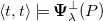 $\langle t,t \rangle \models {\boldsymbol{\Psi }}^\bot _{\lambda }({P})$
. With this we can apply Lemma18 to get that
 $\mathbf{M}\models {P}$
.
We then prove that it is in equilibrium. By construction
 $\mathbf{M}$
is total. We assume towards a contradiction that there is
 $\mathbf{M}'=(\langle \mathbf{H},\mathbf{T} \rangle ,{\tau })$
such that
 $\mathbf{H}\lt \mathbf{T}$
and
 $\mathbf{M}'\models {P}$
Then, there is
 $a\in \mathcal{A}$
such that
 $a\in T_k$
and
 $a\not \in H_k$
, for some
 $0 \leq k \lt \lambda$
. We apply Lemma17, and let
 $\langle h,t \rangle$
be the
 $\textrm {HT}_{\!c}$
interpretation such that
 $\langle h,t \rangle \models {\boldsymbol{\Pi }}_\lambda ({P})\cup \Delta ^c_{\lambda }\cup {\boldsymbol{\Psi }}^c_{\lambda }({P})$
with
 $\nu ={\tau }(\lambda -1)$
, and
 $\langle H,T \rangle |_{\mathcal{A}^{*}\cup {{\mathcal{T}}^c}}=\theta (\mathbf{M}')$
. By construction
 $(a_k,\boldsymbol{t})\in t$
and
 $(a_k,\boldsymbol{t})\not \in h$
, which means that
 $\langle h,t \rangle \lt \langle t,t \rangle$
leading to a contradiction since
 $\langle t,t \rangle$
is a constraint equilibrium model. Since there is no smaller model,
 $\mathbf{M}$
is in equilibrium.





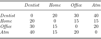
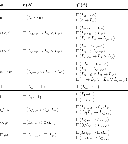
 η(ϕ)
 η∗(ϕ)
 ϕ
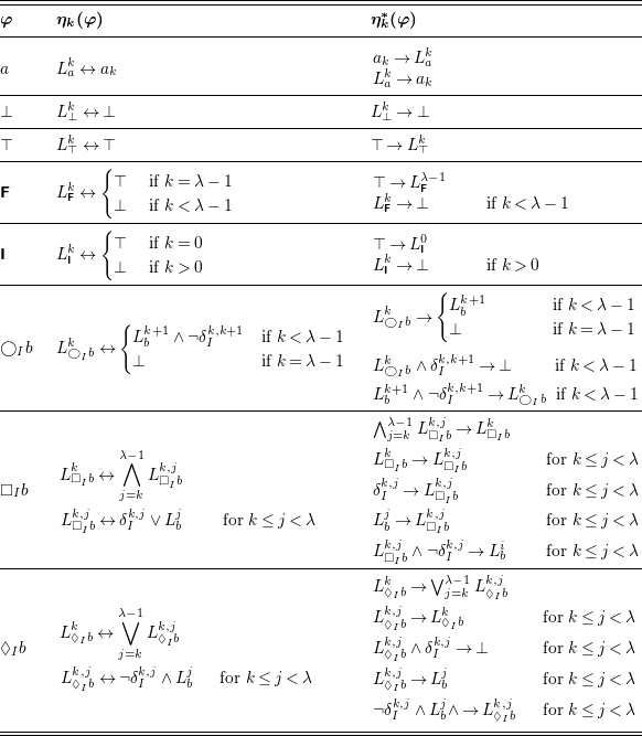
 ηk(φ)
 ηk∗(φ)
 φ
 0≤k<λ
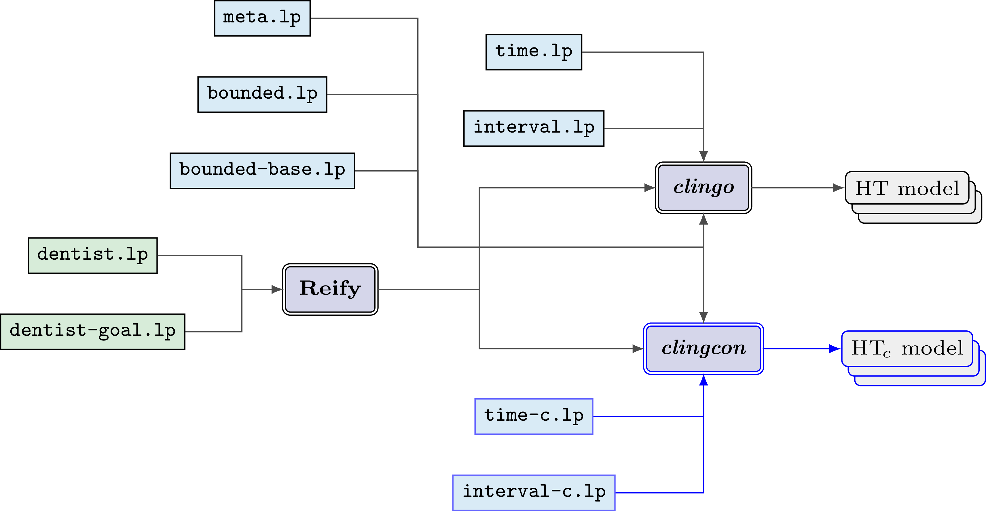
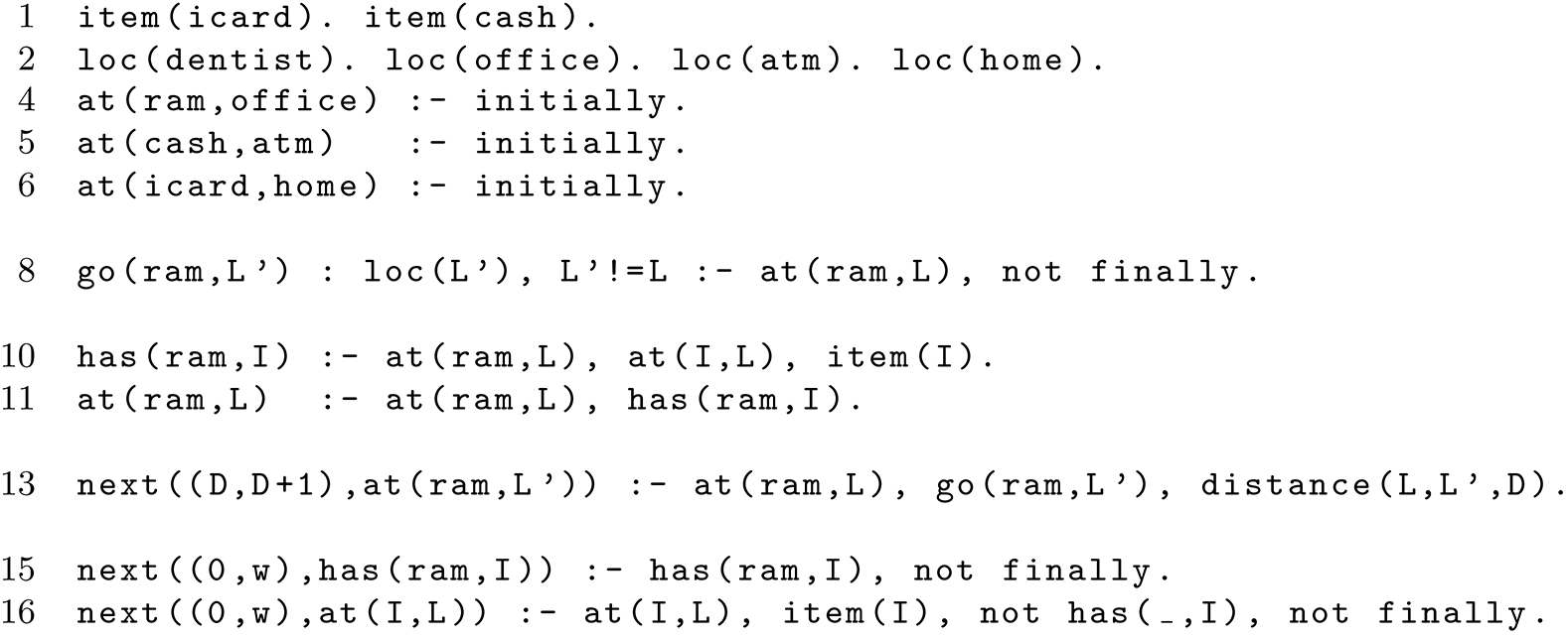

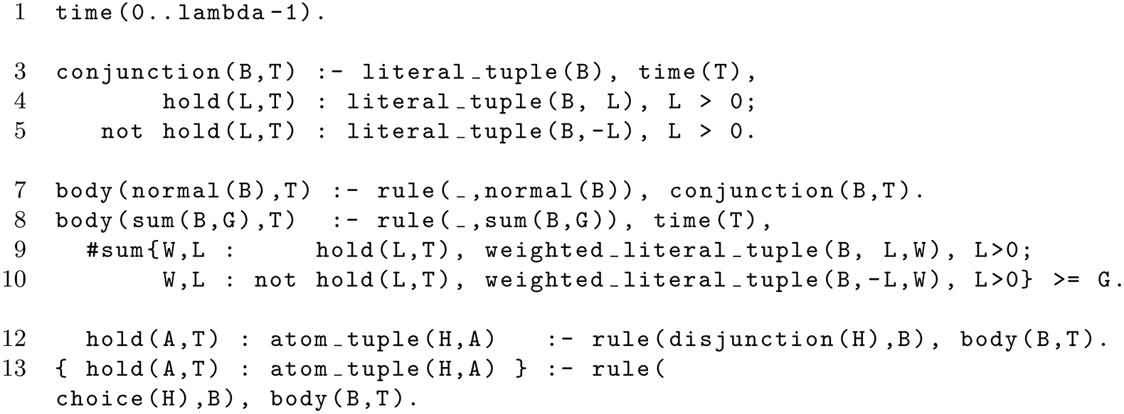
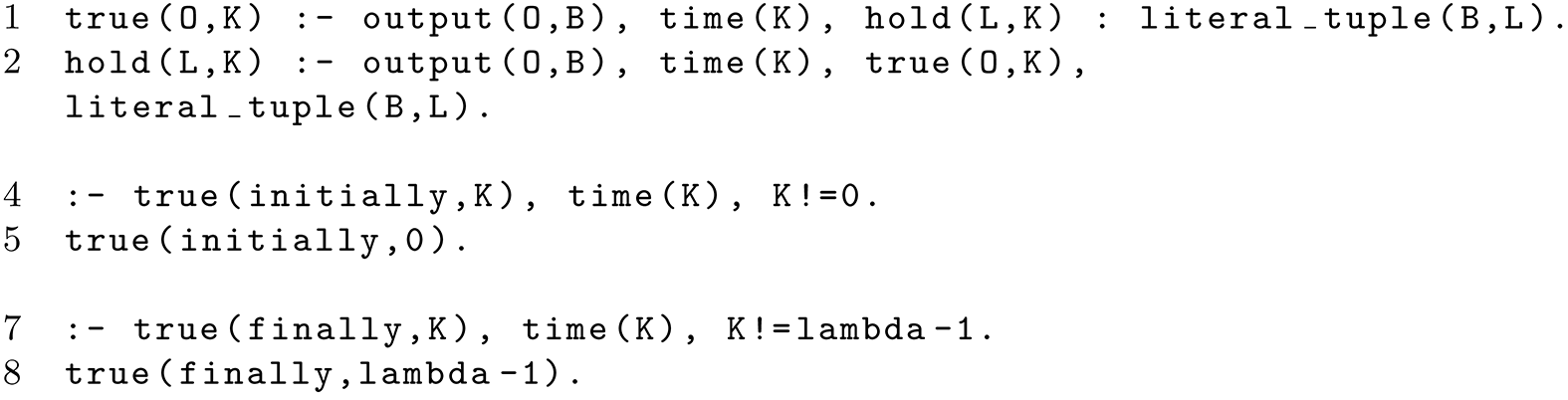

 Πλ(P)

 Δλ,ν

 Ψλ,ν(P)

 Δλc

 Ψλc(P)
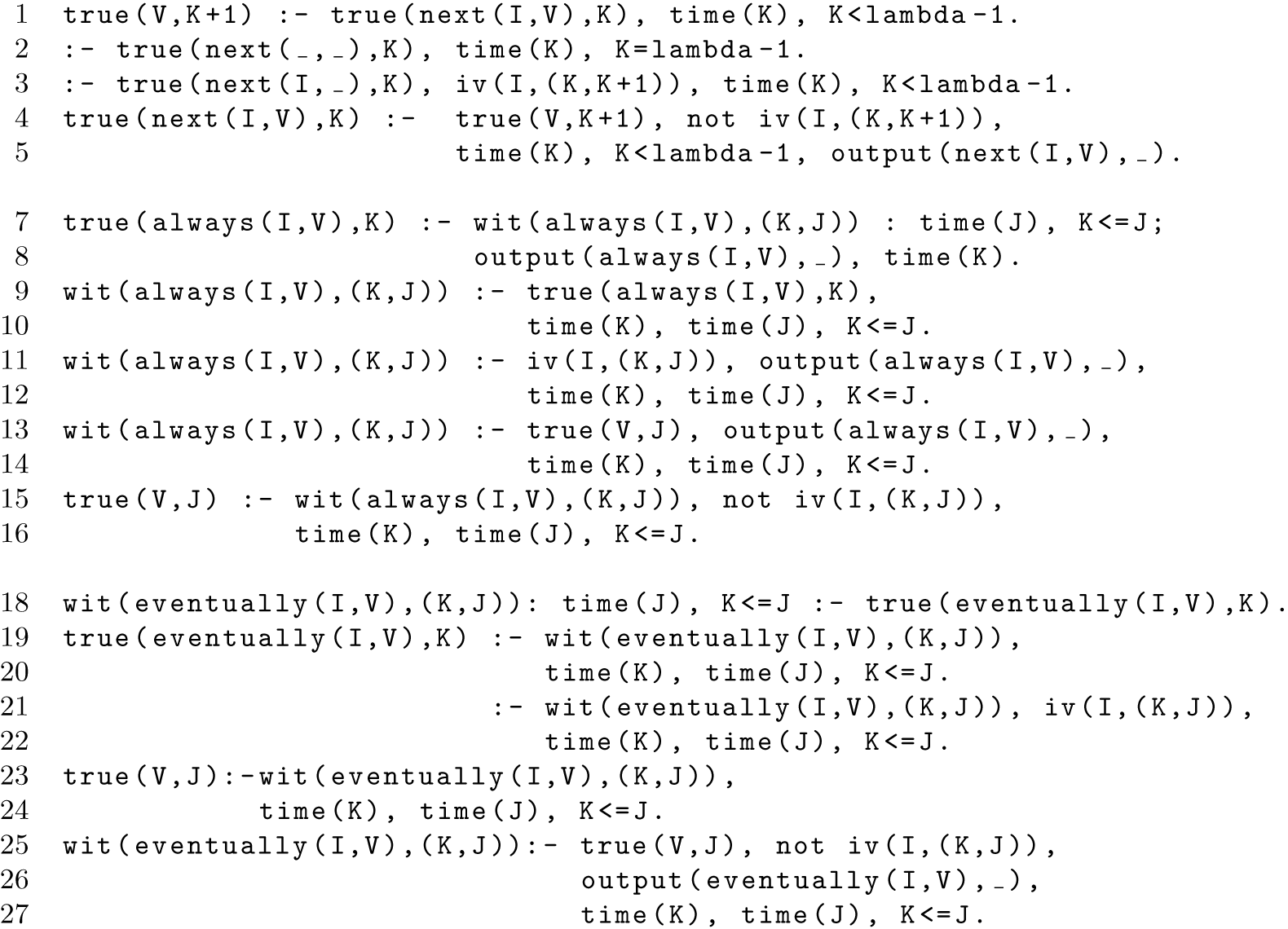
 Πλ(P)

 Ψλ,ν(P)

 Ψλc(P)
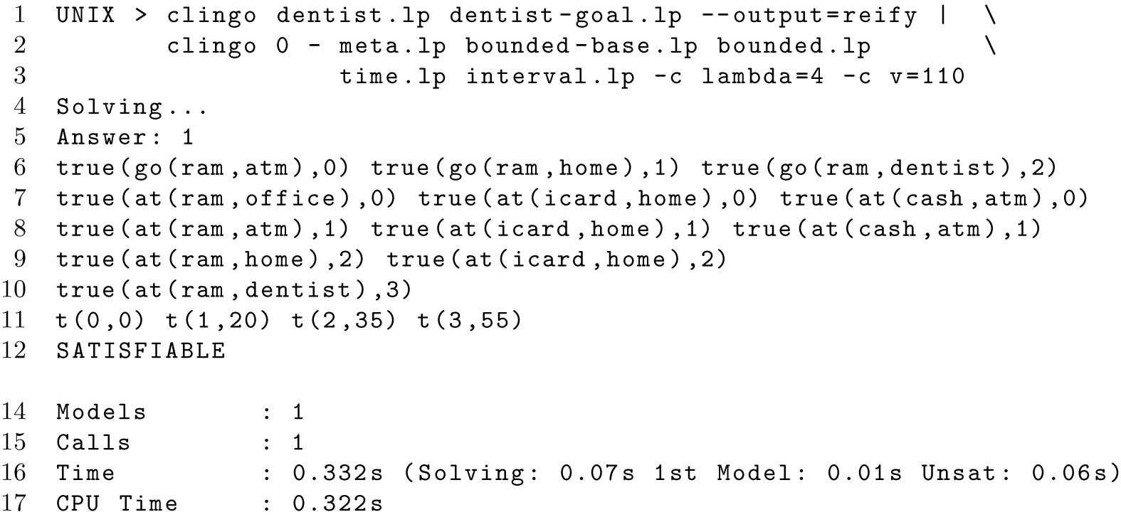
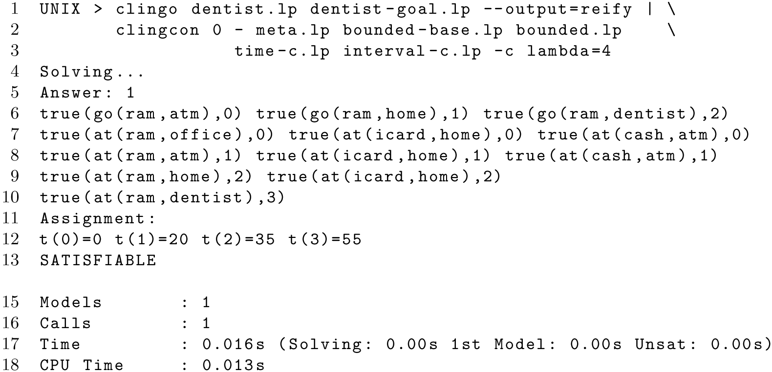
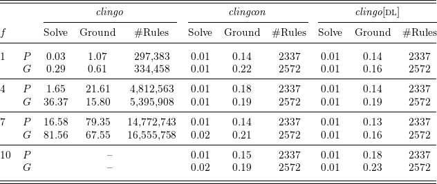
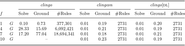
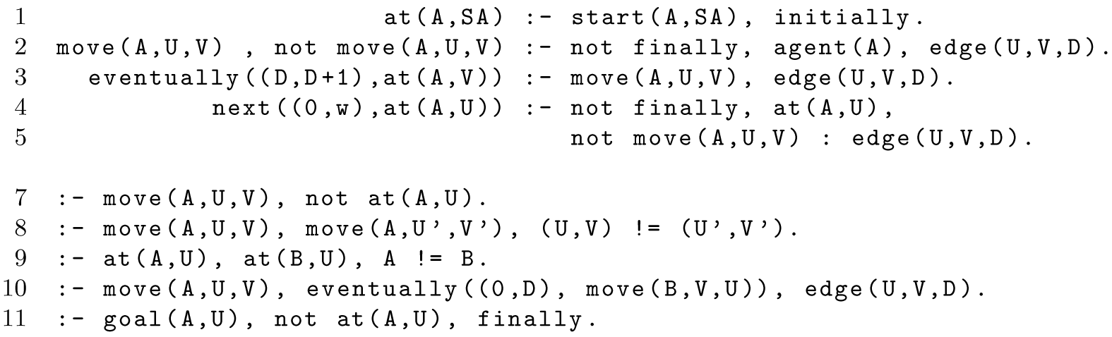
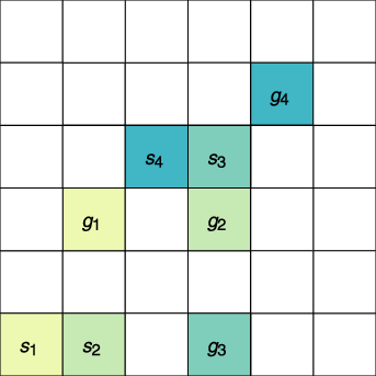
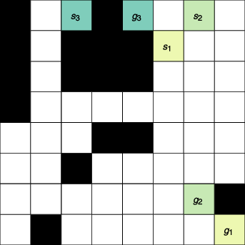
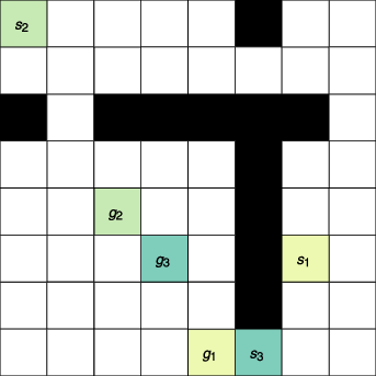
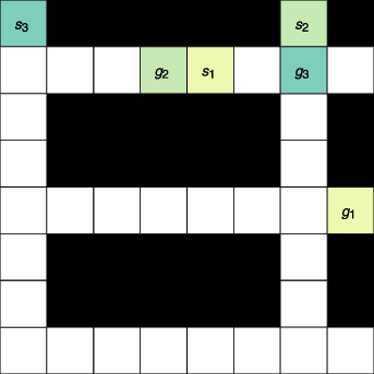
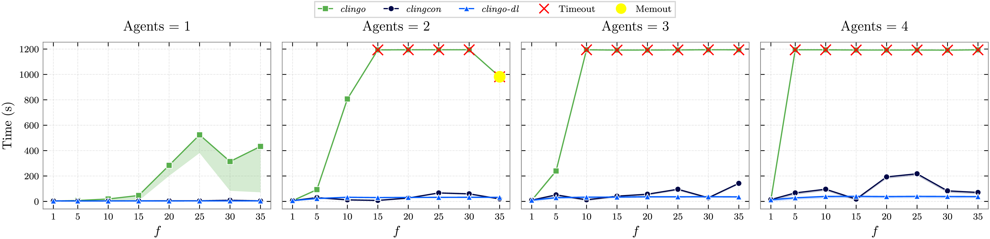
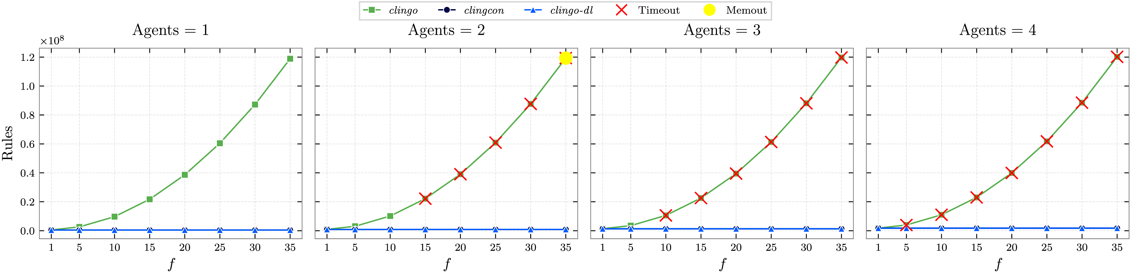

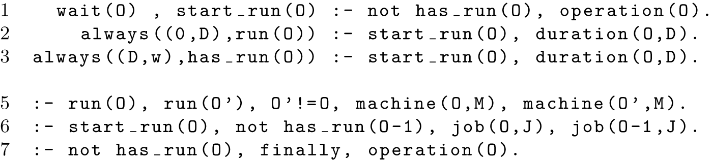
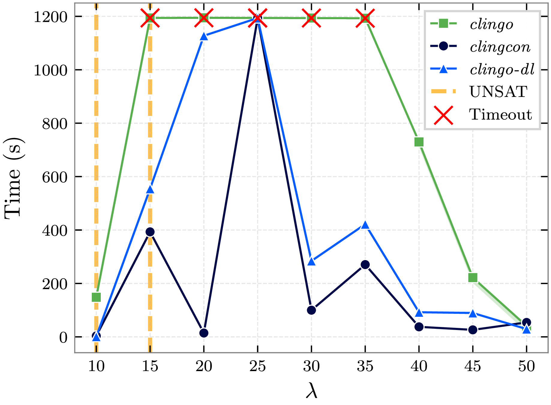
 ν=55
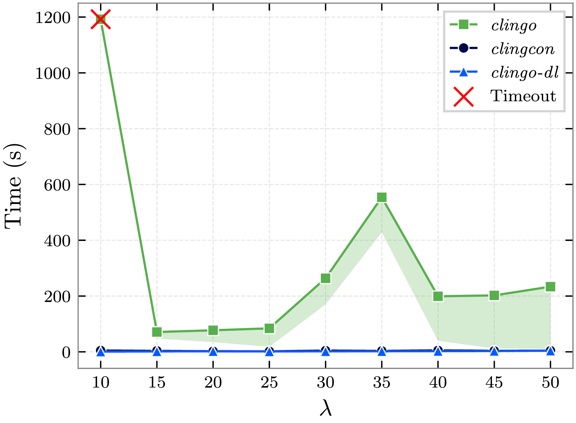
 ν=110
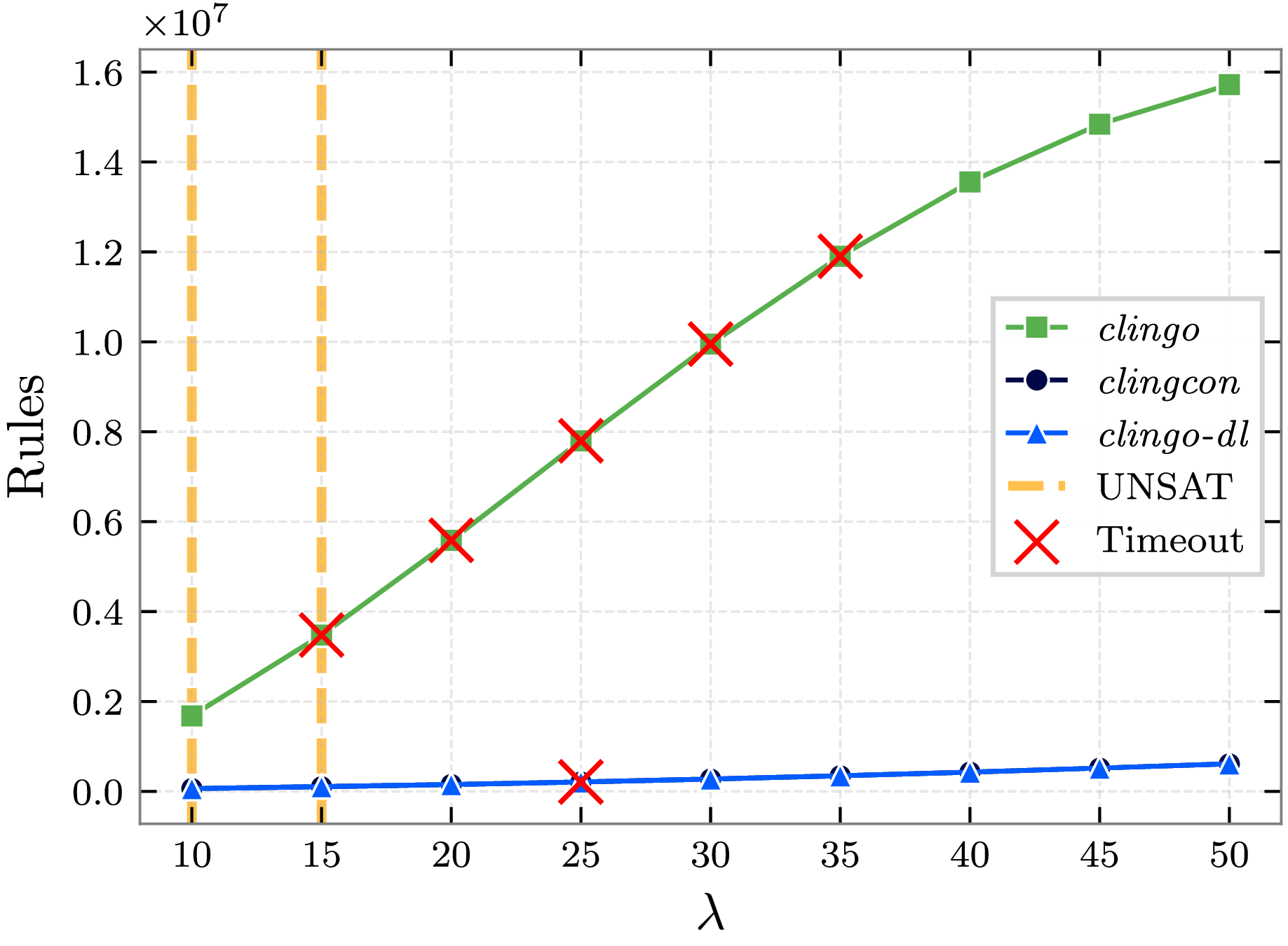
 ν=55
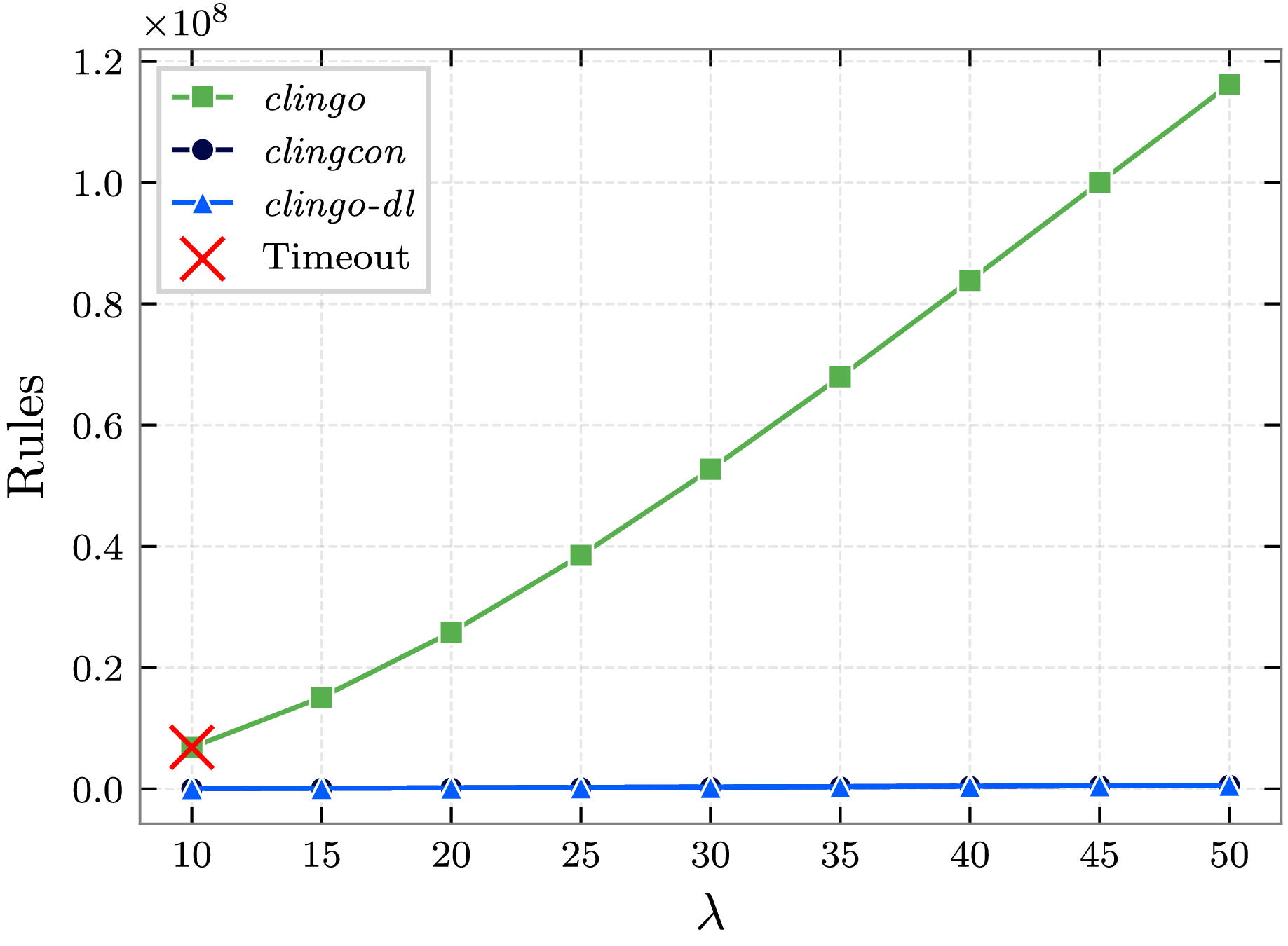
 ν=110
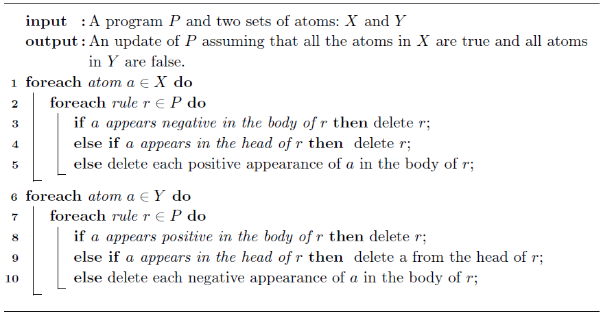

 Open access

