1. Introduction
A fundamental problem of dissipation of flows in collisionless plasmas moving faster than all plasma modes available has numerous laboratory, astrophysical and geophysical applications. It was realized more than half a century ago (for reviews, see e.g. Sagdeev Reference Sagdeev1966; Kennel, Edmiston & Hada Reference Kennel, Edmiston and Hada1985; Papadopoulos Reference Papadopoulos1985) that, despite lacking collisions, a shock wave must form in such flows. The new applications now pose new challenges to our understanding of collisionless shock structure and their potential to accelerate particles (Blandford & Eichler Reference Blandford and Eichler1987; Malkov & Drury Reference Malkov and Drury2001; Bulanov et al. Reference Bulanov, Esirkepov, Khoroshkov, Kuznetsov and Pegoraro2002; Adriani et al. Reference Adriani, Barbarino, Bazilevskaya, Bellotti, Boezio, Bogomolov, Bonechi, Bongi, Bonvicini, Borisov, Bottai, Bruno, Cafagna, Campana, Carbone, Carlson, Casolino, Castellini, Consiglio, De Pascale, De Santis, De Simone, Di Felice, Galper, Gillard, Grishantseva, Jerse, Karelin, Koldashov, Krutkov, Kvashnin, Leonov, Malakhov, Malvezzi, Marcelli, Mayorov, Menn, Mikhailov, Mocchiutti, Monaco, Mori, Nikonov, Osteria, Palma, Papini, Pearce, Picozza, Pizzolotto, Ricci, Ricciarini, Rossetto, Sarkar, Simon, Sparvoli, Spillantini, Stozhkov, Vacchi, Vannuccini, Vasilyev, Voronov, Yurkin, Wu, Zampa, Zampa and Zverev2011; Haberberger et al. Reference Haberberger, Tochitsky, Fiuza, Gong, Fonseca, Silva, Mori and Joshi2012; Fiuza et al. Reference Fiuza, Stockem, Boella, Fonseca, Silva, Haberberger, Tochitsky, Mori and Joshi2013; Blandford, Simeon & Yuan Reference Blandford, Simeon and Yuan2014). Microscopically, strong shocks can be supported by suitable plasma waves that randomize particle trajectories in lieu of binary collisions. Although these waves are not necessarily energetically important (i.e. contribute to the Rankine–Hugoniot relation, radiate part of the shock energy, etc.), in many cases they are driven by shock-reflected particles. In this paper we consider relatively weak shocks in which the crucial process of ion reflection can be effectively approached from the well-understood physics of solitary waves.
The shock at first results from a nonlinear steepening of a certain mode whose dispersion often limits the steepening. For a number of modes, nonlinearity and dispersion can balance each other exactly, which results in a soliton. In this paper we consider the most fundamental ion-acoustic solitons with a trailing wave train (Moiseev & Sagdeev Reference Moiseev and Sagdeev1963; Sagdeev Reference Sagdeev1966), which are the building blocks of collisionless shock waves in non-isothermal plasmas, with the electron temperature much higher than the ion temperature,
 $T_{e}\gg T_{i}$
. Our study is relevant to electrostatic shock propagation in laser-produced plasmas (Mourou, Tajima & Bulanov Reference Mourou, Tajima and Bulanov2006; Sorasio et al.
Reference Sorasio, Marti, Fonseca and Silva2006; Romagnani et al.
Reference Romagnani, Bulanov, Borghesi, Audebert, Gauthier, Löwenbrück, Mackinnon, Patel, Pretzler, Toncian and Willi2008; Palmer et al.
Reference Palmer, Dover, Pogorelsky, Babzien, Dudnikova, Ispiriyan, Polyanskiy, Schreiber, Shkolnikov, Yakimenko and Najmudin2011; Fiuza et al.
Reference Fiuza, Stockem, Boella, Fonseca, Silva, Haberberger, Tochitsky, Mori and Joshi2013; Macchi, Borghesi & Passoni Reference Macchi, Borghesi and Passoni2013), especially to the generation of monoenergetic ion beams and to shock-related processes in astrophysical and space plasmas. Among the astrophysical and geophysical applications of this study, we would like to mention ion injection into the first-order Fermi acceleration in astrophysical shocks. The injection process is crucial for the resolution of problems such as the origin of cosmic rays. Overall, the cosmic-ray spectrum is a power law starting from suprathermal energies. The injection ensures a smooth transition between the thermal plasma and the power-law spectrum at high energies. Although the power-law component is due to multiple shock front crossings, and not so much due to the reflection from the shock, particle reflection can also contribute to the high-energy part of the spectrum, if the shock is oblique. In this case the magnetic field is important. The electrostatic mechanism is not efficient at high particle energies. However, our purely electrostatic simulations are relevant to the microphysics of particle reflection off the shock front, including cosmic-ray-loaded shocks.
2. Model and simulation set-up
In order to address the ions that are reflected from and escape the shock, to incorporate the ion reflection into the global shock structure and to investigate its effect on the shock itself, we use the kinetic plasma description. The plasma dynamics is governed by the Vlasov equations for the distribution functions of the plasma components and the Poisson equation for the electrostatic field. Numerically, we solve the Vlasov equations using the particle-in-cell (PIC) method (Dawson Reference Dawson1983), and the electrostatic field is obtained by direct integration of the charge density, which in turn is calculated from the individual particle positions. For the solution of the equations of motion of particles, an organic time-reversible and second order in time leapfrog algorithm is applied. The second-order accuracy in space is obtained by calculating the electric field and the charge density on staggered grids.
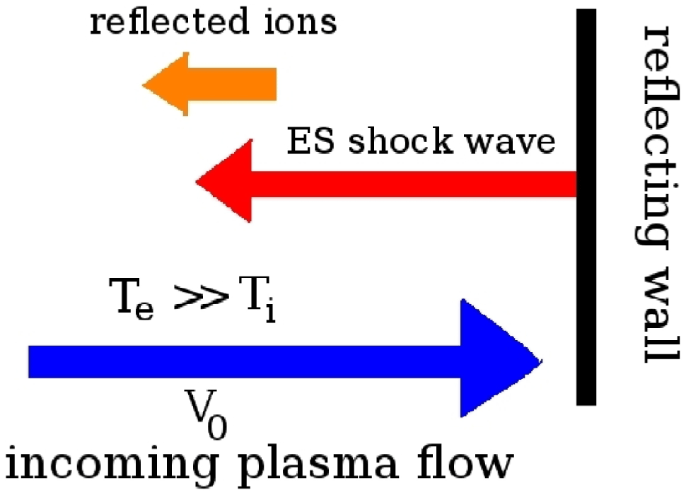
Figure 1 shows the schematic set-up for our one-dimensional (1D) simulations. A shock wave is produced by reflection of a high-speed electron–ion plasma off a conducting wall. The shock forms due to the interaction between the incoming and reflected flows and propagates away from the wall. We measure the density of fully ionized hydrogen plasma components in units of the unperturbed density
 $n_{0}$
, coordinates in units of the Debye length of the unperturbed plasma flow
 ${\it\lambda}_{D}=\sqrt{T_{e}/4{\rm\pi}e^{2}n_{0}},$
velocity in units of the electron thermal speed
 $v_{Te}=\sqrt{T_{e}/m_{e}}$
, and time and electric field in units of
 $1/{\it\omega}_{pe}=\sqrt{m_{e}/4{\rm\pi}e^{2}n_{0}}$
and
 $E_{0}=\sqrt{4{\rm\pi}n_{0}T_{e}}$
, respectively. In the PIC simulations, we ensure high enough resolution to resolve low-density regions, sharp gradients and the dynamics of both electrons and ions by taking at least 100 particles per cell and a spatial resolution better than
 $0.05{\it\lambda}_{D}$
. For reference, in all simulations shown, the conducting wall is located at
 $x=0$
and the plasma flow impinges on it at
 $t=0$
. Within these settings, the dimensionless input parameter that determines the evolution of the plasma flows is
 $M_{0}=V_{0}/C_{s}$
, where
 $V_{0}$
is the speed of unperturbed plasma flow and
 $C_{s}=\sqrt{T_{e}/m_{i}}$
is the sound speed. Moreover, the stability of the soliton and the formation of the shock are proven to be strongly dependent on the velocity distribution of ions (Macchi, Nindrayog & Pegoraro Reference Macchi, Nindrayog and Pegoraro2012), thus on the fraction
 $T_{i}/T_{e}$
.
Scheme of the set-up for 1D kinetic modelling of electrostatic shock wave.

Note that this purely electrostatic approach is reasonable for quasi-parallel shocks, as it treats scales
 ${\it\lambda}_{D}<l<c/{\it\omega}_{pi}\sim r_{g}^{i}$
(as
 ${\it\beta}\sim 1$
very often), thus providing an important microphysics ingredient for the diffusive shock acceleration as well (Drury Reference Drury1983, Reference Drury2012; Bell Reference Bell2014). Here
 ${\it\omega}_{pi},r_{g}^{i}$
and
 ${\it\beta}$
are the ion plasma frequency, ion gyroradius and thermal/magnetic energy ratio, respectively. The hybrid simulations, broadly used in astro-geo-shock studies, do not resolve these scales since they treat electrons as a fluid.
3. Simulation results
3.1. Cold upstream ions
The evolution of the distribution of ions on the phase plane
 $(x,V_{x})$
for
 $M_{0}=V_{0}/C_{s}=1.3$
is shown in figure 2(a–d). By
 $t=200{\it\omega}_{pe}^{-1}$
the flows have interacted and the shock is formed. The isolated density (and electrostatic potential) structures, figure 2(e, f), have a characteristic width of several
 ${\it\lambda}_{D}$
. Ions reflected from the shock are clearly visible on the phase plane. The first outrunning ions are produced by the reflection from the wall. In the case of cold upstream ions, the ions are reflected at a single point where the potential reaches its maximum and the electric field has a jump and the potential profile a cusp.
(a–d) Distribution of the ions on the
 $(x,V_{x})$
phase plane; (e, f) distributions of the electrostatic potential and ion density at
 $t{\it\omega}_{pe}=880,~1520,~2160,~2800$
for
 $M_{0}=V_{0}/C_{s}=1.3$
. The colours correspond to the number of ions with respect to the number of inflowing ions (per unit length) in logarithmic scale according to the colour bar. The leading soliton has a cusp structure. It occurs only when the cold ions get reflected.

The number of ions reflected out of the shock increases with increasing flow velocity – see figure 3, where the distributions of ions on the phase plane
 $(X,V_{x})$
and the distribution functions of ions
 $f_{i}(v)$
at
 $t{\it\omega}_{pe}=2800$
are shown. The distribution function has three distinct peaks: inflowing ions (
 $v=V_{0}$
), reflected ions (
 $|v|\simeq V_{0}+2V_{front},$
with
 $V_{front}$
the speed of the reflecting hump), and ions at rest downstream of the shock. The energy spectrum of the reflected ions is very broad. The number of shock-reflected ions for
 $M_{0}=3$
is approximately 40 times bigger than for
 $M_{0}=1.3$
and 3.5 times bigger than for
 $M_{0}=2.1$
.
(a–d) Distribution of ions on the
 $(X,V_{x})$
phase plane for different values of
 $M_{0}=V_{0}/C_{s}$
. The colours correspond to the number of ions with respect to the number of inflowing ions (per unit length) in logarithmic scale according to the colour bar. Only the particles inside outlined by the black ellipses were reflected out from the conducting wall. (e) Distribution function of ions
 $f_{i}(v)$
at
 $t{\it\omega}_{pe}=2800$
.

The spatial distributions of the electrostatic potential (
 $-e{\it\phi}$
) for different values of upstream flow are presented in figure 4(a,b). It is clearly seen that, when the ions begin to reflect from the soliton tip, the classical single solution bifurcates into a more complex structure that comprises the leading soliton, the periodic wave train downstream of it and the foot occupied by the reflected ions. This foot is supported by the reflected ions and also accelerates them somewhat further. Because of the reflection of cold ions, the leading soliton for
 $M_{0}=1.3$
, 2.1 and 3 acquires a clear cusp structure.
(a,b) Distribution of the electrostatic potential for
 $M_{0}=0.4,~1.3,~2.1,~3$
at
 $t{\it\omega}_{pe}=1400$
and
 $t{\it\omega}_{pe}=2800$
. (c) Evolution of the maximum of the electrostatic potential
 $-e{\it\phi}_{max}$
(solid line) and of the position of the shock front
 $X_{max}$
(dashed line). (d) The velocity of the shock. The cusp structure in the potential occurs if cold ions are reflected. The outer soliton is liberated from its dispersive tail. The solution is asymmetric with respect to the reflection point, and downstream it is oscillatory. Upstream of the soliton, reflected ions create a foot with an elevated electrostatic potential.

The particle reflection strongly depends on the amplitude of the shock (overshoot of electrostatic potential), the amplitude of which depends on the shock speed (Moiseev & Sagdeev Reference Moiseev and Sagdeev1963; Sagdeev Reference Sagdeev1966; Gurevich Reference Gurevich1968) in the first place. In turn, it alters the shock amplitude and speed, and thus the reflection threshold. Moreover, the reflected ions perturb the electrostatic potential upstream, which changes the speed of inflowing ions and thus, again, the condition for the ensuing reflection. For
 $M_{0}=2.1$
and
 $3$
the shock loses much of its momentum because of ion reflection; for
 $M_{0}=1.3$
the number of reflected ions is very small. Momentum conservation suggests that ion reflection slows down the shock, thus decreasing its amplitude. Evidently, decreasing amplitude acts against reflection. However, if the amplitude drops below the reflection threshold for a given speed, the shock amplitude should recover and the reflection will resume. By virtue of these feedback loops, the reflection efficiency can be expected either to stay at a self-organized critical level or to exhibit cyclic dynamics. Numerical simulations and observations validate both scenarios, though the cyclic shock behaviour was primarily observed in magnetized plasma environments (Burgess, Möbius & Scholer Reference Burgess, Möbius and Scholer2012; Caprioli, Pop & Spitkovsky Reference Caprioli, Pop and Spitkovsky2015). The temporal evolution of the maximum value (
 $-e{\it\phi}_{max}$
) of the electrostatic potential extracted from our simulations, figure 4(c) (solid line), confirms the cyclic behaviour of the shock.
The approximate velocity of the shock with respect to the upstream flow can be defined from the position of the maximum of the electrostatic potential (dashed curves in figure 4
c) and is shown in figure 4(d). Measured in units of
 $C_{s}$
, this velocity directly represents the shock Mach number
 $M_{A}=V_{shock}/C_{s}$
. Our simulations show that the solution, consisting of the leading soliton, periodic wave train downstream and the foot occupied by the reflected ions, persists with increasing Mach numbers up to a critical value of
 $M_{A}=M_{2}\simeq 4.5$
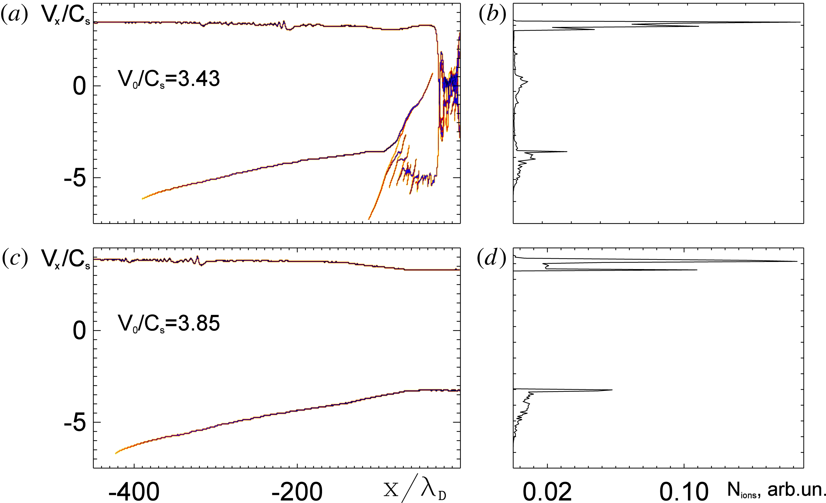
at which almost all incident ions get reflected. In the case of cold ions, this critical value is reached for the upstream velocity
 $V_{0}=V_{2}=3.43C_{s}$
. The obtained critical value of
 $M_{2}$
is much beyond the critical value
 $M_{\star }$
, at which the shock is about to reflect some of the upstream ions. For the cold upstream ions and Bolzmannian electrons (this is definitely not the case in our simulations),
 $M_{\star }\simeq 1.6$
(Sagdeev Reference Sagdeev1966), for adiabatically trapped electrons
 $M_{\star }\simeq 3.1$
(Gurevich Reference Gurevich1968). Note that, in the early days of collisionless shock research, the existence of stationary shock transitions for Mach numbers exceeding the critical
 $M_{\star }$
has been often disfavoured. Note also that, when the velocity of the incoming flow is greater than
 $V_{2}$
, the solution becomes qualitatively very different. An example is given in figure 5, where a beam of ions produced by the reflection of the inflowing ions with
 $M_{0}=3.85$
out of the conducting wall is clearly seen. Note also the sharp peak in the distribution function (
 $v_{i}<0$
) and the significant deceleration of the inflowing ions (
 $v_{i}>0$
) for
 $M_{0}=3.85$
. The next qualitative change in the solution should occur when the inflow velocity reaches values comparable to the thermal velocity of the electrons. At this point the Buneman instability starts to play an important role in the interaction of flows. This regime however is outside the current study.
Distribution of ions on
 $(X,V_{x})$
phase plane (a,c) and distribution function of ions
 $f_{i}(v_{i})$
(b,d) at
 $t{\it\omega}_{pe}=2800$
for
 $M_{0}=3.43$
and
 $M_{0}=3.85$
. For
 $M_{0}=3.85$
the flow velocity of the incident plasma exceeds the critical value
 $V_{2}$
.

Finally, figure 6 shows the distribution of ion density
 $n_{i}(x,t)$
in logarithmic scale and the time history
 $x_{i}(t)$
of some selected ions. The first peak in the ion density corresponds to the ‘outrunner’ soliton, liberated from its dispersive trail. The velocity of this soliton is almost constant in time (apart from the oscillations, mentioned above) and it reflects a lot of incoming ions, which then escape with double the shock speed. The trail, instead, not only propagates with a smaller velocity, but also slows down significantly as well. Some of the ions get trapped between the soliton and the leading part of the trail.
Ion density distribution and ion time history for
 $M_{0}=2.14$
.

3.2. Warm upstream ions
The resolution of our PIC simulations is high enough to accurately include the finite ion temperature in our analysis. Figure 7 shows the distributions of ions on the phase plane for
 $M_{0}=0.4$
(very slow upstream flow) and cold/warm upstream ions. If the upstream ions are cold (
 $T_{i}=0$
), only a negligibly small number of them get reflected; but if
 $T_{i}>0$
, the final distribution function of ions assumes a different shape. In figure 7 a steady reflection of ions is clearly visible for
 $T_{i}>0$
. Their number remains, however, very small and the energy spectrum remains quite broad. Moreover, there are ions trapped in the ‘multi-peaks’. Note that the stability of solitons and the formation of electrostatic shock waves in ultra-intense laser interaction with overdense plasmas (Macchi et al.
Reference Macchi, Nindrayog and Pegoraro2012) are also found to be strongly dependent on the velocity distribution of the ions. It should be mentioned that, if the flow velocity of warm (both electrons and ions) inflowing plasma exceeds
 $V_{2}$
, the solution qualitatively similar to figure 5 forms again: the reflection produces a huge amount of almost monoenergetic ions that propagate away from the shock.
Distribution of the ions on the
 $(X,V_{x})$
phase plane for
 $M_{0}=V_{0}/C_{s}=0.4$
and
 $T_{i}=0$
(a),
 $T_{i}=0.045T_{e}$
(b) and
 $T_{i}=0.09T_{e}$
(c). The colours correspond to the number of ions with respect to the number of inflowing ions (per unit length) in logarithmic scale according to the colour bar.

4. Conclusion
Our simulations show that (i) when the Mach number of the acoustic soliton increases to the point of ion reflection and the soliton transforms into a soliton and a trailing wave train downstream, this structure persists with increasing Mach number until almost all incident ions get reflected; (ii) the ion reflection alters the shock amplitude and speed, thus impacting the reflection threshold itself; and (iii) the pedestal of the electrostatic potential, supported by the reflected ions, changes the speed of inflowing ions and thus, again, the condition for the ensuing reflection. The formation of the pedestal in the potential between the reflecting hump and the front edge of the group of reflected ions makes the analytic theory very challenging. In fact, this pedestal is sensitive to the model used for the transition between the reflected ions and upstream (e.g. cold versus hot beam of reflected ions). In the pedestal the inflowing plasma is slowed down considerably if its front edge moves at the speed of the main shock, but reflected particles pass through it and accelerate, decreasing their density. All these uncertainties are critical and hard to resolve without simulations. Note that an analytic solution for the ion-acoustic collisionless shock with self-consistently reflected ions and their subsequent cooling was recently presented by Sagdeev et al. (Reference Sagdeev, Malkov, Diamond, Dudnikova, Liu and Su2013) and Malkov et al. (Reference Malkov, Sagdeev, Dudnikova, Liseykina, Diamond, Liu and Su2014). Its relation to the well-known non-reflecting ion-acoustic soliton solution, strictly limited by the critical Mach number
 $M_{\star }=1.6$
(Boltzmann electrons) and
 $M_{\star }=3.1$
(trapped electrons), is clarified and quantified.
Acknowledgements
This work was in part supported by the DFG within the SFB 652 and by RSCF within 14-11-00485. PIC simulations were performed using the computing resources granted by the John von Neumann-Institut for Computing (Research Center Jülich) under the project HRO03.