





Nomenclature
- ATM
-
air traffic management
- ATCOs
-
air traffic controllers
- ATFM
-
air traffic flow management
- CB
-
cumulonimbus
- GS
-
ground speed
- MILP
-
mixed-integer linear programming
- MINLP
-
mixed-integer nonlinear programming
- NLP
-
nonlinear programming
- NMPC
-
nonlinear model predictive control
- RHC
-
rolling horizon control
- TAS
-
true airspeed
- TMA
-
terminal manoeuvring area
- TP
-
test problem
- TS
-
thunderstorm
- VSS
-
value of the stochastic solution
1. Introduction
1.1. Motivation
Trajectory optimisation aims to obtain cost-efficient flights and enhance overall operational efficiency. Therefore, it is a fundamental aspect of the air traffic management (ATM) system. However, convective weather areas significantly affect aircraft operations and create major challenges for aircraft trajectory planning in ATM systems. In these areas, severe weather events such as hail, wind shear, lightning, severe icing and turbulence present major safety risks to aircraft. For this reason, aircraft should avoid them to minimise the risk of encountering severe weather events. Hence, an effective flight trajectory planning algorithm is crucial in ATM, as it can help aircraft avoid these events.
Avoiding convective weather leads to deviations from planned flight plans, which cause air traffic disruptions when multiple flights are affected simultaneously. Such disruptions will increase flight time and delay, resulting in congestion and additional fuel consumption within the airspace [Reference Kaplan, Çetek and Saraç1]. Delays occur due to convective weather, which introduces challenges in predicting air traffic and adds complexity to its management. Additionally, the workload of the flight crew increases significantly due to decision-making, turbulence, icing management and increased communications. Similarly, air traffic controllers (ATCOs) experience a substantial workload increase during convective weather, mainly due to irregular air traffic and less available airspace. These factors reduce the airspace capacity, consequently negatively affecting flight efficiency. Furthermore, the inherent uncertainty of convective weather and its impact on airspace capacity require advanced safety measures and automated flight routeing systems.
Convective weather conditions remain a major contributor to delays in European air traffic flow management (ATFM). Approximately 4 million minutes of delay per year are attributed to convective weather conditions during en-route flights [2]. In July 2023, Europe experienced convective weather conditions, including thunderstorms. EUROCONTROL reported that the weather-related ATFM delay for this month exceeded two and a half times that of the previous year. When excluding weather-related factors, ATFM delays per flight decreased by almost a quarter despite a 7% increase in air traffic. However, when considering the impact of convective weather, delays increased slightly from 3.9 to 4.1 min per flight [3]. This indicates that convective weather contributes to air traffic delays, highlighting the need for improved strategies to mitigate its operational impact and enhance flight efficiency. Therefore, EUROCONTROL initiated the SMART Weather Task Force programme to enable collaborative management of convective weather conditions [4].
Convective weather events are also impacted by climate change. As global temperatures rise, changes in atmospheric conditions influence convective weather phenomena like thunderstorms, tornadoes and heavy rainfall. However, it is important to note that these effects can vary depending on regional and local atmospheric conditions. Some studies and researchers have examined the impact of global warming on weather phenomena, including thunderstorms, and have noted that some regions may experience frequent and intense convective weather events while others may see different climate changes [Reference Allen5–Reference Raupach, Martius, Allen, Kunz, Lasher-Trapp, Mohr, Rasmussen, Trapp and Zhang8].
In addition to the challenge of avoiding convective weather conditions, potential conflicts between aircraft within the airspace represent another critical operational challenge. When pilots encounter convective weather along planned flight trajectories, they promptly notify ATCOs to determine the appropriate avoidance manoeuvres using weather radar. Multiple pilots within the same airspace may make similar requests, leading to potential conflicts as aircraft deviate from their flight trajectories. ATCOs are responsible for resolving these potential conflicts and providing necessary instructions to maintain safe air traffic flow by ensuring conflict-free flight trajectories. However, there is less available area in the airspace to resolve conflicts due to convective weather conditions, adding an extra complexity to ATM with irregular air traffic and increasing congestion. As airspace congestion continues to rise, the workload of ATCOs increases significantly. To address this, developing algorithms that propose conflict-free trajectories under convective weather conditions is essential. Decision support and/or automation systems based on these algorithms can be effective tools for improving the accuracy and efficiency of aircraft trajectory planning and coordination within the airspace. As a result, the use of these algorithms can help reduce ATCO workload, with potential benefits for operational safety and ATM capacity.
Some avoidance guidelines have been presented by authorities that describe what pilots should do to continue their flights safely in case of encountering convective areas [9–12]. However, Reference [Reference Trier and Sharman13] has shown that these guidelines are inadequate and overly simplify the hazardous turbulence conditions surrounding convective areas. Because the decision-making processes of pilots regarding weather conditions are highly complex and dynamic, pilots make decisions based on their own experience and real-time observations of weather information, along with information obtained from remotely sensed data and observed flight trajectories [Reference Rubnich and Delaura14]. Moreover, although some meteorological conditions can be predicted in advance, it is difficult to determine the specific location and time of convective weather. Therefore, convective weather forecasting and avoidance primarily occur during the flight at short timescales. The approach proposed in our study can guide pilots and ATCOs based on real-time observations through onboard weather radar of convective areas, along with indicators.
This study develops mathematical models to optimise aircraft trajectories in ATMs under convective weather conditions, specifically focusing on the dual challenges of avoiding convective areas and resolving conflicts between aircraft during en-route flights. This approach not only contributes to the theoretical foundation but also addresses practical applications in enhancing flight safety and efficiency. To achieve this, we have proposed two distinct models, one utilising a deterministic approach and the other employing stochastic programming that considers the uncertainties of both wind direction and speed. The objective of these models is to minimise the total flight time of the aircraft while determining flight trajectories between the entry and exit points of the airspace under convective weather conditions. Moreover, we have implemented a rolling horizon control (RHC) approach to address the dynamic nature of convective areas. This framework allows us to address changes in the size and displacement of the convective areas over time, including merging, splitting, dissipating and growing behaviour, thereby enhancing the effectiveness of models in optimising flight paths.
1.2. Literature review
There are studies in the literature that detect and resolve potential conflicts between aircraft during the en-route phase of flights. These studies aimed to explore effective conflict resolution techniques, manoeuvre strategies and solution approaches to ensure the safe and efficient management of airspace. Researchers have introduced several mathematical models, including mixed-integer linear programming (MILP) and mixed-integer nonlinear programming (MINLP), as well as heuristic and metaheuristic algorithms. These models and algorithms utilise airspace discretisation and geometric structure-based discretisation techniques to deal with conflict resolution.
Cecen and Cetek [Reference Cecen and Cetek15] resolved potential conflicts between aircraft using entry point assignment and speed change manoeuvres, while in another study Reference [Reference Cecen and Cetek16], employed entry point assignment and heading change manoeuvres for conflict resolution. Additionally, Reference [Reference Cecen, Saraç and Cetek17] addressed conflicts involving changes in heading and altitude. In all three studies, the authors utilised the airspace discretisation technique and assumed conflict resolution manoeuvres would take place within a predefined buffer zone within the boundaries of the airspace. Together with the mathematical model, they proposed using heuristic and metaheuristic algorithms for the problem solution, including simulated annealing and tabu search. Some researchers [Reference Cafieri and Durand18–Reference Vela, Solak, Singhose and Clarke21] have also used the airspace discretisation technique to resolve conflicts without defining any buffer zone within the airspace. These studies have introduced a mathematical model, with the first study by Reference [Reference Cafieri and Durand18] also proposing a heuristic algorithm.
In addition to the studies mentioned above, several studies have been conducted on mathematical models based on the geometric structure approach. In the study by Reference [Reference Alonso-Ayuso, Escudero and Martín-Campo22], only the speed change manoeuvre was used to resolve conflicts between aircraft, while in the study by Reference [Reference Alonso-Ayuso, Escudero and Martín-Campo23], only the heading change manoeuvre was used. However, in some studies [Reference Cafieri and Omheni24–Reference Vela, Solak, Clarke, Singhose, Barnes and Johnson27], both heading and speed change manoeuvres were used. Additionally, studies [Reference Alonso-Ayuso, Escudero and Martín-Campo28, Reference Alonso-Ayuso, Escudero, Olaso and Pizarro29] were conducted using both altitude and speed change manoeuvres. All three manoeuvres were used in the study [Reference Alonso-Ayuso, Escudero and Martín-Campo30]. On the other hand, solutions were produced using the heuristic algorithm [Reference Erzberger and Heere31] and the particle swarm optimisation metaheuristic algorithm [Reference Hong, Choi, Oh, Lee and Kim32]. In the first study, only heading change was used, while in the second study, both heading and speed change manoeuvres were used. The number of nodes used to discretise the airspace affects the solution time and quality of the model. A higher number of nodes leads to better solutions, but it also increases the solution time in both airspace discretisation and geometric structure-based approaches. Reference [Reference Kaplan, Çetek and Saraç33] presented a mathematical model to solve conflicts between aircraft. In their study, the airspace was discretised into low, medium and high node numbers to examine the effect of the discretisation rate on the solution time and quality.
Recent studies on aircraft trajectory optimisation have explored diverse methodological approaches to address operational, environmental and uncertainty-related challenges in ATM. Several studies have developed robust frameworks to consider weather-related uncertainties in trajectory planning. NG (2022) [Reference NG34] developed a robust flight path planning approach that accounts for fuel and contrail costs under meteorological uncertainty. The method models airspace as a directed graph, identifying contrail-prone regions from temperature and humidity thresholds. Using an adjustable robust optimisation framework with Benders decomposition, the approach balances environmental impact and operational efficiency.
Kamo et al. [Reference Kamo, Rosenow, Fricke and Soler35] developed an integrated optimisation framework that jointly determines aircraft trajectories and arrival sequences under meteorological forecast uncertainty. The approach combines robust optimal control and MINLP to optimise 4D trajectories while maintaining safe separation and improving throughput and fuel efficiency. Ensemble weather forecasts are used to model uncertainty, and performance surfaces are introduced to link sequencing and trajectory decisions. Computational efficiency is achieved by relaxing the MINLP into an equivalent nonlinear programming (NLP). A related study by Reference [Reference Seenivasan, Olivares and Staffetti36] focuses on multi-aircraft 4D trajectory planning in terminal manoeuvring area (TMA) operations under evolving multi-cell storms. Their approach employs a receding horizon framework combined with nonlinear model predictive control (NMPC) to dynamically update aircraft trajectories as storm cells develop. Convective areas are represented as moving ellipsoids, and embedding techniques are used to transform disjunctive constraints into continuous forms, enabling efficient optimisation. The method effectively resolves conflicts and maintains safe separation in highly dynamic weather.
The optimisation of aircraft trajectories under convective weather conditions presents a significant challenge in ATMs, requiring the integration of advanced modelling techniques to ensure flight safety and efficiency. The approaches and methodologies presented in the literature to address the challenges posed by convective weather and conflict resolution between aircraft, with a particular emphasis on optimising aircraft trajectories, have been examined.
Some research into trajectory optimisation under convective weather conditions primarily focused on single-aircraft operation. Hauf et al. [Reference Hauf, Sakiew and Sauer37] investigated trajectory optimisation through a geometric airspace structure, applying the DIVMET method to avoid convective weather without considering the variabilities introduced by the wind. The authors described how DIVMET incorporates both static and dynamic weather conditions, requiring continuous adjustments to the navigation strategy. They utilise radar-based storm data, updated every five min, and employ a space-time interpolation technique between updates to ensure a smoother and more consistent delivery of weather information as needed. Several studies [Reference Schilke and Hecker38–Reference González-Arribas, Hentzen, Sanjurjo-Rivo, Soler and Kamgarpour40] presented various algorithmic approaches, including heuristic and reach-avoid algorithms, to avoid convective weather conditions. The first study considered convective weather conditions to be dynamic, assuming access to real-time weather data transmitted to the aircraft. Unlike the first study, the second one considered convective weather as static, even though it involved weather forecasting and updates. The third study compares two storm management strategies for flight planning: stochastic reachability, viewing storms as random obstacles in discrete time, and robust optimal control, modelling storm dynamics in continuous time. Andrés et al. [Reference Andrés, González-Arribas, Soler, Kamgarpour, Sanjurjo-Rivo and Simarro41] proposed a heuristic method for single-aircraft trajectory planning under convective weather uncertainty by combining ensemble thunderstorm forecasts with a dynamic graph-based framework. In their approach, the airspace is modelled as a directed graph, where convective regions are represented as dynamically changing forbidden zones based on ensemble predictions. The method employs an iterative graph deformation algorithm with an Augmented Random Search (ARS) heuristic to progressively refine feasible routes, ensuring avoidance of hazardous weather. However, a common limitation among these studies is the neglect of wind effects and conflict resolution between multiple aircraft, which are crucial for real-world applications. Despite their innovative approaches to convective weather avoidance, each of these studies fails to address the significant impact that wind can have on the accuracy of trajectory planning and the safe separation between aircraft.
Hentzen et al. [Reference Hentzen, Kamgarpour, Soler and González-Arribas42] developed a stochastic storm model in geometric airspace, using a reach-avoid approach to address stochastic weather and to maximise the probability of reaching a waypoint while avoiding convective weather. Both the aircraft and the storms are represented using probabilistic models. On the other hand, some studies focused on uncertainties without incorporating convective weather considerations into their models. Reference [Reference Franco, Rivas and Valenzuela43] developed a MILP model to generate stochastic routes within structured airspace, considering wind and temperature uncertainties. Meanwhile, Reference [Reference Lindner, Rosenow, Zeh and Fricke44] introduced the toolchain for multi-criteria aircraft trajectory optimization (TOMATO) model in the presence of uncertain wind speed and direction. TOMATO utilises the data provided by ensembles to create a three-dimensional corridor in geometric airspace configuration.
In some studies, solution approaches have been proposed to determine convective area avoidance routes for multiple aircraft, without considering the potential conflicts between aircraft. Taylor et al. [Reference Taylor, Liu, Wanke and Stewart45] investigated geometric airspace accommodating multiple aircraft, using a multi-objective genetic algorithm to evaluate trade-offs between multiple criteria of operational acceptability. The routes were designed for one or more flights in the presence of convective weather areas, using a variation on Dijkstra’s shortest-path algorithm. The proposed approach was tested for nine flights requiring route planning around convective weather. Pang et al. [Reference Pang, Zhao, Yan and Liu46] also focused on geometric airspace management for multiple aircraft, proposing a Bayesian deep learning method to predict aircraft trajectories while considering weather uncertainties. The proposed methodology was validated with real flight trajectories, flight plans and convective weather data from the Sherlock database.
The complexity of the problem increases significantly when multiple aircraft are considered, as conflict resolution between aircraft is required in addition to weather avoidance. Liu and Hwang [Reference Liu and Hwang47] addressed both aircraft–weather and aircraft–aircraft conflicts using a stochastic optimal control framework based on Markov-chain approximation. Their formulation incorporates uncertainties in aircraft and wind dynamics and considers both static and moving weather cells. For the moving-weather case, the weather cells are represented as time-dependent regions, with constant velocities used in the simulation examples. To reduce the computational complexity of aircraft–aircraft conflict resolution, a decomposition technique was introduced for conflicting aircraft pairs. However, the authors noted that the resulting centralised approach could not efficiently resolve conflicts involving a large number of aircraft. Recent research has focused on 4D trajectory planning in free-route airspace under uncertain weather conditions. This approach uses multi-module frameworks that integrate trajectory prediction, dynamic airspace configuration and strategic and tactical trajectory optimisation. These frameworks leverage ensemble weather forecasts and distribute multi-objective optimisation. This enhances safety, flexibility and efficiency while substantially reducing risk with only a minor cost increase [Reference Zhou, Hu, Delahaye and Yang48]. While these approaches are effective at the strategic level, they primarily focus on managing free-route traffic and do not explicitly address trajectory optimisation in response to rapidly evolving convective weather conditions.
Some studies highlighted the various natures of convective areas – static, dynamic or stochastic – and several solution approaches for managing air traffic, including multiple aircraft. Pannequin et al. [Reference Pannequin, Bayen, Mitchell, Chung and Sastry49] presented a nonlinear model predictive control algorithm for aircraft route planning in static convective weather. This work specifically addressed the challenge of convective weather avoidance in en-route airspace. It utilised a novel approach for computing the objective function derived from the solution to the Hamilton-Jacobi equation for minimum flight time. Erzberger et al. [Reference Erzberger, Lauderdale and Chu50] aimed at solving separation assurance problems, including separation conflicts, arrival sequencing and weather-cell avoidance, which play a crucial role in designing future ATM systems like NextGen in the United States. Their approach included integrated algorithms to handle these problems collectively, highlighting the importance of unified solutions in managing the complexities of en-route airspace. Clarke et al. [Reference Clarke, Solak, Chang, Ren and Vela51] developed a stochastic model for determining the capacity of a volume of airspace under uncertain convective weather conditions. Their framework incorporates probabilistic convective weather forecasts into airspace capacity assessment and aircraft routeing decisions. Kamgarpour et al. [Reference Kamgarpour, Dadok and Tomlin52] addressed the generation of safe aircraft trajectories under dynamic convective weather conditions using forecast information and a receding horizon approach. However, these studies do not consider wind uncertainty within aircraft trajectory dynamics or trajectory optimisation.
Recent literature has further highlighted the role of meteorological information in aviation trajectory optimisation and weather-related decision support. Akdogan and Sahin [Reference Akdogan and Sahin53] reviewed 57 studies published between 2001 and 2024 and emphasised the importance of wind, temperature and convective weather in trajectory optimisation. Rathnakumar and Liu [Reference Rathnakumar and Liu54] developed an uncertainty-aware, vision-based weather decision-support system for general aviation using onboard camera data and semantic weather descriptors.
The literature most closely related to the present study demonstrates that different aspects of aircraft routeing and conflict resolution under convective weather and weather-related uncertainty have been investigated. Pannequin et al. [Reference Pannequin, Bayen, Mitchell, Chung and Sastry49] addressed aircraft routeing under static convective weather, while [Reference Clarke, Solak, Chang, Ren and Vela51] incorporated probabilistic convective weather information into stochastic airspace capacity and routeing decisions. Kamgarpour et al. [Reference Kamgarpour, Dadok and Tomlin52] considered trajectory generation under moving convective weather using a receding horizon approach, whereas Reference [Reference Liu and Hwang47] incorporated wind uncertainty into a stochastic optimal control framework while addressing both aircraft–weather and aircraft–aircraft conflicts. However, these studies differ substantially in the representation of wind uncertainty, the incorporation of convective weather into trajectory optimisation, and the treatment of conflicts among multiple aircraft. Table 1 summarises the main characteristics of the studies most closely related to the present work and highlights the positioning of the proposed approach.
Summary of related literature

Table 1. Long description
The table has 18 rows and 6 columns. The columns are labeled Study, Airspace structure, Number of aircraft, Conflict resolution, Convective weather, Wind uncertainty, and Solution method. The rows list various studies with their respective characteristics. Row 1: Study [36], Airspace structure Geographical, Number of aircraft 1, Conflict resolution No, Convective weather Dynamic, Wind uncertainty No, Solution method DIVMET model. Row 2: Study [37], Airspace structure Geographical, Number of aircraft 1, Conflict resolution No, Convective weather Dynamic, Wind uncertainty No, Solution method Heuristic algorithm. Row 3: Study [38], Airspace structure Geographical, Number of aircraft 1, Conflict resolution No, Convective weather Static, Wind uncertainty No, Solution method Heuristic algorithm. Row 4: Study [39], Airspace structure Geographical, Number of aircraft 1, Conflict resolution No, Convective weather Stochastic, Wind uncertainty No, Solution method Reach-avoid algorithm. Row 5: Study [41], Airspace structure Geographical, Number of aircraft 1, Conflict resolution No, Convective weather Stochastic, Wind uncertainty Yes, Solution method Reach-avoid algorithm. Row 6: Study [42], Airspace structure Structured, Number of aircraft 1, Conflict resolution No, Convective weather No, Wind uncertainty Yes, Solution method MILP. Row 7: Study [43], Airspace structure Geographical, Number of aircraft 1, Conflict resolution No, Convective weather No, Wind uncertainty Yes, Solution method TOMATO model. Row 8: Study [40], Airspace structure Directed graph, Number of aircraft 1, Conflict resolution No, Convective weather Stochastic, Wind uncertainty No, Solution method ARS-based heuristic algorithm. Row 9: Study [44], Airspace structure Geographical, Number of aircraft >1, Conflict resolution No, Convective weather Static, Wind uncertainty No, Solution method Genetic algorithm. Row 10: Study [45], Airspace structure Geographical, Number of aircraft >1, Conflict resolution No, Convective weather Stochastic, Wind uncertainty No, Solution method Deep learning algorithm. Row 11: Study [46], Airspace structure Geographical, Number of aircraft >1, Conflict resolution Yes, Convective weather Static and moving, Wind uncertainty Yes, Solution method Stochastic optimal control algorithm, Markov chain. Row 12: Study [48], Airspace structure Geographical, Number of aircraft >1, Conflict resolution Yes, Convective weather Static, Wind uncertainty No, Solution method Nonlinear algorithm, MPC. Row 13: Study [50], Airspace structure Geographical, Number of aircraft >1, Conflict resolution Yes, Convective weather Stochastic, Wind uncertainty No, Solution method Stochastic programming, RHC. Row 14: Study [51], Airspace structure Geographical, Number of aircraft >1, Conflict resolution Yes, Convective weather Dynamic, Wind uncertainty No, Solution method Nonlinear algorithm, RHC. Row 15: Study [49], Airspace structure Geographical, Number of aircraft >1, Conflict resolution Yes, Convective weather Static, Wind uncertainty No, Solution method Heuristic algorithm. Row 16: Proposed models in this study, Airspace Discretisation >1, Conflict resolution Yes, Convective weather Dynamic, Wind uncertainty Yes, Solution method MILP, RHC.
1.3. Contribution of the research
Although previous studies have addressed various combinations of aircraft routeing, conflict resolution, convective weather and weather-related uncertainties, they have employed different modelling frameworks and representations of wind uncertainty. In particular, the literature includes approaches based on stochastic weather information, static or moving convective weather and stochastic wind dynamics. The present study differs by integrating discrete wind uncertainty, convective weather avoidance and conflict resolution for multiple aircraft within a two-stage stochastic RHC framework. Wind speed and direction are represented through discrete probabilistic wind scenarios derived from historical upper-air observations, and the resulting scenario-dependent wind conditions are incorporated directly into trajectory optimisation and conflict-resolution decisions. The framework also accounts for the temporal evolution of convective weather areas within the rolling horizon planning process, allowing aircraft trajectories to be re-optimised as the convective areas change over time. Accordingly, this study evaluates the effectiveness of stochastic modelling for trajectory planning under convective weather and uncertain wind conditions. In particular, the study evaluates whether incorporating wind uncertainty can provide flight trajectories with lower flight-time costs than those obtained from a deterministic formulation and examines the feasibility of deterministic trajectories when exposed to alternative wind conditions.
The main specifications and contributions of the stochastic model developed in this study can be summarised as follows:
-
• The model represents wind speed and wind direction as sources of uncertainty through a set of discrete probabilistic wind scenarios derived from historical upper-air observations.
-
• Under uncertain wind conditions, the model simultaneously performs conflict resolution among multiple aircraft and avoidance of convective weather areas within a unified stochastic trajectory optimisation framework.
-
• The proposed framework incorporates the temporal evolution of convective weather information within the rolling horizon planning process, allowing trajectories to be re-optimised as the convective areas change over time.
-
• The model is formulated using a two-stage stochastic programming framework within a rolling horizon control strategy, enabling stochastic decisions to be updated as new planning horizons are considered.
-
• The mathematical formulation is designed to be extendable to different airspace sizes and flight levels, providing a basis for application to other airspace configurations and operational settings.
2. Problem statement
En-route airspace is the largest airspace segment of the flight that aircraft travel through from the endpoint of a departure procedure to the start point of an arrival procedure. There are two main types of en-route airspace structures: fixed route and free route. In fixed route airspaces, pilots should follow predefined routes consisting of waypoints. In free route airspace, however, pilots can choose their flight routes between defined airspace entry and exit points using any route rather than being restricted to flying on fixed routes. This flexibility allows for more efficient routeing and optimal airspace utilisation [Reference Cecen and Cetek15].
This study addresses en-route flights in free route airspace under convective weather conditions, applying airspace discretisation. Airspace discretisation is a technique that focuses on a finite set of strategically important points in the airspace, rather than scanning the entire airspace [Reference Cecen and Cetek15]. This method reduces computational complexity by dividing the airspace into segments or critical points that are most likely to be important for trajectory planning and conflict resolution. These include airspace entry and exit points, as well as points where the trajectories of two conflicting aircraft intersect, commonly referred to as potential conflict points. By focusing on these important points along the planned flight paths, including trajectory intersections, the model can be formulated with a limited and manageable number of variables and constraints. Within this framework, separation between aircraft is maintained by ensuring sufficient time intervals between their arrivals at these conflict points [Reference Omer20].
In this discretised network, potential conflicts are broadly classified into two main types: crossing conflicts, and conflicts along the same route. Crossing conflicts encompass merging and diverging route geometries. To avoid crossing conflicts, the required horizontal separation distance is converted into a minimum time separation using Equation (1), which considers the aircraft airspeeds and the angle between their flight directions [Reference Omer20]. While this equation fundamentally assumes linear trajectories within the potential conflict region, aircraft may change direction at the intersection points. Therefore, to accurately determine the angle (
 $\theta$
) required to calculate the merging (
 $sep^{mrg}$
) and diverging (
 $sep^{div}$
) separation times, the track lines of aircraft are linearly extended beyond the crossing points, and the angle between these extended track lines is used. On the other hand, conflicts along the same route consist of trailing and head on encounters. Trailing conflicts are avoided by strictly prohibiting overtaking within the airspace segments. For head-on encounters, the separation parameter (
 $sep^{head}$
) is calculated using Equation (1), with the relevant angle determined from the extended track lines and the most restrictive divergence angle scenario considered. It ensures that the aircraft entering the segment first clears the exit point by a specified time separation before the opposing aircraft arrives at the same point. Ultimately, all calculated separation times are added to the optimisation models as parameters.
 \begin{equation}sep=\frac{D}{v_{i}v_{j}\left| \sin \theta _{ij}\right| }\sqrt{(v_{i})^{2}+(v_{j})^{2}-2v_{i}v_{j}\cos \theta _{ij}}\end{equation}
In Equation (1),
 $sep$
is the minimum time separation,
 $D$
is the minimum horizontal separation distance,
 $v_{i}$
and
 $v_{j}$
are the airspeeds of the aircraft,
 $\theta _{ij}$
is the route crossing angle. In the deterministic model, true airspeed (TAS) is used in the equation, whereas in the stochastic model, ground speed (GS) is used for each wind scenario.
Moreover, the application of airspace discretisation is advantageous during convective weather conditions. By identifying and isolating the grids or points, this approach allows for the dynamic routeing of aircraft around convective weather areas. Consequently, this approach allows for more effective monitoring and intervention, reducing the likelihood of conflicts and improving overall safety in the airspace. Additionally, airspace discretisation facilitates the implementation of automated conflict detection systems, enabling real-time assessment and response to potential conflicts, thus enhancing the efficiency of ATM operations.
Figure 1 shows the structure of free route airspace, including convective areas with convective weather conditions. Aircraft enter this airspace at predefined times via entry points
 $ep_{1},ep_{2},\ldots ,ep_{e}$
and aim to reach the exit points
 $op_{1},op_{2},\ldots ,op_{o}$
using the shortest possible routes. These routes, represented by dashed lines in the figure, show the most direct paths between entry and exit points and are known as direct routes. The intersections of these direct flight routes, where potential aircraft conflicts could occur, are marked with blue points. It is essential to detect and resolve potential conflicts at these points based on the arrival times of the aircraft. The figure also highlights the presence of convective weather areas, shown in various shades of green, yellow and red, indicating different levels of weather severity. They are designated as no-fly zones to prevent aircraft from entering these hazardous areas.
Structure of free route airspace including convective areas.

Turbulence is not limited to within the convective clouds but also affects the surrounding areas. Given that meteorological radars cannot detect turbulence in clear skies, convective areas should be cleared by a minimum of 20 NM laterally. If flying over a convective cloud is unavoidable, a vertical clearance of 5,000 ft is required [9]. Orange points in Figure 1 represent waypoints used for routeing around convective areas. The purple lines indicate possible routes that incorporate these waypoints. Using the airspace discretisation technique and focusing on these critical points enables the ATM system to monitor and manage air traffic flow more efficiently, thereby ensuring safety and efficiency even during convective weather conditions.
In this study, operations are considered at a single flight level. ATCOs continuously monitor traffic, and when they detect a potential conflict, they design manoeuvres that involve changes in speed, heading, or altitude. However, altitude changes are rare due to factors such as passenger comfort, increased fuel consumption and the complexity of monitoring vertical movements [Reference Omer20]. Pilots generally prefer horizontal manoeuvres to save fuel and time, provide more flexibility and improve safety [Reference Hauf, Sakiew and Sauer37]. Additionally, changing altitude may not effectively avoid convective weather areas, which can extend vertically through multiple flight levels. In busy airspace, altitude changes can create conflicts with other aircraft, complicating traffic management [Reference Kamgarpour, Dadok and Tomlin52]. Thus, maintaining a single flight level simplifies trajectory optimisation, improving safety and efficiency under convective weather conditions.
A section of airspace measuring 120 × 120 nm2, as shown in Figure 2, is examined to optimise aircraft trajectories by implementing airspace discretisation techniques. The 120 × 120 NM airspace was selected to provide sufficient spatial extent for representing alternative trajectories around convective areas while maintaining a computationally tractable optimisation problem. This airspace is composed of 41 points, including three airspace entry points (
 $ep_{1},ep_{2},ep_{3}$
) and three airspace exit points (
 $op_{1},op_{2},op_{3}$
). The number of waypoints, also referred to as the discretisation rate, was determined based on a trade-off between computational efficiency and solution quality in terms of total flight time. The selection of fewer points would reduce the solution time but could result in lower solution quality. Conversely, increasing the number of points beyond a certain threshold produces relatively small improvements in trajectory optimisation, while causing an exponential increase in solution time. As shown by Reference [Reference Kaplan, Çetek and Saraç33], using a balanced discretisation rate significantly improves solution quality compared to a lower rate within an acceptable solution time; however, further increasing the discretisation rate results in a significant increase in solution time without providing an equivalent improvement in solution quality. Therefore, the discretisation of the airspace into 41 points was chosen to provide sufficient routeing flexibility while maintaining a reasonable balance between computational efficiency and the solution quality of the trajectory optimisation.
A discretised airspace.

Similarly, the number of entry and exit points was determined by balancing routeing flexibility and computational efficiency, consistent with the methodology of Reference [Reference Kaplan, Çetek and Saraç33]. Given that the study focuses on a single flight level within a 120 nm × 120 nm airspace, selecting a moderate number of entry and exit points (e.g. three entry and three exit points) ensures diverse traffic flows while maintaining a manageable model complexity.
In this study, potential conflict points are determined based on intersections of possible flight trajectories within a discretised free route airspace, particularly where multiple aircraft routes intersect given their entry and exit point combinations. These points are selected to approximate potential conflict points while preserving the flexibility of free route operations and to ensure that all feasible conflicts can be monitored without scanning the entire airspace. These points are critical for both conflict resolution and convective weather avoidance, facilitating the determination of flight routes between airspace entry and exit points. By utilising these points, the study explores efficient route planning and enhanced safety measures within the airspace, thereby optimising ATFM under various operational conditions.
3. Methodology
3.1. General methodology
Figure 3 shows the general methodology of this study. Initially, we developed a deterministic model based on the airspace discretisation technique. This model assumes that convective areas are static and predictable over a certain period, allowing for a structured approach to conflict detection and resolution. Given the short-term predictability of convective weather conditions, this provides a reliable basis for trajectory planning within each planning horizon. However, this assumption is limited to each 15-min planning horizon and does not imply static conditions over the entire operation. Subsequently, we developed a stochastic model to consider wind uncertainties, addressing the variability in wind conditions. To address the dynamic nature of convective weather over time, we applied the RHC approach to both the deterministic and stochastic models. RHC is a sequential decision-making process in which the planning horizon is periodically rolled forward (e.g. every 10 min), allowing the model to incorporate updated weather information and adjust aircraft trajectories accordingly. This comprehensive and adaptable control strategy effectively addresses both predictable elements and uncertainties in ATM.
General methodology of the study.

3.2. Two-stage stochastic programming
Stochastic programming is an optimisation method that models problems with uncertain parameters assessed through historical data or expert opinions. It often employs recourse models, where the initial decision is made before uncertainties are fully known. Once uncertainties reveal themselves, adjustments are made to this decision, followed by further decisions. The two-stage stochastic model is a common approach where an initial decision precedes the realisation of uncertainties. In the second stage, a subsequent recourse decision is made in response to new information [Reference Ertem, Ozcelik and Saraç55, Reference Ozcelik, Ertem and Saraç56].
The two-stage stochastic programming approach is used to account for uncertainties in wind conditions, which significantly affect flight planning and airspace management. This method allows for incorporating variable wind speeds and directions into the optimisation process, enhancing the robustness of the resulting flight trajectories [Reference Cecen, Cetek and Kaya57].
The two-stage stochastic programming model can be mathematically formulated as given in Equations (s1–s4) [Reference Birge, Louveaux, Mikosch, Resnick and Robinson58]:
 \begin{equation}min\,c^{T}x+E\left[Q\left(x,{\unicode[Arial]{x03BE}} \right)\right]\end{equation}
 \begin{equation}s.t.\, Ax=b,x\geq 0\end{equation}
where
 $Ax=b$
represents the set of constraints,
 $x$
represents the vector of the first-stage decision variables along with the coefficient vector
 $c^{T}$
.
 $E[Q(x,{\unicode[Arial]{x03BE}} )]$
denotes the expected cost of the second-stage decisions, given the first-stage decisions
 $x$
and the random variable
 ${\unicode[Arial]{x03BE}}$
representing uncertainties [Reference Birge, Louveaux, Mikosch, Resnick and Robinson58].
 $Q(x,{\unicode[Arial]{x03BE}} )$
represents the solution of the second-stage problem as given:
 \begin{equation}min\,q\left({\unicode[Arial]{x03BE}} \right)^{T}y\end{equation}
 \begin{equation}s.t.\, T\left({\unicode[Arial]{x03BE}} \right)x-W\left({\unicode[Arial]{x03BE}} \right)y=h\left({\unicode[Arial]{x03BE}} \right),y\geq 0\end{equation}
where
 $y$
represents the second-stage decision variables. The second-stage problem is determined by the data
 ${\unicode[Arial]{x03BE}} =(q,h,T,W)$
, where any or all of these elements can be random.
 $T$
is referred to as the technology matrices, while
 $W$
is referred to as recourse matrices.
 $q$
and
 $h$
are the second-stage objective vector and the right-hand side vector in the second stage, respectively Reference [Reference Birge, Louveaux, Mikosch, Resnick and Robinson58].
In the second stage, the model incorporates wind uncertainties into the optimisation process. Wind conditions are considered random variables with known probability distributions, reflecting atmospheric conditions’ inherent variability and unpredictability. The objective is to adjust the initial deterministic trajectories to account for these uncertainties, thereby minimising the total expected flight time and potential conflicts under varying wind scenarios.
Uncertainty can be represented in two ways: continuous probability distributions or discrete event approach. The discrete event approach, also known as the scenario-based approach, is used instead of continuous probability distributions because it simplifies the computational complexity of the problem [Reference Dönmez, Çetek and Kaya59]. The scenario-based stochastic approach was introduced by Reference [Reference Dantzig60]. By discretising the possible results into a finite set of scenarios, we can more effectively model and solve the optimisation problem. This approach allows for a more manageable and practical representation of uncertainties, making it easier to incorporate into the optimisation process [Reference Kaya, Bagci and Turkay61]. In this approach, the random vector
 ${\unicode[Arial]{x03BE}}$
is represented by a finite number of possible scenarios
 ${\unicode[Arial]{x03BE}} _{1},{\unicode[Arial]{x03BE}} _{2},\ldots ,{\unicode[Arial]{x03BE}} _{s}$
, each associated with a specific probability
 $p_{1},p_{2},\ldots ,p_{s}$
. Consequently, the expectation in the objective function of the first-stage problem is expressed as shown in Equation (s5) [Reference Shapiro and Philpott62].
 \begin{equation}E\left[Q\left(x,{\unicode[Arial]{x03BE}} \right)\right]=\sum\limits_{s=1}^{S}p_{S}Q\left(x,{\unicode[Arial]{x03BE}} _{S}\right)\end{equation}
The value of the stochastic solution (VSS) is a measure used to quantify the benefit of using a stochastic model over a deterministic one [Reference Birge, Louveaux, Mikosch, Resnick and Robinson58]. In this study, VSS is used to assess the benefits of using a stochastic model to account for uncertainties in wind direction and speed in flight planning. To calculate VSS, we compare the expected performance of the stochastic solution with that of the deterministic solution. This involves the following steps [Reference Saraç, Ozcelik and Ertem63]:
-
Step 1: Solve the stochastic programming problem considering all scenarios. The objective function value of the stochastic model (
 $z_{s}$
) is calculated by considering the uncertainty scenarios and their probabilities.
-
Step 2: Solve the problem using the deterministic model based on the most likely scenario, which is determined by the highest probability among the random event scenarios. Flight routes are determined using this model. In this study, the deterministic model represents the problem more realistically by considering the highest probability wind scenario, as wind effects are more significant when convective areas occur.
-
Step 3: Fix the flight routes determined in the previous step and solve the stochastic programming model again. Calculate the expected value of the objective function for this solution (
$z_{v}$
). -
Step 4: Calculate the difference between the
$z_{v}$
and
$z_{s}$
values to determine the VSS value, as given in Equation (s6):


 \begin{equation}VSS=z_{v}-z_{s}\end{equation}
A positive VSS indicates that the stochastic solution provides a better expected result than the deterministic solution, demonstrating the necessity of implementing stochastic programming. A higher VSS indicates greater benefits from considering wind uncertainties, leading to more robust and efficient flight trajectories.
3.3. Determination of wind scenarios
Wind scenarios were generated for use in the stochastic programming model developed in this study. The process involved collecting, filtering and statistically analysing meteorological data collected during periods of convective areas to ensure a more accurate representation of the operational environment.
3.3.1. Data collection
For this study, the meteorological station in Kartal, Istanbul (station number 17064, `Istanbul Region’) was selected as the reference (Turkish State Meteorological [64]). Historical data from 2015 to 2023 was obtained using the `meteomanz.com’ and Iowa State University weather databases. Convective area periods were identified by detecting `CB’ (cumulonimbus) cloud codes and `thunderstorm’ descriptions from Meteomanz.com [65], and `TS’ codes from the Iowa State University database (Iowa State [Reference University66]).
The datasets were cross-checked to accurately determine the specific days and times when convective areas occurred. A total of 26 days with convective weather events were identified, corresponding to 36 separate convective events. Non-consecutive events occurring on the same day with at least 1-hour gap were considered separate events. Subsequently, wind data for the identified days was obtained from the Wyoming University database for the Istanbul Kartal station [67]. This dataset includes wind direction (in degrees) and wind speed (in knots) at various altitudes. These data were filtered for FL350, resulting in 47 wind observations. The corresponding wind direction and speed distribution is shown in Figure 4.
Wind direction and speed distribution at FL350.

A spatially uniform upper-air wind field was assumed within the modelled airspace. This assumption was adopted because direct upper-air wind observations at cruising altitude are limited, and the Kartal station is the only one providing upper-air measurements in the Istanbul region. The modelled airspace was selected such that the Kartal station is located as close as possible to its geometric centre, and the identified convective weather events occurred close to the station, thereby improving the representativeness of the available wind observations for the modelled airspace.
3.3.2. Data analysis
The collected wind data were analysed to identify their statistical characteristics. Following consultations with meteorological experts, the key variables, wind direction and wind speed, were categorised into specific ranges to support scenario generation.
Wind directions were divided into six 60° intervals (45°–105°, 105°–165°, 165°–225°, 225°–285°, 285°–345° and 345°–45°). These intervals were shifted by half a sector (30°) from the 0° axis so that each sector represents a central wind direction. This half-sector shift ensures that typical wind directions are in the middle of their respective sectors, rather than on the boundaries, thereby avoiding ambiguity in boundary cases.
Wind speeds were classified into 20-knot intervals, starting from the minimum observed value of 29 knots and extending to the highest observed value of 87 knots. This produced three intervals that fully cover the observed speed range. Each observation was then assigned to its corresponding direction and speed interval class, and the frequency of occurrence within each combination was calculated. Based on these frequencies, five representative wind scenarios were derived to capture the wind conditions during convective activity. The probability of each scenario reflects its relative frequency in the dataset. These wind scenarios and their associated probabilities are presented in Table 2.
Five wind scenarios and probabilities

Table 2. Long description
A table titled ‘Five wind scenarios and probabilities’x with five rows and three columns. The columns are labeled ‘Scenarios’, ‘Direction’, ‘Speed’, and ‘Probability (%)’. The rows are labeled as s1, s2, s3, s4, and s5. Row 1: Scenarios, s1; Direction, 195; Speed, 39; Probability (%), 11.8. Row 2: Scenarios, s2; Direction, 195; Speed, 59; Probability (%), 17.6. Row 3: Scenarios, s3; Direction, 195; Speed, 79; Probability (%), 11.8. Row 4: Scenarios, s4; Direction, 255; Speed, 59; Probability (%), 26.5. Row 5: Scenarios, s5; Direction, 255; Speed, 79; Probability (%), 32.4.
To quantitatively assess how well the representative scenarios approximate the original observations, each observation retained for the representative-scenario analysis was compared with its corresponding representative scenario. The mean and maximum absolute wind-speed approximation errors were calculated, together with the mean and maximum circular wind-direction errors. The mean wind-speed approximation error was 5.32 knots, with a maximum error of 10 knots, while the mean circular wind-direction error was 14.07°, with a maximum error of 30°. These results provide a quantitative assessment of the degree to which the five representative scenarios reproduce the observed wind conditions.
3.4. Impact on flight speeds
Aircraft GS should be used instead of TAS because flight speeds are influenced by wind speed and direction. GS accounts for the effects of wind, providing a more accurate measure of the actual speed of aircraft over the ground. GS can be calculated using Equation (s7).
 \begin{equation}V_{\textit{ground}}=V_{TAS}+V_{wind}\cos (AC_{\textit{track}}-Wind_{\textit{direction}})\end{equation}
where
 $V_{wind}$
represents the wind speed,
 $Wind_{\textit{direction}}$
represents the wind direction and represents
 $AC_{\textit{track}}$
the aircraft’s track. The track of each aircraft is equal to the direction of the flight path between pairs of points along the trajectory.
3.5. RHC approach
The RHC approach, originally introduced in the early 1960s by References [Reference Propoi68] and [Reference Zadeh and Whalen69] for linear systems using linear programming, has been adapted in this study to optimise aircraft trajectories under dynamic convective weather conditions. The RHC approach optimises dynamic problems by solving a sequence of sub-problems over a rolling time horizon where only the first segment of the solution is implemented before the model is updated and reoptimised for the next decision step. This iterative process improves adaptability and responsiveness to real-time changes in operational constraints and environmental conditions [Reference Mayne, Rawlings, Rao and Scokaert70]. At each decision point, the model optimises flight trajectories for a future period known as the planning horizon. Once the optimal solution for this period is determined, only the initial segment, referred to as the roll period, is implemented, and the horizon rolls forward, repeating the process with updated data [Reference Lieder and Stolletz71, Reference Samà, D’Ariano and Pacciarelli72].
In this approach, the problem is divided into planning horizons that can be solved individually or in an overlapping manner. Independent solving generates solutions without sharing information between the horizons, while overlapping solving allows information flow between them. In other words, a portion of the trajectory gets reoptimised multiple times as the horizon slides forward, allowing earlier decisions to be improved with updated information. The overlapping RHC approach used in this study is shown in Figure 5 for a specific start (
 $t_{\textit{start}}$
) and end time (
 $t_{end}$
). This approach increases computational complexity but results in higher quality solutions due to better information sharing [Reference De Schutter and Van Den Boom73–Reference Van Den Boom and De Schutter75].
RHC approach.

3.6. Determination of convective areas
The dates and times of convective weather for the meteorological station in Kartal, Istanbul, were identified using data from the Iowa State University database and the Meteomanz.com website (Iowa State [65, Reference University66]. Weather radar images corresponding to these dates and times were then obtained from the Turkish State Meteorological [64]. The radar images provide information on the observation time, date, maximum range and radar reflectivity (dBZ). A reflectivity threshold of 21 dBZ or greater was used to identify convective areas within the 120 × 120 NM modelled airspace. As illustrated in Figure 6, the purple dashed frame represents the modelled airspace, while the red outlines indicate the boundaries of the identified convective areas. These boundaries were manually digitised from the radar images and subsequently spatially transferred and overlaid onto the corresponding airspace representation used in the trajectory optimisation model, as shown in Figure 7.
Istanbul weather radar image and identified convective areas.

Spatial representation of identified convective areas in the modelled airspace.

Figure 7. Long description
A diagram of a grid structure representing convective areas in a modeled airspace. The grid is composed of hexagonal cells arranged in a triangular lattice pattern. The grid is labeled with horizontal lines marked as epi and opi, with numerical labels from 1 to 6 on the left and right sides respectively. Red irregular shapes within the grid represent identified convective areas. The diagram illustrates the spatial distribution of these convective areas within the modeled airspace.
In order to evaluate the performance of the proposed models under different weather dynamics, five different convective area cases (CB-1, CB-2, CB-3, CB-4, CB-5) were defined based on radar data obtained from the Turkish State Meteorological Service. These cases represent different spatial and temporal evolution of convective areas. For example, while CB-1 reflects expanding and merging convective areas over time, CB-5 features areas that shrink and dissipate. This categorisation makes it possible to evaluate the adaptability of models to different operational cases. Figure 7 provides an overview of a representative convective area. Detailed airspace configurations and descriptions of all five cases are provided in the cases and test problems section and in Appendix A.
4. Mathematical model
This section presents the mathematical models developed to optimise trajectories of aircraft set
 $A=(1,2,\ldots ,a)$
within the specified airspace under convective weather conditions and wind uncertainties. Using the airspace discretisation technique, the airspace is defined by a set of flight points
 $F=(1,2,\ldots ,f)$
. Aircraft enter the airspace at points belonging to the set
 $E=(1,2,\ldots ,e)$
and exit at points belonging to the set
 $O=(1,2,\ldots ,o)$
.
4.1. Deterministic model
Indices
-
$i,j\in A$
-
Aircraft indices
-
$m,n,k\in F$
-
Flight point indices


Parameters
-
$ep_{i}$
-
The airspace entry point of aircraft
$i$
-
$op_{i}$
-
The airspace exit point of aircraft
$i$
-
$et_{i}$
-
Estimated airspace entry time of aircraft
$i$
-
$b_{m,n}$
-
Binary parameter indicating whether the flight between points
$m$
and
$n$
is possible under convective weather conditions (1 if possible, 0 otherwise) -
$d_{m,n}$
-
Distance matrix for routes between points
$m$
and
$n$
-
$v_{i}$
-
TAS of aircraft
$i$
-
${sep}_{v_{i},v_{j}m,k,n}^{mrg}$
-
Separation time at point
$n$
between aircraft
$i$
flying from point
$m$
and aircraft
$j$
flying from point
$k$
, with TAS
$v_{i}$
and
$v_{j}$
-
${sep}_{v_{i},v_{j}m,n,k}^{div}$
-
Separation time at point
$n$
between aircraft
$i$
flying from point
$m$
and aircraft
$j$
flying to point
$k$
, with TAS
$v_{i}$
and
$v_{j}$
-
${sep}_{v_{i},v_{j}m,n,m}^{head}$
-
Head-on separation time between aircraft
$j$
flying from
$m$
to
$n$
and aircraft
$i$
entering the
$n$
to
$m$
segment, ensuring that aircraft
$i$
reaches point
$n$
at least
$sep^{head}$
after aircraft
$j$
passes point
$n$
-
$G$
-
Big enough positive number


Decision variables
-
$t_{i,m}$
-
The time at which aircraft
$i$
passes point
$m$
-
$x_{i,m,n}$
-
The binary variable equals 1 if aircraft
$i$
flies from point
$m$
to point
$n$
; otherwise, it is 0 -
$r_{i,j,n}$
-
The binary variable equals 1 if aircraft
$i$
reaches point
$n$
before aircraft
$j$
; otherwise, it is 0


Objective function
After entering the airspace, pilots aim to reach the exit points in the shortest possible time. The objective of this study is to minimise the total flight time for all aircraft within the defined airspace. This objective is mathematically represented in Equation (2).
 \begin{equation}z_{det}=min\sum _{i\in A}\sum _{m\in F}\sum _{n\in F}\frac{x_{i,m,n}d_{m,n}}{v_{i}}\end{equation}
Constraints
Assignment constraints
The assignment constraints in Equations (3)–(6) ensure that each aircraft follows a valid trajectory through the airspace, entering and exiting at the predefined points while avoiding convective areas. Equation (3) determines the initial route that each aircraft i takes from its entry point
 $ep_{i}$
once it enters the airspace. Subsequently, Equation (4) assigns all the routes that each aircraft will fly within the airspace until it reaches the exit point. Since the next point an aircraft arrives after the entry point is determined by the previous constraint, the entry point is excluded from the conditions of this equation. Additionally, Equation (5) assigns the last point that each aircraft i arrives before leaving the airspace at point
 $op_{i}$
, hence the exit point is excluded from Equation (4). When assigning flight routes in Equations (3)–(5), it is ensured that there is a connection between points m and n (i.e.
 $d_{m,n}\neq 0$
) and that the route is not closed due to convective weather conditions (
 $b_{m,n}=1$
). Equation (6) ensures that no assignments are made if either of these conditions is not met.
 \begin{equation}\sum _{\begin{array}{c} m\in F\\ m\neq n\\ m=ep_{i} \end{array}}\sum _{\begin{array}{c} n\in F\\ d_{m,n}\neq 0\\ b_{m,n}=1 \end{array}}x_{i,m,n}=1 \qquad \forall i \qquad\quad\end{equation}
 \begin{equation}\sum _{\begin{array}{c} n\in F\\ n\neq m\\ n\neq ep_{i}\\ d_{m,n}\neq 0\\ b_{m,n}=1 \end{array}}x_{i,m,n}-\sum _{\begin{array}{c} n\in F\\ n\neq m\\ n\neq op_{i}\\ d_{m,n}\neq 0\\ b_{n,m}=1\\ \end{array}}x_{i,n,m}=0 \qquad\qquad \forall i,m \quad m\neq ep_{i},m\neq op_{i}\end{equation}
 \begin{equation}\sum _{\begin{array}{c} m\in F\\ m\neq n\\ b_{m,n}=1 \end{array}}\sum _{\begin{array}{c} n\in F\\ n=op_{i}\\ d_{m,n}\neq 0 \end{array}}x_{i,m,n}=1 \qquad\quad \forall i \quad\,\,\qquad\end{equation}
 \begin{equation}\sum _{m\in F}\sum _{\begin{array}{c} n\in F\\ d_{m,n}=0\\ or\\ b_{m,n}=0\\ \end{array}}x_{i,m,n}=0 \qquad \forall i\end{equation}
Time calculation constraints
Constraints (7) and (8) determine the time at which each aircraft i will be at the point immediately after its entry point
 $ep_{i}$
. The times at which the aircraft will be present at all points along the formed trajectory are calculated using Constraints (9) and (10). Since the time at the next point after the entry point is ensured by the first two equations, the entry point is excluded from the conditions of these equations.
 \begin{align}t_{i,n}\geq et_{i}+\frac{d_{m,n}}{v_{i}}-G(1-x_{i,m,n}) &\qquad \forall i,n,m=ep_{i}\end{align}
 \begin{align}t_{i,n}\leq et_{i}+\frac{d_{m,n}}{v_{i}}+G(1-x_{i,m,n}) &\qquad \forall i,n,m=ep_{i}\end{align}
 \begin{align}t_{i,n}\geq t_{i,m}+\frac{d_{m,n}}{v_{i}}-G(1-x_{i,m,n}) &\qquad \forall i,m,n\quad m\neq n,m\neq ep_{i}\end{align}
 \begin{align}t_{i,n}\leq t_{i,m}+\frac{d_{m,n}}{v_{i}}+G(1-x_{i,m,n}) &\qquad \forall i,m,n\quad m\neq n,m\neq ep_{i} \end{align}
Separation constraints
In the airspace, aircraft operations must be conducted along conflict-free trajectories. To ensure safe separation, the mathematical model incorporates separation constraints to prevent conflicts at intersection points and route segments. Specifically, Constraints (11) and (12) define the merging conditions to ensure that aircraft approaching a common waypoint from different incoming routes maintain the required minimum separation. Furthermore, Constraints (13) and (14) define the separation required when a leading aircraft diverges onto a subsequent route segment while a trailing aircraft approaches the same intersection point. To manage head on conflicts, Constraints (15) and (16) ensure that the aircraft entering the segment first clears the exit node before the opposing aircraft arrives at the same point, maintaining at least the specified time separation between the two aircraft. Finally, Constraints (17) and (18) define the no-overtaking conditions to preserve the sequence of aircraft along the route segments and prevent conflicts arising from differences in the speeds of leading and trailing aircraft.
 \begin{align}t_{i,n}\geq t_{j,n}+{sep}_{v_{i},v_{j}m,k,n}^{mrg}-G(2-x_{i,m,n}-x_{j,k,n})-Gr_{i,j,n} \qquad &\forall i,j,m,k,n \nonumber\\ &i\neq j,m\neq n,k\neq n,n\neq ep_{i} \nonumber\\ &d_{m,n}\neq 0,d_{k,n}\neq 0\end{align}
 \begin{align}t_{j,n}\geq t_{i,n}+{sep}_{v_{j},v_{i}m,k,n}^{mrg}-G(2-x_{j,m,n}-x_{i,k,n})-G(1-r_{i,j,n}) \qquad &\forall i,j,m,k,n \nonumber\\ & i\neq j,m\neq n,k\neq n,n\neq ep_{i} \nonumber\\& d_{m,n}\neq 0,d_{k,n}\neq 0\end{align}
 \begin{align}t_{i,n}\geq t_{j,n}+{sep}_{v_{i},v_{j}m,n,k}^{div}-G(2-x_{i,m,n}-x_{j,n,k})-Gr_{i,j,n} \qquad &\forall i,j,m,k,n \nonumber\\& i\neq j,m\neq n,n\neq k,m\neq k \nonumber\\& n\neq ep_{i},n\neq op_{i}\nonumber\\& d_{m,n}\neq 0,d_{n,k}\neq 0\end{align}
 \begin{align}t_{j,n}\geq t_{i,n}+{sep}_{v_{j},v_{i}m,n,k}^{div}-G(2-x_{j,m,n}-x_{i,n,k})-G(1-r_{i,j,n})\qquad &\forall i,j,m,k,n \nonumber\\ & i\neq j,m\neq n,n\neq k,m\neq k\nonumber\\& n\neq ep_{i},n\neq op_{i}\nonumber\\& d_{m,n}\neq 0,d_{n,k}\neq 0\end{align}
 \begin{align}t_{i,m}\geq t_{j,m}+{sep}_{v_{i},v_{j}m,n,m}^{head}-G(2-x_{i,m,n}-x_{j,n,m})-Gr_{i,j,n}\qquad &\forall i,j,m,n\nonumber\\&i\neq j,m\neq n,m\neq ep_{i},n\neq ep_{i}\nonumber\\&d_{m,n}\neq 0,d_{n,m}\neq 0\end{align}
 \begin{align}t_{j,n}\geq t_{i,n}+{sep}_{v_{j},v_{i}n,m,n}^{head}-G(2-x_{i,m,n}-x_{j,n,m})-G(1-r_{i,j,n}) \qquad &\forall i,j,m,n\nonumber\\&i\neq j,m\neq n,m\neq ep_{i},n\neq ep_{i}\nonumber\\&d_{m,n}\neq 0,d_{n,m}\neq 0\end{align}
 \begin{align}t_{i,n}-\frac{d_{m,n}}{v_{i}}\geq t_{j,n}-\frac{d_{m,n}}{v_{j}}-G(2-x_{i,m,n}-x_{j,m,n})-Gr_{i,j,n}\qquad &\forall i,j,m,n\nonumber\\& i\neq j,d_{m,n}\neq 0\end{align}
 \begin{align}t_{j,n}-\frac{d_{m,n}}{v_{j}}\geq t_{i,n}-\frac{d_{m,n}}{v_{i}}-G(2-x_{i,m,n}-x_{j,m,n})-G(1-r_{i,j,n})\qquad &\forall i,j,m,n\nonumber\\ &i\neq j,d_{m,n}\neq 0 \end{align}
4.2. Stochastic model
The stochastic model of the problem is presented below, along with the additional indices, parameters and decision variables that are specific to this formulation and differ from those defined in the deterministic model.
Indices
-
$s\in S$
-
Wind scenarios indices

Parameters
-
$v_{i,m,n,s}$
-
GS of the aircraft
$i$
between points
$m$
and
$n$
in the wind scenario
$s$
-
$prob_{s}$
-
Probability of each wind scenario
$s$
-
${sep}_{v_{i},v_{j}m,k,n,s}^{mrg}$
-
Separation time at point
$n$
between aircraft
$i$
flying from point
$m$
and aircraft
$j$
flying from point
$k$
, with GS
$v_{i}$
and
$v_{j}$
under wind scenario
$s$
-
${sep}_{v_{i},v_{j}m,n,k,s}^{div}$
-
Separation time at point
$n$
between aircraft
$i$
flying from point
$m$
and aircraft
$j$
flying to point
$k$
, with GS
$v_{i}$
and
$v_{j}$
under wind scenario
$s$
-
${sep}_{v_{i},v_{j}m,n,m,s}^{head}$
-
Head on separation time between aircraft
$j$
flying from
$m$
to
$n$
and aircraft
$i$
entering the
$n$
to
$m$
segment, with GS
$v_{i}$
and
$v_{j}$
under wind scenario
$s$


First stage decision variables
-
$x_{i,m,n}$
-
The binary variable equals 1 if aircraft
$i$
flies from point
$m$
to point
$n$
; otherwise, it is 0


Second stage decision variables
-
$t_{i,m,s}$
-
The time at which aircraft
$i$
passes point
$m$
in wind scenario
$s$
-
$r_{i,j,n,s}$
-
The binary variable that equals 1 if aircraft
$i$
reaches point
$n$
before aircraft
$j$
in wind scenario
$s$
; otherwise, it is 0 -
$\textit{total}\_ time_{s}$
-
Total flight time of aircraft in wind scenario
$s$


Objective function
Equation (19) calculates the total flight time of each scenario. The objective function of the stochastic model aims to minimise the expected total flight time for all scenarios, considering uncertainties in wind conditions as given in Equation (20).
 \begin{equation}\textit{total}\_ time_{s}=\sum _{i\in A}\sum _{m\in F}\sum _{n\in F}\frac{x_{i,m,n}d_{m,n}}{v_{i,m,n,s}}\quad \forall s\end{equation}
 \begin{equation}z_{sto}=min\sum _{\begin{array}{c} s\\ \end{array}}prob_{s}\textit{total}\_ time_{s}\end{equation}
Assignment constraints
In the stochastic model, the trajectory assignment constraints that determine the trajectories of the aircraft are the same as those in the deterministic model (Equations (3)–(6)). All the decision variables involved in the assignment constraints are first stage decision variables in the stochastic model. Therefore, the assignment constraints do not include the s indices representing wind scenarios.
Time calculation constraints
After entering the airspace, the times at which aircraft will be present at each point along their trajectories are calculated using Constraints (21)–(24). The speeds of the aircraft are dependent on the wind direction and wind speed within the airspace. Therefore, the GS of the aircraft, as given by Equation (s7), must be considered. The times at which aircraft will be present at each point along the determined flight trajectories are calculated by considering the flight track, wind direction and wind speed. This ensures that the model determines the trajectories of the flights by considering all wind uncertainty scenarios.
 \begin{equation}t_{i,n,s}\geq et_{i}+\frac{d_{m,n}}{v_{i,m,n,s}}-G(1-x_{i,m,n}) \qquad \forall i,m,n,s \quad m=ep_{i}\end{equation}
 \begin{equation}t_{i,n,s}\leq et_{i}+\frac{d_{m,n}}{v_{i,m,n,s}}+G(1-x_{i,m,n})\qquad \forall i,m,n,s \quad m=ep_{i}\end{equation}
 \begin{equation}t_{i,n,s}\geq t_{i,m,s}+\frac{d_{m,n}}{v_{i,m,n,s}}-G(1-x_{i,m,n})\qquad \forall i,m,n,s \quad m\neq n,m\neq ep_{i}\end{equation}
 \begin{equation}t_{i,n,s}\leq t_{i,m,s}+\frac{d_{m,n}}{v_{i,m,n,s}}+G(1-x_{i,m,n})\qquad \forall i,m,n,s \quad m\neq n,m\neq ep_{i}\end{equation}
Separation constraints
In the stochastic formulation of the model, the separation conditions are adapted to represent wind uncertainty through the scenario index
 $s$
. Constraints (25)–(32) serve the same purpose as their deterministic counterparts, ensuring conflict-free merging, diverging, trailing and head-on operations. In the stochastic formulation, however, the separation time parameters vary across scenarios according to the prevailing wind conditions. Specifically, GS of the aircraft on each flight segment, which vary according to the scenario, are considered when calculating the stochastic separation times.
 \begin{align}t_{i,n,s}\geq t_{j,n,s}+{sep}_{v_{i},v_{j}m,k,n,s}^{mrg}-G(2-x_{i,m,n}-x_{j,k,n})-Gr_{i,j,n,s}\qquad &\forall i,j,m,k,n,s \nonumber\\ &i\neq j,m\neq n,k\neq n,n\neq ep_{i}\nonumber\\&d_{m,n}\neq 0,d_{k,n}\neq 0\end{align}
 \begin{align}t_{j,n,s}\geq t_{i,n,s}+{sep}_{v_{j},v_{i}m,k,n,s}^{mrg}-G(2-x_{j,m,n}-x_{i,k,n})-G(1-r_{i,j,n,s})\qquad &\forall i,j,m,k,n,s\nonumber\\&i\neq j,m\neq n,k\neq n,n\neq ep_{i}\nonumber\\&d_{m,n}\neq 0,d_{k,n}\neq 0\end{align}
 \begin{align}t_{i,n,s}\geq t_{j,n,s}+{sep}_{v_{i},v_{j}m,n,k,s}^{div}-G(2-x_{i,m,n}-x_{j,n,k})-Gr_{i,j,n,s}\qquad &\forall i,j,m,k,n,s\nonumber\\ &i\neq j,m\neq n,n\neq k,m\neq k\nonumber\\ &n\neq ep_{i},n\neq op_{i}\nonumber\\&d_{m,n}\neq 0,d_{n,k}\neq 0\end{align}
 \begin{align}t_{j,n,s}\geq t_{i,n,s}+{sep}_{v_{j},v_{i}m,n,k,s}^{div}-G(2-x_{j,m,n}-x_{i,n,k})-G(1-r_{i,j,n,s})\qquad &\forall i,j,m,k,n,s\nonumber\\&i\neq j,m\neq n,n\neq k,m\neq k\nonumber\\&n\neq ep_{i},n\neq op_{i} \nonumber\\&d_{m,n}\neq 0,d_{n,k}\neq 0\end{align}
 \begin{align}t_{i,m,s}\geq t_{j,m,s}+{sep}_{v_{i},v_{j}m,n,m,s}^{head}-G(2-x_{i,m,n}-x_{j,n,m})-Gr_{i,j,n,s}\qquad &\forall i,j,m,n,s\nonumber\\& i\neq j,m\neq n,m\neq ep_{i}\nonumber\\&n\neq ep_{i},d_{m,n}\neq 0,d_{n,m}\neq 0\end{align}
 \begin{align}t_{j,n,s}\geq t_{i,n,s}+{sep}_{v_{j},v_{i}n,m,n,s}^{head}-G(2-x_{i,m,n}-x_{j,n,m})-G(1-r_{i,j,n,s})\qquad &\forall i,j,m,n,s\nonumber\\& i\neq j,m\neq n,m\neq ep_{i}\nonumber\\& n\neq ep_{i},d_{m,n}\neq 0,d_{n,m}\neq 0\end{align}
 \begin{align}t_{i,n,s}-\frac{d_{m,n}}{v_{i,m,n,s}}\geq t_{j,n,s}-\frac{d_{m,n}}{v_{j,m,n,s}}-G(2-x_{i,m,n}-x_{j,m,n})-Gr_{i,j,n,s}\qquad &\forall i,j,m,n,s\nonumber\\&i\neq j,d_{m,n}\neq 0\end{align}
 \begin{align}t_{j,n,s}-\frac{d_{m,n}}{v_{j,m,n,s}}\geq t_{i,n,s}-\frac{d_{m,n}}{v_{i,m,n,s}}-G(2-x_{i,m,n}-x_{j,m,n})-G(1-r_{i,j,n,s})\qquad & \forall i,j,m,n,s\nonumber\\&i\neq j,d_{m,n}\neq 0\end{align}
5. Implementation of the RHC
The parameters used to establish the timeline for the RHC approach are defined as follows:
-
$t_{\textit{start}}$
-
RHC start time
-
$t_{end}$
-
RHC end time
-
$t_{\textit{period}}$
-
Roll period length
-
$t_{\textit{horizon}\_ \textit{period}}$
-
Start time of each planning horizon
-
$t_{\textit{horizon}\_ \textit{start}}$
-
Planning horizon period length
-
$t_{\textit{horizon}\_ end}$
-
End time of each planning horizon
-
$t_{win}$
-
Roll period end time for each planning horizon


The roll period end time for each planning horizon corresponds to the time given in Equation (33). The planning horizon period length is the same for all periods. The end times of all planning horizons are calculated using Equation (34):
 \begin{equation}t_{win}=t_{\textit{horizon}\_ \textit{start}}+t_{\textit{period}}\end{equation}
 \begin{equation}t_{\textit{horizon}\_ end}=t_{\textit{horizon}\_ \textit{start}}+t_{\textit{horizon}\_ \textit{period}}\end{equation}
To effectively manage the dynamic behaviour of convective areas, updating them at intervals matching the planning horizon period is essential. The literature typically uses 15-min update intervals [Reference Taylor, Liu, Wanke and Stewart45, Reference Clarke, Solak, Chang, Ren and Vela51, Reference Kamgarpour, Dadok and Tomlin52, Reference Krozel76–Reference Summers, Kamgarpour, Tomlin and Lygeros78], reflecting the regular update intervals of radar data [Reference Schilke and Hecker38, Reference Hupe, Hauf and Rokitansky79, Reference Sauer, Sakiew, Hauf and Hupe80]. Similarly, a typical value of the update interval for conflict resolution in two-dimensional trajectory planning is 10–15 min [Reference Omer20]. Therefore, this study adopts a 15-min planning horizon period (
 $t_{\textit{horizon}\_ \textit{period}}=15\text{min}$
) and a 10-min roll period length (
 $t_{\textit{period}}=10 \textrm{min}$
), consistent with common practice.
The flowchart of applying the RHC approach using the stochastic model, which includes convective areas and wind uncertainties under convective weather conditions, is shown in Figure 8. Based on the entry times of the aircraft into the airspace, it is determined whether they will be included in the current period. Aircraft with entry times within the interval
 $t_{\textit{horizon}\_ \textit{start}}-t_{\textit{horizon}\_ end}$
are included in the current planning horizon. The model is solved after defining the necessary parameters for all aircraft in the current period. At the end of the roll period (
 $t_{win}$
), aircraft that have not exited the airspace are identified for inclusion in the next planning horizon. Their positions at
 $t_{win}$
are determined, and the closest point to their current position is selected for the next period. To determine the start time at this point for the next planning horizon, a reference wind scenario is selected using a roulette wheel method based on the probabilities of the scenarios. It should be acknowledged that using a reference scenario to advance the time rather than propagating the entire distribution of possible start times is a modelling approximation. This prevents the exponential growth of the scenario tree and keeps the optimisation problem computationally tractable for operational applications. The starting points and times are then added to the relevant sets for the next period, where all wind scenarios are considered within the stochastic optimisation model. This process repeats for all planning horizons within the interval
 $t_{\textit{start}}-t_{end}$
.
RHC flowchart.

6. Results
The mathematical models developed to ensure the safe operation of aircraft under convective weather conditions by avoiding convective areas and resolving conflicts between aircraft have been tested. All models were implemented in Python, and the optimisation problems were solved using the Gurobi Optimizer. The computations were performed on a 64-bit computer equipped with an Intel Core i9-14900HX processor (24 cores, 32 threads, up to 5.8 GHz) and 64 GB DDR5 RAM. This section discusses the test problems and results.
6.1. Cases and test problems
Convective areas obtained from the Turkish State Meteorological Service were analysed, and five different convective area cases (CB-1, CB-2, CB-3, CB-4, CB-5) were defined as described in the section on determination of convective areas. A total of 25 different test problems (TP-1, TP-2, …, TP-25) were produced, with 5 test problems for each convective area case. The wind scenarios listed in Table 2 are applied to all convective area cases and test problems. Each test problem consists of multiple planning horizons. The test problems in CB-1 and CB-2 cover a 50-min traffic period with five planning horizons and include 30 aircraft. CB-3, CB-4 and CB-5 cover a 60-min traffic period with six planning horizons, including 36 aircraft.
The parameters for the test problems include aircraft categories, estimated entry times into the airspace, entry points, and exit points. The distribution of aircraft categories is set at 50% medium and 50% heavy, with nominal TAS at FL350 set to 450 and 473 knots, respectively. Estimated entry times into the airspace are generated based on an exponential distribution, while entry and exit points are assigned randomly with equal probability.
The CB-5 case is selected as a representative example to illustrate the results obtained from the deterministic and stochastic models. The airspace views for the CB-5 case are shown in Figure 9. This case features convective areas that shrink and dissipate over time. The figure includes multiple sub-figures (a, b, c, d, e, f) that sequentially represent the time progression within the airspace. This allows for tracking the changes in convective areas over time, illustrating how these areas influence flight paths and airspace availability. Initially, aircraft aiming to travel from entry point 1 to exit point 5 have to navigate around the southern part of the airspace. However, from Figure 9(d), the opening of flight routes in the northeast enables shorter flight routes, as the shrinking and dissipation of convective areas increases the available airspace.
The airspace views for the CB-5 case.

Figure 9. Long description
Panel A: At time t = 0 min, three black irregular shapes are located in the grid cells (2,4), (2,5), and (3,5). The grid is labeled with horizontal axis values from 1 to 6 and vertical axis values from 1 to 4. Panel B: At time t = 10 min, three orange irregular shapes have moved to grid cells (2,4), (2,5), and (3,5). The grid structure and labels remain the same. Panel C: At time t = 20 min, three purple irregular shapes are now located in grid cells (2,3), (2,4), and (3,4). The grid structure and labels remain consistent. Panel D: At time t = 30 min, three brown irregular shapes have shifted to grid cells (2,3), (2,4), and (3,4). The grid structure and labels are unchanged. Panel E: At time t = 40 min, two red irregular shapes are positioned in grid cells (2,3) and (3,4). The grid structure and labels remain the same. Panel F: At time t = 50 min, two yellow irregular shapes are located in grid cells (2,3) and (3,4). The grid structure and labels are consistent throughout all panels.
Detailed airspace views for the other four convective area cases (CB-1, CB-2, CB-3, CB-4) are provided in the Appendix A. CB-1 features a case where the convective areas grow and merge over time, significantly reducing the available airspace. Initially, aircraft enter from points 1 and 2, but navigating through the airspace becomes increasingly challenging as the convective areas expand. By the final planning horizon, exit point 4 is closed to flights due to the extensive coverage of convective areas. CB-2 presents a case with dynamic convective areas that grow and move, with some areas dissipating over time. This allows for changing flight paths, initially requiring longer routes but eventually opening shorter paths as convective areas shrink or dissipate. The northward movement of convective areas also impacts the available flight routes, particularly for aircraft entering from point 1. CB-3 displays a case where convective areas initially start small but grow over time. The convective areas remain nearly the same size but move eastward.
Additionally, new areas begin to form nearby and expand, covering a larger portion of the airspace. As the convective areas grow, the available airspace becomes more limited. CB-4 involves convective areas that shrink and dissipate over time. Initially, it is not possible for aircraft to operate from entry point 2. Therefore, aircraft enter the airspace from points 1 and 3 in the first two planning horizons. It is possible to enter from all three points starting from the third planning horizon. However, aircraft entering from point 2 and aiming for exit points 5 and 6 need to divert northwards, extending their flight paths. This case leads to a concentration of aircraft in the northern part of the airspace as they avoid convective areas.
6.2. Results of test problems in CB cases
The results of the test problems generated for the CB-5 case are presented in Table 3. The results of the other convective area cases are provided in Appendix B. The tables show the number of aircraft in each planning horizon, the objective function value of the stochastic model (
 $z_{s}$
), the solution time for each stochastic model run, the objective function value obtained by fixing the trajectories obtained from the deterministic model and evaluating them under the stochastic model (
 $z_{v}$
) and the VSS value, which represents the difference between the objective function values. The objective function values (
 $z_{s}$
,
 $z_{v}$
), VSS and computational solution times are reported in seconds.
Results of test problems in the CB-5 case

Table 3. Long description
Table with six columns and multiple rows. Columns are labeled Test problem, Planning horizon, Number of aircraft, Solution time, VSS, and Objective function values. Each row represents a different test problem with varying numbers of aircraft and planning horizons. Solution times and objective function values are reported in seconds. Some rows indicate no feasible solution or inability to calculate VSS.
* There is no feasible solution for the problem.
**
VSS could not be calculated as the
 $z_{v}$
objective function could not be obtained.
Each test problem is evaluated over a sequence of consecutive planning horizons, with the number of aircraft varying across horizons. While the first planning horizon includes only the aircraft initially present in the airspace, subsequent horizons may include both aircraft newly entering the airspace and aircraft transferred from previous horizons. At each planning horizon, the optimisation model determines trajectories for the aircraft present within the corresponding time interval, subject to the specified operational and separation constraints. Since aircraft entry and exit points are randomly generated, the resulting flight durations vary across aircraft. In addition, wind conditions significantly affect the flight time along the selected trajectories and are therefore considered in the optimisation process to obtain efficient flight trajectories.
The test problems exhibit substantial differences in total flight time across planning horizons, even when the number of aircraft is the same. Conversely, a planning horizon with more aircraft may result in a shorter total flight time than a horizon with fewer aircraft. These variations can be attributed to several factors, including the randomly generated entry and exit points, the resulting differences in trajectory lengths, the need to avoid convective weather areas, and the requirement to maintain conflict-free trajectories. Furthermore, as aircraft progress through successive planning horizons, their positions within the airspace change, affecting the initial states of subsequent horizons. Consequently, some aircraft may be close to their exit points at the beginning of a new planning horizon, whereas others may have only recently entered the airspace, leading to differences in the resulting total flight time.
When the flight trajectories obtained from the deterministic model are evaluated under different wind scenarios using the stochastic model, infeasibility may occur for some planning horizons. In such cases, the deterministic trajectories cannot satisfy the required aircraft separation constraints under all wind scenarios, and consequently, the corresponding
 $z_{v}$
value cannot be calculated. These planning horizons also tend to require longer solution times in the stochastic model, as the increased potential for conflicts under different wind conditions makes the optimisation problem more complex. This indicates that solutions obtained without considering wind uncertainty may not be robust to variations in wind conditions. In contrast, the stochastic model provides feasible solutions for all planning horizons in the test problems, emphasising the importance of considering wind effects and handling the problem stochastically.
To further assess the operational impact of infeasibility, an additional analysis was performed for the cases where the VSS value could not be calculated due to the infeasibility of deterministic solutions under one or more wind scenarios. When a deterministic trajectory became infeasible under a wind scenario, additional operational manoeuvres, such as tactical rerouting, vectoring or airborne holding, would be required to restore conflict-free operations. These corrective actions may introduce additional delay, increased flight distance, fuel consumption and controller workload. In this study, the operational impact of such manoeuvres was represented by additional waiting time while preserving the fixed deterministic trajectories. For each test problem, the required waiting time was calculated for each wind scenario in which the deterministic solution became infeasible. The waiting times across these infeasible scenarios were then summed to obtain a cumulative recovery penalty. Scenario probabilities were not used in this calculation; therefore, the resulting value is interpreted as a descriptive recovery indicator rather than a probability-weighted expected operational cost. The obtained recovery penalties ranged from 21 s to 268 s, with an average value of approximately 109 s among the evaluated cases. Although the magnitude of the penalty varied depending on the traffic configuration, planning horizon and realised wind conditions, the results demonstrate that neglecting wind uncertainty could lead to additional operational adjustments after the realisation of uncertain conditions. Therefore, the stochastic approach provides not only improved robustness against wind uncertainty but also reduces the potential need for additional operational manoeuvres.
A VSS value of zero indicates that the deterministic and stochastic models yield the same total flight time for the corresponding planning horizon. For these planning horizons, the solution times of the stochastic model are notably short, with values below one minute. This can be attributed to the relatively small number of aircraft present in the initial planning horizons, which reduces the number of potential conflicts. In subsequent planning horizons, a large proportion of the aircraft have already completed their flights in previous horizons, which reduces the number of potential conflicts among the aircraft considered within the corresponding planning horizon.
The relationship between the number of aircraft and solution time is explored by Reference [Reference Kaplan, Çetek and Saraç33] that found an increase in the number of potential conflicts between aircraft increases problem complexity and extends the time required to reach an optimal solution. Furthermore, the growth and movement of convective areas reduce the available airspace for trajectory planning, restricting the trajectory options for aircraft to avoid convective weather. This results in aircraft clustering in certain areas, increasing the probability of conflicts and making conflict resolution more complex due to the limited available airspace.
Figure 10 shows the trends in average flight time and trajectory length across planning horizons in the CB-5 case. As the planning horizon advances, an overall decrease in average flight time is observed. For instance, in TP-23, the average flight time drops significantly from 1,396 s in Horizon 2 to 1,118 s in Horizon 3 for the same number of aircraft, representing a reduction of 278 s.
Average flight times and trajectory lengths in CB-5 case.

Figure 10. Long description
Two line graphs are presented side by side. Panel A: The left graph is a line graph showing average flight time in seconds on the vertical axis and planning horizon on the horizontal axis. The lines represent different test points (TP-21, TP-22, TP-23, TP-24, TP-25) with distinct colors. The average flight time decreases as the planning horizon increases for all test points. Panel B: The right graph is a line graph showing trajectory length in nautical miles on the vertical axis and planning horizon on the horizontal axis. The lines represent the same test points with the same color scheme. The trajectory length varies with the planning horizon, showing different trends for each test point.
In the initial horizons, the presence of large convective areas forces aircraft to follow longer, indirect trajectories around the southern regions of the airspace, particularly for flights from entry point 1 to exit point 5. Starting from Horizon 4, the opening of routes in the northeast enables shorter, more direct trajectories, resulting in a further reduction in flight times. For instance, between Horizons 3 and 4, the average flight times decrease by approximately 13.2–16.6% across all test problems except TP-25. In TP-25, the reduction is more moderate, with an observed decrease of 2.2% during the same interval. Furthermore, despite an increase in traffic density, the average flight time continues to decrease. These findings demonstrate the capability of the proposed optimisation model to adapt dynamically to changing airspace conditions, efficiently manage higher traffic densities and resolve potential conflicts.
Similarly, the trajectory length follows a comparable trend across the planning horizons. In the initial horizons, trajectory lengths generally increase due to the combined effects of higher traffic density and the need for more extensive rerouting to avoid large convective areas. From Horizon 3 onward, trajectory lengths decrease in most test problems as the convective areas gradually shrink and dissipate. This allows aircraft to follow more direct and efficient trajectories, particularly in the northeastern part of the airspace. The pronounced reduction in trajectory length observed from Horizon 4 onward in TP-21 and TP-24 can be attributed not only to the dissipation of the convective areas but also to the reduced number of aircraft within those planning horizons. Conversely, TP-22 and TP-23 exhibit greater variability during the later planning horizons. For example, the trajectory length in TP-23 decreases substantially in Horizon 3, increases again in Horizons 4 and 5, and then decreases in Horizon 6. These variations reflect the combined influence of the evolving convective weather, changes in traffic configuration and the conflict resolution manoeuvres.
Unlike the other test problems, TP-25 exhibits a distinct pattern in which the trajectory length gradually increases up to Horizon 4. This trend is primarily associated with increasing traffic density, which imposes additional conflict resolution constraints within the limited available airspace. Beyond Horizon 4, however, the trajectory length decreases and subsequently remains relatively stable despite the continued growth in traffic density. In contrast, the solution time increases progressively across the planning horizons. Although the dissipation of the convective areas increases the available airspace, the higher traffic density continues to increase the computational complexity of resolving potential conflicts. Nevertheless, the proposed optimisation model effectively handles both convective weather and conflict resolution requirements, producing optimal flight trajectories within computationally acceptable solution times.
Figure 11 illustrates the results for the CB-5 case, showing the performance of both the stochastic and deterministic models across various planning horizons where the VSS value is positive. The graph compares the objective function values of the stochastic model (
 $z_{s}$
) and the deterministic model (
 $z_{v}$
), highlighting the operational improvements achieved through the stochastic approach. The VSS percentage, representing the relative enhancement in optimisation, varies between approximately 0.93 and 3.07% for the displayed planning horizons. Notably, a maximum absolute gain of 560 s in flight time (corresponding to VSS of 3.04%) was achieved for 19 aircraft.
Improvement rates achieved with the stochastic model for the CB-5 case.

VSS values ranged from 0% to 3.5% across the analysed convective weather cases, with some planning horizons resulting in a VSS of zero. A statistical analysis was performed on all 112 VSS (%) values, including planning horizons with VSS = 0. This analysis yielded a mean VSS of 1.95%, with a standard deviation of 0.98%. The corresponding 95% confidence interval for the mean VSS was estimated as [1.76%, 2.13%]. Since the lower bound of the confidence interval remains above zero, the results provide statistical evidence that considering wind uncertainty leads to an overall improvement over the deterministic approach across the analysed test problems. The distribution of VSS percentages across the CB cases, shown in Figure 12, further illustrates the influence of convective area evolution and airspace availability on the improvement achieved by the stochastic model. Cases with shrinking convective areas, such as CB-4 and CB-5, exhibit higher improvement rates due to increased available airspace, with mean values of 2.09% and 2.1%, respectively. In these cases, reducing convective areas over time allows for more efficient flight paths and better overall optimisation. Conversely, the CB-2 case, characterised by expanding convective areas, shows the lowest improvement rates, with a mean of 1.59%. The growing convective areas in this case restrict available airspace, making it more challenging to optimise flight paths and resulting in lower improvement rates. This analysis demonstrates the significant impact of airspace availability on the performance of the stochastic model and highlights the importance of considering dynamic weather conditions in ATM optimisation.
Comparison of VSS improvement for all CB cases.

6.3. Sensitivity analysis
To further evaluate the proposed stochastic RHC framework, a sensitivity analysis was conducted to investigate the influence of both the number of wind scenarios and the assigned scenario probabilities. In addition to the wind scenarios presented in Table 2, an alternative nine-scenario set was generated, and the corresponding scenario probabilities are reported in Table 4. Furthermore, the five-scenario configuration was also evaluated by assigning equal probabilities to all scenarios. The results of the sensitivity analysis are presented in Table 5, where the solution time and VSS values for each test problem represent the averages across all planning horizons within that problem, while the last row presents the overall averages across all test problems.
Nine wind scenarios and probabilities

Table 4. Long description
The table presents the results of test problems in CB-1 and CB-2 cases, focusing on different test problems, planning horizons, number of aircraft, solution time, and VSS values. The table is divided into two main sections: Results of test problems in CB-1 case and Results of test problems in CB-2 case. Each section lists multiple test problems (TP) with varying parameters. For each test problem, the table provides the planning horizon, number of aircraft, solution time, and VSS values. The table includes specific values for each parameter, such as TP-1 with planning horizons ranging from 1 to 5 and corresponding number of aircraft values. The table also includes overall averages for each test problem. The data is presented in a structured format with rows and columns, where each row represents a specific test problem and each column represents a different parameter.
Results of the sensitivity analysis

Table 5. Long description
Table with nine rows and four columns. Each row represents a different wind scenario labeled s1 to s9. Columns are labeled Direction, Speed, and Probability (%). Directions are given in degrees (195, 255, 315). Speeds are given in units not specified (39, 59, 79, 99, 119). Probabilities are given in percent (4.6, 7.1, 9.3, 14, 20.9, 25.6).
Using the five-scenario configuration with empirical probabilities as the reference, both the equal probability and the nine-scenario configurations produced changes in the VSS values. Under the equal probability configuration, the average VSS (%) increased for TP-21, TP-22, TP-23 and TP-24, whereas it decreased for TP-25. Similarly, the nine-scenario configuration resulted in higher VSS (%) values for TP-21, TP-23 and TP-25, while lower values were observed for TP-22 and TP-24. Despite these variations at the individual test problem level, the overall average VSS (%) remained remarkably stable across all three configurations, with values of 2.10%, 2.11% and 2.16% for the reference five-scenario configuration, the equal probability configuration, and the nine-scenario configuration, respectively.
The computational performance, however, exhibited a more noticeable dependence on the scenario configuration. The equal probability configuration reduced the average solution time from 127 s to 89 s, whereas increasing the number of scenarios from five to nine increased the average solution time substantially from 127 s to 390 s. These findings suggest that increasing the number of wind scenarios results in only a marginal increase in the average VSS (%) while substantially increasing the computational effort.
6.4. Assessment of flight trajectories
This section examines the evolution of flight trajectories across successive planning horizons for the CB-5 case. Figures 13 and 14 present representative trajectory examples illustrating the adaptation of aircraft routeing to convective weather evolution and the resolution of aircraft conflicts while maintaining the required separation. Additional trajectory examples illustrating different conflict resolution and weather adaptation behaviours, together with their corresponding descriptions, are provided in Appendix C (Figures 15–17).
Flight trajectories before and after convective weather dissipation in the CB-5 case.

Conflict resolution trajectories in the CB-5 case.

Figure 14. Long description
Panel A: A scatter plot with multiple colored lines representing flight trajectories. The horizontal axis is labeled ‘epi’ with values ranging from 1 to 3, and the vertical axis is labeled ‘opi’ with values ranging from 4 to 6. The plot shows several colored lines intersecting and diverging at various points. Panel B: A scatter plot with clusters of colored lines representing convective weather avoidance trajectories. The horizontal axis is labeled ‘epi’ with values ranging from 1 to 6, and the vertical axis is labeled ‘opi’ with values ranging from 4 to 6. The plot shows several clusters of colored lines forming complex patterns.
Figure 13 presents the trajectories for aircraft operating from entry point 1 to exit point 5. Figure 13(a) shows the trajectories generated during planning horizons 1–3, when severe convective cells obstruct the central and northeastern parts of the airspace. Under these conditions, the red trajectory represents the shortest feasible trajectory around the convective areas, while the green and blue trajectories correspond to conflict-resolution manoeuvres introduced to maintain the required separation. Figure 13(b) shows the trajectories generated during planning horizons 4–6. As the convective areas in the northeastern sector gradually dissipate, additional airspace becomes available, enabling aircraft to follow shorter trajectories through the northern part of the airspace. Due to the overlapping structure of the RHC framework, aircraft assigned to the southern trajectories during planning horizon 3 that had not yet passed waypoint 14 are reoptimised at planning horizon 4 and reassigned to the newly available northern trajectories.
Figure 14 presents the trajectories of aircraft operating from entry points 1, 2, and 3 and sharing a common destination at exit point 6. These trajectories are generated as part of the simultaneous optimisation of all aircraft operating within the airspace. Aircraft entering from entry point 3 generally follow the shortest feasible trajectory along the southern boundary. In contrast, aircraft entering from 1 and 2 are assigned longer trajectories involving lateral deviations to maintain the required separation while merging with the surrounding traffic. As illustrated by the cyan, green and yellow trajectories in the western part of the airspace, these lateral deviations increase the trajectory length to provide the temporal spacing required for conflict-free operations while avoiding the convective weather.
7. Discussion and conclusion
In this study, mathematical models were proposed to avoid convective areas and resolve potential conflicts between aircraft during en-route flights in the airspace. To achieve this, two different models were developed: one based on a deterministic approach and the other using two-stage stochastic programming considering wind direction and speed uncertainties. The objective of these models is to minimise the total flight time of the aircraft while determining the flight trajectories between the entry and exit points. An RHC framework was also applied to consider the dynamic behaviour of convective areas. Five different convective area cases were created to test the models, with five randomly generated test problems for each case.
Our results show that the stochastic model consistently provides better, or equal, solutions compared to the deterministic model under wind uncertainties and provides optimal solutions for all planning horizons in each convective area case. To further evaluate the advantages of the stochastic model, its effectiveness was assessed using the VSS metric, which quantifies the benefits gained over the deterministic approach. In some scenarios, a VSS of zero was obtained, indicating identical performance between the models. Meanwhile, positive VSS values ranging from 0.4 to 3.5% demonstrate the operational benefits of incorporating wind uncertainty into the proposed stochastic RHC framework. Positive VSS values indicate improvements in the flight time objective resulting from explicitly accounting for wind uncertainty. Because flight time is directly included in the objective function, a positive VSS represents an improvement in total flight-time efficiency relative to the deterministic formulation. The maximum absolute improvement reached 560 s in total flight time for a planning horizon involving 19 aircraft within the 120 NM × 120 NM modelled airspace at a single flight level. Furthermore, the statistical analysis of VSS values yielded a mean VSS of 1.95%, with a 95% confidence interval of [1.76%, 2.13%], providing statistical evidence that the stochastic framework consistently outperforms the deterministic approach for the analysed test problems. The additional sensitivity analysis further showed that the average VSS remained largely unchanged under different scenario probability assignments and increased only marginally when the number of representative wind scenarios was increased from five to nine, despite a substantial increase in computational effort.
The application of the RHC framework to the proposed stochastic model requires a state propagation approximation. When transitioning to the next planning horizon, each aircraft that has not exited the airspace is initialised at the trajectory point closest to its position at the end of the current horizon. The corresponding start time is determined from a reference scenario selected using a probability-based roulette wheel method, rather than propagating the full distribution of possible start times. This approximation is adopted to avoid the exponential growth of the scenario tree and ensure computational tractability.
When state propagation is performed using a reference scenario, aircraft transferred from the previous planning horizon are initialised under the selected wind scenario, thereby maintaining their relative temporal relationships during the transition. Furthermore, the overlapping RHC approach allows aircraft trajectories near the horizon boundary to be reconsidered in subsequent planning horizons. At the beginning of each subsequent planning horizon, the stochastic optimisation model is updated with the complete set of wind scenarios and the latest convective weather information, while considering both aircraft transferred from the previous planning horizon and newly entering aircraft. This enables the model to incorporate updated uncertainty information and limits the impact of the state propagation approximation over consecutive planning horizons. In addition, the positive VSS values indicate that considering wind uncertainty within each planning horizon provides benefits over the corresponding deterministic formulation, supporting the effectiveness of the stochastic approach. Therefore, although the state propagation between horizons represents a modelling approximation, the proposed approach can generate operationally meaningful and practically useful plans under evolving convective weather conditions.
The results showed that the stochastic model consistently provided feasible flight trajectories for all defined planning horizons under varying wind scenarios. In contrast, the deterministic model failed to produce applicable flight trajectories, i.e. not feasible in terms of operations, under wind uncertainties in some scenarios due to its inability to adapt to changes in wind conditions. This highlights a critical drawback of deterministic models in scenarios with significant environmental uncertainties. The inflexibility of deterministic routeing often results in infeasible decisions, requiring ATCOs to reroute aircraft when uncertainties arise. This results in increased controller workload. As a result, our findings suggest that the stochastic model developed in this study may provide better decision support for ATCOs compared to the deterministic approach.
Convective area cases exhibited various characteristics, with some areas growing and others shrinking over time. These changes affected the available airspace, which influenced the optimisation of flight routes. Increased available airspace allowed for more efficient routeing and reduced flight times, while reduced airspace due to growing convective areas led to increased potential conflicts and longer routes.
The models are developed with general airspace, making them adaptable as decision support systems in several convective weather conditions. The deterministic model may increase the workload for ATCOs due to the need for rerouting when its solutions fail under uncertainty. In contrast, the stochastic model provides robust solutions that do not require rerouting. In addition, the shorter flight times achieved by the models increase fuel efficiency. Therefore, it can reduce the environmental impact through less fuel consumption.
This study demonstrates the importance of considering dynamic weather conditions and wind uncertainties in ATM. The proposed models enhance the safety and efficiency of en-route flights and provide valuable insights for pilots and ATCOs in planning and managing flight trajectories under convective weather conditions.
8. Limitations and future work
The proposed approach ensures safe separation using an airspace discretisation technique that allows focusing on critical points known as potential conflict points including entry, exit and route intersections, rather than searching the entire airspace. However, it does not explicitly specify how aircraft perform manoeuvres at these points, especially when turns are required. At these critical points, aircraft may perform a fly-by turn consisting of a coordinated turn, as suggested in Reference [Reference Kaplan, Çetek and Saraç1], although other types of manoeuvres may be applicable depending on the operational context. These may include vector techniques, fly-over turns, speed changes or more complex combinations of manoeuvres, influenced by airspace structure, traffic conditions and aircraft capabilities. Since operational constraints such as aircraft performance limitations, manoeuvring capabilities and regulatory guidelines may affect the practical feasibility of some of the generated trajectories, an appropriate manoeuvre strategy should be clearly defined to ensure operational applicability. Nevertheless, the proposed model generates conflict-free flight trajectories that are consistent with typical en-route operations and comply with standard separation requirements, suggesting a high degree of operational feasibility. The existing model can be combined with a predefined manoeuvre strategy, which can be integrated into the framework to ensure that planned trajectories are consistent with aircraft capabilities and allow for more strategic and realistic flight planning.
In this study, all operations are considered at a single flight level. There are several reasons for adopting this approach. First, in the presence of convective weather events such as thunderstorms, changing altitude does not necessarily guarantee avoidance, as these weather systems often occupy multiple flight levels with different spatial extent [Reference Hauf, Sakiew and Sauer37, Reference Kamgarpour, Dadok and Tomlin52]. Secondly, when convective weather restricts the available airspace, changing the assigned altitude of one aircraft may cause additional potential conflicts with other aircraft operating at higher or lower flight levels. Furthermore, altitude changes are generally avoided due to passenger discomfort, increased fuel consumption and the difficulty for controllers to monitor altitude-based manoeuvres [Reference Omer20]. For these reasons, pilots and air traffic controllers generally prefer horizontal manoeuvres, which provide more flexibility, lower fuel consumption, time savings and improved safety in en-route operations [Reference Hauf, Sakiew and Sauer37].
While the focus on two-dimensional trajectories is justified by various operational and safety considerations, this assumption inherently introduces certain limitations. Specifically, restricting the model to a single flight level reduces the degrees of freedom available in the optimisation process. Theoretically, allowing vertical manoeuvres would expand the solution space and provide aircraft with additional options for conflict resolution. This could reduce total flight time and improve the objective function value. Consequently, the exclusion of altitude changes may result in some loss of potential optimisation benefits. However, this represents a trade-off between optimisation potential and operational feasibility, as the use of vertical manoeuvres could lead to additional fuel consumption, increased ATC workload and operational complexity. Although the exclusion of altitude changes is consistent with the operational assumptions considered in this study, it may limit the model’s ability to address highly complex or severely congested airspace scenarios. In such contexts, vertical manoeuvres may provide an additional means of resolving conflicts and avoiding dynamic convective weather systems. In future work, the model can be extended to include altitude changes, allowing aircraft to move between flight levels as required. This would improve the adaptability of the model and enable more strategic and flexible three-dimensional trajectory planning in complex airspace environments.
Another limitation of the proposed framework is the assumption of a spatially uniform upper-air wind field over the modelled airspace. Localised spatial variations in wind speed and direction are not represented within the proposed optimisation framework. Consequently, the reported results reflect the influence of the prevailing upper-air wind conditions in the modelled airspace rather than localised variability. The derived wind scenarios are specific to the meteorological characteristics of the Istanbul region and therefore cannot be directly transferred to other geographical regions. However, the proposed stochastic framework is not geographically restricted; its application to other regions would require representative local upper-air observations and the corresponding reconstruction of the wind scenarios and their probabilities. Future research should investigate the influence of spatially varying upper-air wind fields on trajectory optimisation.
Furthermore, the proposed model is developed based on the airspace discretisation technique and has been implemented with a certain number of waypoints. As pointed out by Reference [Reference Kaplan, Çetek and Saraç33], increasing the discretisation rate leads to a significant increase in solution time without providing an equivalent improvement in solution quality. Similarly, a certain number of entry and exit points were selected to represent diverse routeing possibilities while maintaining a balance between routeing flexibility and computational efficiency.
To allow aircraft to change altitude, the model would need to be restructured to consider multiple flight levels and allow vertical movement. However, the inclusion of this additional dimension would significantly reduce computational efficiency, especially when a larger number of aircraft are operating simultaneously at multiple flight levels. Similarly, larger airspace configurations or higher traffic densities would increase the number of candidate trajectories and potential aircraft–aircraft interactions, thereby increasing the computational burden of the optimisation problem. As the size of the problem increases, the time required to obtain a solution increases substantially, making it more difficult to obtain optimal solutions within a reasonable time frame. To improve the scalability of the proposed framework to larger and more complex airspace configurations, future research could investigate heuristic or meta-heuristic solution approaches that can obtain high-quality near-optimal solutions with lower computational effort.
Furthermore, a limitation of the proposed RHC framework is that temporal states are propagated between consecutive planning horizons using a reference scenario selected through a probability-based roulette wheel method, rather than the full distribution of possible states. Although this approximation is necessary to maintain computational tractability, it may not fully capture the evolution of temporal uncertainty across consecutive planning horizons. Nevertheless, the positive VSS results, together with the repeated stochastic re-optimisation performed at each overlapping planning horizon, suggest that the proposed framework remains practically useful despite this approximation. However, the specific effect of the reference scenario state propagation approximation on solution quality has not been quantified in the present study. Future research could investigate alternative state propagation strategies, such as multi-scenario state propagation or scenario reduction techniques, to better preserve the evolution of temporal uncertainty across planning horizons while maintaining computational efficiency.
Declaration of competing interest
The authors declare that they have no known competing financial interests or personal relationships that could have appeared to influence the work reported in this paper.
Declaration of generative AI and AI-assisted technologies in the writing process
During the preparation of this work the author(s) used AI to improve language and readability, with caution. After using an AI tool, the author(s) reviewed and edited the content as needed and take(s) full responsibility for the content of the publication.
The airspace views of convective area cases

Appendix A Long description
The figure contains four sets of airspace views for convective area cases labeled CB-1, CB-2, CB-3, and CB-4. Each set includes five panels (a to e) showing different spatial and temporal evolutions of convective areas. Panel A: The first panel in each set shows a small, isolated convective area. Panel B: The second panel shows the convective area expanding slightly. Panel C: The third panel shows further expansion and possible merging of convective areas. Panel D: The fourth panel shows the convective areas continuing to evolve and merge. Panel E: The fifth panel shows the convective areas either expanding further or beginning to dissipate. Each panel uses a grid system to represent the airspace, with different colors outlining the convective areas.
Results of test problems in CB-1, CB-2, CB-3 and CB-4 cases

Appendix B Long description
A table comparing test problem results across different cases. The table has 20 rows and 5 columns. Column headers are Test Problem, Planning horizon, Number of aircraft, Solution time, and VSS. Row labels include TP-1 to TP-20. Each row presents data for a specific test problem, detailing the planning horizon, number of aircraft, solution time, and VSS values. Notable trends include varying solution times and VSS values across different test problems and cases. Some cells contain asterisks indicating no feasible solution or inability to calculate VSS.
Appendix C. Additional flight trajectory examples for the CB-5 case
Figure 15 shows the flight trajectories for aircraft entering the airspace at entry point 3 and exiting at exit point 5. The pink trajectory represents the shortest feasible trajectory. To maintain the required separation, the optimisation model generates alternative trajectories through spatial conflict-resolution manoeuvres. The light blue, green and dark blue trajectories initially deviate northward to maintain conflict-free operations. By contrast, the orange trajectory follows the southern trajectory for most of the flight before performing a lateral deviation near the exit point to maintain separation while avoiding convective areas.
Additional flight trajectories – conflict resolution.

Figure 16 shows the flight trajectories from entry point 2 to exit point 5. Figure 16(a) shows the trajectories generated during planning horizons 1–3, where convective areas restrict traffic to a narrow southern corridor. While the green and purple trajectories merge directly into this corridor, the orange trajectory initially follows a more southerly path before merging with the main traffic flow. This additional trajectory extension provides the necessary temporal spacing to maintain the required separation within the congested corridor. Figure 16(b) shows the trajectories generated from planning horizon 4 onwards. As the convective areas in the northern part of the airspace dissipate, the optimisation model exploits the newly available airspace by assigning aircraft to shorter northern trajectories. Despite following different conflict-resolution manoeuvres, the dark blue and light blue trajectories achieve identical total flight times, with one trajectory deviating north earlier than the other. This illustrates that the proposed approach exploits newly available airspace to reduce flight times while maintaining safe separation, demonstrating its capability to improve operational efficiency under evolving weather conditions.
Additional flight trajectories – convective weather dissipation.

Additional flight trajectories – dynamic reassignment.

Figure 17 shows the flight trajectories generated for aircraft travelling from entry point 3 to exit point 4. Figure 17(a) shows that to avoid convective areas and maintain required aircraft separation, aircraft entering at entry point 3 are assigned trajectories involving lateral deviation. From planning horizon 4 onwards, additional trajectory alternatives become available, as represented by the yellow, pink and green trajectories in Figure 17(b). While the yellow trajectory is the shortest feasible option, the pink and green trajectories are re-optimised and selected at later planning horizons to resolve conflicts within the overall traffic configuration. These trajectories increase flight path lengths by introducing early lateral deviations, thereby providing the temporal spacing required to maintain conflict-free operations. This dynamic reassignment demonstrates the capability of the proposed overlapping RHC framework to adapt aircraft trajectories as convective weather conditions and traffic configurations change.

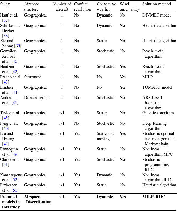


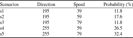


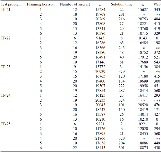


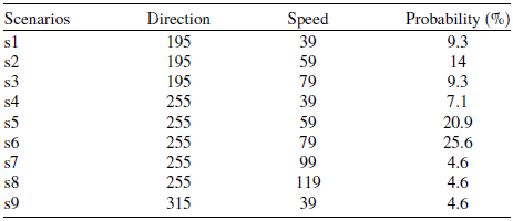



 Open access

