2 Basic dynamical equations

In 2-D isochoric Euler flows the field solutions are given in terms of a streamfunction $\unicode[STIX]{x1D713}(\boldsymbol{x},t)$ which provides the horizontal velocity $\boldsymbol{u}(\boldsymbol{x},t)$ and vorticity $\unicode[STIX]{x1D701}(\boldsymbol{x},t)$ fields,

(2.1a,b ) $$\begin{eqnarray}\boldsymbol{u}=-\unicode[STIX]{x1D735}\times (\unicode[STIX]{x1D713}\boldsymbol{k}),\quad \unicode[STIX]{x1D701}\equiv \boldsymbol{k}\boldsymbol{\cdot }\unicode[STIX]{x1D735}\times \boldsymbol{u}=\unicode[STIX]{x1D6FB}^{2}\unicode[STIX]{x1D713},\end{eqnarray}$$

where $\boldsymbol{k}$ is the vertical unit vector and $\unicode[STIX]{x1D735}$ is the 2-D gradient operator. The fundamental dynamical equation is the material conservation of vorticity

(2.2) $$\begin{eqnarray}\frac{\text{d}\unicode[STIX]{x1D701}}{\text{d}t}=\frac{\unicode[STIX]{x2202}\unicode[STIX]{x1D701}}{\unicode[STIX]{x2202}t}+\boldsymbol{u}\boldsymbol{\cdot }\unicode[STIX]{x1D735}\unicode[STIX]{x1D701}=\frac{\unicode[STIX]{x2202}}{\unicode[STIX]{x2202}t}\unicode[STIX]{x1D6FB}^{2}\unicode[STIX]{x1D713}+{\mathcal{J}}\{\unicode[STIX]{x1D713},\unicode[STIX]{x1D6FB}^{2}\unicode[STIX]{x1D713}\}=0,\end{eqnarray}$$

where ${\mathcal{J}}\{A(x,y),B(x,y)\}\equiv \unicode[STIX]{x2202}A/\unicode[STIX]{x2202}x\unicode[STIX]{x2202}B/\unicode[STIX]{x2202}y-\unicode[STIX]{x2202}B/\unicode[STIX]{x2202}x\unicode[STIX]{x2202}A/\unicode[STIX]{x2202}y$ is the Jacobian operator.

3 The two-dipole vortex as a conceptual embedded tripole model

Though it is possible to form an initial tripolar vortex structure, in polar coordinates $(r,\unicode[STIX]{x1D703})$ , with boundary radius $r=j_{1,1}$ , from a combination of circular Bessel modes 0 and 2 in the form $\unicode[STIX]{x1D701}(r,\unicode[STIX]{x1D703})=\unicode[STIX]{x1D701}_{0}[\text{J}_{0}(r)-\text{J}_{0}(j_{1,1})]+\unicode[STIX]{x1D701}_{2}\text{J}_{2}(k_{0}r)\cos (2\unicode[STIX]{x1D703})$ , this vorticity structure is unstable (see figure 3 and explanation in Viúdez (Reference Viúdez2019)). In the above, $\text{J}_{i}(r)$ is the Bessel function of the first kind and order  $i$ , $j_{i,m}$ is the $m$ -zero of $\text{J}_{i}(r)$ , $\{\unicode[STIX]{x1D701}_{0},\unicode[STIX]{x1D701}_{2}\}$ are the real constant modal amplitudes, and the constant $k_{0}\equiv j_{2,1}/j_{1,1}$ so that at the vortex boundary $\text{J}_{2}(k_{2}j_{1,1})=\text{J}_{2}(j_{2,1})=0$ . This instability occurs because, in a vortex, azimuthal mode-2 (as it happens to any azimuthal mode $i\geqslant 2$ , which may be thought of as consisting of $i$ dipoles) is a dispersive mode in the sense that the two dipoles, located inside a circle, tend to move apart, breaking the vortex, and disperse when mode-2 dominates ( $|\unicode[STIX]{x1D701}_{2}|\gg |\unicode[STIX]{x1D701}_{0}|$ ). When mode-0 dominates ( $|\unicode[STIX]{x1D701}_{0}|\gg |\unicode[STIX]{x1D701}_{2}|$ ), the mode-1 perturbation is circularly advected by the circular mode-0 and spiralizes so that its radial wavenumber increases indefinitely. In numerical simulations this perturbation is eventually dumped by numerical diffusion. When both amplitudes $|\unicode[STIX]{x1D701}_{0}|$ and $|\unicode[STIX]{x1D701}_{2}|$ are of the same order of magnitude, the unsteady vortex may evolve up to an orbital tripole vortex; although this occurs through a severe unsteady rearrangement of the vorticity field.

However, there is a way to assemble an embedded tripole from the superposition of two C–L dipoles. It is well known that an asymmetric circular C–L dipole (subscript  $D$ ) whose initial non-vanishing piecewise vorticity distribution is given by

(3.1) $$\begin{eqnarray}\hat{\unicode[STIX]{x1D701}}_{D}(r,\unicode[STIX]{x1D703};\unicode[STIX]{x1D703}_{0})\equiv \unicode[STIX]{x1D701}_{0}[\text{J}_{0}(r)-\text{J}_{0}(j_{1,1})]+\unicode[STIX]{x1D701}_{1}\text{J}_{1}(r)\cos (\unicode[STIX]{x1D703}+\unicode[STIX]{x1D703}_{0}),\quad r\leqslant j_{1,1},\end{eqnarray}$$

rotates rigidly with constant angular velocity $\unicode[STIX]{x1D6FA}_{0}=-\unicode[STIX]{x1D701}_{0}\text{J}_{0}(j_{1,1})/2$ , describing a circular trajectory with radius $R_{0}=|\unicode[STIX]{x1D701}_{1}/\unicode[STIX]{x1D701}_{0}|$ . Consider now a small dipolar amplitude $|\unicode[STIX]{x1D701}_{1}|<j_{1,1}|\unicode[STIX]{x1D701}_{0}|$ so that the trajectory curvature radius $R_{0}$ is shorter than the dipole extent radius  $j_{1,1}$ . In this case the dipole’s motion would resemble that of a vortex with one vorticity anomaly patch spinning with angular velocity $\unicode[STIX]{x1D6FA}_{0}$ around the inner core vortex. We superpose to this vorticity field the vorticity field of a twin dipole but with a phase shift $\unicode[STIX]{x0394}\unicode[STIX]{x1D703}_{0}=\unicode[STIX]{x03C0}$ and whose vortex centre is separated a distance $2R_{0}$ from its twin vortex dipole centre. Considered in isolation, these C–L dipoles rotate with the same angular velocity around the origin point. It is convenient now to work simultaneously with both polar $(r,\unicode[STIX]{x1D703})$ and Cartesian $(x,y)$ coordinates because the dipole internal structure is naturally defined in polar coordinates, while the dipole’s location is expressed more easily in Cartesian coordinates. Let the vorticity distribution in Cartesian $(x,y)$ coordinates of the C–L vortex dipole be

(3.2) $$\begin{eqnarray}\tilde{\unicode[STIX]{x1D701}}_{D}(x,y;\unicode[STIX]{x1D703}_{0})=\hat{\unicode[STIX]{x1D701}}_{D}(r(x,y),\unicode[STIX]{x1D703}(x,y);\unicode[STIX]{x1D703}_{0}),\end{eqnarray}$$

where the usual Cartesian to polar coordinates transformations are $r(x,y)=\sqrt{x^{2}+y^{2}}$ and $\unicode[STIX]{x1D703}(x,y)=\arctan y/x$ . For ease of reference denote the non-vanishing vorticity fields, in Cartesian coordinates, of the right (subscript  $R$ ) and left (subscript  $L$ ) twin dipoles as

(3.3) $$\begin{eqnarray}\displaystyle & \displaystyle \tilde{\unicode[STIX]{x1D701}}_{DR}(x,y)\equiv \tilde{\unicode[STIX]{x1D701}}_{D}(x+R_{0},y;0),\quad r(x+R_{0},y)\leqslant j_{1,1}, & \displaystyle\end{eqnarray}$$

(3.4) $$\begin{eqnarray}\displaystyle & \displaystyle \tilde{\unicode[STIX]{x1D701}}_{DL}(x,y)\equiv \tilde{\unicode[STIX]{x1D701}}_{D}(x-R_{0},y;\unicode[STIX]{x03C0}),\quad r(x-R_{0},y)\leqslant j_{1,1}. & \displaystyle\end{eqnarray}$$

Thus, the non-vanishing initial piecewise vorticity field of the two-dipole tripole model (subscript  $T$ ) is

(3.5) $$\begin{eqnarray}\tilde{\unicode[STIX]{x1D701}}_{T}(x,y)\equiv \tilde{\unicode[STIX]{x1D701}}_{DR}(x,y)+\tilde{\unicode[STIX]{x1D701}}_{DL}(x,y).\end{eqnarray}$$

Since, in isolation, the twin dipoles rotate with the same angular velocity $\unicode[STIX]{x1D6FA}_{0}=-\unicode[STIX]{x1D701}_{0}\text{J}_{0}(j_{1,1})/2$ describing a circle of radius $R_{0}$ it is expected that at a first, linear approximation, the vortex tripole structure (3.5) would rotate steadily with twice the angular velocity $\unicode[STIX]{x1D6FA}_{T}=-(2\unicode[STIX]{x1D701}_{0})\text{J}_{0}(j_{1,1})/2$ , because the two C–L amplitudes are added, around the geometrical centre of the two dipoles (the origin point $(x,y)=(0,0)$ ).

We calculate next the different terms in the vorticity conservation balance (2.2). To do so it is convenient, in order to avoid the irrelevant advection of the rigid vorticity field, to work in the reference frame rotating with angular velocity $\unicode[STIX]{x1D6FA}_{0}$ in which the C–L dipoles are steady. In this co-rotating reference frame the dipole vorticity $\widehat{\unicode[STIX]{x1D701}}_{D}$ is $\hat{\unicode[STIX]{x1D701}}_{D}$ given by (3.1) minus the vorticity of the rotating frame ( $2\unicode[STIX]{x1D6FA}_{0}=-\unicode[STIX]{x1D701}_{0}\text{J}_{0}(j_{1,1})$ ), that is

(3.6) $$\begin{eqnarray}\widehat{\unicode[STIX]{x1D701}}_{D}(r,\unicode[STIX]{x1D703};\unicode[STIX]{x1D703}_{0})\equiv \left\{\begin{array}{@{}ll@{}}\unicode[STIX]{x1D701}_{0}\text{J}_{0}(r)+\unicode[STIX]{x1D701}_{1}\text{J}_{1}(r)\cos (\unicode[STIX]{x1D703}+\unicode[STIX]{x1D703}_{0}), & r\leqslant j_{1,1}\\ \unicode[STIX]{x1D701}_{0}\text{J}_{0}(j_{1,1}), & j_{1,1}\leqslant r.\end{array}\right.\end{eqnarray}$$

We further define, in analogy to the previous definitions, in the co-rotating reference frame and in Cartesian coordinates the circular dipole

(3.7) $$\begin{eqnarray}\widetilde{\unicode[STIX]{x1D701}}_{D}(x,y;\unicode[STIX]{x1D703}_{0})=\widehat{\unicode[STIX]{x1D701}}_{D}(r(x,y),\unicode[STIX]{x1D703}(x,y);\unicode[STIX]{x1D703}_{0}),\end{eqnarray}$$

and the right $\widetilde{\unicode[STIX]{x1D701}}_{DR}(x,y)$ and left $\widetilde{\unicode[STIX]{x1D701}}_{DL}(x,y)$ dipoles are defined as (3.3) and (3.4), respectively. Finally, the two-dipole tripole vorticity model is given by

(3.8) $$\begin{eqnarray}\widetilde{\unicode[STIX]{x1D701}}_{T}(x,y)\equiv \widetilde{\unicode[STIX]{x1D701}}_{DR}(x,y)+\widetilde{\unicode[STIX]{x1D701}}_{DL}(x,y),\end{eqnarray}$$

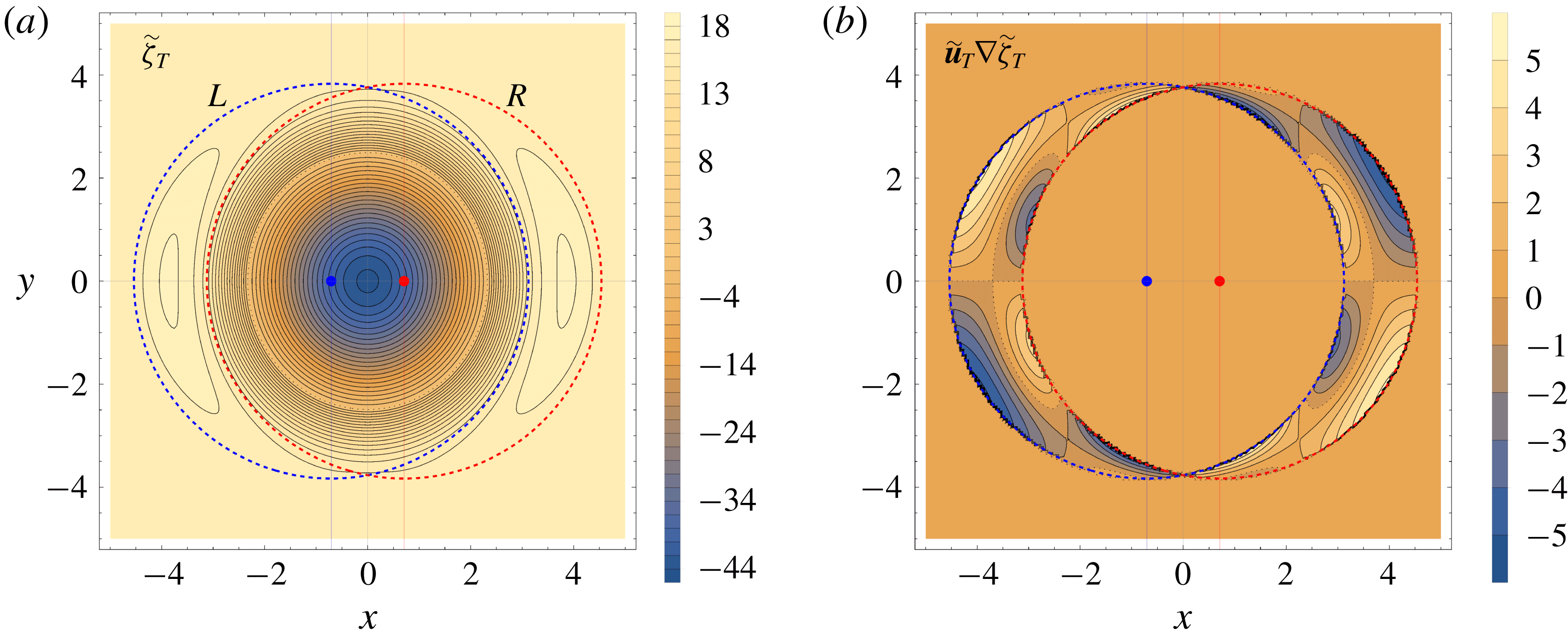
and is displayed in figure 1(a). The superposition of the two piecewise vorticity C–L dipole distributions defines four regions in the tripole domain: one inner region, defined as the intersection of the two interior vorticity dipole domains; two lateral regions ( $L$  and  $R$ ), occupied by only one interior dipole ( $L$  or  $R$ ) domain; and one outer region, defined as the intersection of the two exterior vorticity dipole domains.

Figure 1.

(a) The piecewise vorticity $\widetilde{\unicode[STIX]{x1D701}}_{T}(x,y)$ ( $\times 20$ ) of the two-dipole tripole model with modal amplitudes $\unicode[STIX]{x1D701}_{0}=-1$ and $\unicode[STIX]{x1D701}_{1}=-1/\sqrt{2}$ . The blue and red solid circles define, respectively, the boundaries of the left ( $L$ ) and right ( $R$ ) C–L dipoles. Contour intervals $\unicode[STIX]{x1D6E5}_{\unicode[STIX]{x1D701}}=1$ for $\widetilde{\unicode[STIX]{x1D701}}_{T}<0$ and $\unicode[STIX]{x1D6E5}_{\unicode[STIX]{x1D701}}=2$ for $\widetilde{\unicode[STIX]{x1D701}}_{T}>0$ . (b) Advection of the two-dipole tripole model $\widetilde{\boldsymbol{u}}_{T}\boldsymbol{\cdot }\unicode[STIX]{x1D735}\widetilde{\unicode[STIX]{x1D701}}_{T}$ ( $\times 2\times 10^{3}$ ). Contour interval $\unicode[STIX]{x1D6E5}=1$ .

In order to find up to what extent the two-dipole tripole (3.8) is a steadily rotating solution to the nonlinear equation of material conservation of vorticity (2.2) we calculate next the different advection terms involved. Since the product of the Bessel functions with the azimuthal modes, $\unicode[STIX]{x1D713}_{n}(r,\unicode[STIX]{x1D703})\equiv \text{J}_{n}(r)\exp (\text{i}n\unicode[STIX]{x1D703})$ , are the eigenfunctions of the Laplacian in polar coordinates, $\unicode[STIX]{x1D6FB}^{2}\unicode[STIX]{x1D713}_{n}=-\unicode[STIX]{x1D713}_{n}$ , the advection of vorticity of every mode, given by the Jacobian ${\mathcal{J}}\{\unicode[STIX]{x1D713}_{n},\unicode[STIX]{x1D6FB}^{2}\unicode[STIX]{x1D713}_{n}\}$ in (2.2), vanishes. The nonlinear advection involving two modes  $i$ , $j$ also cancels out since ${\mathcal{J}}\{\unicode[STIX]{x1D713}_{i},\unicode[STIX]{x1D6FB}^{2}\unicode[STIX]{x1D713}_{j}\}=-{\mathcal{J}}\{\unicode[STIX]{x1D713}_{j},\unicode[STIX]{x1D6FB}^{2}\unicode[STIX]{x1D713}_{i}\}$ . Thus, the advection of vorticity in the isolated dipole vanishes and the C–L dipole remains steady. The advection of vorticity vanishes as well in the interior tripole when the two dipoles are simultaneously present, because the advection involving any pair of modes  $i$ , $j\in \{0,1\}$ includes the vortex crossing terms

(3.9) $$\begin{eqnarray}\widetilde{\boldsymbol{u}}_{Li}\boldsymbol{\cdot }\unicode[STIX]{x1D735}\widetilde{\unicode[STIX]{x1D701}}_{Rj}+\widetilde{\boldsymbol{u}}_{Rj}\boldsymbol{\cdot }\unicode[STIX]{x1D735}\widetilde{\unicode[STIX]{x1D701}}_{Li}={\mathcal{J}}\{\widetilde{\unicode[STIX]{x1D719}}_{Li},-\widetilde{\unicode[STIX]{x1D719}}_{Rj}\}+{\mathcal{J}}\{\widetilde{\unicode[STIX]{x1D719}}_{Rj},-\widetilde{\unicode[STIX]{x1D719}}_{Li}\}=0.\end{eqnarray}$$

We note that other vortex models, such as the Lamb–Oseen or Batchelor vortices, do not satisfy this superposition property. The vorticity advection in the exterior tripole vanishes as well, since the exterior vorticity is constant. Therefore, there remains only the vorticity advection in the lateral regions, or lateral vortices, which in the left lateral vortex is due to the advection of the $L$ vortex vorticity by the $R$ vortex velocity $\widetilde{\boldsymbol{u}}_{R}\boldsymbol{\cdot }\unicode[STIX]{x1D735}\widetilde{\unicode[STIX]{x1D701}}_{L}$ , and in the right lateral vortex is due to the advection of the $R$ vortex vorticity by the $L$ vortex velocity $\widetilde{\boldsymbol{u}}_{L}\boldsymbol{\cdot }\unicode[STIX]{x1D735}\widetilde{\unicode[STIX]{x1D701}}_{R}$ . For example, we may check (appendix A) that the vorticity advection in the left lateral region is

(3.10) $$\begin{eqnarray}\displaystyle \widetilde{\boldsymbol{u}}_{R}\boldsymbol{\cdot }\unicode[STIX]{x1D735}\widetilde{\unicode[STIX]{x1D701}}_{L}(x,y) & = & \displaystyle \frac{y\unicode[STIX]{x1D719}_{1}^{2}\text{J}_{0}(j_{1,1})}{2(x_{-}^{2}+y^{2})^{2}}\left[\vphantom{{\displaystyle \frac{2j_{1,1}^{2}}{\sqrt{x_{+}^{2}+y^{2}}}}}(x_{+})\frac{(x_{-}^{2}+y^{2})^{2}-j_{1,1}^{2}(x_{-}^{2}+y^{2}-4R_{0}x_{-})}{x_{+}^{2}+y^{2}}\text{J}_{2}\left(\sqrt{x_{+}^{2}+y^{2}}\right)\right.\nonumber\\ \displaystyle & & \displaystyle +\left.(x_{-})\frac{2j_{1,1}^{2}}{\sqrt{x_{+}^{2}+y^{2}}}\text{J}_{1}\left(\sqrt{x_{+}^{2}+y^{2}}\right)\right],\end{eqnarray}$$

where $x_{\pm }\equiv x\pm \unicode[STIX]{x1D719}_{1}/\unicode[STIX]{x1D719}_{0}$ . The complete vorticity advection distribution is shown in figure 1(b). The vorticity advection (3.10) vanishes for $\unicode[STIX]{x1D719}_{1}=0$ (this case lacks the dipolar mode, $R_{0}=0$ ), vanishes also along the axis $y=0$ , and depends linearly on $\unicode[STIX]{x1D719}_{1}^{2}$ , which is assumed small compared to $\unicode[STIX]{x1D719}_{0}^{2}$ . Note that (3.10) depends on $\unicode[STIX]{x1D719}_{0}$ through $x\pm \unicode[STIX]{x1D719}_{1}/\unicode[STIX]{x1D719}_{0}$ and $R_{0}\equiv \unicode[STIX]{x1D719}_{1}/\unicode[STIX]{x1D719}_{0}$ . We recall that when the two vorticity fields are added in (3.8) the constant background vorticity field is doubled to $2\unicode[STIX]{x1D701}_{0}\text{J}_{0}(j_{1,1})$ , and therefore the two-dipole tripole model is expected to rotate with an angular velocity $\unicode[STIX]{x1D6FA}_{T}=-\unicode[STIX]{x1D701}_{0}\text{J}_{0}(j_{1,1})$ .

Figure 2.

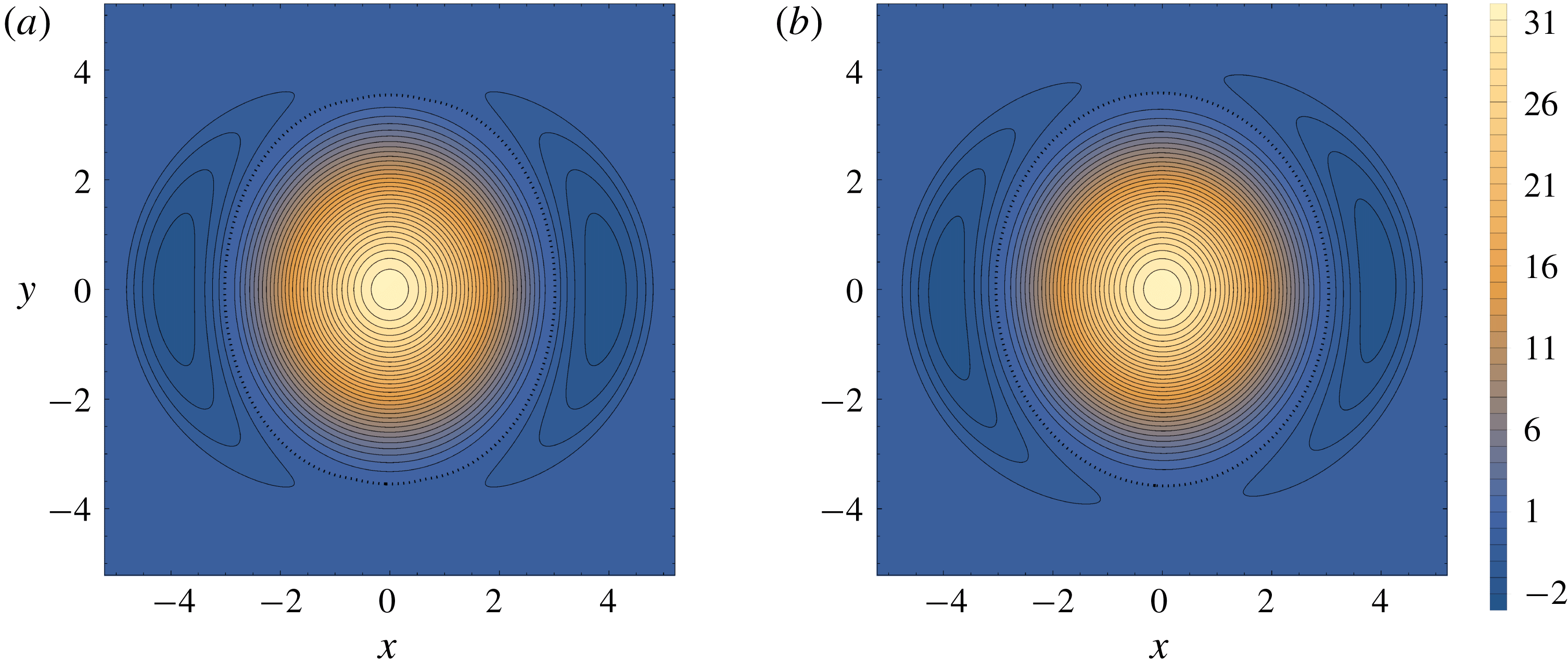
The vorticity distribution $\tilde{\unicode[STIX]{x1D701}}_{T}(x,y,t_{0})$ ( $\times 20$ ) from numerical simulations of the two-dipole tripole model, with amplitudes $\unicode[STIX]{x1D701}_{0}=\unicode[STIX]{x1D701}_{1}=1/2$ , at (a)  $t_{0}=0$ , and (b)  $t_{0}=500$ . Contour intervals $\unicode[STIX]{x1D6E5}_{\unicode[STIX]{x1D701}}=0.5$ ( $\tilde{\unicode[STIX]{x1D701}}_{T}<0$ ) and $\unicode[STIX]{x1D6E5}_{\unicode[STIX]{x1D701}}=1$ ( $\tilde{\unicode[STIX]{x1D701}}_{T}>0$ ). The black thick dotted line is the contour $\tilde{\unicode[STIX]{x1D701}}_{T}=0$ . The background numerical vorticity is $\bar{\unicode[STIX]{x1D701}}_{N}\simeq -0.02064$ .

Numerical simulations were carried out using a 2-D pseudo-spectral code where the vorticity field $\unicode[STIX]{x1D701}(x,y,t)$ is numerically integrated in a double-periodic domain using an explicit leap-frog time-stepping method, together with a weak Robert–Asselin time filter to avoid the decoupling of even and odd time levels (as in Dritschel & Viúdez Reference Dritschel and Viúdez2003). Spatial fields are computed using the pseudo-spectral method, wherein spatial derivatives are computed in spectral space, while the advective nonlinear products are computed on the physical grid, and fast Fourier transforms are used to go from one representation to the other. Numerical simulations with a moderate resolution ( $1024^{2}$ grid points), initialized with the two-dipole tripole vorticity distribution (figure 2 a) confirmed that the tripole was stable and soon reaches a rigidly rotating vorticity field (figure 2 b and supplementary movie 1, available at https://doi.org/10.1017/jfm.2019.730). In a time period $\unicode[STIX]{x1D6E5}_{T}=500$ the tripole undergoes $N_{R}=29/2$ anticlockwise rotations. Since the numerical pseudo-spectral algorithm requires zero spatial average vorticity there is a small background constant vorticity in figure 2 equal to $\bar{\unicode[STIX]{x1D701}}_{N}\simeq -0.02064$ , which provides a small correction to the tripole angular velocity $\unicode[STIX]{x1D6FA}_{T}=2\unicode[STIX]{x03C0}N_{R}/\unicode[STIX]{x1D6E5}_{T}-\bar{\unicode[STIX]{x1D701}}_{N}/2\simeq 0.1822+0.0103\simeq 0.192$ . This angular velocity compares well with the angular velocity of an isolated C–L dipole, with double mode-0 amplitude, $\unicode[STIX]{x1D6FA}_{T}=-\unicode[STIX]{x1D701}_{0}\text{J}_{0}(j_{1,1})\simeq 0.201$ .

It is also possible to construct asymmetric tripoles selecting different modal amplitudes $\unicode[STIX]{x1D719}_{L0}\neq \unicode[STIX]{x1D719}_{R0}$ for the left ( $L$ ) and $\unicode[STIX]{x1D719}_{L1}\neq \unicode[STIX]{x1D719}_{R1}$ for the right ( $R$ ) C–L dipoles. For example, setting without loss of generality $\unicode[STIX]{x1D719}_{L0}=1$ , and positive modal amplitudes such that the left $R_{L}\equiv \unicode[STIX]{x1D719}_{L0}/\unicode[STIX]{x1D719}_{L1}$ and right $R_{R}\equiv \unicode[STIX]{x1D719}_{R0}/\unicode[STIX]{x1D719}_{R1}$ C–L dipole trajectory radius coincide ( $R_{L}=R_{R}$ ), with $\unicode[STIX]{x1D719}_{L1}\neq \unicode[STIX]{x1D719}_{R1}$ , leads to steadily rotating asymmetric tripoles whose centre (the point where vorticity reaches an extremum) remains approximately at the origin point. Positive modal amplitudes such that the left and right C–L dipole trajectory radius differ ( $R_{L}\neq R_{R}$ ) lead to asymmetric tripoles whose centre approximately describes circles around the origin point. Asymmetric fixed-centre tripoles ( $R_{L}=R_{R}$ ) were found to be numerically more stable than the asymmetric rotating-centre tripoles ( $R_{L}\neq R_{R}$ ).

Considering the simplicity of the symmetric two-dipole tripole distribution, it is surprising that the numerical simulations show very similar initial and steadily rotating vorticity distributions (figure 2). This implies that the two-dipole tripole model is a reasonably good conceptual model of an embedded tripole. A closer look at largely augmented images of the time-evolving interior vorticity isolines reveals that their shapes change until reaching, in the steadily rotating state (figure 2 b), a confocal elliptical geometry. This fact suggests the search for steady and stable elliptical vortex tripoles carried out in the next section.

4 Steadily rotating tripole model with distributed vorticity

This section provides exact solutions, with continuous vorticity, of stable and steadily rotating embedded tripole vortices. Guided by the results obtained in the previous section using the two-dipole tripole model we look for steady streamfunction solutions $\unicode[STIX]{x1D719}(\unicode[STIX]{x1D707},\unicode[STIX]{x1D708})=R(\unicode[STIX]{x1D707})\unicode[STIX]{x1D6F7}(\unicode[STIX]{x1D708})$ separable in elliptic coordinates $(\unicode[STIX]{x1D707},\unicode[STIX]{x1D708})$ with $0\leqslant \unicode[STIX]{x1D707}<\infty$ and $-\unicode[STIX]{x03C0}\leqslant \unicode[STIX]{x1D708}<\unicode[STIX]{x03C0}$ . Elliptic coordinates $(\unicode[STIX]{x1D707},\unicode[STIX]{x1D708})$ are defined through the usual relation to Cartesian coordinates $(x,y)$ :

(4.1a,b ) $$\begin{eqnarray}x(\unicode[STIX]{x1D707},\unicode[STIX]{x1D708};f)=f\cosh \unicode[STIX]{x1D707}\cos \unicode[STIX]{x1D708},\quad y(\unicode[STIX]{x1D707},\unicode[STIX]{x1D708};f)=f\sinh \unicode[STIX]{x1D707}\sin \unicode[STIX]{x1D708},\end{eqnarray}$$

where the two foci are located at $(x,y)=(\pm f,0)$ . Thus, the streamfunction $\unicode[STIX]{x1D719}(\unicode[STIX]{x1D707},\unicode[STIX]{x1D708})$ must satisfy (2.2) in the steady state, which becomes the Helmholtz equation in elliptic coordinates,

(4.2) $$\begin{eqnarray}\unicode[STIX]{x1D6FB}^{2}\unicode[STIX]{x1D719}(\unicode[STIX]{x1D707},\unicode[STIX]{x1D708})=\frac{\unicode[STIX]{x1D719}_{\unicode[STIX]{x1D707}\unicode[STIX]{x1D707}}(\unicode[STIX]{x1D707},\unicode[STIX]{x1D708})+\unicode[STIX]{x1D719}_{\unicode[STIX]{x1D708}\unicode[STIX]{x1D708}}(\unicode[STIX]{x1D707},\unicode[STIX]{x1D708})}{f^{2}(\sinh ^{2}\unicode[STIX]{x1D707}+\sin ^{2}\unicode[STIX]{x1D708})}=-k^{2}\unicode[STIX]{x1D719}(\unicode[STIX]{x1D707},\unicode[STIX]{x1D708}),\end{eqnarray}$$

where $k$ is the wavenumber. The solutions of (4.2) are the ordinary (angular) and the modified (radial) Mathieu equations (see, for example, McLachlan Reference McLachlan1951; Abramowitz & Stegun Reference Abramowitz and Stegun1964; Gutiérrez-Vega et al. Reference Gutiérrez-Vega, Rodríguez-Dagnino, Meneses-Nava and Chávez-Cerda2003)

(4.3) $$\begin{eqnarray}\displaystyle & \displaystyle \unicode[STIX]{x1D6F7}^{\prime \prime }(\unicode[STIX]{x1D708})+(a-2q\cos 2\unicode[STIX]{x1D708})\unicode[STIX]{x1D6F7}(\unicode[STIX]{x1D708})=0, & \displaystyle\end{eqnarray}$$

(4.4) $$\begin{eqnarray}\displaystyle & \displaystyle R^{\prime \prime }(\unicode[STIX]{x1D707})-(a-2q\cosh 2\unicode[STIX]{x1D707})R(\unicode[STIX]{x1D707})=0, & \displaystyle\end{eqnarray}$$

where $a$ is the separation constant and $q\equiv f^{2}k^{2}/4$ . The angular Mathieu equation (4.3) has two families of independent solutions: namely the even, cosine-elliptic angular Mathieu functions $\unicode[STIX]{x1D6F7}_{m}(\unicode[STIX]{x1D708})=\text{ce}_{m}(\unicode[STIX]{x1D708};q)$ , $m=0,1,2,\ldots ,$ and the odd, sine-elliptic angular Mathieu functions $\unicode[STIX]{x1D6F7}_{m}(\unicode[STIX]{x1D708})=\text{se}_{m}(\unicode[STIX]{x1D708};q)$ , $m=1,2,\ldots ,$ where $m$ is the order. The value of the separation constant $a=a_{r}(r;q)$ that satisfies the angular periodicity conditions is the characteristic value for the even Mathieu function with characteristic exponent $r$ and parameter  $q$ . When $q>0$ the solutions $R_{m}(\unicode[STIX]{x1D707})$ to (4.4) are the even (e) and odd (o) oscillatory radial Mathieu functions of the first kind ( $\text{Je}(\unicode[STIX]{x1D707};q)$ and $\text{Jo}(\unicode[STIX]{x1D707};q)$ ) and second kind ( $\text{Ne}(\unicode[STIX]{x1D707};q)$ and $\text{No}(\unicode[STIX]{x1D707};q)$ ).

Figure 3.

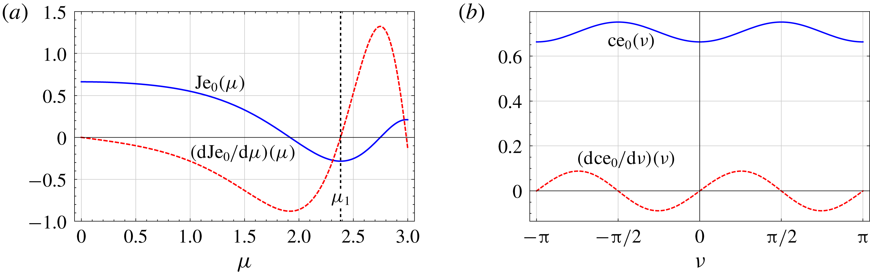
The even order-0 Mathieu functions and their derivatives. (a) Radial functions $\text{Je}_{0}(\unicode[STIX]{x1D707})$ and $\text{Je}_{0}^{\prime }(\unicode[STIX]{x1D707})$ . The first zero $\unicode[STIX]{x1D707}_{1}\simeq 2.3833$ of $\text{Je}_{0}^{\prime }(\unicode[STIX]{x1D707})$ is indicated. (b) Angular functions $\text{ce}_{0}(\unicode[STIX]{x1D708})$ and $\text{ce}_{0}^{\prime }(\unicode[STIX]{x1D708})$ . Function $\text{ce}_{0}(\unicode[STIX]{x1D708})$ is similar to a shifted $-\cos 2\unicode[STIX]{x1D708}$ function. Parameter $q=1/8$ corresponding to $f=1/\sqrt{2}$ and $k=1$ .

Figure 4.

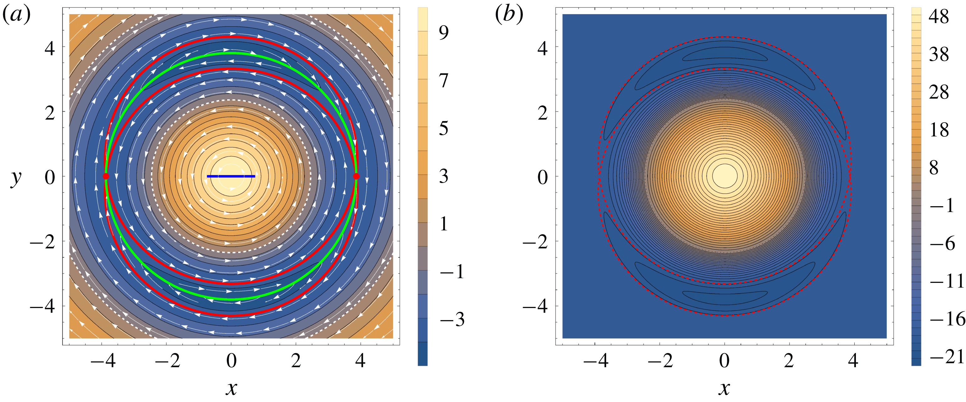
(a) Mathieu distribution $\text{Je}_{0}(\unicode[STIX]{x1D707}(x,y);q)\text{ce}_{0}(\unicode[STIX]{x1D708}(x,y);q)$ ( $\times 20$ , thin black contours) for wavenumber $k=1$ and foci $f=1/\sqrt{2}$ . The blue horizontal line joins the foci points $(\pm f,0)$ . The white lines with arrows are the streamlines of (4.6). The two red dots are the critical points $(\unicode[STIX]{x1D707},\unicode[STIX]{x1D708})=(\unicode[STIX]{x1D707}_{1},0)$ and $(\unicode[STIX]{x1D707},\unicode[STIX]{x1D708})=(\unicode[STIX]{x1D707}_{1},\unicode[STIX]{x03C0})$ . The green curve is the ellipse $\unicode[STIX]{x1D707}(\unicode[STIX]{x1D708})=\unicode[STIX]{x1D707}_{1}$ passing through the critical points. The red curves are the isolines of $\text{Je}_{0}(\unicode[STIX]{x1D707})\text{ce}_{0}(\unicode[STIX]{x1D708})=\text{Je}_{0}(\unicode[STIX]{x1D707}_{1})\text{ce}_{0}(0)$ . (b) The piecewise vorticity field $\unicode[STIX]{x1D701}(x,y)=\text{Je}_{0}(\unicode[STIX]{x1D707})\text{ce}_{0}(\unicode[STIX]{x1D708})$ ( $\unicode[STIX]{x1D707}\leqslant \unicode[STIX]{x1D707}_{B}(\unicode[STIX]{x1D708})$ ) $\unicode[STIX]{x1D701}(x,y)=\text{Je}_{0}(\unicode[STIX]{x1D707}_{1})\text{ce}_{0}(0)$ ( $\unicode[STIX]{x1D707}>\unicode[STIX]{x1D707}_{B}(\unicode[STIX]{x1D708})$ ), ( $\times 20$ , thin black contours). Contour intervals are $\unicode[STIX]{x1D6E5}_{\unicode[STIX]{x1D701}}=1$ ( $\unicode[STIX]{x1D701}<0$ ) and $\unicode[STIX]{x1D6E5}_{\unicode[STIX]{x1D701}}=2$ ( $\unicode[STIX]{x1D701}>0$ ). The white thin dotted contour is the zero-vorticity isoline. The red dashed curves are the isolines of $\unicode[STIX]{x1D701}=\text{Je}_{0}(\unicode[STIX]{x1D707}_{1})\text{ce}_{0}(0)$ .

The interior vorticity $\unicode[STIX]{x1D701}_{i}(\unicode[STIX]{x1D707},\unicode[STIX]{x1D708})$ of the tripole vortex model introduced here is given by the simplest mode, namely the even order-0 Mathieu functions of the first kind

(4.5) $$\begin{eqnarray}\unicode[STIX]{x1D701}_{i}(\unicode[STIX]{x1D707},\unicode[STIX]{x1D708};q)=-\unicode[STIX]{x1D719}_{i}(\unicode[STIX]{x1D707},\unicode[STIX]{x1D708};q)=\unicode[STIX]{x1D701}_{0}\text{Je}_{0}(\unicode[STIX]{x1D707};q)\text{ce}_{0}(\unicode[STIX]{x1D708};q).\end{eqnarray}$$

The order-0 radial and angular Mathieu functions $\text{Je}_{0}(\unicode[STIX]{x1D707})$ and $\text{ce}_{0}(\unicode[STIX]{x1D708})$ are shown in figure 3, and the corresponding field solution $\text{Je}_{0}(\unicode[STIX]{x1D707};q)\text{ce}_{0}(\unicode[STIX]{x1D708};q)$ in figure 4(a). The interior velocity is

(4.6) $$\begin{eqnarray}\boldsymbol{u}_{i}(\unicode[STIX]{x1D707},\unicode[STIX]{x1D708})=-\unicode[STIX]{x1D735}\times (\unicode[STIX]{x1D719}_{i}(\unicode[STIX]{x1D707},\unicode[STIX]{x1D708})\boldsymbol{k})=\frac{-\text{Je}_{0}(\unicode[STIX]{x1D707})\text{ce}_{0}^{\prime }(\unicode[STIX]{x1D708})\boldsymbol{e}_{\unicode[STIX]{x1D707}}+\text{Je}_{0}^{\prime }(\unicode[STIX]{x1D707})\text{ce}_{0}(\unicode[STIX]{x1D708})\boldsymbol{e}_{\unicode[STIX]{x1D708}}}{f\sqrt{\sinh ^{2}\unicode[STIX]{x1D707}+\sin ^{2}\unicode[STIX]{x1D708}}}.\end{eqnarray}$$

The boundary separating the interior vortical flow from the exterior potential flow, say curve $\unicode[STIX]{x1D707}=\unicode[STIX]{x1D707}_{B}(\unicode[STIX]{x1D708})$ , is set as the external branch (external red curve in figure 4 a) of the vorticity isoline passing through the first critical points $(\unicode[STIX]{x1D707}_{1},0)$ and $(\unicode[STIX]{x1D707}_{1},\unicode[STIX]{x03C0})$ , where $\unicode[STIX]{x1D707}_{1}$ is the first minimum of $\text{Je}_{0}(\unicode[STIX]{x1D707})$ , or first zero (excluding $\unicode[STIX]{x1D707}=0$ ) of $\text{Je}_{0}^{\prime }(\unicode[STIX]{x1D707})$ (figure 3 a). Thus, the separatrix vorticity value is

(4.7) $$\begin{eqnarray}\unicode[STIX]{x1D701}(\unicode[STIX]{x1D707}_{B}(\unicode[STIX]{x1D708}),\unicode[STIX]{x1D708})=\unicode[STIX]{x1D701}(\unicode[STIX]{x1D707}_{1},0)=\unicode[STIX]{x1D701}_{l}\simeq 0.1879.\end{eqnarray}$$

The other relevant curve passing through the critical points is a vorticity extremum and is the ellipse $\unicode[STIX]{x1D707}(\unicode[STIX]{x1D708})=\unicode[STIX]{x1D707}_{1}$ (green curve in figure 4 a). Along this curve $\text{Je}_{0}^{\prime }(\unicode[STIX]{x1D707}_{1})=0$ and the velocity has only a $\unicode[STIX]{x1D707}$ -component,

(4.8) $$\begin{eqnarray}\boldsymbol{u}(\unicode[STIX]{x1D707}_{1},\unicode[STIX]{x1D708})=-\frac{\text{Je}_{0}(\unicode[STIX]{x1D707}_{1})\text{ce}_{0}^{\prime }(\unicode[STIX]{x1D708})}{f\sqrt{\sinh ^{2}\unicode[STIX]{x1D707}_{1}+\sin ^{2}\unicode[STIX]{x1D708}}}\,\boldsymbol{e}_{\!\unicode[STIX]{x1D707}}.\end{eqnarray}$$

Finally, the non-vanishing vorticity of the embedded tripole is given, in the fixed reference frame at the initial time $t_{0}=0$ , by

(4.9) $$\begin{eqnarray}\unicode[STIX]{x1D701}(\unicode[STIX]{x1D707},\unicode[STIX]{x1D708},t_{0})=\unicode[STIX]{x1D701}_{0}(\text{Je}_{0}(\unicode[STIX]{x1D707})\text{ce}_{0}(\unicode[STIX]{x1D708})-\text{Je}_{0}(\unicode[STIX]{x1D707}_{1})\text{ce}_{0}(0)),\quad \unicode[STIX]{x1D707}\leqslant \unicode[STIX]{x1D707}_{B}(\unicode[STIX]{x1D708}).\end{eqnarray}$$

In the case of approaching circular geometry ( $f\rightarrow 0$ ) the radial Mathieu functions $\text{Je}_{n}(\unicode[STIX]{x1D707})$ converge to the Bessel functions $\text{J}_{n}(r)$ , curves $\unicode[STIX]{x1D707}=\unicode[STIX]{x1D707}_{B}(\unicode[STIX]{x1D708})$ and $\unicode[STIX]{x1D707}=\unicode[STIX]{x1D707}_{1}$ collapse to the circle of radius $r=j_{1,1}\simeq 3.8317$ , and the tripole converges to the circular mode of the C–L dipole. Since $\text{J}_{0}^{\prime }(r)=-\text{J}_{1}(r)$ , the C–L dipole has, at its boundary radius $r=j_{1,1}$ , both vanishing radial velocity, given by $\text{J}_{0}^{\prime }(j_{1,1})=-\text{J}_{1}(j_{1,1})=0$ , and constant vorticity, given by $\text{J}_{0}(j_{1,1})$ . This is not, however, the case in the embedded vortex tripole.

The complicated boundary conditions at $\unicode[STIX]{x1D707}=\unicode[STIX]{x1D707}_{B}(\unicode[STIX]{x1D708})$ make it difficult to find a closed-form solution of the exterior streamfunction, which is not provided here. The exterior streamfunction, however, can always be obtained numerically from the inversion of $\unicode[STIX]{x1D701}=-\unicode[STIX]{x1D6FB}^{2}\unicode[STIX]{x1D719}$ , which is straightforward using the 2-D Fourier transform in a rectangular domain. Numerical simulations using a pseudo-spectral code with $2048^{2}$ grid points confirmed the stability of the embedded tripole (supplementary movie 2) after some time adjustment in the lateral vortices related to the instability at the critical points. 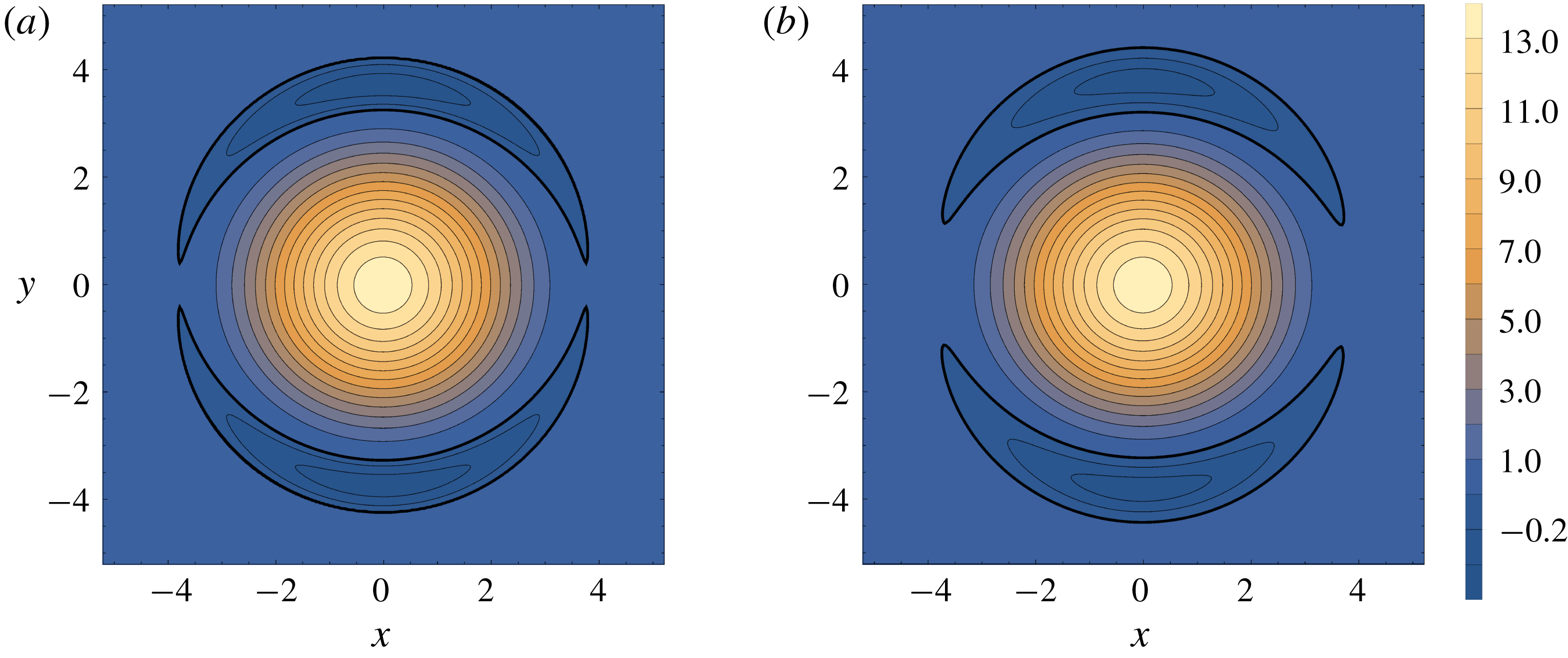In a time interval $\unicode[STIX]{x1D6E5}_{T}=4240$ (figure 5) the tripole performed $N_{R}=60$ rotations, which, taking into account a small background constant numerical vorticity $\bar{\unicode[STIX]{x1D701}}_{N}\simeq -0.00331$ , results in an angular velocity $\unicode[STIX]{x1D6FA}_{0}=2\unicode[STIX]{x03C0}N_{R}/\unicode[STIX]{x1D6E5}_{T}-\bar{\unicode[STIX]{x1D701}}_{N}/2\simeq 0.0889+0.00166\simeq 0.091$ . This value compares well with the theoretical angular velocity $\unicode[STIX]{x1D701}_{l}/2=\text{Je}_{0}(\unicode[STIX]{x1D707}_{1})\text{ce}_{0}(0)/2\simeq 0.094$ .

5 Concluding remarks

We have found exact solutions of steady and stable 2-D tripoles with distributed vorticity and small-amplitude embedded lateral vortices. The solutions are given in elliptical coordinates $(\unicode[STIX]{x1D707},\unicode[STIX]{x1D708})$ by the even radial and angular Mathieu function of order zero $\text{Je}_{0}(\unicode[STIX]{x1D707})\text{ce}_{0}(\unicode[STIX]{x1D708})$ truncated at the external branch of the first separation streamline. The tripole rotates with an angular velocity $\unicode[STIX]{x1D6FA}_{0}=-\unicode[STIX]{x1D701}_{0}\text{Je}_{0}(\unicode[STIX]{x1D707}_{1})\text{ce}_{0}(0)/2\simeq 0.09397\unicode[STIX]{x1D701}_{0}$ , where $\unicode[STIX]{x1D707}_{1}$ is the first zero of $\text{Je}_{0}^{\prime }(\unicode[STIX]{x1D707})$ . Although, due to the difficulties associated with the Mathieu functions, this tripole model is difficult to handle, it is possible to conceptually think of embedded 2-D tripoles as the superposition of two C–L dipoles separated a distance equal to twice the distance of their individual trajectory curvature radius. However, the amplitude of these lateral vortices is small, and these embedded tripoles may be otherwise regarded as single stable elliptical vortices. Nevertheless, the presence of the lateral vortices is important to preserve the vortex ellipticity against vortex axis-symmetrization.

It is straightforward to extend the two-dipole tripole model to the superposition of $n\geqslant 3$ dipoles ( $n$ equidistant lateral vortices with an azimuthal phase difference $\unicode[STIX]{x0394}\unicode[STIX]{x1D703}=2\unicode[STIX]{x03C0}/n$ ). However, numerical experiments showed that these embedded $n$ -dipoles were unstable and evolved into stable circular vortices.

Figure 5.

The piecewise vorticity $\unicode[STIX]{x1D701}(x,y,t_{0})$ ( $\times 20$ ) of the continuous tripole model with amplitude $\unicode[STIX]{x1D701}_{0}=1$ and foci $f=1/\sqrt{2}$ , at (a) the initial time $t_{0}=0$ , and (b) at $t_{0}=4240$ . Contour intervals are $\unicode[STIX]{x1D6E5}_{\unicode[STIX]{x1D701}}=0.2$ ( $\unicode[STIX]{x1D701}<0$ ) and $\unicode[STIX]{x1D6E5}_{\unicode[STIX]{x1D701}}=1$ ( $\unicode[STIX]{x1D701}>0$ ). The black thick solid contour is the zero-vorticity isoline.

These results may be relevant also to plasma physics, where tripolar vortices have been observed (Okamoto et al. Reference Okamoto, Hara, Nagaoka, Yoshimura, Vranješ, Kono and Tanaka2003), as well as to baroclinic three-dimensional flows in the ocean (Pingree & Le Cann Reference Pingree and Le Cann1992). In fact, a three-dimensional quasi-geostrophic two-dipole tripole model is possible using exact quasi-geostrophic dipole solutions. Investigation along this line of research is left for future work.