2. Problem formulation

Throughout this paper, we use an asterisk to represent dimensional quantities. For non-dimensional quantities, we use normal letters. Consider a spherical bubble attached to the tip of a tube, where the tube is submerged to a depth $h^*$ in a rigid container outside the tube. The container suddenly experiences an impulse at its bottom due to an impact, and the jet bursts from the bottom of the controlled spherical bubble. The angle between the meniscus of the bubble and the horizontal line is defined as $\theta$ . The radius of the cylindrical tube inside the container is $R^*$ , and that of the container is $r^*$ . Figure 1 shows a schematic of the geometric parameters.

We define the velocities before and after the impact as $\boldsymbol{u}^*(0)$ and $\boldsymbol{u}^*(\tau ^*)$ , where $\tau ^*$ is an impact duration period. According to a classical result from Batchelor (Reference Batchelor2000) and work on liquid jets by Antkowiak et al. (Reference Antkowiak, Bremond, Le Dizès and Villermaux2007), it is assumed that the fluid is inviscid and irrotational during the transient time of the impulse. The velocity of the liquid $\boldsymbol{u}^*$ is then governed by

(2.1) \begin{align} \frac {\partial \boldsymbol{u}^*}{\partial t^*} = -\frac {1}{\rho ^*}\boldsymbol{\nabla} ^* p^*, \end{align}

where $\boldsymbol{\nabla} ^*$ is a dimensional gradient operator, $p^*$ is a fluid pressure, and $\rho ^*$ is the density of the liquid. By integrating (2.1) with respect to the short time period of the impact $\tau ^*$ , the velocity $\boldsymbol{u}^*(\tau ^*)$ satisfies

(2.2) \begin{align} \boldsymbol{u}^*(\tau ^*) - \boldsymbol{u}^*(0)= -\frac {1}{\rho ^*} \boldsymbol{\nabla} ^* \varPi ^*. \end{align}

Here, $\varPi ^*$ is the pressure impulse defined by the integral of the pressure $p^*$ over the short impact duration $\tau ^*$ . Since the flow is assumed to be incompressible, the pressure impulse $\varPi ^*$ satisfies the 3-D Laplace equation in the region filled with liquid, i.e.

(2.3) \begin{align} {\nabla} ^{*2} \varPi ^* = 0 \end{align}

in the cylindrical domain outside the bubble. The jet velocity $\boldsymbol{u}^*(\tau ^*)$ is calculated using the spatial derivative of $\varPi ^*$ , as given in (2.2) after obtaining $\varPi ^*$ .

It is convenient to non-dimensionalise the pressure impulse and the coordinates, i.e. $\varPi ^* = \varPi \,\rho ^* U^*_0 R^*$ and $(x^*,y^*,z^*) = (R^*x,R^*y,R^* z)$ . With this scaling, the radius of the inner tube is always set to $1$ . Here, $U_0^*$ is the velocity of the container in the $z^*$ -direction at the initial time due to the elastic collision at the bottom. Furthermore, the non-dimensional geometric parameters are defined by $h:=h^*/R^*$ and $\lambda :=R^*/r^*$ . 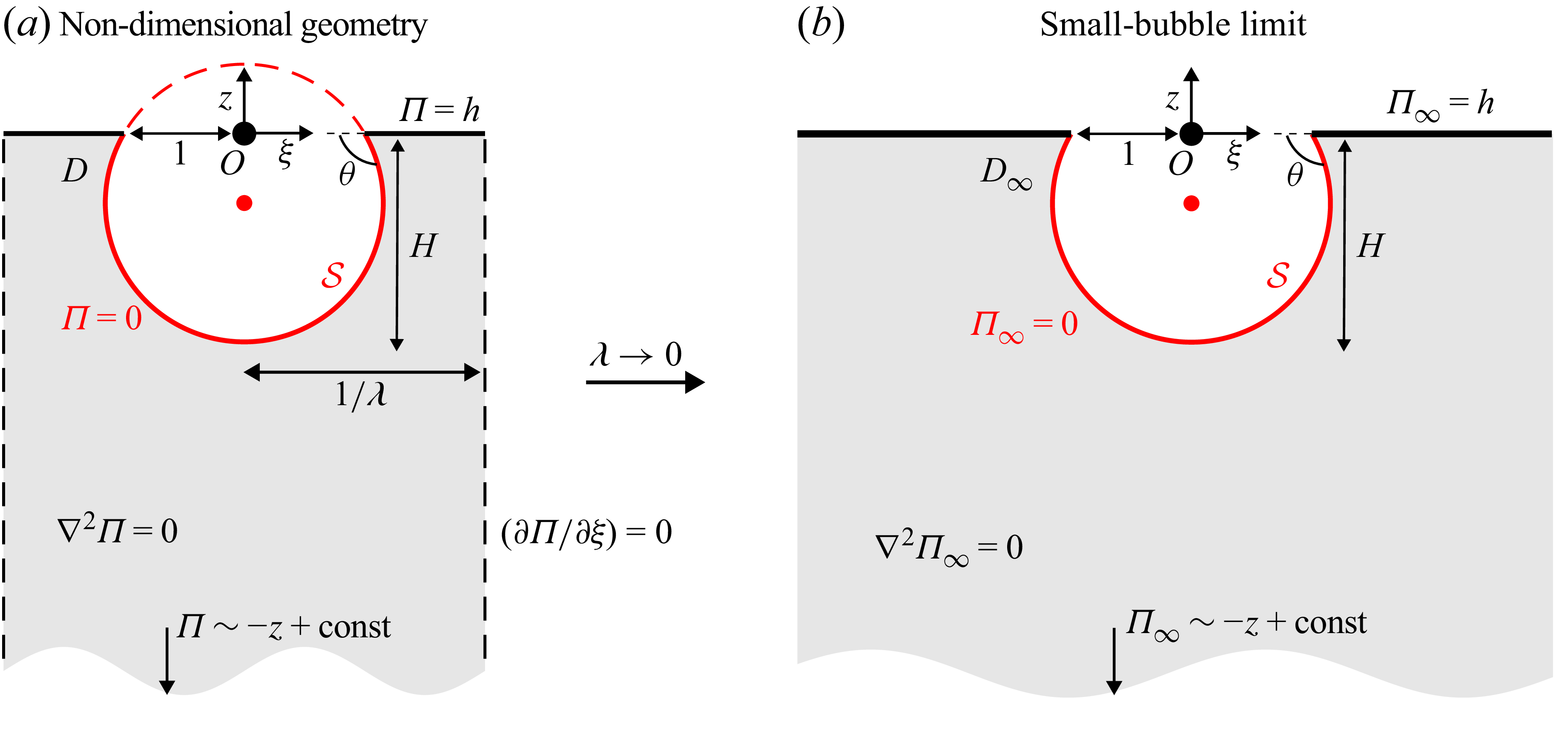The non-dimensional geometry is shown in figure 2(a).

Assuming axial symmetry of the shape of the cavity and container, it is convenient to study the jet speed in a cylindrical coordinate system defined by $(\xi ,z)$ . We consider a general solution to the 3-D potential problem in a cylindrical region outside of a spherical cavity. The boundary of a spherical bubble with a contact angle $\theta$ is defined as

(2.4) \begin{align} \mathcal{S} := \left \{(\xi ,z)\,\Bigg| \, \xi ^2 + \left (z - \frac {1}{\tan \theta } \right )^2 = \frac {1}{\sin ^2 \theta },\ z\leqslant 0 \right \}\!. \end{align}

Note that the depth of a bubble defined by $H$ is related to the contact angle $\theta$ by

(2.5) \begin{align} H = \tan (\theta /2). \end{align}

We assume that the container length in the $z$ -direction is much greater than the radius of the tube and the container. Hence the elastic collision on the bottom gives a uniform velocity distribution at $z\rightarrow -\infty$ after the impact.

The boundary condition for the interface is the Euler–Bernoulli equation at the free interface, which reduces to $\varPi =0$ on the meniscus $\mathcal{S}$ , and on the top of the liquid interface in the container at $1\lt \xi \lt 1/\lambda$ , $z=h$ (Onuki et al. Reference Onuki, Oi and Tagawa2018; Gordillo et al. Reference Gordillo, Onuki and Tagawa2020). Furthermore, assuming that the uniform gradient of the pressure impulse appears in the region above the bubble region, it is possible to approximate that the pressure impulse satisfies $\varPi =h$ on $z=0$ , $1\lt \xi \lt 1/\lambda$ . This assumption originates from the leading-order contribution to the pressure impulse $\varPi$ from the surface on $z=h$ , which is approximately constant and equal to $\varPi = h$ , even in the vicinity of $\xi = 1$ and for $\theta \gt \pi /2$ . This approximation was also adopted in previous work by Onuki et al. (Reference Onuki, Oi and Tagawa2018), where it was shown to be in good agreement with experimental results for predicting jet velocities. For the side of the container, an impermeability condition is imposed, i.e. $\partial \varPi /\partial \xi = 0$ for $\xi = 1/\lambda$ , $z\lt 0$ , as the movement of the container is assumed to be only along the $z$ -axis. As a result, the non-dimensional pressure impulse $\varPi$ satisfies the following mixed boundary value problem in cylindrical coordinates:

(2.6) \begin{align} \left \{ \begin{aligned} \textrm {(i)}\quad &{\nabla} ^{2} \varPi = 0,\quad &&(\xi ,z) \in D,\\[4pt]\textrm {(ii)}\quad &\frac {\partial \varPi }{\partial \xi }(1/\lambda ,z) = 0,\quad &&z\lt 0,\\[4pt]\textrm {(iii)}\quad &\varPi (\xi ,z)=0,\quad &&(\xi ,z)\in \mathcal{S},\\[4pt]\textrm {(iv)}\quad &\varPi (\xi ,0) =h,\quad &&1\leqslant \xi \leqslant 1/\lambda ,\\[4pt]\textrm {(v)}\quad & \varPi (\xi ,z) = -z + \textrm {const},\quad &&z \rightarrow -\infty , \end{aligned} \right . \end{align}

where the region $D$ is the fluid region for $z\lt 0$ , as shown in figure 2(a). After obtaining $\varPi$ , the initial jet speed is calculated using the velocity at the bottom of the cavity with respect to the moving frame with (2.2).

Figure 2.

(a) The non-dimensional boundary value problem for a harmonic pressure impulse $\varPi$ . (b) The geometry $D_\infty$ in the small-bubble limit. When $\lambda \rightarrow 0$ , the geometry is a semi-infinite half 3-D space outside a spherical-shaped bubble, denoted by $D_\infty$ . Note that $H$ is related to $\theta$ as $H = \tan (\theta /2)$ . The impulse $\varPi$ is approximated well by $\varPi _\infty$ as $\lambda \rightarrow 0$ .

3. The small-bubble limit

This section studies the small-bubble limit, i.e. when the cavity is sufficiently small compared to the radius of the container shown in figure 2(a). This case corresponds to the ratio of the radius of the inner tube to that of the container tending to $0$ , i.e. $\lambda \rightarrow 0$ . The region is now a semi-infinite lower-half 3-D region outside the spherical bubble $\mathcal{S}$ , denoted by $D_\infty$ . For this limiting case, it is possible to obtain an analytical solution for the field $\varPi _\infty$ and thus the jet velocity induced by the impulsive acceleration.

As $\lambda \rightarrow 0$ , the impermeability condition on the side wall in (2.6)(ii) vanishes. The pressure impulse defined by $\varPi _{\infty }(\xi ,z)$ now satisfies

(3.1) \begin{align} \left \{ \begin{aligned} \textrm {(i)}\quad &{\nabla} ^2 \varPi _{\infty } = 0,\quad && (\xi ,z) \in D_\infty ,\\[4pt]\textrm {(iii)}\quad &\varPi _{\infty }(\xi ,z)=0,\quad && (\xi ,z)\in \mathcal{S},\\[4pt]\textrm {(iv)}\quad &\varPi _{\infty }(\xi ,0) =h,\quad && 1\leqslant \xi \leqslant \infty ,\\[4pt]\textrm {(v)}\quad & \varPi _{\infty }(\xi ,z) = - z + \textrm {const},\quad && z \rightarrow -\infty . \end{aligned} \right . \end{align}

Figure 3.

Toroidal coordinates $(\alpha ,\beta )$ for solving the mixed boundary value problem for a pressure impulse $\varPi _\infty$ . Cylindrical coordinates $(\xi ,z)$ are mapped to the new coordinates $(\alpha ,\beta )$ using the transformation in (3.2). The boundary of the bubble is expressed by $\beta =\pi +\theta$ .

To solve the boundary value problem (3.1), it is convenient to change the cylindrical coordinates $(\xi ,z)$ to toroidal coordinates $(\alpha ,\beta )$ (Lebedev Reference Lebedev1965), where all boundaries of $D_\infty$ can be expressed by a contour line in this coordinate system. Following a mathematical setting provided in Chapter 8 of Lebedev (Reference Lebedev1965), consider the change of variables

(3.2) \begin{align} \xi (\alpha ,\beta )=\frac {\sinh \alpha }{\cosh \alpha -\cos \beta },\quad z(\alpha ,\beta )=\frac {\sin \beta }{\cosh \alpha -\cos \beta }, \end{align}

where the parameter spaces for $\alpha$ and $\beta$ in the domain $D_\infty$ are $0 \lt \alpha \lt \infty ,\ \pi +\theta \lt \beta \lt 2\pi$ . The inverse transform is given by

(3.3) \begin{align} \alpha (\xi ,z) = \frac {1}{2}\log \left (\frac {z^2 + (\xi + 1)^2}{z^2 + (\xi - 1)^2} \right ),\quad \beta (\xi ,z)= \pi +\tan ^{-1}\left (\frac {2z}{\xi ^2 + z^2 - 1} \right ), \end{align}

where $\beta$ is chosen so that $\pi +\theta \lt \beta \lt 2\pi$ . Using this coordinate system, the boundary of a spherical bubble $\mathcal{S}$ and the plane $1\lt \xi$ with $z=0$ correspond to $\beta =\pi + \theta$ and $\beta = 2\pi$ , respectively. The correspondence between the geometry and parameters $\alpha$ and $\beta$ is shown in figure 3. Using the new coordinates and the mathematical formulation in Lebedev (Reference Lebedev1965), the solution $\varPi _\infty (\xi ,z)$ for the boundary value problem (3.1) is given by

(3.4) \begin{align} \varPi _{\infty }(\xi ,z) = \varPi_{\kern-1pt f}(\xi ,z)+ h \varPi _g(\xi ,z), \end{align}

where

(3.5) \begin{align} &\varPi_{\kern-1pt f}(\xi ,z) := -z - f_\theta (\alpha (\xi ,z),\beta (\xi ,z)), \\[-12pt] \nonumber \end{align}

(3.6) \begin{align} &\varPi _g(\xi ,z) := 1- g_\theta (\alpha (\xi ,z),\beta (\xi ,z)), \\[10pt] \nonumber \end{align}

and

(3.7) \begin{align} f_\theta (\alpha ,\beta ) &:= 2\sqrt {2(\cosh \alpha - \cos \beta )}\int _0^\infty \tau \frac {\sinh (\theta \tau ) \sinh [(2\pi -\beta )\tau ] }{\cosh (\pi \tau ) \sinh [(\pi -\theta )\tau ] }P_{-({1}/{2}) + \textrm {i}\tau }(\cosh \alpha )\,{\textrm {d}} \tau , \\[-12pt] \nonumber \end{align}

(3.8) \begin{align} g_\theta (\alpha ,\beta ) &:= \sqrt {2(\cosh \alpha - \cos \beta )}\int _0^\infty \frac {\cosh (\theta \tau ) \sinh [(2\pi -\beta )\tau ] }{\cosh (\pi \tau ) \sinh [(\pi -\theta )\tau ] }P_{-({1}/{2}) + \textrm {i}\tau }(\cosh \alpha )\,{\textrm {d}} \tau . \\[10pt] \nonumber \end{align}

The cylindrical coordinates $(\xi ,z)$ are related to $(\alpha ,\beta )$ through the coordinate transformation (3.2). The function $P_\nu (z)$ is a special function called a Legendre function of the first kind with degree $\nu$ . The derivation of this formula is provided in detail in Appendix A.

Note that $\varPi_{\kern-1pt f}(\xi ,z)$ is a pressure impulse induced by the curvature of the spherical bubble with no submersion, and $\varPi _g$ is a pressure impulse induced by the submersion of the tube. The total pressure impulse $\varPi _\infty$ is decomposed into $\varPi_{\kern-1pt f}$ and $\varPi _g$ times the submersion length $h$ .

Although the expressions (3.7) and (3.8) are similar to (8.12.12) in Lebedev (Reference Lebedev1965), these solutions are novel due to the differing boundary conditions (i), (iii)–(v). This is also one of the main contributions of this paper.

This formula includes an integral of the function $P_{-({1}/{2}) + \textrm {i}\tau }(\cosh \alpha )$ with respect to $\tau$ . It is possible to calculate the function using some well-known integral representations (Lebedev Reference Lebedev1965). Numerical computations for this function in our paper are given in Appendix B.

The speed of the jet is calculated directly using the derivative of $\varPi _\infty$ in (3.4) with respect to $z$ evaluated at the bottom of the bubble. To achieve this, the derivatives of $f_\theta$ and $g_\theta$ are calculated using the chain rule:

(3.9) \begin{align} \frac {\partial f_\theta }{\partial z} = \frac {\partial \alpha }{\partial z}\frac {\partial f_\theta }{\partial \alpha } + \frac {\partial \beta }{\partial z}\frac {\partial f_\theta }{\partial \beta },\quad \frac {\partial g_\theta }{\partial z} = \frac {\partial \alpha }{\partial z}\frac {\partial g_\theta }{\partial \alpha } + \frac {\partial \beta }{\partial z}\frac {\partial g_\theta }{\partial \beta }. \end{align}

The jet speed is evaluated at the bottom of the spherical bubble located at $(\xi ,z)=(0,-H)$ . The parameters there are $\alpha =0$ and $\beta = \pi + \theta$ . Note that the derivatives of $f_\theta$ and $g_\theta$ with respect to $\alpha$ and $\beta$ in (3.9) can be explicitly evaluated. For example, the derivative of $g_\theta$ with respect to $\beta$ is given by

(3.10) \begin{align} \frac {\partial g_\theta }{\partial \beta } &= \frac {\sin \beta }{ \sqrt {2(\cosh \alpha - \cos \beta )}}\int _{0}^\infty \frac {\cosh (\theta \tau ) \sinh [(2\pi -\beta )\tau ] }{\cosh (\pi \tau ) \sinh [(\pi -\theta )\tau ] }P_{-({1}/{2}) + \textrm {i}\tau }(\cosh \alpha )\,{\textrm {d}} \tau \nonumber \\[5pt]&\quad{}-\sqrt {2(\cosh \alpha - \cos \beta )}\int _0^\infty \tau \frac {\cosh (\theta \tau ) \cosh [(2\pi -\beta )\tau ] }{\cosh (\pi \tau ) \sinh [(\pi -\theta )\tau ] }P_{-({1}/{2}) + \textrm {i}\tau }(\cosh \alpha )\,{\textrm {d}} \tau . \end{align}

By using the Mehler–Fock theorem and the integral representation of a Legendre function (Lebedev Reference Lebedev1965), the speed at the bottom of the cavity $v_f(\theta )$ in a frame moving with the tube is given explicitly by

(3.11) \begin{align} v_f(\theta ) := \frac {\partial f_\theta }{\partial z}(0,\pi +\theta ) = \sin ^2 \left (\frac {\theta }{2} \right ) + 8 \cos ^3\left (\frac {\theta }{2}\right )\int _0^{\infty } \tau ^2 \frac {\sinh (\theta \tau ) \cosh [(\pi -\theta )\tau ]}{\cosh (\pi \tau ) \sinh [(\pi -\theta )\tau ]}\,{\textrm {d}} \tau \end{align}

and

(3.12) \begin{align} v_g(\theta ):=\frac {\partial g_\theta }{\partial z}(0,\pi +\theta ) =\frac {1}{2}\sin \theta + 4\cos ^{3}\left (\frac {\theta }{2}\right )\int _0^\infty \tau \frac {\cosh (\theta \tau ) \cosh [(\pi -\theta )\tau ] }{\cosh (\pi \tau ) \sinh [(\pi -\theta )\tau ] }\,{\textrm {d}} \tau . \end{align}

Based on the pressure impulse decomposition (3.4), the total jet velocity $v(\theta )$ is then equal to

(3.13) \begin{align} v(\theta ) = v_f(\theta ) + h\, v_g(\theta ), \end{align}

which means that the velocity is composed of the velocity $v_f(\theta )$ due to the pressure impulse of the impact with $h=0$ , and the velocity $v_g(\theta )$ caused by the pressure distribution due to the submergence of the tube. This is natural since the solution (3.4) is composed of the hydrostatic pressure impulse due to the bubble $\varPi_{\kern-1pt f}$ and the pressure due to the submergence of the tube, which is $\varPi _g$ times the height $h$ . This decomposition is important because the jet speed $v(\theta )$ has a local maximum with respect to the bubble height $H=\tan (\theta /2)$ for fixed $h\gt 0$ .

Figure 4.

Contour plots for the harmonic pressure impulse $\varPi_{\kern-1pt f}(\xi ,z)$ in (3.5) and the velocity in (3.11), for (a) $H=0.4$ and (b) $H=1.5$ . The value $H$ is related to the angle $\theta$ as $H = \tan (\theta /2)$ .

Figure 4. Long description

Panel A: The left contour plot shows the harmonic pressure impulse for H equals 0.4. The horizontal axis is labeled xi ranging from -2 to 2, and the vertical axis is labeled z ranging from -2 to 0. The color gradient indicates pressure values from 0 to 2. The right plot shows the corresponding velocity field with arrows indicating direction and magnitude, and a red curve outlining a specific boundary. Panel B: The left contour plot shows the harmonic pressure impulse for H equals 1.5. The horizontal axis is labeled xi ranging from -2 to 2, and the vertical axis is labeled z ranging from -2 to 0. The color gradient indicates pressure values from 0 to 2. The right plot shows the corresponding velocity field with arrows indicating direction and magnitude, and a red curve outlining a specific boundary.

The final integrals in (3.11) and (3.12) do not appear to admit a simpler closed-form expression. However, since the integrand rapidly decays to zero as $\tau \rightarrow \infty$ , they can be readily evaluated numerically. Nonetheless, it is possible to show that for $\theta =\pi /2$ , the integral expression (3.11) can be simplified as follows:

(3.14) \begin{align} v_f(\pi /2) = \frac {1}{2} + 2\sqrt {2}\int _0^{\infty }\tau ^2\frac {\cosh \left (\dfrac{\pi }{2} \tau \right )}{\cosh (\pi \tau )}\,{\textrm {d}} \tau = 2. \end{align}

This result corresponds to figure 6 in Antkowiak et al. (Reference Antkowiak, Bremond, Le Dizès and Villermaux2007) as $\lambda \rightarrow 0$ , where the jet produced from hemispherical bubbles was studied. This velocity is consistent with the fact that the pressure impulse for $H=1$ ( $\theta =\pi /2$ ) is explicitly written as $\varPi_{\kern-1pt f}(\xi ,z) = -z - z/(\xi ^2 + z^2)^{3/2}$ . It is easy to see that the function satisfies $\varPi_{\kern-1pt f}(\xi ,z)=0$ on the lower hemisphere and $z=0$ , $\xi \geqslant 1$ . This fact will be used in § 4. For $\theta =0$ , it is easy to see that $v_f(0)=0$ and

(3.15) \begin{align} v_g(0) = 4\int _{0}^\infty \frac {\tau\, {\textrm {d}} \tau }{\sinh (\pi \tau )} = 8\int _0^\infty \frac {\tau\, {\textrm {d}} \tau }{{\rm e}^{\pi \tau } - {\rm e}^{-\pi \tau }} = 8 \lim _{\epsilon \rightarrow 0^+} \int _{\epsilon }^\infty \frac {\tau }{{\rm e}^{\pi \tau }}\sum _{n=0}^\infty {\rm e}^{-2n\pi \tau }\,{\textrm {d}} \tau = 1. \end{align}

Figure 4 shows contour plots of $\varPi_{\kern-1pt f}$ and velocity plots with cavity heights $H=0.4$ and $1.5$ . Note that $H$ and $\theta$ are related to each other by (2.5). As the cavity height $H$ increases, the magnitude of the velocity increases. It can also be observed that the maximum velocity is attained at the bottom of the bubble. This is natural because the spherical bubble pushes as $H$ increases, and the interval between contour lines becomes small, so that the pressure gradient at the bottom becomes large. For $h\gt 0$ , the contour plots of $\varPi _\infty$ and velocity plots for cavity height $H=1.5$ with $h=1$ and $2.5$ are shown in figure 5. The velocity becomes large as $h$ increases.

Figure 5.

Contour plots for the harmonic pressure impulse $\varPi _\infty (\xi ,z)$ in (3.4) and velocity in (3.13). Note that $\varPi _\infty (\pm 1,0)$ is discontinuous due to the boundary conditions. Here, (a) $h=1.0$ and (b) $h=2.5$ . The cavity height is fixed at $H=1.5$ .

Figure 6.

(a) The speed at the bottom of the bubble with different submersion depths $h$ . The jet velocities with four different $h$ values are examined, i.e. $h=0, 2.0, 4.0, 8.0$ . The circles correspond to the points where the velocity $v(\theta )$ is maximised. (b) The critical value of $H$ that maximises the jet speed with respect to the depth $h$ .

Figure 6. Long description

Panel A: A line graph shows the speed at the bottom of the bubble with different submersion depths. The x-axis represents bubble height H, and the y-axis represents jet velocity v(theta). Four different submersion depths are examined: h = 0, h = 2.0, h = 4.0, and h = 8.0. The lines are color-coded: black for h = 0, red for h = 2.0, magenta for h = 4.0, and blue for h = 8.0. Circles mark the points where the velocity is maximized for each submersion depth. Panel B: A line graph shows the critical value of bubble height H that maximizes the jet speed with respect to the depth h. The x-axis represents depth h, and the y-axis represents bubble height H. The graph shows a decreasing trend in H as h increases.

Figure 6 shows the jet velocity $v(\theta )$ with respect to $H=\tan (\theta /2)$ for different submersion depths, $h=0, 2.0, 4.0, 8.0$ . For $h=0$ , the velocity monotonically increases as the height of the bubble $H$ increases. On the contrary, for $h\gt 0$ , there exists a critical value of $H$ that maximises the velocity $v(\theta )$ . It is also observed that the critical value of $H$ gets smaller as $h$ increases.

As shown in figure 6(b), the critical bubble height $H$ converges as $h\rightarrow \infty$ . According to the velocity decomposition (3.13),

(3.16) \begin{align} v(\theta ) = v_f(\theta ) + h\,v_g(\theta ) \sim h\, v_g(\theta ) \end{align}

as $h$ becomes large. This means that the bubble height that maximises $v(\theta )$ is obtained by maximising $v_g(\theta )$ . Based on our numerical calculation, the value $H$ converges to $H\sim 0.67$ as $h\rightarrow \infty$ .

The formulas derived here work only when the walls and inner cavity are widely separated. When they are close, the jet velocity is not approximated well by the small-bubble limit. However, we will show that (3.7) and (3.8) are in good agreement with a wide range of parameter spaces of $\lambda$ and $H$ in the next section.

4. Exact solution for the pressure impulse using a series solution

Section 3 presents an analytical formula for the pressure impulse field and velocity when the bubble size is small enough to neglect the side wall effect. Although analytical formulas for the fields and velocities of liquid jets have been presented, the presence of the wall affects both. Antkowiak et al. (Reference Antkowiak, Bremond, Le Dizès and Villermaux2007) studied the relationship between the jet velocity and changes in the cavity size and tube radius, where the contact angle of the cavity is always $\pi /2$ . It was found, both numerically and experimentally, that the jet velocity decreases as the cavity approaches the wall boundary, i.e. $\lambda \rightarrow 1$ . It was also observed that the velocity in the $h=0$ case is approximately $1$ .

To study a situation similar to that in Antkowiak et al. (Reference Antkowiak, Bremond, Le Dizès and Villermaux2007), we present a semi-analytical approach for obtaining the pressure impulse in the presence of a wall boundary based on the analytical formulas in § 3. Similar to the formulation in Antkowiak et al. (Reference Antkowiak, Bremond, Le Dizès and Villermaux2007), the field inside the tube outside the spherical bubble is given by the superposition of high-order fields derived from the pressure impulse of (3.7) and (3.8).

4.1. Derivation of the semi-analytical solution for $\theta =\pi /2$ by Antkowiak et al.

Antkowiak et al. (Reference Antkowiak, Bremond, Le Dizès and Villermaux2007) derived a semi-analytical solution for a potential problem in a tube outside a hemispherical bubble, i.e. $\theta =\pi /2$ . They started the formulation by considering the initial function

(4.1) \begin{align} \phi _0(\xi ,z) := \frac {z}{(\xi ^2 + z^2)^{3/2}}. \end{align}

It is easy to see that $\varPi (\xi ,z):=-z - \phi _0(\xi ,z)$ satisfies the conditions (i), (iii)–(v) in (2.6). We consider the modified field $F_{0}(\xi ,z) := \phi _0(\xi ,z) + \psi _0(\xi ,z)$ , where $\psi _0(\xi ,z)$ is added to satisfy the boundary condition (ii). By employing the condition $\psi _0(\xi ,z)=0$ on $z=0$ , $\psi _0(\xi ,z)$ is represented by Fourier–sine functions with Bessel functions $I_0(\xi )$ as

(4.2) \begin{align} \psi _0(\xi ,z) := \int _{0}^\infty \eta _0(m)\sin (mz)\, I_0(m\xi )\, {\textrm {d}} m, \end{align}

where $\eta _0(m)$ is calculated from the Fourier–sine transform of the function to satisfy the boundary condition on the side wall of the tube:

(4.3) \begin{align} \eta _0(m) = -\frac {2}{\pi }\int _{-\infty }^0 \frac {\sin m z}{m\, I_1(m/\lambda )} \frac {\partial \phi _0}{\partial \xi }(1/\lambda ,z)\,{\textrm {d}} z. \end{align}

Although $-z - F_0(\xi ,z)$ is not an exact solution for the boundary value problem with a tube as $-z-F_0(\xi ,z)\neq 0$ on $\mathcal{S}$ , it is possible to obtain the solution using a new basis related to $\phi _0(\xi ,z)$ . Consider an even-number derivative of $\phi _0(\xi ,z)$ with respect to $z$ :

(4.4) \begin{align} \phi _{2n}(\xi ,z) : = \frac {1}{(2n)!}\frac {\partial ^{2n} \phi _0}{\partial z^{2n}}(\xi ,z),\quad \psi _{2n}(\xi ,z) :=\int _{0}^\infty \eta _{2n}(m)\sin (mz)\, I_0(m\xi )\, {\textrm {d}} m, \end{align}

where the coefficient $\eta _{2n}(m)$ is also calculated in a similar manner to (4.3) by simply modifying $\phi _{0}(1/\lambda ,z)$ as $\phi _{2n}(1/\lambda ,z)$ . The solution $\varPi (\xi ,z)$ is the superposition of the functions $F_{2n}$ :

(4.5) \begin{align} \varPi (\xi ,z) := -z - \sum _{n=0}^\infty A_{2n}\, F_{2n}(\xi ,z),\quad F_{2n}(\xi ,z) := \phi _{2n}(\xi ,z) + \psi _{2n}(\xi ,z). \end{align}

Antkowiak et al. (Reference Antkowiak, Bremond, Le Dizès and Villermaux2007) derived an explicit representation for $F_{2n}(\xi ,z)$ and then a linear system for the coefficients $A_{2n}$ , with truncation order $N$ .

We show that this approach is applicable to problems that do not always have a hemispherical bubble. The only modification is the basis function $\phi _{2n}$ .

4.2. A semi-analytical solution for an arbitrary angle $\theta$

We start the formulation from the solution $\phi _0(\alpha ,\beta ):=f_\theta (\alpha ,\beta )$ defined in (3.7). Note that this function is harmonic and satisfies $ \phi _0(\alpha ,\beta )=0$ for $\beta =2\pi$ . Similar to the definition of a new candidate function in (4.4), we define a harmonic function that is related to the $2n$ th derivatives of $\phi _0(\alpha ,\beta )$ with respect to $\beta$ , given by

(4.6) \begin{align} \phi _{2n}(\alpha ,\beta ) :=& \frac {2\sqrt {2(\cosh \alpha - \cos \beta )}}{(2n)!}\frac {\partial ^{2n}}{\partial \beta ^{2n}} \int _{0}^\infty \tau \frac {\sinh (\theta \tau )\sinh [(2\pi -\beta )\tau ]}{\cosh (\pi \tau ) \sinh [(\pi -\theta )\tau ]}P_{-(1/2)+\textrm {i}\tau }(\cosh \alpha )\,{\textrm {d}} \tau \nonumber \\[5pt]=&\frac {2\sqrt {2(\cosh \alpha - \cos \beta )}}{(2n)!} \int _{0}^\infty \tau ^{2n+1} \frac {\sinh (\theta \tau )\sinh [(2\pi -\beta )\tau ]}{\cosh (\pi \tau ) \sinh [(\pi -\theta )\tau ]}P_{-(1/2)+\textrm {i}\tau }(\cosh \alpha )\,{\textrm {d}} \tau , \end{align}

for $n=0,1,\ldots$ . These functions are harmonic in the domain $D$ and $\phi _{2n}(\alpha ,2\pi )=0$ , i.e. $\phi _{2n}(\alpha ,\beta )=0$ for $z=0$ , $\xi \geqslant 1$ in a cylindrical coordinate system. Using the new function $\phi _{2n}(\alpha ,\beta )$ and a correction function $\psi _{2n}(\alpha ,\beta )$ defined in (4.2) with a different kernel,

(4.7) \begin{align} \eta _{2n}(m) = -\frac {2}{\pi }\int _{-\infty }^0 \frac {\sin (mz)}{m\,I_1(m/\lambda )}\frac {\partial \phi _{2n}}{\partial \xi }(\alpha (1/\lambda ,z),\beta (1/\lambda ,z))\, {\textrm {d}} z, \end{align}

the solution for $\varPi (\xi ,z)$ is given by the superposition of $F_{2n}(\xi ,z) := \phi _{2n}(\alpha (\xi ,z),\beta (\xi ,z)) + \psi _{2n}(\alpha (\xi ,z),\beta (\xi ,z))$ :

(4.8) \begin{align} \varPi (\xi ,z) = -z - \sum _{n=0}^\infty A_{2n}\, F_{2n}(\xi ,z). \end{align}

This expression is similar to (4.5) by Antkowiak et al. (Reference Antkowiak, Bremond, Le Dizès and Villermaux2007), except for the different basis functions $F_{2n}(\xi ,z)$ . The coefficients $A_{2n}$ are determined so that $\varPi (\xi ,z)=0$ on $\mathcal{S}$ . After obtaining the coefficients $A_{2n}$ using a collocation method, it is possible to calculate the jet speed. This can be done by considering a derivative with respect to $z$ and the chain rule.

Figure 7 shows contour plots of $F_0(\xi ,z)$ , $F_{2}(\xi ,z)$ and $F_{4}(\xi ,z)$ for $\lambda = 0.5$ and $H=1.5$ . It can be seen that the higher-order oscillating terms can be included by adding $F_{2n}(\xi ,z)$ with a large $n$ . Through a linear combination of $F_{2n}$ , it is possible to extract the solution $\varPi$ for the boundary value problem (2.6).

Figure 7.

Contour plots of (a) $F_0(\xi ,z)$ , (b) $F_2(\xi ,z)$ and (c) $F_4(\xi ,z)$ for $\lambda = 1/2$ . Using the superposition of these functions, a solution that satisfies (i)–(v) is constructed.

4.3. A semi-analytical solution for a submerged tube

The same approach can be used to obtain the solution for the problem (2.6) with $h\neq 0$ . First, note that $g_\theta (\alpha ,\beta )$ defined in (3.8) does not satisfy the boundary condition on the side of the container. To satisfy the boundary condition, we consider a correction term $\tilde {\phi }_0(\alpha ,\beta ):= g_\theta (\alpha ,\beta )$ , and define

(4.9) \begin{align} G(\xi ,z) := \tilde {\phi }_0(\alpha (\xi ,z),\beta (\xi ,z)) + \tilde {\psi }(\alpha (\xi ,z),\beta (\xi ,z)), \end{align}

where $\tilde {\psi }(\xi ,z)$ is given by (4.2) in terms of a Fourier–sine series of $\tilde {\phi }_0(\xi ,z)$ . Using that, the pressure field is given by

(4.10) \begin{align} \varPi (\xi ,z) = -z - \sum _{n=0}^\infty \tilde {A}_{2n}\, F_{2n}(\xi ,z) + h\left (1-G(\xi ,z)\right ), \end{align}

where the final term captures the boundary condition at $z=0$ and singularities at $z=0$ , $\xi =\pm 1$ . After finding the coefficients $\tilde {A}_{2n}$ , it is possible to evaluate the field and velocity of the jets.

For the numerical computation, we truncate the series (4.8) at $N$ to calculate the velocity of jets $v(\theta )$ at the bottom of the bubble. Due to the suitability of the basis in the mixed boundary value problem, the required number of basis functions is small. Similarly to Antkowiak et al. (Reference Antkowiak, Bremond, Le Dizès and Villermaux2007), we find that approximately 5–10 bases are sufficient for condition (iv), and absolute error $10^{-4}$ is obtained. In this paper, eight basis functions are used in all computations. The same number of collocation points is chosen on half of $\mathcal{S}$ to construct the linear system for $A_{2n}$ or $\tilde {A}_{2n}$ to satisfy the boundary condition (iii) in (2.6).

Figure 8 compares the analytical solutions (3.11) and (3.12) for the small-bubble limit, plotted as a black dashed line, and the numerical solutions approximated as a series of basis functions. The accuracy of the analytical solution for the small-bubble limit improves as $\lambda$ and $h$ decrease. These numerical results indicate that the approximation of the analytical solution derived in (3.11) and (3.12) works well for a wide range of $\lambda$ and $h$ , especially for small $\lambda$ and $h$ .

Figure 8.

A comparison between the analytical solutions (3.11) and (3.12) for the small-bubble limit plotted as a black dashed line and the numerical solutions calculated as a series of basis functions, for (a) $H=0.8$ and (b) $H=1.5$ , with $h=0,1,2,4$ . It can be seen that the accuracy of the analytical solution of the small-bubble limit becomes good as $\lambda$ and $h$ decrease. The error between the analytical solutions (black dashed lines) and the full solutions (coloured lines) is less than $0.2\,\%$ for $H=0.8$ , and less than $0.6\,\%$ for $H=1.5$ , when $\lambda = 0.074$ .

Figure 8. Long description

Two line graphs compare analytical and numerical solutions for jet velocity in different scenarios. Panel A: The line graph shows jet velocity (v) on the vertical axis and lambda (λ) on the horizontal axis for H equals 0.8. The black dashed line represents the small bubble limit, while colored lines represent numerical solutions for different values of h (0, 1, 2, 4). Panel B: The line graph shows jet velocity (v) on the vertical axis and lambda (λ) on the horizontal axis for H equals 1.5. Similar to Panel A, the black dashed line represents the small bubble limit, and colored lines represent numerical solutions for different values of h (0, 1, 2, 4). The legend indicates the values of h corresponding to each colored line.

Figure 9.

A schematic of the experimental set-up. A container with an inserted capillary tube is fixed above a steel substrate using an electromagnet, and the container is released by switching off the electromagnet to impact the steel substrate. The depth of the bubble $H^*$ is varied by adjusting the pressure inside the capillary tube using a syringe. The bubble and the jet are recorded using a high-speed camera.

5. Experiment

This section describes the experimental set-up adopted in this work, and compares the experimental results with analytical formulas. The trends of the experimental results are approximated well by the analytical results, i.e. there exists an optimal value to produce high-velocity jets, as shown in figure 6.

5.1. Experimental set-up

To produce liquid jets, we follow the example of previous works by Kiyama et al. (Reference Kiyama, Tagawa, Ando and Kameda2016) and Onuki et al. (Reference Onuki, Oi and Tagawa2018), who studied impulse-driven liquid jets produced in a free-falling container. The experimental set-up is shown in figure 9. A test tube (IWAKI, 30 $\times$ 200) with inner radius $r^*=13.5$ mm is filled with silicone oil (Shin-Etsu Silicones, KF-96 series) of kinematic viscosity 10 $\textrm {mm}^2\ \textrm{s}^{-1}$ and density 932 $\textrm {kg}\,\textrm {m}^{-3}$ . Silicone oil has a low vapour pressure and is less prone to cavitation, which makes it possible to suppress cavitation-induced effects and isolate the effects of bubble depth and curvature on jet velocity. A glass capillary tube with inner radius $R^*=1$ mm is inserted into the test tube and firmly fixed using a capillary holder fabricated with a 3-D printer (Bambu Lab A1 3-D printer). A syringe (Terumo, SS-20LZ) is used to connect the container to a small tube, then the bubble is injected into the top of the tube. A steel S-shaped hook is attached to the top of the capillary holder, and the container is suspended above a steel base plate using an electromagnet (Eclipse Magnetics, M52180-12VDC). The distance between the base plate (Toshin Steel, material SS400, thickness $\times$ width $\times$ length are $20\times 150 \times 150\ \text{mm}^3$ ) and the bottom of the container is 20 mm. When the electromagnet is switched off, the container undergoes free fall and collides with the base plate. Upon impact, the liquid in the container is rapidly accelerated, ejecting a focused jet from an air bubble at the lower end of the capillary. A high-speed camera (Photron, FASTCAM SA-X, 10 000–40 000 fps) with a backlighting set-up (PHLOX, white LED backlight 400 $\times$ 200 mm²) is used to record the behaviour of the bubble during the free fall of the container, as well as the jet formation process. The parameter $\lambda$ , which is the ratio of the radius of the tube to the radius of the container outside the tube, is $0.074$ in all experiments. For this $\lambda$ , it was possible to approximate the jet velocity using the analytical formulas (3.11) and (3.12), as shown in figure 8. The depth of the viscous liquid is set to $60$ mm, which is assumed to be much larger than the tube radius. The Reynolds and Weber numbers are calculated using the capillary radius ( $1$ mm) as the characteristic length scale, and the jet velocity as the characteristic velocity. The resulting values are listed in table 1.

Table 1.

The Reynolds number and Weber number in our experiment.

Table 1. Long description

A table comparing Reynolds and Weber numbers for different values of h. The table has three rows and two columns. The rows are labeled with h values: h = 0, h = 2, and h = 4. The columns are labeled Re and We. Row 1: h = 0, Re = 1.11 x 10^2 - 8.68 x 10^2, We = 5.70 x 10^1 - 3.49 x 10^3. Row 2: h = 2, Re = 4.47 x 10^2 - 1.43 x 10^3, We = 9.25 x 10^2 - 9.52 x 10^3. Row 3: h = 4, Re = 1.09 x 10^3 - 3.13 x 10^3, We = 5.45 x 10^3 - 4.54 x 10^4.

Note that the Weber numbers are found to lie in the range $5.70\times 10^1$ – $4.54\times 10^4$ , with the smallest value still corresponding to ${We} \gg 1$ . Following the argument of Gekle & Gordillo (Reference Gekle and Gordillo2010), capillary effects are expected to be subdominant during the initial jet formation. Therefore, treating surface tension as a secondary effect in the pressure impulse model is justified for the present parameter range. Nevertheless, surface tension and viscosity may still contribute to the subsequent jet development.

The experimental parameters are $h^*$ and $H^*$ . Three values of $h^*$ are examined: $h^*=0,2,4$ mm, which are set based on visual inspection. As $H^*$ oscillates while the tube is falling, a video is captured using a horizontally placed camera. The value of $H^*$ immediately before impact is determined from the recorded images by visual inspection and subsequent analysis using ImageJ. The position of the jet tip generated just after impact is also identified visually, and the jet velocity is then calculated. Experiments are conducted to measure the jet speed as a function of the bubble height $H^*$ and submersion depth $h^*$ .

Figure 10.

Image sequences of the jet. The moment of impact between the container and the substrate is defined as $t = 0$ ms. For each condition, six images are shown, including images taken before the container is released and 25 ms before impact. The yellow triangles indicate the jet tip position. The bubble grows as the container falls, and becomes nearly spherical. For $h = 0$ , the jet velocity increases with increasing $H$ . In contrast, for $h \gt 0$ , there exists a value of $H$ at which the jet velocity reaches a maximum, and this value depends on $h$ . For $h = 2$ , the jet velocity is maximised at $H = 1.56$ , while for $h = 4$ , it reaches a maximum at $H = 1.37$ . The positions and velocities of the gas–liquid interface centre are plotted in the bottom panel. A frame rate of $40\,000$ fps is used for $h=0$ , and $10\,000$ fps is used for $h=2$ and $h=4$ . The red lines show the velocity $U_\theta ^*(h)$ , which is compared with our model given by (3.11) and (3.12).

5.2. A comparison of the analytical solution with experimental results

Figure 10 shows image sequences of the jet with different $h=h^*/R^*$ and $H=H^*/R^*$ . We set $t=0$ as the time when the container collided with the base. The jet formation process is shown at time intervals 1 ms for $h=0$ , 0.5 ms for $h=2$ , and 0.3 ms for $h=4$ . For each condition, the image sequences in figure 10 also include the spherical bubble shape before the container is released, as well as that during the free fall of the container (25 ms before impact). For $h=0$ and $h=2$ , the bubbles are partially hidden by the interface, making their shapes difficult to observe. Under all conditions, the bubble approaches a nearly spherical, laterally symmetric shape during the free fall of the container. Subsequently, when the container impacts the base plate, the bubble undergoes significant deformation, leading to the ejection of a focused jet. Focusing on the jet tip position at $t=3$ ms for $h=0$ , it is observed that the jet tip height increases with increasing $H$ . This indicates that for $h=0$ , the jet velocity increases as $H$ increases. In contrast, for $h\gt 0$ , a larger value of $H$ does not necessarily lead to a higher jet tip position. For $h=2$ , the jet tip position at $t=1.5$ ms shows that the maximum jet height is obtained at $H=1.56$ . Similarly, for $h=4$ , the jet tip position at $t=0.9$ ms reaches its maximum at $H=1.37$ . These results suggest that for $h\gt 0$ , there exists an optimal value of $H$ at which the jet velocity is maximised, and that this optimal value depends on $h$ .

We calculate the average jet velocity of two time instants, $t_0$ and $t_1$ . Time $t_0$ is defined as the moment when the jet tip first forms, while $t_1$ corresponds to the time at which the jet reaches its maximum observable length within the camera view. The jet tip’s positions are measured at these two time points, and the average jet velocity $U_\theta ^*(h)$ is then determined from their displacement. The positions and the measured velocity $U_\theta ^*(h)$ of the jet tip are shown at the bottom of figure 10.

To fit our analytical solution with the experimental data, we first non-dimensionalised the measured velocity $U_\theta ^*(h)$ using the velocity of the container $U_0^*$ just after impact:

(5.1) \begin{align} U_{\theta }(h) := \frac {U_{\theta }^*(h)- U_0^*}{U_0^*}. \end{align}

The container experiences free fall before the elastic impact at the bottom. The container velocity $U_0^*$ is given by $\sqrt {2g^*a^*}$ , where $a^*$ represents the container drop height fixed at $20$ mm for all experiments, and $g^*$ is the gravitational acceleration. The resulting velocity is $U_0^*=0.6241$ m s⁻¹.

Note that our model provides a pressure-impulse-induced initial velocity soon after impact, which differs from the average jet-tip velocity measured in the experiment. To compare the analytical solutions with the experimental data, we considered the following scaling factor $\gamma (h)$ , which depends only on the height $h$ :

(5.2) \begin{align} U_{\theta }(h) \approx \gamma (h)\, (v_f(\theta ) + h\, v_g(\theta )). \end{align}

The scaling factor represents a physical correction that captures the difference between our model and the measured velocity. The reason why we introduce $\gamma (h)$ is explained in § 6. The value $\gamma (h)$ is determined through fitting of the experimental data using the least squares method. The values of $\gamma (h)$ are $3.143$ at $h=0$ , $3.918$ at $h=2$ , and $5.615$ at $h=4$ .

Figure 11.

A comparison between the analytical solution for the small-bubble limit in (3.11) and (3.12), plotted as solid lines, and the experimental data, plotted as dots. The ranges of measured jet velocity $U_\theta ^*$ are $1.11{-}8.68$ m s⁻¹ for $h=0$ , $4.47{-}14.33$ m s⁻¹ for $h=2$ , and $10.85{-}31.30$ m s⁻¹ for $h=4$ . The data are non-dimensionalised by the velocity of the container $U_0^*=0.6241$ m s⁻¹, and plotted for $h=0, 2.0, 4.0$ . Black circles correspond to the maximum jet velocity in both our theoretical and experimental results. When measuring $U_\theta ^*(h)$ , experimental uncertainties arise from errors of a few (approximately 3) pixels when identifying the jet tip at two time instances. The corresponding uncertainties for $h=0,2,4$ are also shown. Black dashed lines correspond to the full solution results (4.10) with $\lambda =0.074$ for $h=2.0, 4.0$ . The full solution is well approximated by the analytical solutions in (3.11) and (3.12).

Figure 11. Long description

Panel A: A line graph shows the relationship between the normalized jet velocity (Uθ - U0)/U0* and the normalized cavity height H. The x-axis represents the normalized cavity height H, and the y-axis represents the normalized jet velocity. Three solid lines represent different values of h (0, 2.0, and 4.0), and a black dashed line represents the full solution. Data points are plotted as dots with error bars. The graph shows that the jet velocity increases with the cavity height up to a certain point and then decreases. Panel B: A photograph shows a liquid jet formed by impulsive forcing. The jet is emanating from a cavity at the bottom of a container. The photograph includes labels for the jet radius R* and the cavity height h*.

Figure 11 compares the analytical solution for the small-bubble limit in (3.11) and (3.12), plotted as solid lines, and the experimental data, plotted as dots. Both experimental and analytical data are plotted for $h=0,2.0,4.0$ . Each black circle corresponds to a maximum jet velocity in our experiments. Note that when measuring $U_\theta ^*(h)$ , experimental uncertainties arise from errors of a few (approximately 3) pixels when identifying the jet tip at two time instances. The corresponding uncertainties for $h=0,2,4$ are also shown in figure 11. Although a scaling factor $\gamma (h)$ is needed to fit the experimental data, the trend of the experimental data is approximated well by the analytical solution $v(\theta )$ . This indicates that controlling the bubble height $H$ and the submersion depth $h$ is important for producing a high-velocity jet.

7. Summary

This work has established an expanded analytical framework for the formation of impulse-driven jets from curved fluid interfaces. By solving the pressure impulse problem for spherical bubbles with arbitrary contact angles, we have shown that the jet velocity is governed by the competition between curvature-induced impulse focusing and submersion-induced pressure redistribution. This competition gives rise to an optimal interface geometry that maximises jet speed, providing a clear physical explanation for experimentally observed non-monotonic trends.

Beyond the specific configuration considered here, the present formulation offers a foundation for systematically exploring impulse focusing in more general axisymmetric geometries. The ability to relate interface curvature directly to jet velocity opens a pathway to geometry-controlled jet engineering, such as conical interfaces, with potential implications for high-speed microjet generation, flow focusing devices, and impact-driven injection technologies.