INTRODUCTION
The total area of maize (Zea mays L.) grown in Canada in 2011 was 1·63 million ha, which is nearly double the area in 1971 (0·92 million ha). Approximately 0·80 (i.e. 1·3 million ha) is grown for grain, with Ontario and Quebec growing 0·60 and 0·30 of the areas of grain maize, respectively (Statistics Canada 2014). Maize grain yield, presented in dry matter hereafter, increased from 4000 kg/ha in 1961 to 8000 kg/ha in 2010 in North America (FAO 2014). It has been estimated that 0·50–0·60 of yield increases are related to genetic improvement and the remainder to management improvement such as increased synthetic fertilizer application and increased plant density (Cardwell Reference Cardwell1982; Duvick Reference Duvick2005b ). Based on the results obtained from the field experiments that maize cultivars from different eras were grown at plant densities from 1 to 7·9 plants/m2, the yields of the 1930s cultivars showed no significant difference among densities. The yields of cultivars from the 1990s were similar to those from the 1930s at low density, but increased significantly at high densities (Tollenaar & Lee Reference Tollenaar and Lee2002). This showed that the yield increase from the 1930s to the 1990s may have been the result of an improved interaction between cultivar and density management, since maize planting density increased gradually from the 1930s to the 1990s (Duvick Reference Duvick2005a ). With economic development and urbanization, staple diets have shifted to diets containing increased shares of livestock products in developing countries (Wirsenius et al. Reference Wirsenius, Azar and Berndes2010). The increasing demand for maize grain as feed requires increasing yield. In turn, it is necessary to recognize the limiting factors for further yield improvement in maize production regions, including Eastern Canada.
Increases in maize yield from 1961 to 1990 were associated with increased fertilizer use, with nitrogen (N) fertilizer being a driver for significant yield improvements since 1960 (Cassman et al. Reference Cassman, Dobermann, Walters and Yang2003). Producers in Ontario usually apply higher rates than that required by the crop, as a management measure against the risk of yield loss (Rajsic & Weersink Reference Rajsic and Weersink2008). An 8-year experiment in Ottawa, Eastern Canada revealed that the yield gap between no N application and sufficient N applications (up to 250 kg N/ha) was often <2000 kg/ha (Subedi & Ma Reference Subedi and Ma2009). This yield gap was >3000 kg/ha in Nebraska, USA (Cassman et al. Reference Cassman, Dobermann, Walters and Yang2003). The varied yield gaps between N strategies may have been a result of different cultivars and environmental conditions. In particular, soil N supply, related to soil type and weather conditions (Dobermann et al. Reference Dobermann, Witt, Abdulrachman, Gines, Nagarajan, Son, Tan, Wang, Chien, Thoa, Phung, Stalin, Muthukrishnan, Ravi, Babu, Simbahan, Adviento and Bartolome2003), influenced crop yield response to applied fertilizer N. Gabrielle et al. (Reference Gabrielle, Da-Silveira, Houot and Michelin2005) reported that N mineralization ranged from 12 to 82 kg N/ha/year for wheat–maize rotation systems, and the N losses related to soil initial mineral N. Nyiraneza et al. (Reference Nyiraneza, Ziadi, Zebarth, Sharifi, Burton, Drury, Bittman and Grant2012) showed that the soil N supply in maize field is 76 ± 47·9 kg/ha in Eastern Canada. Therefore, it is helpful to understand the causes of yield gaps by assessing yield response of different cultivars to fertilizer N strategies under different environments with varied soil types. A quantifying approach governing the cultivar–soil–climate interaction system is required to help assess the yield response to biotic and abiotic factors in Eastern Canada.
Grain yield potential (YP) of maize appears to be stable, based on field experiments conducted over recent decades (Duvick Reference Duvick, Edmeades, Bänziger, Mickelson and Pena-Valdivia1997, Reference Duvick2005b ). In those experiments, YP was measured by growing maize plants under conditions of negligible competition for resources such as incident radiation, soil nutrients and soil moisture. Maize yields as high as 19 600 kg/ha were reported in the Northern USA in the 1970s (Nelson & Reetz Reference Nelson and Reetz1986) and similar high yields were recorded in Canada in the 1990s (Tollenaar & Lee Reference Tollenaar and Lee2002). In these cases, crop management practices were favourable to maintain sufficient water and nutrient supplies and to minimize the stress from weeds, insects and diseases. These recorded high yields mostly depended on cultivar type, solar radiation and temperature, and they were taken as YP for the specific cultivars in the specific environment. Apparently, the harvested yields are often much lower than their genetic potential because of local environments and management practices that may not ideally meet the requirements of the cultivar. In some countries, YP predicted by models such as CERES serves as a target for crop management, linked to appropriate rates of N inputs (Van Wart et al. Reference Van Wart, Kersebaum, Peng, Milner and Cassman2013). However, reports identifying the barriers to narrow the gap between actual and potential yield of maize in Eastern Canada are scarce. Additionally, recognized yields from actual to potential levels in Canada can also provide essential information for assessing future food and feed issues (Wirsenius et al. Reference Wirsenius, Azar and Berndes2010). Focusing on the interactions of cultivar, environment and management offers the best way of narrowing the yield gap by using water and nutrients more efficiently (Hatfield & Walthall Reference Hatfield and Walthall2015). Crop growth models quantifying the cultivar–environment–management processes provide a useful tool for quantitative analysis on the adaptability of a cultivar to climatic conditions and facilitate exploration of options to reduce the gap between actual and potential yields. Those options include selecting/designing cultivars for certain soil and climatic conditions under prescribed water and nutrient management inputs (Jackson et al. Reference Jackson, Robertson, Cooper and Hammer1996; Yan & Hunt Reference Yan and Hunt1998).
Crop modelling offers an alternative to field experiments for assessing the potential benefits of cultivar selection and crop management by analysing traits with computer-based experiments across a number of locations, soil types and growing seasons. To carry out such simulation experiments, a model needs to be comprehensive and must take into consideration the dynamics of crop–soil–weather interactions. There are many models/model groups that simulate crop–soil–weather systems, such as STICS (Simulateur mulTIdisciplinaire pour les Cultures Standard, Brisson et al. Reference Brisson, Gary, Justes, Roche, Mary, Ripoche, Zimmer, Sierra, Bertuzzi, Burger, Bussière, Cabidoche, Cellier, Debaeke, Gaudillère, Hénault, Maraux, Seguin and Sinoquet2003), APSIM (Agricultural Production Systems sIMulator, Keating et al. Reference Keating, Carberry, Hammer, Probert, Robertson, Holzworth, Huth, Hargreaves, Meinke, Hochman, McLean, Verburg, Snow, Dimes, Silburn, Wang, Brown, Bristow, Asseng, Chapman, McCown, Freebairn and Smith2003), DSSAT (Decision Support System for Agrotechnology Transfer, Jones et al. Reference Jones, Hoogenboom, Porter, Boote, Batchelor, Hunt, Wilkens, Singh, Gijsman and Ritchie2003), CropSyst (Cropping Systems simulation model, Stöckle et al. Reference Stöckle, Donatelli and Nelson2003) and the Wageningen crop models (Van Ittersum et al. Reference Van Ittersum, Leffelaar, Van Keulen, Kropff, Bastiaans and Goudriaan2003). One crop models widely used around the world to simulate crop–environment systems is CSM–CERES (Crop System Model–Crop Environment Resource Synthesis; Richie & Otter Reference Ritchie and Otter1985; Jones & Kiniry Reference Jones and Kiniry1986) within DSSAT. The CSM–CERES–Maize model has been evaluated recently for soil water and N cycles in maize fields in Southern Ontario (Liu et al. Reference Liu, Yang, Drury, Reynolds, Tan, Bai, He, Jin and Hoogenboom2011a , Reference Liu, Yang, Tan, Drury, Reynolds, Zhang, Bai, Jin, He and Hoogenboom b , Reference Liu, Yang, Drury, Liu and Reynolds2014). In these studies, maize yields under water- and N-limited conditions were evaluated; however, the model has not been applied to analyse the YP and yield gap in Eastern Canada. The current study aimed to expand the adaption and application of the CSM–CERES–Maize model in Eastern Canada and furthermore to use it as a tool to analyse factors affecting crop production.
The objective of the present study was to assess the gaps between potential and actual yields in order to identify management options to improve production of grain maize. The assessment was based on modelling the interactions of cultivar, environment and management in Eastern Canada. The CSM–CERES–Maize model in DSSAT v4·6 (Hoogenboom et al. Reference Hoogenboom, Jones, Wilkens, Porter, Boote, Hunt, Singh, Lizaso, White, Uryasev, Ogoshi, Koo, Shelia and Tsuji2015) was first calibrated and evaluated with maize experimental data before its application in the assessment. The calibrated model was used to simulate maize yield levels defined as potential, water- and N-limited yields. Subsequently, yield gaps associated with water and N deficiencies were analysed and options to narrow the yield gaps suggested.
MATERIALS AND METHODS
Field experiments
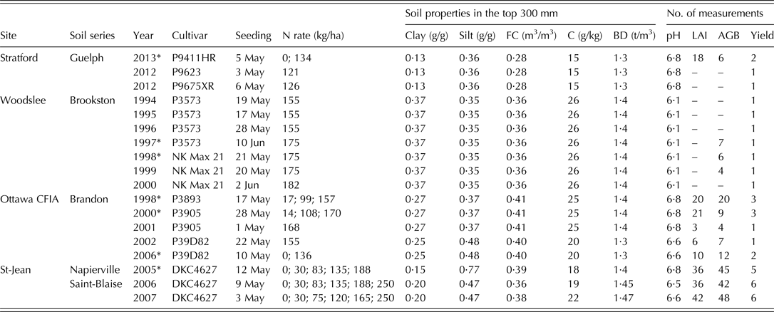
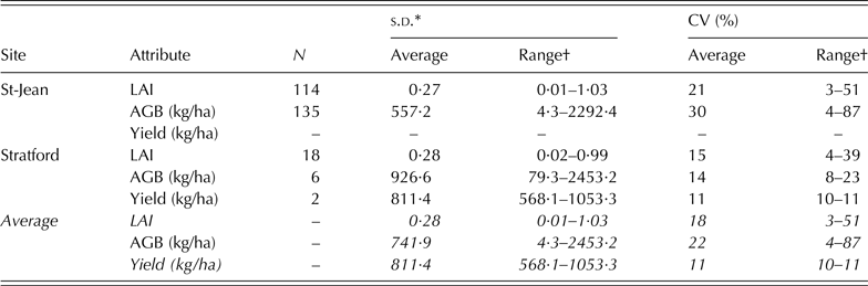
Field experiments were conducted at Stratford, Woodslee and Ottawa in Ontario and at Saint-Jean-sur-Richelieu (St-Jean hereafter) in Quebec in Eastern Canada for various studies, such as optimization of fertilizer applications and using remote sensing to monitor crop growth conditions (Fig. 1 and Table 1). At each site, a randomized complete block design with three or four replications was used. These experiments covered various soil types and fertilizer N application rates from 0 to 250 kg/ha without irrigation. Above-ground biomass (AGB) (dry matter) was measured using destructive sampling three to nine times during the maize growing season in the years shown in Table 1. The grain was harvested using a mechanical combine from which yields were determined. The standard deviation (s.d.) and coefficient of variation (CV) values of the measured data were calculated from the experimental data sets at St-Jean and Stratford (Table 2).
Locations of the field experimental sites on the ecozones map of Canada (AAFC 2015), together with the 30-year (1981–2010) averages of accumulated thermal time for maize (GDD, base temperature as 6 °C) and precipitation totals (Precip) from April 1 to October 31.

Summary information, soil properties and number of measurements taken in the four field experiments on cultivar and management

FC, field capacity; BD, bulk density; LAI, leaf area index; AGB, above-ground biomass.
* Calibration set; the remainder was used as an evaluation set.
Standard deviation (s.d.) and coefficient of variation (CV) of leaf area index (LAI), above-ground biomass (AGB) and grain yield; measured data in two experiments

N, number of means of measured data.
* With the same unit of its attribute.
† s.d. and CV values corresponding to a given site, year and sampling date.
At the Stratford site, cvar P9411HR was seeded in a tilled loam soil on 5 May 2013 at a depth of 40–50 mm to a density of 8·3 seeds/m2 with a row space of 0·76 m. The soil was prepared by strip tillage to a depth of 100–130 mm before seeding. Two rates of fertilizer N, 0 and 134 kg N/ha, were applied. At seeding, 131 kg N/ha 28% urea-ammonium nitrate (UAN) was broadcast and 3 kg N/ha liquid N 6-24-6 fertilizer was sprayed in the N treatment field. Herbicides Touchdown and Aatrex were applied once in mid-May and Touchdown alone once more in early June. Leaf area index (LAI) was measured in the field through canopy light interception using a LAI-2000 plant canopy analyser (Li-Cor, Lincoln, NE, USA). In 2012, cvar P9623 was seeded on 3 May and P9675XR on 6 May, with N fertilizer rates of 121 and 126 kg/ha, respectively. Liquid N 6-24-6 (equivalent to 3 kg N/ha) was sprayed and the remaining fertilizer N as 28% UAN was broadcast at seeding. Other management practices were similar to those in 2013.
At the Woodslee site two maize cultivars, P3573 and NK Max 21, were used in different years from 1994 to 2000. Maize was seeded in a Brookston clay loam soil (Orthic Humic Gleysol according to the Canadian System of Soil Classification, Evans & Cameron Reference Evans and Cameron1983). The seeding dates were 19 May 1994, 17 May 1995, 28 May 1996, 10 June 1997, 21 May 1998, 20 May 1999 and 2 June 2000. The soil was tilled at a depth of 180–200 mm before seeding. The seeding density was 7·1–7·8 seeds/m2. Nitrogen fertilizer was applied at seeding and top dressing at rates of 155, 175 and 182 kg N/ha (Table 1). Starter fertilizer (8-32-16) was applied with the seed (50 mm beside and 5 mm below the seed) to provide 20 kg N/ha. Nitrogen fertilizer (UAN 28%N) was also applied as side dressing when the maize was approximately at the six-leaf stage. The plot size was 20 m in length and 9 m in width. Maize was harvested in October and November. More detailed information can be found in Drury et al. (Reference Drury, Yang, Reynolds and McLaughlin2008).
At the Ottawa site, cvar P3893 was seeded on 17 May 1998, cvar P2905 was seeded on 28 May 2000 and 1 May 2001 and cvar P39D82 was seeded on 22 May 2002 and 10 May 2006. The seeding density ranged from 6·5 to 8 seeds/m2. The experiments were distributed in different plots with similar soil properties and each plot size was at least 100 × 50 m2. The N fertilizer rates ranged from 0 to 170 kg N/ha, applied at seeding as UAN (Table 1). Leaf area index was measured with a leaf area meter (LI-3100, Li-Cor, Lincoln, NE, USA). Maize was harvested in late October or November.
At the St-Jean site, cvar DKC4627 was used in the experiment. Maize crops were sown in three fields with different soils on 12 May 2005, 9 May 2006 and 3 May 2007 (Table 1). The seeding density was 7·9 seeds/m2 in 2005, 7·4 seeds/m2 in 2006 and 7·0 seeds/m2 in 2007. Plot size was 10 × 6 m2 and N fertilizer was applied at various rates from 0 to 250 kg N/ha. In the N treatments, 30 kg N/ha as calcium ammonium nitrate was surface broadcast at seeding and the rest as side dressing at the six-leaf stage. Leaf area index was measured with LAI-2000 (LI-COR, Lincoln, NE, USA). More information on field management and sampling can be found in Ziadi et al. (Reference Ziadi, Bélanger, Gastal, Claessens, Lemaire and Tremblay2009).
Weather data
Weather data including daily maximum and minimum temperature, solar radiation and total precipitation for the years of the experiment were measured near the experimental fields, except for the Stratford site. Weather data for the Stratford site were obtained from the Environment Canada (http://climate.weather.gc.ca) weather/climate stations (Stratford and Kitchener/Waterloo, 17·9–23·3 km east of the experimental site) and daily solar radiation was calculated using the method proposed by Allen et al. (Reference Allen, Pereira, Raes and Smith1998). These data were used for model calibration and evaluation.
Climate data used in the 30-year (1981–2010) long-term simulations for scenario analysis on maize yield were measured at meteorological stations close to the experimental sites for Ottawa and Woodslee. Because climate data for 1981–2010 were not available at Stratford and St-Jean, climate data from nearby Environment Canada stations in London, Ontario were used for Stratford and in Montreal, Quebec for St-Jean. In the cases where measured values were not available, solar radiation data were calculated by the same method noted above.
The CSM–CERES–Maize model
The module-based crop modelling package DSSAT (Jones et al. Reference Jones, Hoogenboom, Porter, Boote, Batchelor, Hunt, Wilkens, Singh, Gijsman and Ritchie2003; Hoogenboom et al. Reference Hoogenboom, Jones, Wilkens, Porter, Boote, Hunt, Singh, Lizaso, White, Uryasev, Ogoshi, Koo, Shelia and Tsuji2015) includes the individual plant growth model CSM–CERES for simulating wheat, maize, barley and some other crops (Jones & Kiniry Reference Jones and Kiniry1986). The model is described in detail by Jones et al. (Reference Jones, Hoogenboom, Porter, Boote, Batchelor, Hunt, Wilkens, Singh, Gijsman and Ritchie2003). Briefly, crop development is governed by thermal time, i.e. growing degree-days (GDD), which is computed based on daily temperature. Daily plant growth is computed by converting daily intercepted photosynthetically active radiation into plant biomass using crop-specific radiation use efficiency (RUE). Light interception is computed as a function of LAI, plant population and row spacing. Growth of new tissues depends on daily available carbohydrate and partitioning to different tissues as a function of phenological stage, which is modified by water deficit and N deficiency stress indices. Above-ground biomass has priority for partitioning carbohydrate and at the end of each day, carbohydrate not used for AGB is allocated to roots. However, roots must receive a specified stage-dependent minimum of the daily carbohydrate available for growth. Kernel numbers per plant are computed during flowering based on the cultivar's genetic potential, canopy weight, and average rate of carbohydrate accumulation during flowering, temperature, water and N stresses.
Daily demand for N is calculated from dry matter, growth rates and N concentrations of the plant organs. Critical and minimum N concentrations are calculated as the function of crop development stages. Actual crop N uptake is limited by maximum physiological uptake rate of the plant and by the maximum available amount of N in the soil. Vegetative N content is split into leaf and stem components. Leaf N concentration affects leaf photosynthesis rate and leaf expansion rate. When N supplies are insufficient, growth decreases due to reduced photosynthesis rate resulting from reduced leaf N concentration. This reduced growth leads to decreasing N demand until a new balance is reached between N demand and supply. The N supply includes soil initial inorganic N, mineralized N during crop growth and externally applied fertilizer N. In simulating crop growth with zero externally applied fertilizer N, soil initial N and mineralized N during crop growth supply the crops for their N demand. Therefore, inputs for soil initial N and soil properties are important for simulations under treatments with 0 N. The CERES-based soil carbon and N balance routines (NTRANS) in DSSAT (Godwin & Jones Reference Godwin, Jones, Hanks and Ritchie1991; Godwin & Singh Reference Godwin, Singh, Tsuji, Hoogenboom and Thornton1998) are based on the PAPRAN model (Seligman & Van Keulen Reference Seligman, Van Keulen, Frissel and Van Veen1981). Soil organic matter (SOM) is divided into different pools and the decomposition of SOM follows first-order kinetics. The transport of N as ammonium and nitrate N in each soil layer is associated with water flux obtained from the soil water module. Ammonia volatilization is simulated in the current version. The soil water balance model computes daily changes in soil water content of various soil layers as a result of infiltration of rainfall and irrigation, vertical drainage, unsaturated flow, soil evaporation, plant transpiration and root water uptake (Ritchie Reference Ritchie, Tsuji, Hoogenboom and Thornton1998). Potential transpiration is calculated by the Priestley–Taylor relationship (Priestley & Taylor Reference Priestley and Taylor1972). Actual transpiration is modified by LAI, soil evaporation and soil water. Water stress is calculated by potential and actual transpiration of the crop.
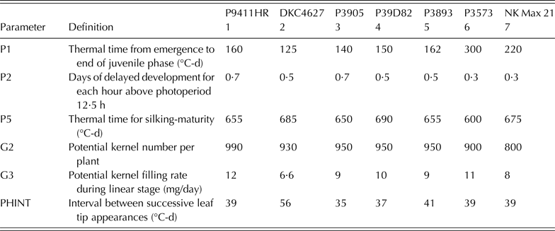
In order to run the CSM–CERES–Maize model, crop genetic parameters, soil initial conditions and crop management data are required. The genetic parameters recommended for cultivar calibration (Jones et al. Reference Jones, Hoogenboom, Porter, Boote, Batchelor, Hunt, Wilkens, Singh, Gijsman and Ritchie2003) are listed in Table 3. There are also numerous ecotype and species parameters in the model (Hoogenboom et al. Reference Hoogenboom, Jones, Wilkens, Porter, Boote, Hunt, Singh, Lizaso, White, Uryasev, Ogoshi, Koo, Shelia and Tsuji2015), such as parameters of plant N, plant RUE, specific leaf area, leaf senescence etc.; however, it is recommended to leave these parameters unchanged unless there are reliable data available for calibration. The minimum weather data required to drive the model include daily total incident solar radiation on the top of the crop canopy, maximum and minimum air temperature and precipitation.
Parameter definition and their calibrated values for each cultivar of maize used at the four sites in Eastern Canada

Model evaluation
The experimental data sets of seven cultivars at four sites in Eastern Canada were used to evaluate the model. The experimental data were divided into two separate sub-sets – a calibration set and an evaluation set (as marked in Table 1) at each site. The model was calibrated by tuning the parameters to match the simulated crop development and growth with the observed life cycles and values of LAI, AGB and grain yield. The calibrated parameters for each specific cultivar are presented in Table 3. The calibrated model was evaluated with the evaluation set at each site. In the evaluation procedure, the calibrated crop parameters at each site were used, and the simulated LAI, AGB and grain yield were compared with the measured values in the independent evaluation data set. The cultivars used at the Stratford site varied through years; and cvar P9411HR with dynamic data of LAI and biomass was used for calibration of crop parameters. Only grain yields were measured for the cvars P9623 and P9675XR in 2012. The model was evaluated with crop parameters of cvar P9411HR and the observed yields of cvars P9623 and P9675XR in 2012, as these cultivars are similar. At the Ottawa site, only cvar P3893 was calibrated due to the lack of additional independent data.
The simulated and measured values of LAI, AGB and yield were compared graphically. Model performance criteria were calculated following Bouman & Van Laar (Reference Bouman and van Laar2006): the slope (a), intercept (b) and coefficient of determination (R 2) for a linear regression between simulated Y(y 1, y 2,…,y i ,…,y n ) and measured X(x 1, x 2,…, x i,…, x n ) values; paired t test (P(t)); root-mean-squared errors (RMSE) and normalized root-mean-squared errors (nRMSE) between simulated and measured values, using Eqns (1) and (2):
 $$RMSE = {\left( {\displaystyle{{\sum {{{({Y_i} - {X_i})}^2}}} \over n}} \right)^{0 {\cdot} 5}}$$
 $$nRMSE = \displaystyle{{RMSE} \over {\bar X}}$$
where n is the number of observations and
 $\bar X$
is the average of measured values.
Model efficiency (EF), mean error (ME) and its relative value rME, and index of agreement (d) between simulated and measured values were also calculated from Eqns (3)–(6), after Beaudoin et al. (Reference Beaudoin, Launay, Sauboua, Ponsardin and Mary2008) and Yang et al. (Reference Yang, Yang, Liu and Hoogenboom2014).
 $$EF = 1 - \left( {\displaystyle{{\sum {{{({Y_i} - {X_i})}^2}}} \over {\sum {{{({X_i} - \bar X)}^2}}}}} \right)$$
 $$d = 1 - \displaystyle{{{{\sum {({Y_i} - {X_i})}} ^2}} \over {\sum {{{( \vert {Y_i} - \bar X \vert + \vert {X_i} - \bar X \vert )}^2}}}} $$
 $$ME = \displaystyle{1 \over n}\sum\nolimits_{i = 1}^n {({Y_i} - {X_i})} $$
 $$rME = \displaystyle{{ME} \over {\bar X}}$$
The model performance is acceptable if these statistics meet the following criteria: a close to 1·0, b close to 0, R 2 close to 1·0, P(t) > 0·05, RMSE similar to the s.d. of measured values, nRMSE similar to the CV of measured values, EF and d close to 1·0 and ME close to 0. In crop model evaluations, the nRMSE between simulated and observed attributes is generally deemed acceptable when it is <0·30 (Jamieson et al. Reference Jamieson, Porter and Wilson1991). Combinations of d ⩾ 0·75 and EF ⩾ 0 are considered acceptable for plant growth evaluation (Yang et al. Reference Yang, Yang, Liu and Hoogenboom2014).
Scenarios
The calibrated model was used to simulate four levels of grain yields with various cultivars, environments and management practices defined as: (1) yield potential (YP), i.e. maize yield is limited only by cultivar type, temperature and solar radiation without any other stresses; (2) water-limited yield (YW), i.e. maize yield is limited by natural water availability (rainfall) without N stresses; (3) water- and N-limited yield (YW, N) with a high N input (YW, N-160N), i.e. maize yield is under the water-limited scenario with a fertilizer application rate of 160 kg N/ha; and (4) water- and N-limited with a low N input (YW, N-80N), i.e. maize yield is under the water-limited scenario with a fertilizer application rate of 80 kg N/ha. The yield levels of YP, YW, YW, N and actual yield (YA) followed the concepts in Van Ittersum et al. (Reference van Ittersum, Cassman, Grassini, Wolf, Tittonell and Hochman2013). In simulation options, both N and water stresses were switched off for the simulation of YP, while only N stress was switched off for YW. In all these simulations, no impacts of weeds, diseases or physical crop damage were simulated. The two N rates, 80 and 160 kg/ha, mostly cover the range of N rates used by producers in the region depending on the expected yields (OMAFRA 2014). For simplicity in the simulations, N was only applied at seeding, although side dressing is a common practice in the region. Maize grain yields were simulated under these four scenarios for the 30-year period from 1981 to 2010 at four field experiment sites.
All the calibrated cultivars were used at each site to predict four yield levels, based on the assumption that these calibrated genetic coefficients are biophysical characteristics of the cultivars independent from their environments. The simulation results with multiple cultivars and sites facilitated analyses on the interaction between cultivars and environments. According to current local production practices, the seeding date in the simulations was fixed at 8 May for Stratford and Woodslee, and 15 May for Ottawa and St-Jean. The seeding density was set to 7·6 seeds/m2, as in the field experiments. The soil data measured in the field (Table 1) were used for initializing soil moisture in each year, where soil properties from the 1998 to 2001 experiments in Ottawa and soil properties from the 2006 experiment in St-Jean were used.
The statistical yield of 2003–2013 in the county where an experimental site was located was referred to as the YA relevant to the experimental site. These county-level yields were obtained as Montérégie Nord-Est region for St-Jean from ISQ (2015); Perth region for Stratford, Essex region for Woodslee and Ottawa region for Ottawa, respectively, from OMAFRA (2015). As the statistical county-level yield, YA, was averaged from the maize yields produced in all suitable soils across the county, it might be representative of the yield level at the experimental site but deviations should be expected. Three analyses were conducted to assess the sensitivity of the simulated yields to soils across the county, assuming climate is similar within the county. These three analyses were: (1) the measured yield in field experiments with N rates from 80 to 160 kg/ha was compared with its county YA at each site; (2) yields were simulated for a site and the county where it was located and these site- and county yields were compared; and (3) yield deviations due to various soils across a county were quantified. The Ottawa site and the ‘ecodistrict’ (equivalent to the county in area size) where the Ottawa site was located were selected to conduct the last two analyses. The yields were simulated from 1981 to 2010 using the calibrated model for the site and the region. The soil properties from the 1998 to 2001 experiments in Ottawa were used to simulate the site yield. Soil data for the ecodistrict were obtained from the Canadian Soil Information System (CanSIS) (MacDonald & Kloosterman Reference MacDonald and Kloosterman1984) and Soil Landscapes of Canada (SLC), version 3.2 (Soil Landscapes of Canada Working Group 2010), as described in Huffman et al. (Reference Huffman, Qian, De Jong, Liu, Wang, McConkey, Brierley and Yang2015). A total of 19 types of soils were retrieved from CanSIS for the selected ecodistrict. The weather data from 1981 to 2010 of the Ottawa site were used to simulate maize yields. The two cultivars P3905 and P39D82 used in the experiments at the Ottawa site were used in the simulations, with an N rate of 120 kg/ha (intermediate of the recommended rates in Ontario). Other management practices were the same as in scenario YW,N. The 30-year simulation was conducted for each cultivar grown in each of the 19 soil types, respectively. The 30-year average of the simulated yields for each cultivar was calculated for each soil type and CV of the yields among the soils across the ecodistrict was computed. The regional yield at the ecodistrict was calculated from the simulated yield in each soil and the area of each type of soil in the ecodistrict, using the upscaling method in Huffman et al. (Reference Huffman, Qian, De Jong, Liu, Wang, McConkey, Brierley and Yang2015).
The yield gaps were assessed between YP and YA. The factors related to water and N deficiencies were analysed by separating the gaps among simulated YP, YW, YW, N-160N and YW, N-80N. The yield gap assessment was associated with analysing interactions of cultivar and environment to explore management options. The analysis of variance (ANOVA) was performed on simulated yields using GenStat 17th Edition (Payne Reference Payne2014). The interactions between factors and contributions of each factor to yield variations were determined from Factor Analysis using GenStat. In the analysis, the factors included management, cultivar, location and year. Years were introduced to represent inter-annual climate variability.
RESULTS
Model evaluation
Values of the calibrated parameters varied among cultivars (Table 3). The crop parameters were generally related to vegetative growth (P1, P2 and PHINT) and reproductive growth (P5, G2 and G3). Parameters obtained from the calibration exercise revealed that the selected cultivars, although not exhaustive, included different genetic types with relatively different biophysical characteristics; for example, cvar DKC4627 with short juvenile phase v. P3573 with long juvenile phase, and low potential kernel number cvar NK Max 21 v. high kernel number P9411HR.
Leaf area index
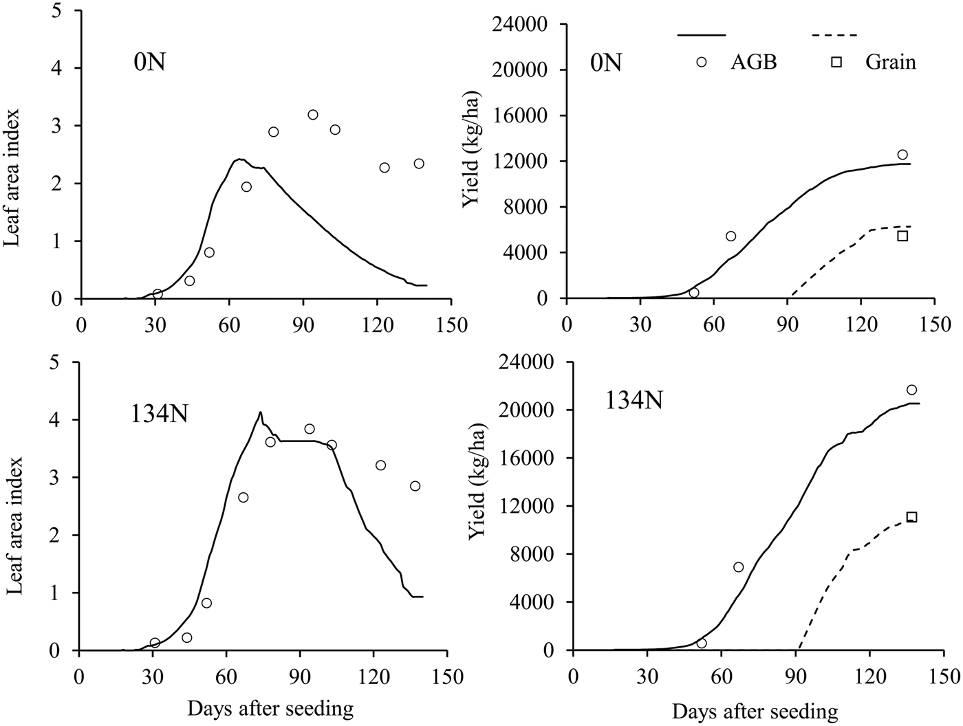
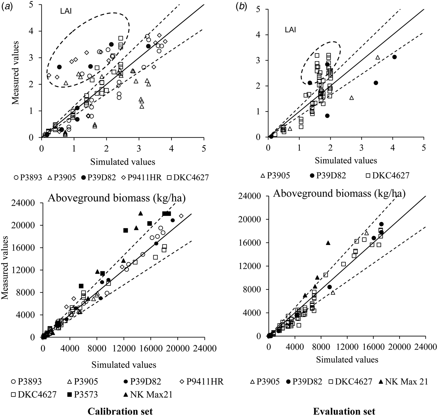
The model differentiated LAI under different fertilizer N rates, showing low LAI at 0 kg N/ha and high LAI at 134 kg N/ha at Stratford in 2013 (Fig. 2). The simulated LAI matched the measured values as LAI increased to its maximum at both N rates; however, LAI was underestimated as LAI declined during senescence. Comparing simulated and measured LAI with the 1 : 1 line showed that many points deviated from the 1 : 1 line and were >1 s.d. from the measured values (Fig. 3), showing a poor simulation of LAI with nRMSE > 0·38. A large portion of these simulation deviations were found during the LAI declining phase when the simulated values of LAI were lower than the measured values (data points within the ovals in Fig. 3).
Examples of dynamically simulated (lines) leaf area index (left panels), above-ground biomass (AGB) and grain biomass (right panels) v. measured (symbols) values of maize cultivar P9411HR at N rates of 0 and 134 kg/ha (0 and 134 N) at Stratford in 2013.

Simulated v. measured values of leaf area index (LAI) and above-ground biomass for calibration set (panel a) and evaluation set (panel b) from all experiments. Solid lines are the 1 : 1 relationship; dash lines are plus and minus the mean s.d. of measured values around the 1 : 1 line. Data are from different years, N application rates, and cultivars (see Table 1). The data points during the LAI declining phase are within the ovals in the panels for LAI.

Above-ground biomass
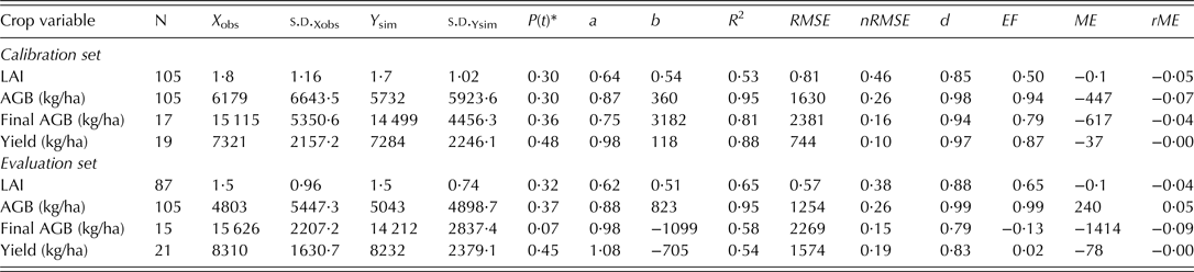
The simulated AGB agreed with the measured values for both fertilizer N rates at Stratford in 2013 (right panel, Fig. 2). Above-ground biomass was also successfully simulated at other sites. Most data points of AGB concentrated around the 1 : 1 line and within 1 s.d. of measured values for calibration and evaluation sets (lower panels, Fig. 3). No significant difference was found from the paired t test results. The differences between simulated and measured AGB were 447 and 240 kg/ha for calibration and evaluation sets (Table 4), only 0·07 and 0·05 of the measured average values, respectively. The EF was close to 1·0, and nRMSE was 0·26, comparable with the CV (22%) of measured values (Table 2).
Statistical criteria for evaluating simulations of leaf area index (LAI), above-ground biomass (AGB), final AGB and grain yield for the calibration and the evaluation sets

N, the number of measured/simulated data pairs; X obs mean of measured values; Y sim mean of simulated values; s.d. standard deviation; P(t) P-value from the paired t test; a slope of linear relation between simulated and measured values; b intercept of linear relation between simulated and measured values; R 2 coefficient of determination between simulated and measured values; RMSE root mean squared error between simulated and measured values; nRMSE normalized RMSE; d index of agreement; EF model efficiency; ME mean error and rME relative ME.
* Difference in the mean is considered statistically significant at P ⩽ 0·05 if the P-value is <0·05.
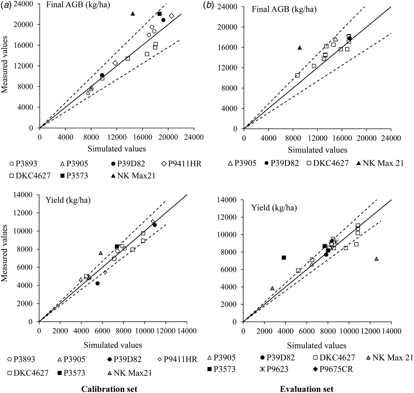
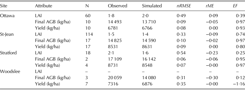
The final AGB was all of the AGB of the crop at physiological maturity. Most data points for final AGB were close to the 1 : 1 line in the comparison of simulated and measured values, and fell within 1 s.d. of the measured values (Fig. 4). Results from the paired t test (Table 4) showed that the mean of simulated final AGB was not significantly different from that of the measured values. The nRMSE in both calibration and evaluation was less than the CV (22%) of the measured value, suggested a satisfactory simulation for the final AGB in general. However, the final AGB was underestimated at Woodslee with rME = −0·30 (Table 5) and nRMSE of 0·31. The nRMSE (0·15) of final AGB for the evaluation set was smaller than that (0·16) for the calibration set, because the weight for the data from Woodslee was higher in the calibration set than the evaluation set (Table 1). The nRMSE at Woodslee was much greater than the nRMSEs at other sites (<0·10; Table 5).
Simulated v. measured final above-ground biomass (AGB) and grain yield for calibration set (a) and evaluation set (b) from all experiments. Solid lines are the 1 : 1 relationship; dash lines are plus and minus the mean s.d. of measured values around the 1 : 1 line. Data are from different years, N application rates, and cultivars (see Table 1).

Observed v. simulated means and their nRMSE, rME and EF on leaf area index (LAI), final above-ground biomass (final AGB) and grain yield at four sites

N, number of measured/simulated data pairs; nRMSE, normalized root mean squared error between simulated and measured values; EF, model efficiency; rME, relative mean error.
Grain yield
The simulated yields were close to the measured yields under zero and 134 kg N/ha at Stratford in 2013 (right panel, Fig. 2), indicating that the model captured yield variation due to varying N rates. Data points for grain yield were close to the 1 : 1 line on the scatter plot, with the majority of the data points being within 1 s.d. of measured data in the calibration set (Fig. 4). The average simulated yield was close to the average measured value and the nRMSE of 0·11 was comparable to the CV of measured values (Table 2) for the calibration set. For the evaluation set, most of the data points fell near the 1 : 1 line; however, discrepancies for cvar NK Max 21 at Woodslee were >1 s.d., showing less successful simulations. The nRMSE for yield over all experiments in the present study was 0·20, indicating overall good agreement between measured and simulated values. Among the four sites, maize grain yields were very well simulated at Ottawa, St-Jean, and Stratford with nRMSE <0·10, but were less successfully simulated at Woodslee with nRMSE > 0·30 (Table 5).
Simulated grain yields under the prescribed scenarios
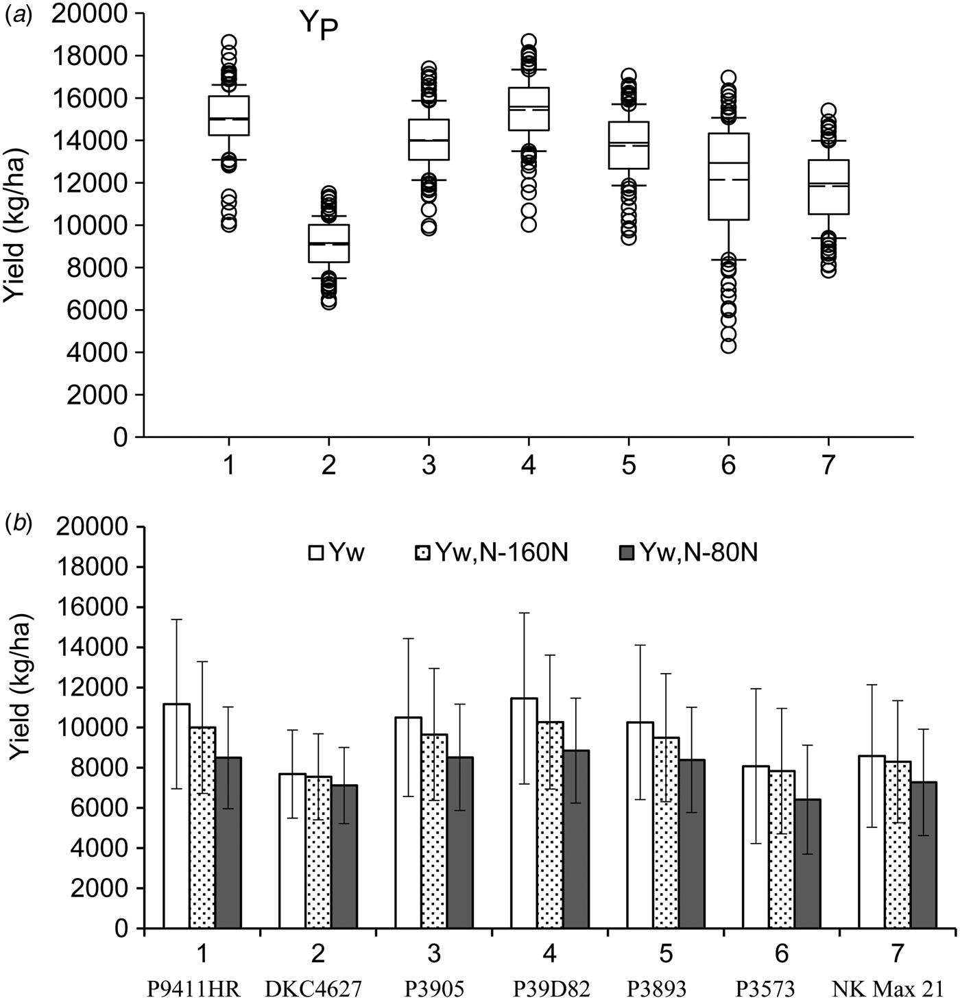
Simulated grain yields showed remarkable differences among the cultivars used in the experiments at each of four levels YP, YW, YW,N-160N and YW,N-80N (Fig. 5). The seven cultivars were divided into three grades according to the averages of YP. Cultivars P9411HR and P39D82 had a high YP, cvars DKC4627, P3573 and NK Max21 had a low YP, and cvars P3905 and P3893 had moderate YP. This yield trend among the cultivars was also investigated for YW. For YW,N-160N and YW,N-80N, cvars P9411HR and P39D82 with high Yp were comparable with cvars P3905 and P3893 with moderate Yp, and higher than the cultivars with low Yp. The YP difference between P9411HR and DKC4627 was about 6000 kg/ha, but this difference declined progressively through YW and YW,N-160N to about 1000 kg/ha at the YW,N-80N scenario. The declining grain yield differences among cultivars from YP to YW,N-80N indicated stronger tolerance of cultivars with a low YP to stress factors than those with a high YP. Furthermore, yields overlapped among cultivars due to their yield variations associated with environments (years and sites) at each production level. The highest YP was simulated for cvar P9411HR and P39D82 at >18 000 kg/ha.
Grain yield potential (YP) of seven cultivars demonstrated with box plots across four sites and 30 years, and comparison among water-limited yield (YW), water- and N-limited yields with 160 kg N/ha (YW, N-160N) and 80 kg N/ha (YW, N-80N). In (a), the boundary of the box closest to zero indicates the 25th percentile, the solid line within the box marks the median, the short dash line marks the mean, the boundary of the box farthest from zero indicates the 75th percentile, whiskers above and below the box indicate the 90th and 10th percentiles. In (b), whiskers on the bars are the s.d. across four sites and 30 years.

The cultivars with a high YP generally had a higher potential kernel number and relatively high potential kernel filling rate, with a medium juvenile period (Table 3). For the cultivars with a low YP, a lower potential kernel filling rate (DKC4627) and smaller kernel number (P3573 and NK Max 21) might be the major genetic characteristics limiting their yields.
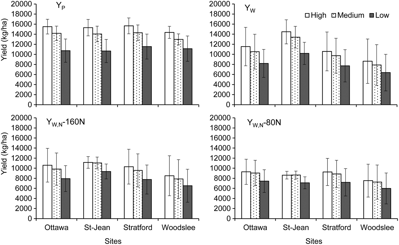
The average yields of cultivars with high and low YP were shown for the 30 years in Fig. 6 and for the four sites in Fig. 7, respectively. The grain yields of cultivars with medium YP were between these two types. A gap of 3000–4000 kg/ha between YW and YP was found for both low- and high-yield cultivars. Grain yield difference between the cultivars with high and low YP was about 6000 kg/ha without water and N stresses, 3000 kg/ha with only water stress, and 2000 kg/ha with water and N stresses (Fig. 6). This declining grain yield gap with the increasing stresses indicated a lower stress tolerance of the cultivars with high YP than those with low YP. The simulated grain yields showed a very large inter-annual variability, especially under rainfed conditions (YW, YW, N-160 and YW, N-80). The difference between the highest and the lowest years in the 30-year period was as large as 9000 kg/ha for YW and YW,N-160N (Fig. 6). This difference declined to <6000 kg/ha for the cultivars with a low YP. The average gap between YW and YW,N-80N was about 3000 kg/ha for cultivars with high YP, and only 1000 kg/ha for cultivars with low YP, indicating different responses to N stress between cultivar types.
Yearly yield variation for yield potential (YP), water-limited (YW), water- and N-limited with 160 kg N/ha (YW, N-160N) and with 80 kg N/ha (YW, N-80N). Whiskers are standard errors for the comparison between two types of cultivars with high and low yield potential (YP) across four sites during the 30 years (1981–2010).

Grain yield comparisons between three types of high, medium and low yield potentials among four sites for yield potential (YP), water-limited (YW), water- and N-limited with 160 kg N/ha (YW, N-160N) and with 80 kg N/ha (YW, N-80N). Whiskers on the bars refer to s.d..

The average values of YP at Ottawa, St-Jean and Stratford were slightly higher than at Woodslee for the cultivars with high and medium YP (Fig. 7), but they were similar among all four sites for the cultivars with low YP. The average YW was higher at St-Jean than the other three sites for all kinds of cultivars, indicating less water stress for maize at St-Jean than at other sites, even with similar precipitation among sites (Fig. 1). However, the average difference between the YW,N-160N and YW,N-80N was greatest at St-Jean, suggesting that maize suffered more from N stress at low N rates and implying the need for high N rates in the St-Jean area. Under water-limited conditions, grain yields were generally lower in Woodslee than at the other three sites.
From the analysis on yield variation due to different soils in an ecodistrict, the CV of simulated yields was 35% among all the different soils (Table 6). The yield variation among soils showed that the county yield might deviate from a site yield for a specific soil type, but this deviation was <0·35 of the county yield, on average. The simulated site yield was very close to the simulated county yield with a deviation of about 0·05. In addition, the measured yield at each experimental site was also close to its county yield YA. The deviations between county yield and measured site yield were 0·02–0·17 across the four sites. These deviations were comparable with the CV (11%) of measured yields in the experiments. These deviations between county and site yields indicated that it was reasonable to use the county yields to represent actual yields at the study sites for yield gap analysis.
The coefficient of variation (CV) of simulated yields among 19 soils across the ecodistrict where the Ottawa site was located, and comparisons between county- and site yields based on simulations and statistics/measurements, respectively

* Simulations were conducted with two cultivars in all soils across the ecodistrict under 120 kg N/ha from 1981 to 2010. Statistics/measurements refer to the statistical yield in each county where the experiment site was located and the measured average yield with N rate between 80 and 160 kg/ha at each experimental site.
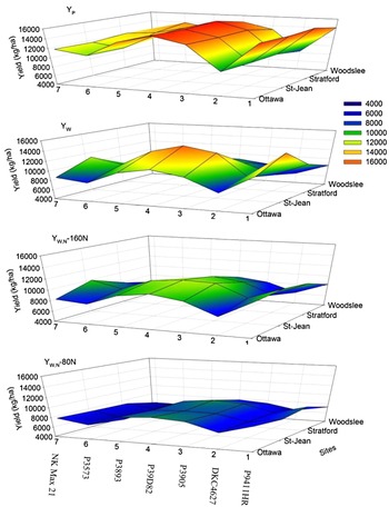
The interactions between sites and cultivars are shown in Fig. 8. The values of YP were more dependent on cultivar than site. Cultivars P9411HR and P39D82 had the highest average YP across years and DKC4627 the lowest. The uniformity of YP among sites disappeared under the scenarios of water-limited or water- and N-limited production. The YW values of cvars P9411HR and P39D82 were significantly (P < 0·05) greater at St-Jean than at other sites. This trend was not maintained for YW, N-80N. The YW,N-80N values of cvars P9411HR and P39D82 at St-Jean were not greater than at other sites, indicating the importance of management in terms of N fertilizer application at St-Jean. The high N fertilizer rate (160 kg N/ha) improved grain yield performance for cvar P9411HR at Ottawa, and for cvars P3905, P39D82, P3893 and P3573 at St-Jean, compared with the low N fertilizer rate (80 kg/ha).
Grain yield performance of seven cultivars at four sites for yield potential (YP), water-limited (YW), water- and N-limited with 160 kg N/ha (YW, N-160N) and with 80 kg N/ha (YW, N-80N). Yields are average values across the 30 years of 1981–2010.

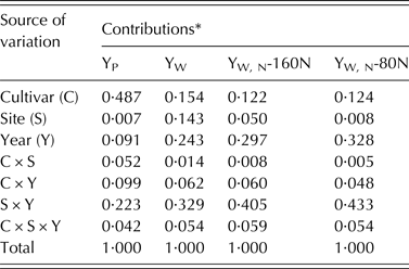
Results from ANOVA showed that cultivars contributed about half of the total variance of YP (Table 7). The cultivar contribution to total variance declined for YW and YW, N. The contribution fraction of year-by-year variance increased from 0·09 for YP to 0·33 for YW, N with 80 kg N/ha. The inverse contribution fractions between YP (optimum managements) and YW, N-80N (low N input) implied that crop management might alter the relative contributions of the sources to yield variations. The interaction between site and year was another important source of yield variation, especially for YW, N-160N and YW, N-80N, contributing >0·40. Under the selected scenarios, site contribution was often low, mainly because the four sites were within the same ecological zone (Fig. 1).
Contribution to total variation of grain yield for seven cultivars across four sites and 30 years and their interactions derived by the analysis of variance (ANOVA)

YP, grain yield potential; YW, water-limited yield; YW, N-160N and YW, N-80N, water- and N-limited yields with N rate 160 and 80 kg/ha, respectively.
* All the variations are significant at the significance level of 0·01. The contribution of the source is calculated as sum of square (SS) of each source divided by total SS.
DISCUSSION
Model evaluations
The CSM–CERES–Maize model in DSSAT v4·6 (Hoogenboom et al. Reference Hoogenboom, Jones, Wilkens, Porter, Boote, Hunt, Singh, Lizaso, White, Uryasev, Ogoshi, Koo, Shelia and Tsuji2015) has been calibrated for >160 cultivars of maize worldwide. However, due to the vast number of cultivars specific to the soils and climates of each region, new local varieties still require calibration. Seven maize cultivars grown in Eastern Canada were calibrated with field experimental data from four sites. The calibrated parameters of the seven cultivars were comparable to the reported values used for maize simulations with the CSM–CERES–Maize model in Canada (Soler et al. Reference Soler, Sentelhas and Hoogenboom2007; Liu et al. Reference Liu, Yang, Drury, Reynolds, Tan, Bai, He, Jin and Hoogenboom2011a , Reference Liu, Yang, Tan, Drury, Reynolds, Zhang, Bai, Jin, He and Hoogenboom b ).
The underestimation during the LAI declining phase could possibly be associated with an over-estimation of LAI in the measured data that were taken with the LAI-2000 at the Stratford site, because the decrease in LAI due to senescent and fallen leaves during the LAI declining phase was only partially detected by LAI-2000 (Stenberg et al. Reference Stenberg, Linder, Smolander and Flower-Ellis1994), while the simulated LAI referred to green LAI excluding the senescent leaves. Therefore, it was more appropriate to compare measured LAI with simulated LAI during the vegetative period rather than the entire growing period. The graphic comparisons showed that LAI was simulated satisfactorily during the LAI increasing phase. Simulation of LAI has frequently been reported as less successful (Ben Nouna et al. Reference Ben Nouna, Katerji and Mastrorilli2000; Lizaso et al. Reference Lizaso, Batchelor, Westgate and Echarte2003b ; Mastrorilli et al. Reference Mastrorilli, Katerji and Nouna2003; Liu et al. Reference Liu, Yang, Drury, Liu and Reynolds2014). Modelling LAI remains difficult due to the complexity of relationships determining substrate allocation and growth and development of leaf area (Ewert Reference Ewert2004). Additional errors might be associated with methodological differences and uncertainties in measuring LAI (Levy & Jarvis Reference Levy and Jarvis1999; Bréda Reference Bréda2003). The less successful simulation of LAI somewhat reduced the simulation precision on yield. However, the simulation precision on yield, with nRMSE < 0·20, was acceptable for the purposes of the present study. Some alternative approaches have been proposed to improve LAI simulation in the CERES–Maize model (Lizaso et al. Reference Lizaso, Batchelor and Westgate2003a ; Nouna et al. Reference Nouna, Katerji and Mastrorilli2003). These alternative approaches need to be further evaluated and integrated into the CSM–CERES–Maize model.
The biomass and yield were well simulated at all sites except Woodslee. A large discrepancy between simulated and measured biomass has been reported for other cultivars, with nRMSE ranging from 0·10 to 0·50 at Woodslee (Liu et al. Reference Liu, Yang, Drury, Liu and Reynolds2014). Similar to the biomass simulation, less successful simulations using the CSM–CERES–Maize model have been reported for maize grain yields at Woodslee (Liu et al. Reference Liu, Yang, Drury, Reynolds, Tan, Bai, He, Jin and Hoogenboom2011a ), with nRMSE as large as 0·39 and EF = −0·70. Simulations for maize grain yield at Woodslee using the crop model STICS were also found to be less successful (Jégo et al. Reference Jégo, Pattey, Bourgeois, Drury and Tremblay2011). Jégo et al. (Reference Jégo, Pattey, Bourgeois, Drury and Tremblay2011) suggested that the underestimation by the model was associated with the fact that precipitation deficit in some periods could be partly compensated for by the capillary rise of groundwater in the experimental fields. The exact reasons for the less accurate simulations at Woodslee should be further explored with more experimental data. Nevertheless, the performance of the CSM–CERES–Maize model was generally acceptable for the purpose of simulating grain maize yield in Eastern Canada, with nRMSE < 0·20, comparable with the results from another study under the same environment but with different cultivars (Soler et al. Reference Soler, Sentelhas and Hoogenboom2007; Liu et al. Reference Liu, Yang, He, Bai, Jin, Drury, Zhu, Yang, Li, Xie, Yang and Hoogenboom2012).
Options to narrow the gaps between actual and potential yields
Maize grain yield is determined by the interactions among genotypic and environmental factors which can be modified by crop management, e.g. choice of cultivar and fertilizer management practices. On the basis of the results from the simulation scenarios, it was clear that the cultivar dominated the variations of YP, and genotypic effects were dramatically reduced under water and N-limited conditions. Cultivars P9411HR and P39D82 produced the highest YP, >18 000 kg/ha under a few favourable year-site environments; this yield was close to the highest record of maize grain yield (19 600 kg/ha) in North America (Nelson & Reetz Reference Nelson and Reetz1986; Tollenaar & Lee Reference Tollenaar and Lee2002). However, the two cultivars did not produce the highest YW at Woodslee, and the highest YW, N-80N at all sites among cultivars. In contrast, the YW, N of a cultivar with low YP such as DKC4627 responded favourably to N rates. The varied responses of maize cultivars to environmental stresses confirmed that cultivars with a high YP usually benefit sites with low environmental stresses (Blum Reference Blum2005), while cultivars with low Yp should be used in regions with high environmental stresses to reduce the risk of yield loss.
An average YP of 15 000 kg/ha for the cultivars with high YP was simulated across the four study sites. This was comparable with 15 800 kg/ha, the highest maize grain yield reported for Ontario (Bruulsema et al. Reference Bruulsema, Tollenaar and Heckman2000). The average YP was slightly lower at Woodslee than at other sites in the simulations. For some other cultivars used in Liu et al. (Reference Liu, Yang, Drury, Liu and Reynolds2014), the simulated YP at Woodslee were higher than at the other three sites (data not shown). As a matter of fact, the simulated YP at Woodslee was also higher than the other three sites for cvar P3573, used in the field experiments at the Woodslee site. These simulation results once more suggested that selecting an appropriate cultivar is the primary option to improve grain yield for a specific environment.
The yield varied among the different soils in a county. In reality, this yield variation among different soils could be small because some soils in a county might not be used for maize production if they were unfavourable to maize and therefore have low benefits for producers; thus, they could be excluded from the statistical data for the county yield YA. The similar values between county- and site yields showed that it was reasonable to use the county yields to represent YA at the present study sites for yield gap analysis.
The simulated YP was about 6000 kg/ha greater than the YA at each site. Two-thirds of this gap between YP and YA was probably associated with water stress, as the average YW was about 11 000 kg/ha for cultivars with high YP. At the experimental sites, the amount of water was on average sufficient for yield potential, as indicated by a total rainfall >550 mm from April to October and a water use efficiency of 30 kg/mm/ha for maize grain (Sadras et al. Reference Sadras, Grassini and Steduto2010). There are years where the total rainfall may be adequate but the timing of the rainfall may be less ideal, when extended periods of drought or excessive precipitation occur. As a result, water stress can contribute to the yield difference between YP and YW in part due to the inter-annual variability and timing of rainfall during the maize growing season. The simulated YW was relatively high and close to YP at St-Jean, where rainfall was more evenly distributed during the crop-growing season than the other three sites. Egli & Hatfield (Reference Egli and Hatfield2014) assessed maize yield gaps in central USA, and they also concluded that large maize yield gaps (>5800 kg/ha) were partially related to the ability of soil water supply in some counties, and irrigation was required to reduce yield gaps in Kentucky and Iowa.
It has been shown before that grain yield of maize as high as 15 800 kg/ha could be realized with trickle irrigation at Chatham in Southern Ontario (Bruulsema et al. Reference Bruulsema, Tollenaar and Heckman2000). The current simulated and observed high yields indicate that it is feasible to improve maize yield by redistributing rainwater to better meet crop demands at locations where a large yield gap exists between YP and YW, such as at Stratford and Woodslee. In Eastern Canada, field crops such as maize are almost never irrigated, as indicated by the fact that irrigated land was reported as <0·10 of cropland (Statistics Canada 2014). The cost of irrigation limits its application primarily to higher-value crops. However, inter-annual grain yield variations of up to 6000 kg/ha under uniform fertilizer N managements have been attributed to rainfall variability in previous, long-term experiments (Liu et al. Reference Liu, Yang, Drury, Reynolds, Tan, Bai, He, Jin and Hoogenboom2011a ). The long-term simulation scenarios showed that two extremely dry years with a grain yield loss of >50% occurred in the 30 years from 1981 to 2010 in Eastern Canada. It is likely that the frequency of such dry years has increased since the 1970s in many regions of the world and will probably continue to increase in the future (IPCC Reference Solomon, Qin and Manning2007). Improving water management may be a potential option for increasing maize yield in Eastern Canada, especially in the face of climate change with even more chances for longer droughts. Although some irrigation technologies have been explored in Eastern Canada in order to improve water use efficiency (Drury et al. Reference Drury, Tan, Gaynor, Oloya and Welacky1996, Reference Drury, Tan, Welacky, Reynolds, Zhang, Oloya, McLaughlin and Gaynor2014; Ibarra et al. Reference Ibarra, Broughton and Bonnell1999; Bernier et al. Reference Bernier, Madramootoo, Mehdi and Gollamudi2010), economic analysis of the irrigation option is still required to ascertain that using irrigation to improve maize grain yields is profitable.
An average yield of 10 000 kg/ha for cultivars with high Yp was simulated for YW, N-160N and this was supported by the observed data. However, a higher grain yield of about 13 000 kg/ha under this N rate simulated for some years was also attained in maize cultivar trials in Eastern Canada (DEKALB 2015). The gap between YW and YW,N illustrated the potential for increasing maize grain yield by improving management of N fertilizer application. In scenario Yw, it was assumed that N supply would synchronize crop demand, so that no N stress would occur. In reality, N application often exceeds the crop demand to maintain sufficient N for all stages in the crop life cycle (Rajsic & Weersink Reference Rajsic and Weersink2008), usually leading to N loss. To achieve synchrony between N supply and crop demand without excess or deficiency is the key to optimizing trade-offs among yield, profit and environmental protection in crop production (Cassman et al. Reference Cassman, Dobermann and Walters2002).
Soil indigenous N supply is generally the primary N source for synchronization of crop demands. The N uptake amount by maize was about 170 kg N/ha with an N harvest index of 0·64 based on a grain yield of 8000 kg/ha for current maize cultivars (Ciampitti & Vyn Reference Ciampitti and Vyn2012). From reported data at a number of sites, mostly in eastern Canada, the soil indigenous N supply in maize field was 76 ± 47·9 kg/ha (Nyiraneza et al. Reference Nyiraneza, Ziadi, Zebarth, Sharifi, Burton, Drury, Bittman and Grant2012), apparently deficient for maize production. Therefore, a fertilizer N rate of 80–160 kg/ha was recommended for growing maize in Ontario by OMAFRA (2014). This recommended rate is generally necessary to balance N input and output. This N fertilizer rate range needs to be verified based on the cultivar and site interaction. The simulated grain yields showed a yield gap of about 3000 kg/ha between the YW and YW, N-80N for the cultivars with high YP, but a much smaller gap for the cultivars with low YP. The different yield gaps among cultivars implied the necessity of varying fertilizer regimes for different types of cultivars, e.g. using high N rates for cultivars with high YP to achieve high yield, rather than trying to increase N rates for cultivars with low YP. Smaller grain yield gaps between the low and high N rates were simulated for Woodslee and Stratford. This is consistent with the previous reports from field experiments in Southern Ontario (Subedi & Ma Reference Subedi and Ma2009). In St-Jean, simulated low YW, N-80N was probably associated with low soil indigenous N supplies determined by N mineralization. The higher organic matter at the Ottawa site and warmer weather conditions at the Stratford and Woodslee sites were favourable for N mineralization (Berendse Reference Berendse1990).
Numerous strategies of fertilizer N for maize have been developed to achieve high yield combined with high N use efficiency (Cassman et al. Reference Cassman, Dobermann and Walters2002). These N strategies include splitting N applications, controlled-release of N fertilizer (Shoji & Kanno Reference Shoji and Kanno1994) and site-specific nutrient management for maize reported from South Asia (Witt et al. Reference Witt, Pasuquin and Dobermann2006). These practices entail higher costs or labour requirements, but certainly increase grain yield based on the reported information. These options need further evaluation by considering the economic and environmental benefits in Eastern Canada.
This study was funded by Agriculture and Agri-Food Canada through the Growing Forward 2 research projects. The authors are indebted to Dr Reinder de Jong for his help in preparing soil data for the experimental sites in Ottawa and St-Jean.