

Competition is not only the basis of protection to the consumer but is the incentive to progress. However, […] destructive competition […] may impoverish the producer and the wage earner.
(Herbert Hoover, States of the Union Address, December 2, 1930)1. Introduction
Although the idea that competitive pressures help reach allocative efficiency to the detriment of investment-inducement has been discussed at length,Footnote 1 we lack a formal framework encompassing the trade-off between static and dynamic efficiency faced by a society choosing whether to deregulate an industry with inelastic demand and its link with political biases. Here, I develop such a model, and I employ it to provide an empirical strategy to structurally estimate the drivers and impact of deregulation, taking as a case study the US power industry.
To elaborate, I build on Laffont and Tirole (Reference Laffont and Tirole1993) and Armstrong and Sappington (Reference Armstrong and Sappington2006), and I compare competition and regulation in a world in which both market institutions and the regulatory contract are selected by a planner who maximizes a weighted average of the consumer surplus and the firms’ utilities, with the weight on the latter rising with society's investment concerns. Before privately learning its marginal and average cost, which can be either high or low with the same ex ante probability, a firm can commit to an unobservable investment increasing the ex post probability of having low cost. Under competition, production is guaranteed by two firms. Each of them serves the entire market at the price proposed by the opponent when able to undercut it, and half of it when the announced prices are the same. Under regulation, on the other hand, production is assured by a monopoly. Hence, the demand on which a firm makes a profit is larger under competition because the prevailing price equals the high cost, which is lower than the price necessary to assure incentive compatibility under regulation. Under competition, however, a firm realizes a profit only when its cost is low and that of the opponent is high, and thus in default of investment, with probability 1:4, which is lower than the odds 1:2 with which a firm makes a profit absent investment under regulation. With inelastic demand, the impact on the expected profit of the larger chance of a rent that regulation entails is bigger than that of the larger demand on which the rent is obtained assured by competition. Hence, the latter entails narrower allocative inefficiencies, but also smaller expected profits, and thus weaker incentives to invest. Society's preferences for competition are thus stronger the less socially relevant cost reduction is. If, instead, investment returns accrue more to the firm's profits than to the consumer surplus, a tension between shareholders and ratepayers arises, and the likelihood that competition is selected rises with the political power of consumers. Finally, since regulation yields a better cost distribution, but competition makes it more likely that the most efficient firms serve the market conditional on such a distribution, competition induces lower expected costs only when investment is not sufficiently effective. Crucially, these implications survive for a generic probability of low cost, a generic number of firms, and a generic correlation between the costs of competing firms, under Cournot competition, for an implicitly motivated regulator, and when society can commit to reimburse investment expenses.
To evaluate the model predictions, I exploit data on the deregulation initiatives implemented in 43 US state electricity markets between 1981 and 1999 and on the operation of the generating plants that served these markets. This choice allows me to focus on institutions similar to those analyzed in the basic model and common to other major regulated markets (Barroso and Maurer, Reference Barroso and Maurer2011). On the one hand, electricity generation lacks the natural monopoly's cost structure that is typical of the distribution and transmission segments, but it serves an inelastic demand (Joskow, Reference Joskow, Griffin and Puller2005). On the other hand, deregulation of the US power industry turned regulated local monopolies into markets offering competitive services at auction-based prices (Joskow, Reference Joskow2009).Footnote 2 To capture society's investment concerns, I posit that a state confronted with costs and/or inefficiencies of input usage larger than those of bordering states should be more willing to stimulate cost reduction (Guerriero, Reference Guerriero2011, Reference Guerriero2013), since even the most pro-consumer community prefers fostering profits and investment to facing the ratepayers’ dissatisfaction. Following Fabrizio et al. (Reference Fabrizio, Rose and Wolfram2007), I focus on fossil fuels because they are the most relevant inputs variable in the medium term.
Consistent with the model, Logit estimates reveal that deregulation was implemented where the marginal fossil fuel cost and the inefficiency of fuel usage was the lowest and politicians were the most pro-consumer. Crucially, these results are not spuriously driven, by the consumers’ willingness to deregulate, to deduct from prices the expenses driven by long-term wholesale contracts and investment in nuclear generation (White, Reference White1996). To elaborate, I control for incentive regulation, share of divested plants, installed capacity, share of generation from nuclear sources, and the residential rate. Moreover, the message of the analysis is the same whether I employ an Ordered Logit distinguishing between the decision to hold a hearing and that of legislating, or I study the timing of deregulation.
Exploiting these results on the drivers of deregulation and the autoregressive structure of the outcome equations, I use the marginal fossil fuel cost lagged three years and the share of bordering states that deregulated as excluded instruments for deregulation to identify its impact on input uses, the inefficiency of fuel usage, and the mark-up of the residential price over marginal costs. Consistent with the limited effectiveness of investment in the industry and conditional on plant and year fixed effects, GMM estimates suggest that deregulation lowered labor and fossil fuel expenses by pushing the most efficient firms to serve the market but it did not reduce the inefficiency of fuel usage. Crucially, the excluded instruments have no direct impact on outcomes and the analysis remains robust to the consideration of the other drivers of deregulation. My results help rationalize the slowdown of the deregulation wave and, in particular, the passage of legislation freezing or repealing reforms in nine out of the 24 states that had deregulated by 2000 (Joskow, Reference Joskow2009).
There are two strands of literature most closely related to the present paper. First, recent literature on “endogenous market design” has also employed the mix of the allocative efficiency versus investment-inducement trade-off and political biases to explain the distribution of other key competitive pressures.Footnote 3 Building on similar foundations, I provide instead the first normative and positive analyses of the choice of whether to regulate firms or to allow them to compete in the presence of investment inefficiencies and inelastic demand. Second, a long stream of empirical research has tried to address the endogeneity of deregulation by either controlling for plant and time-fixed effects (Cicala, Reference Cicala2015; Craig and Savage, Reference Craig and Savage2013; Fabrizio et al., Reference Fabrizio, Rose and Wolfram2007; Parker et al., Reference Parker, Kirkpatrick and Zhang2008) or using political preferences as excluded instruments (Gugler et al., Reference Gugler, Rammerstorfer and Schmitt2013; Zhang, Reference Zhang2007). These identification strategies display two major problems. First, the fixed effects OLS estimator might grossly underestimate the cost reduction brought by deregulation because this reform is more likely in states that are less investment-concerned, and thus exert a systematically small effort to optimize input uses and reduce the inefficiency of fuel usage. By relying on time-varying excluded instruments, I can tackle this issue. Second, political preferences might directly shape input uses (Besley and Coate, Reference Besley and Coate2003) and employing them as excluded instruments would fail to expunge the endogenous component of deregulation. By using the lagged marginal fossil fuel cost and the deregulation of bordering states, I do not incur this simultaneity problem.
The paper proceeds as follows. First, I describe in section 2 the key facts about the deregulation of the US electricity industry to inform my general model of market design, which I illustrate in section 3. Next, I state the key model predictions in section 4, and I discuss my test in section 5. Finally, I conclude in section 6, and I report the tables (proofs, sample construction, data sources, and supplementary results) in the (online) appendix.Footnote 4
2. Deregulating the US electricity industry
Starting from the 1907 shift from municipal to state regulation, the US electricity industry was dominated by vertically integrated investor-owned utilities – IOUs hereafter – operated as regulated monopolists over the generation, transmission, and distribution of electricity within their localized geographic market (Knittel, Reference Knittel2006). Prices were determined by Public Utility Commissions – PUCs hereafter – at the firm level to assure a specific rate of return on investment after recouping accounting costs of service, i.e. cost-of-service regulation (Joskow, Reference Joskow1974). After decades of productivity growth and falling electricity prices, serious problems emerged during the 1970s as fossil fuel prices, inflation, and interest rates rose (Joskow, Reference Joskow1974). On the one hand, PURPAFootnote 5 pushed the less efficient IOUs to sign with the more cost-effective ones long-term wholesale contracts for energy (Joskow, Reference Joskow1989), which became a burden in the 1980s because of the continuously rising fossil fuel prices. On the other hand, the interest rate payments related to the investments in alternative – particularly nuclear – generation technologies skyrocketed (Joskow, Reference Joskow, Griffin and Puller2005). These two instances brought about both high electricity prices and a growing gap between the regulated rates and the value of generation in the regional wholesale markets, pushing the powerful industrial users to lobby for stronger competitive pressures (White, Reference White1996).Footnote 6
In the attempt to enhance efficiency, many PUCs replaced, over the 1980s and the early 1990s, cost-of-service regulation with higher-powered regulatory incentive schemes, but with limited effects (Guerriero, Reference Guerriero2013). Accordingly, the 1992 Energy Policy Act required consideration of opening up the wholesale markets to competition. Deregulation initiatives were launched by the state legislatures but discussed and ratified during quasi-judicial hearings (Joskow, Reference Joskow, Griffin and Puller2005). Open to both IOUs and consumers, these proceedings were directed by the PUC commissioners, who first examined experts and received evidence, and then specified “findings of fact” upon which the regulatory order was based (Joskow, Reference Joskow1974). To capture these features, I assume that the market institutions and the regulatory contract are selected by a planner who maximizes a weighted average of the firms’ utilities and the consumer surplus. There is, moreover, a broad agreement that the goal of the deregulation hearings was to obtain a market design assuring “adequate, safe, reliable, and efficient energy services at fair and reasonable prices” (EIA, 2003: 24). Hence I maintain that the weight on the firms’ utilities rises with society's investment concerns and, when investment returns accrue more to the firm's profit than to the consumer surplus, with the political power of shareholders. This assumption captures the idea that, although the widest consensus is needed to approve reforms, politicians pander to their constituency (Joskow, Reference Joskow, Griffin and Puller2005).
By 1998, every jurisdiction had launched deregulation hearings, and by 2000, almost half had approved legislation introducing some form of competitive retail access (Fabrizio et al., Reference Fabrizio, Rose and Wolfram2007). As a result, in deregulated states, IOUs own a limited fraction of generation capacity, and plants sell electricity through either auction-based spot markets or long-term contracts calibrated on the expected bids (Barroso and Maurer, Reference Barroso and Maurer2011: 65–73). “The promise was that these reforms would lead to lower costs and lower average retail price levels […] compared to regulated monopoly alternative, while maintaining or enhancing system reliability” (Joskow Reference Joskow, Griffin and Puller2005: 37). The reality, instead, has been one of “insufficient net revenues to support the capital costs of an efficient portfolio of generating facilities” (Joskow Reference Joskow2006: 2), and most of the generating capacity that has recently entered service was built by "municipal utilities that have not been subject to [deregulation]” (Joskow Reference Joskow2008: 28). Hence, it is not surprising that almost half of the states that had deregulated by 2000 reacted to projections of shortages by local system operators and electric power supply emergencies by repealing existing legislation (Joskow, Reference Joskow2009).
3. Endogenous market design
To clarify the mix of the static versus dynamic efficiency trade-off and political biases, I first study the former by envisioning a benevolent planner and, then, I drop this assumption.
A benevolent planner
Preferences
The representative consumer demand is q(p) > 0 for $p\in \lsqb {0,\bar{p}} \rpar$ and 0 for $p \ge \bar{p}$
 , and q ′(p) < 0. Production is assured by either one monopoly under regulation or two firms under competition. While q(p), p, and the cost distribution are common knowledge, the marginal and average cost c i is observed only by the firm and equals either c L or c H > 0 with odds 1/2. Let Δ ≡ c H − c L > 0. Under institution j ∈ {R, C}, a type i ∈ {L, H} firm maximizes the rent $U_i^j$
 , which equals the profits π(p i, c i) ≡ q(p i)(p i − c i) plus a type-dependent governmental transfer t i ≥ 0 under regulation. The social welfare W j equals the sum of the consumer surplus $S\lpar p \rpar = \mathop \smallint \limits_p^{\bar{p}} q\lpar x \rpar dx$
 and each firm's rent evaluated at α ∈ [0, 1) minus the transfer evaluated at the shadow cost of public funds 1 + λ > 1 – i.e. $W^R = S\lpar p \rpar + \alpha U_i^R -\lpar {1 + \lambda} \rpar t_i$
 and $W^C = S\lpar p \rpar + \alpha \lpar {U_{i,1}^C + U_{i,2}^C} \rpar$
 , where I have emphasized the existence of two firms under competition. While λ originates, for instance, from distortionary taxation α is strictly lower than 1 because of the focus of regulation on consumer welfare (Joskow, Reference Joskow1974).Footnote 7 I also assume that the expected social welfare is strictly concave and the demand is, as in the relevant empirical cases, inelastic:Footnote 8
Assumption 1:
The demand function satisfies ${q}^{\prime \prime}\lpar p \rpar \lpar {\bar{p}-c_L} \rpar + {q}^{\prime}\lpar p \rpar \lt 0$ and $\; \varepsilon _{p,q} = -\; \displaystyle{{{q}^{\prime}\lpar p \rpar p} \over q} \lt 1$
 .
The timing
Market design and production proceed according to the following timeline:
-
t = 1: The planner selects institution j on the basis of the sum of the expected social welfare and a mean zero pro-regulation shock δ distributed on [ − ∞, ∞] with density f and CDF F. Under regulation, a regulator acting as a perfect agent of the planner offers the monopoly a menu of (t i, p i) pairs conditional on the firm's report on c i but not on investment.
-
t = 2: Under market design j, each firm commits to an unobservable investment I j costing ψ(I j) > 0 with ψ ′ > 0, ψ ′′ >0, ψ(0) = 0 and lim I→1 2ψ ′(I j) ≥ S(c L) − S(c H). I j raises the odds of c L to (1 + I j)/2. The firms’ choices under competition are contemporaneous.
-
t = 3: Each firm discovers its piece of private information, which is c i.
-
t = 4: Under regulation, the firm makes its report and the corresponding contract is executed. Under competition, the two firms bid a price, and the one offering the lowest price serves the entire market at the opponent's bid. In case of a tie, the market is evenly split.
Discussion
To evaluate the generality of the setup, several remarks should be borne in mind. First, considering the ex ante case in which the market is designed before each firm discovers its type is justified by the sizable uncertainty over the cost structure typical of regulated markets (Auriol and Laffont, Reference Auriol and Laffont1992; Laffont and Tirole, Reference Laffont and Tirole1993). Second, focusing on a monopoly instead of a duopoly and assuming that the monopolist pre-exists to the market design are consistent with the empirically relevant case of deregulation.Footnote 9 Third, since cost reduction is financed through the expected rent, α is a measure of society's dynamic efficiency concerns (Guerriero, Reference Guerriero2011, Reference Guerriero2013). Fourth, δ captures determinants of market design unrelated to technology and political biases, like generalized trust (Aghion et al., Reference Aghion, Algan, Cahuc and Shleifer2010). Fifth, I treat investment as non-monetary – e.g. the effort in managing a plant more efficiently – but the model extends to monetary investments (see the online appendix). Finally, the gist of the model will be unaffected should the ex ante correlation between types be positive (see note 10), the probability of low cost be generic (see note 11), the regulator be career-concerned, society be able to commit to reimburse investment costs, and the number of competing firms be generic and under Cournot competition (see the online appendix).
Regulation versus competition: static efficiency
Regulation
As Laffont and Tirole (Reference Laffont and Tirole1993) and Vives (Reference Vives2008), I focus on symmetric pure strategy equilibria. Starting with regulation, the planner dislikes leaving a rent to the firm and prefers to let both types produce. Hence, the regulator offers type-dependent price-transfer pairs such that the firm truthfully reports a c i = c L – i.e. q(p L)(p L − c L) + t L = q(p H)(p H − c L) + t H – and operates if c i = c H, i.e.$\; U_H^R = 0$ . Hence, ac L-type enjoys an informational rent $U_L^R = \Delta q\lpar {p_H} \rpar$
 (Myerson, Reference Myerson1979), and the expected social welfare equals:

where w i(p i, c i) = S(p i) + (1 + λ)π i(p i, c i) and I made explicit that the regulator anticipates $\hat{I}^R$ . To limit the c L-type's rent, the regulator reduces the c H-type's allocation compared to the full information optimum obtaining the expected social welfare he would get was the firm's cost observable but its higher realization equal $\hat{c}_H\equiv c_H + \textstyle{{1 + {\hat{I}}^R} \over {1-{\hat{I}}^R}} \big( {\textstyle 1-{\alpha \over {1 + \lambda}}} \big)\Delta$
 . No distortion is needed if the report is c L, since there is no incentive to under-report. Thus, the price maximizes w L( · ) for cost c L and w H( · ) for cost $\hat{c}_H$
 . Hence, p L = c L and p H equals $\hat{c}_H$
 , which tends to the monopoly price if λ is large, and thus transfers entail large social costs. The expected social welfare under regulation can, then, be rewritten as:

In the following, I assume that $\bar{p} \gt \hat{c}_H$ for concreteness and λ = 0 for simplicity. This last restriction can be easily eliminated as illustrated in the online appendix.
Competition
Because of the Vickrey auction-type structure of competition, truth-telling is the only symmetric pure strategy equilibrium since a c H-type strictly prefers to bid c H, whereas playing c L is a c L-type's best response to an opponent with high cost and exhausts its incentives to undercut an opponent with low cost. To see why this is the case, notice that the expected profit of a c L-type playing p L <c H equals $\textstyle{{1 + {\hat{I}}^C} \over 4}q\lpar {p_L} \rpar \lpar {p_L-c_L} \rpar + \textstyle{{1-{\hat{I}}^C} \over 2}q\lpar {c_H} \rpar \Delta$ . Overall, the equilibrium price equals c H except when both firms have low cost, and a firm enjoys a profit only when its type is c L and the opponent's one is c H. This happens with probability$\; \lpar {1/4} \rpar \lsqb {1-{\lpar {{\hat{I}}^C} \rpar }^{2}} \rsqb$
 .
The expected social welfare under competition is then:

Regulation versus competition: dynamic efficiency
$\hat{I}^R$ maximizes the expected firm's rent $E\lpar {U_i^R} \rpar$
 minus investment costs ψ(I R), i.e.:

where the dependence of $\hat{c}_H\equiv c_H + \displaystyle{{1 + {\hat{I}}^R} \over {1-{\hat{I}}^R}}\lpar {1-\alpha} \rpar \Delta$ on $\hat{I}^R$
 and not I R incorporates the lack of regulatory commitment (see Laffont and Tirole, Reference Laffont and Tirole1993: 101). Similarly:

There are two key observations. First, $0 \lt \hat{I}^j \lt \hat{I}^{j,*} \lt 1$ , where each socially optimal $\hat{I}^{j,*}$
 maximizes the expected social welfare less investment costs under full information and regime j. Second, the extent of underinvestment is wider under competition. To elaborate, a competitive firm obtains a positive mark-up on a larger demand – i.e.$\; q\lpar {c_H} \rpar \gt q\lpar {{\hat{c}}_H\lpar {{\hat{I}}^R} \rpar } \rpar \;$
 – but less often – in half of the cases in which $\hat{I}^R = \hat{I}^C = 0$
 – than a regulated one.Footnote 10 Yet the larger probability of getting a rent, which is akin to a change in price, more than compensates the fall in demand because of assumption A1. As a consequence, $\hat{I}^R \gt \hat{I}^C$
 . This gap is widened by the mix of the ex post correlation between costs and the strategic complementarity of pricing decisions under competition (see also Vives, Reference Vives2008).
The static versus dynamic efficiency trade-off
In t = 1, competition is chosen when W C >W R + δ that, for δ = 0, can be rewritten as


Under regulation, a rise in α has a triple impact on WR. First, it increases the ex post probability of c L by raising $\hat{I}^R$ . This positive impact on WR is the “investment-enhancing” effect of a rise in α on market design. Second, as α rises, allocative inefficiencies fall – i.e. $\hat{c}_H$
 goes down – because of the larger social value of the firm's rent. This positive impact on W R is the “distortion-curbing” effect of a rise in α on market design. Third, allocative inefficiencies become more necessary due to the more favorable cost distribution. This negative impact on W R is the “distortion-enhancing” effect of a rise in α on market design. Under competition, however, a rise in α entails a greater social value of the firm's profit but does not affect investment, which unlike regulation is picked to maximize a function of its private – and not social – returns. This positive impact on W C is the “profit-value” effect of a rise in α on market design. While the investment-enhancing effect is larger than the distortion-enhancing one because of the inelastic demand, the distortion-curbing effect is larger than the profit-value one if investment is sufficiently effective. Overall, a rise in α makes regulation more socially valuable under the following sufficient condition, which can be relaxed at the cost of more cumbersome algebra:Footnote 11
Assumption 2:
ψ ′(1/2) ≤ (Δ/8)q(c H).
Market design becomes, then, an indirect instrument to solve dynamic inefficiencies and:Footnote 12
Proposition 1:
Under assumptions A1 and A2, the probability that competition is chosen – i.e. F(W C − W R) – falls with society's investment concerns α.
This belongs to those findings suggesting that institutions curbing rent-extraction can be optimal when investment inducement is socially relevant (Guerriero, Reference Guerriero2011, Reference Guerriero2013; Sappington, Reference Sappington1986). This implication also applies to communities less culturally inclined to accept that some citizens gain from investment, provided that the local technology is sufficiently less efficient than those of adjacent jurisdictions. Indeed, even the most pro-consumer community prefers fostering profits and investment to facing ratepayers’ dissatisfaction.
Relationship with the evolution of the US electricity industry
Proposition 1 is consistent not only with the estimates illustrated in section 5 but also with the evidence on other competitive pressures experimented in the US electricity industry. First, the beginning of the 1900s reforms from a municipal regulation with its hold-up problems to a fair rate of return state regulation were implemented first where capacity shortages were most severe (Knittel, Reference Knittel2006). Second, Guerriero (Reference Guerriero2011) documents that, between 1960 and 1997, appointment, which curbs the regulators’ incentives to discover the firm's cost raising its rent, was embraced by the states characterized by the largest generation costs. Finally, Guerriero (Reference Guerriero2013) shows that, between 1981 and 1999, more powerful incentive contracts, limiting allocative inefficiency and rent extraction, were signed by IOUs operating in states where marginal costs and prices were higher than those of neighboring ones.
The political economy of market design
A tension between shareholders and ratepayers arises when investment returns accrue more to the firm's rent than to the consumer surplus, e.g. marketing. Then, market design can be distorted by political biases. To clarify the point in the sharpest way, I consider an investment possibly implemented after t = 4, costing $\bar{I} \gt 0$ , raising the firm's ex post rent – but not the consumer surplus – of $\bar{\beta} \bar{I}$
 with probability μ and zero otherwise, and affected by an aid fixed by a political party possibly different from the planner.
Setup
To elaborate, the timing is augmented with two periods:
-
t = 5: The planner$\; \tilde{m}$
 , who is either the pro-shareholder party s or the pro-consumer party r and has selected institution j in t = 1, faces an election with exogenous winning probability$\; x_{\tilde{m}}$. Next, the winner of the election m ∈ {s, r} implements an aid equal to ρ m > 0 times the firm's rent and paid out to the firm after the investment is undertaken.
-
t = 6: The firm possibly commits to the investment.


The firm has no wealth to post as a bond in the case of unsuccessful investment except the ex post rent, which is now $\lpar {1 + \rho_m} \rpar \hat{U}_i^R$ . The ex post rent, however, is initially illiquid and can only be pledged as collateral against borrowing $\bar{I}$
 . The debt contract is such that the lender receives a payment$\; \tau \bar{I}$
 in the case of a successful project and a collateral$\; \underline{\beta} \bar{I} \gt 0$
 , with $\bar{\beta} \gt \tau \gt \underline{\beta}$
 , otherwise (Besley and Ghatak, Reference Besley, Ghatak, Rosenzweig and Rodrik2010). Thus, only thec L-type invests if the limited liability constraint $\lpar {1 + \rho_m} \rpar \hat{U}_i^R -\underline{\beta} \bar{I} \ge 0$
 is satisfied and if the lender agrees – i.e. $\mu \lpar {\bar{\beta} -\tau} \rpar \bar{I}-\lpar {1-\mu} \rpar \underline{\beta} \bar{I} \ge 0$
 and $\mu \tau \bar{I} + \lpar {1-\mu} \rpar \underline{\beta} \bar{I} \ge \bar{I}$
 , which are both true if $\bar{\beta} \ge \mu ^{-1}$
 . As a result, in t = 1 the planner evaluates the investment aid $\rho _m\hat{U}_i^R$
 at 1 + λ and the limited liability constraint at $1 + \chi _{\tilde{m}}$
 , where $\chi _{\tilde{m}}$
 captures his willingness to boost ex post investment. Finally, to ease the exposition, I assume that λ > 0, that the firm chooses $\hat{I}^R$
 without considering ex post investment,Footnote 13 and that the parameters are in the following relationships:
Assumption 3:
ρ s > ρ r; χ s > λ > χ r; $\bar{\beta} \mu \ge 1$ .
Discussion
A handful of observations help stress the solidity of this simple setup. First, the aid technology incorporates into the setup the huge transfers from the federal and state governments to IOUs, financed through distortionary taxes (Metcalf, Reference Metcalf2008).Footnote 14 Second, at the cost of more cumbersome algebra, my results will be similar should investment decisions be continuous. Third, the assumption that the winning party cannot reform the market institution captures the commitment period typical of regulation (Guerriero, Reference Guerriero2013). Fourth, the exogeneity of $x_{\tilde{m}}$ matches the idea that regulation is bundled at election with more salient policies (Besley and Coate, Reference Besley and Coate2003). Finally, the hypothesis that the pro-shareholder party is more willing to subsidize investment expenses is consistent with politicians’ strategic incentives to adopt extremist platforms in order to empower their supporters (Guerriero, Reference Guerriero2011).
Equilibrium
For δ = 0 and $\tilde{x}\equiv \rho _rx_r + \rho _sx_s$ , a $\tilde{m}$
 planner picks competition if:

The expected firm's rent is again smaller under competition, and the following pattern arises:
Proposition 2:
Under assumptions A1, A2, and A3, the odds that competition is selected fall with the planner's hold on power $\; x_{\tilde{m}}$ and are smaller if he is pro-shareholder.
This result originates from the mix of the asymmetry in the parties’ preferences and the uncertainty of elections, and is similar to the strategic dynamics proposed by a lively political economy tradition (Hanssen, Reference Hanssen2004). To illustrate, a higher probability of being reelected and then fixing a larger (smaller) aid, without facing a new market reform, pushes a pro-shareholder (consumer) planner to value regulation more because of the even larger rent accruing to his constituency (prospect of underinvestment). This incentive can drive inefficient reforms and, for instance, a pro-consumer party to prefer competition despite the prospect of sizable dynamic inefficiencies. Crucially, the normative conclusions summarized in propositions 1 can be also derived from the positive analysis synthesized in inequality (4).
Relationship with the evolution of the US electricity industry
Proposition 2 not only matches the evidence discussed in section 5 but, also, that on other competitive pressures experimented in the US electricity industry. First, state regulation was favored by stronger residential consumer interests, i.e. lower penetration rates among residential users (Knittel, Reference Knittel2006). Second, Guerriero (Reference Guerriero2011) shows that PUC commissioners are elected when consumers are more politically powerful. Finally, Guerriero (Reference Guerriero2013) documents that, under the very same circumstances, less powerful incentive rules are selected.
4. Testable predictions
The mix of the static versus dynamic efficiency trade-off and political biases implies, then, the following testable prediction on the determinants of market design:
Prediction 1:
The likelihood of deregulation decreases with society's dynamic efficiency concerns and with the incumbent's hold on power, and it is smaller when he is pro-shareholder.
Since regulation yields a better cost distribution but, conditional on types, competition leads the most efficient firms to serve the market, deregulation lowers expected costs if:

which must be the case for $\displaystyle{{1-2\lpar {{\hat{I}}^R-{\hat{I}}^C} \rpar -{\lpar {{\hat{I}}^C} \rpar }^2} \over 4}\lpar {c_L-c_H} \rpar \lt 0\leftrightarrow \hat{I}^R \lt \lpar {1/2} \rpar \lsqb {1 + 2{\hat{I}}^C-{\lpar {{\hat{I}}^C} \rpar }^2} \rsqb$ . This inequality holds true if ψ ′ is not too small and α not too large, i.e. investment is not sufficiently effective because of sizable marginal investment costs and society's limited investment concerns. Both features represent two key characteristics of the US electricity industry as suggested by its suboptimal technological speed (Margolis and Kammen, Reference Margolis and Kammen1999) and a regulatory focus on keeping prices from increasing (Joskow, Reference Joskow1974). Building on this remark, the second testable prediction deals with the link between market design and outcomes:
Prediction 2:
Compared with regulation, competition limits allocative inefficiencies given the initial cost distribution, without, however, improving such distribution over time.
Next, I test both predictions in turn, employing US electricity industry data.
5. Evidence
To control for the other post-1980 competitive pressures, I focus on the 1981–1999 period. In addition, I exclude the District of Columbia and seven states since, for these jurisdictions, I do not always observe political biases and/or outcomes. Hence, I study the drivers of deregulation by using a balanced panel of 43 states s spanning each year t between 1981 and 1999, whereas I assess the impact of the market design by analyzing an unbalanced panel of 503 plant-epochs p observed in the aforementioned 43 states between 1981 and 1999 for a total of 8,059 yearly data points. Plant-epochs are obtained by assigning a new identifier to each combined-cycle gas and steam turbine power plant surveyed by FERC in the 43 states when its capacity changed more than 40 MW or 15% (Fabrizio et al., Reference Fabrizio, Rose and Wolfram2007).
Endogenous deregulation
Testing prediction 1 requires to both measuring deregulation and its determinants and selecting an appropriate model of the probability of deregulation.
Measuring deregulation
As suggested by Fabrizio et al. (Reference Fabrizio, Rose and Wolfram2007), IOUs acted before legislation altering their behaviors soon after the deregulation hearings. Therefore, I capture the shift from a regulated to a competitive market design with the dummy Deregulation, which equals one for states or IOU plants in states that deregulated, beginning in the year of the first deregulation hearing. To evaluate the possibility that utilities did not respond until legislation, I perform the following two robustness checks. First, I substitute Deregulation with the dummy Law, which turns on in the year the state passed legislation. Second, I consider the indicator Deregulation-O, which equals 3 beginning in the year of legislation, 2 beginning in the year of the first deregulation hearing, and 1 otherwise. The results of both checks are consistent with the testable predictions (see the online appendix).
Measuring the determinants of deregulation
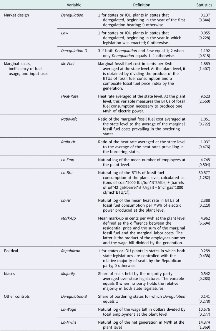
To capture society's investment concerns, I assume that a state confronted with marginal costs and/or inefficiencies of input usage that are larger than those of bordering states should be more willing to stimulate cost reduction to catch up (see Guerriero, Reference Guerriero2011, Reference Guerriero2013), and I focus on fossil fuels because they are the key inputs variable in the short and medium run covered by my sample (Fabrizio et al., Reference Fabrizio, Rose and Wolfram2007). To alleviate the possible issues of the endogeneity of these proxies moreover, I consider them to have lagged three years. The rationale of this choice is as follows. First, market design at time t is a function of the ex ante cost distribution, which is extracted during deregulation hearings from the costs observed in t−1 (Joskow, Reference Joskow2009). Second, I document that the outcome equations display an AR(1) structure (see below). Together these two remarks imply that instruments related to input uses and costs are exogenous only if lagged three years or more. I consider (1) the arithmetic mean – i.e. average thereafter – of the marginal fossil fuel cost in cents per Kwh, i.e. Mc-Fuel; (2) the average of British thermal units (BTUs) of fossil fuels necessary to produce one MWh – i.e. Heat-Rate,Footnote 15 which captures inefficiencies of fuel usage; (3) the ratio of the average marginal fossil fuel cost to the average of the marginal fossil fuel costs in the bordering states, i.e. Ratio-Mfc; (4) the ratio of the average heat rate to the average of the heat rates in the bordering states, i.e. Ratio-Hr. Mc-Fuel and Heat-Rate allow the comparison of a state with the rest of the Union, whereas the other two proxies take as a reference group the bordering states (see Table 1 for a summary of all variables). The gist of my analysis will survive, should I substitute the arithmetic mean of either the marginal fossil fuel cost or the heat rate in the bordering states with their average weighted by population size (see the online appendix).
Summary of variables

Notes: BTU, British thermal units. See the online appendix for a description of the sources of each variable. The last column reports the mean value and, in parentheses, the standard deviation of each variable. Both are computed building on the sample used in Table 2 except for Ln-Emp, Ln-Btu, Ln-Hr, Mark-Up, Ln-Wage, and Ln-Mwhs, which are calculated employing the sample used in Table 3.
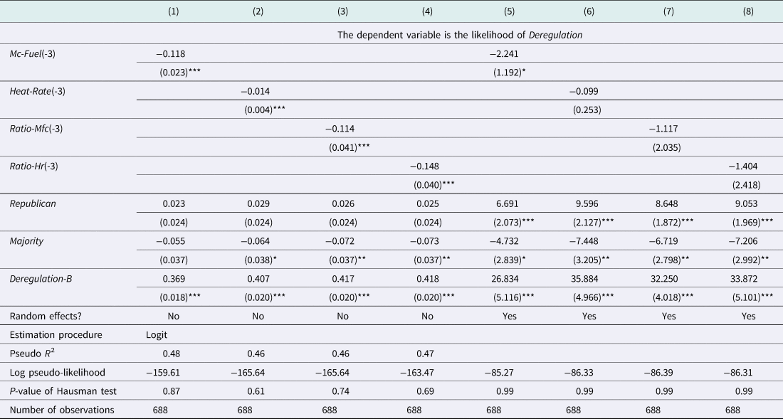
Endogenous market design

Notes
1. The unit of observation is state per year.
2. The entries are marginal effects.
3. In parentheses are reported the standard errors, which are robust in columns (1)–(4).
4. *** denotes significant at the 1% confidence level; **, 5%; *, 10%.
5. While the FE Logit estimator is consistent but inefficient under both the null and the alternative hypotheses, the Logit and RE Logit estimators are consistent and efficient under the null hypothesis but inconsistent under the alternative one. Hence, rejecting the null hypothesis of the Hausman test in columns (1)–(4) (in columns (5)–(8), i.e. the unobserved state fixed effects are uncorrelated with the other covariates) implies that the FE Logit estimator should be preferred to the Logit (RE Logit) one.
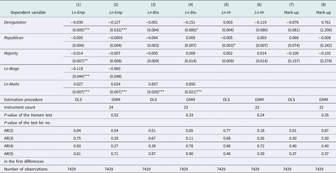
Endogenous market design and outcomes — OLS versus GMM

Notes
1. The unit of observation is plant-epoch per year.
2. In parentheses are reported the robust standard errors, which are also corrected following Windmeijer (Reference Windmeijer2005) in columns (2), (4), (6), and (8) where a two-step difference GMM procedure is employed.
3. *** denotes significant at the 1% confidence level; **, 5%; *, 10%.
4. All specifications consider also Scrubber and plant and year fixed effects.
5. In columns (2), (4), (6), and (8), the endogenous variable is Deregulation, and the excluded instruments are Deregulation-B and Mc-Fuel(-3). Moment conditions are collapsed to have only one instrument column per year.
6. The null hypothesis of the Hansen test of over-identifying restrictions is that the instruments, as a group, are exogenous.
7. The Arellano–Bond test for serial correlation is applied to the differenced residuals. A test rejecting the null hypothesis of no serial correlation of order l in the differenced residuals detects serial correlation of order l-1 in levels.
Turning to political biases, a large body of literature claims that Republicans have been more attentive to the shareholders’ interests (Teske, Reference Teske2004). Yet it is also true that there are more shareholders of firms buying electricity than there are of firms selling it, and thus Republican politicians might be more interested in safeguarding the industrial consumers’ welfare than in maximizing the firms’ profits. Hence, I consider a dummy that turns on if both state legislatures were under the Republicans’ control, i.e. Republican. Regarding the incumbent's hold on power, I follow Hanssen (Reference Hanssen2004), and I consider a variable equal to the share of seats held by the majority party averaged over state legislatures and to 0 when no party holds the relative majority in both state legislatures, i.e. Majority. If regulation is not salient at elections (Besley and Coate, Reference Besley and Coate2003), both Republican and Majority are exogenous. Finally, the diffusion of a new institution displays distinctive imitation patterns whereby a reform in one jurisdiction should shift support in the neighboring jurisdictions, without affecting performance before implementation (Teske, Reference Teske2004). To capture this exogenous process, which produces a second exclusion restriction in testing prediction 2, I consider the share of bordering states that deregulated, i.e. Deregulation-B. My results will be similar should I switch to Deregulation either averaged over bordering states and weighted by their population size or averaged over all other states (see the online appendix).
Model selection
By linearizing inequality (4) and decomposing the shock δ in an idiosyncratic component δ s,t less a state-specific term c s, endogenous market design is described by:

where c s captures unobserved time-invariant drivers of market design, Xs,t incorporates the proxies for the strength of society's investment concerns and the political biases, Zs,t gathers Deregulation-B and possibly the extra controls discussed below, and F is assumed Logistic. I estimate equation (6) by either a Logit model, which forces the c s to be equal across s, or a random effects – RE – Logit model,Footnote 16 which requires that $c_s\vert {\; {\bi W}_s \sim N\lpar {0,\sigma_c^2} \rpar }$ , where Ws is the union of Xs,t and Zs,t. This strategy is supported by the following two pieces of evidence. First, I never reject the null hypothesis of the Hausman test of the RE versus the fixed effects – FE – Logit model – i.e. unobserved state effects are uncorrelated with the regressors at a level anywhere lower than 0.99 (see Table 2). Second, I never reject the null hypothesis of the Hausman test that the Logit – and not the FE Logit – model is appropriate at a level anywhere lower than 0.61 (see Table 2). These patterns are driven by the loss of 336 observations in the computation of the conditional FE Logit model likelihood.
Main results
While columns (1)–(4) of Table 2 report the estimates of the Logit model, columns (5)–(8) list those of the RE Logit model. For ease of interpretation, I focus on the Logit model marginal effects, which give the percentage change in the likelihood of Deregulation when a control rises by one percentage point, and the RE Logit model coefficients. Both are consistent with prediction 1, and the implied effects are large. Starting with the impact of society's dynamic efficiency concerns, the likelihood of deregulation falls by: (1) 16.6 percentage-points as a result of a one-standard-deviation rise in Mc-Fuel(-3); (2) 3.6 percentage-points as a consequence of a one-standard-deviation increase in the lagged average heat rate; (3) 8.2 percentage-points as Ratio-Mfc(-3) increases by one-standard-deviation; and (4) 7 percentage-points as Ratio-Hr(-3) rises by one-standard-deviation. These coefficients are significant at 1%. The estimates of the RE Logit model deliver a similar message, although the coefficients are less significant. More mixed is the evidence on the role of political biases. The planner's hold on power tends to decrease the likelihood of deregulation as expected, whereas the sign of the coefficient on Republican is consistent with Prediction 1 only if one is inclined to think that industrial consumers were politically stronger than IOUs (Joskow, Reference Joskow, Griffin and Puller2005). Finally, deregulation was driven by the decisions of bordering states.
Robustness checks
The online appendix gathers the following battery of robustness checks.
First, the gist of the analysis stands when I include in Zs,t either stepwise or all together, year dummies controlling for countrywide shocks and changes in federal policies and the five drivers of deregulation most discussed by the extant literature.Footnote 17 The first one is a dummy for whether a state adopted incentive regulation, i.e. PBR. These reforms have granted a larger rent to the firm inducing less stringent society's dynamic efficiency concerns (Guerriero, Reference Guerriero2013). The other four controls capture the idea that deregulation was implemented where regulated prices were high and most exceeded the value of electricity in the wholesale markets (White, Reference White1996). They are: (1) the share of plants divested because of deregulation; (2) capacity in MW; (3) the share of generation from nuclear sources; (4) the residential price in cents per Kwh.
Second, the message of the empirical exercise is consistent with Prediction 1 if I analyze the ordered competitive pressure indicator Deregulation-O via the Ordered Logit estimator.
Third, I document that the results of my analysis are qualitatively similar when I study, instead, the timing of deregulation by running Exponential Survival models.
Finally, I show that the analysis is quite similar when the errors, instead of being robust to generic heteroskedasticity and serial correlation, allow for clustering by state.
Implications
Ultimately, Table 2 suggests that regulation was retained where the need to accommodate investment concerns was sufficiently pressing and the consumers’ political power weak enough. This interpretation aligns with both anecdotal and empirical evidence on the underinvestment in the industry between the oil crises of the 1970s and the deregulation phase (Joskow, Reference Joskow1974; Margolis and Kammen, Reference Margolis and Kammen1999), and it implies that the distribution of the design of the electricity market across US states is not random. Therefore, estimates produced by OLS regressions of outcomes on deregulation will be inconsistent, and the key challenge of the following tests of Prediction 2 is to properly address endogeneity issues.
Endogenous market design and outcomes
Testing Prediction 2 requires measuring the efficiency of a single-output plant and its drivers and selecting an appropriate model of the effect of deregulation on such an outcome.
Measurement and model selection
I embrace a two-step strategy. First, I follow Fabrizio et al. (Reference Fabrizio, Rose and Wolfram2007), and I evaluate whether deregulation pushed the plants to use the best mix of variable inputs in the short and medium run given their prices. Second, I follow Craig and Savage (Reference Craig and Savage2013), and I test whether the usage of fossil fuels became more efficient and, more generally, whether investment incentives – as captured by the mark-up of price over marginal costs – increased after deregulation.
Starting from my first test, I assume, for concreteness and to compare my results with the extant empirical literature (Fabrizio et al., Reference Fabrizio, Rose and Wolfram2007), that the constant returns to scale production function considered in the model is indeed a Cobb–Douglas function of the technological parameter A p,j,t, labor L p,j,t and fossil fuel F p,j,t, i.e. $A_{p,j,t}L_{p,j,t}^\gamma F_{p,j,t}^\eta \;$ with γ + η = 1. This hypothesis also reflects the fact that while fuel inputs are varied in response to real-time dispatching and operational changes and staffing can be adjusted over the medium run, capital is chosen at the time of the plant's construction, and should then be considered as fixed (Fabrizio et al., Reference Fabrizio, Rose and Wolfram2007). Therefore, p will minimize, in t and under regime j, the total costs W p,j,tL p,j,t + S p,j,tF p,j,t, given wages W p,j,t and fossil fuel prices S p,j,t, and subject to the technological constraint $Q_{p,j,t} \le A_{p,j,t}L_{p,j,t}^\gamma F_{p,j,t}^\eta$
 evaluated at its shadow value ξ p,j,t. Solving this program yields the factor demands $L_{p,j,t} = \lpar {\xi_{p,j,t}\gamma Q_{p,j,t}} \rpar W_{p,j,t}^{-1}$
 and $F_{p,j,t} = \lpar {\xi_{p,j,t}\eta Q_{p,j,t}} \rpar S_{p,j,t}^{-1}$
 . By taking logs of both sides and adding an error term, divided in a plant-epoch α p, a deregulation-specific ϕ j, a time β t and an idiosyncratic εp,j,t component, I can rewrite the outcome regressions as$\; ln\lpar {L_{p,j,t}} \rpar = \theta _1^L ln\lpar {Q_{p,j,t}} \rpar + \theta _2^L ln\lpar {W_{p,j,t}} \rpar + \alpha _p^L + \phi _j^L + \beta _t^L + \varepsilon _{p,j,t}^L$
 and$ln\lpar {F_{p,j,t}} \rpar = \theta _1^F ln\lpar {Q_{p,j,t}} \rpar + \alpha _p^F + \phi _j^F + \beta _t^F + \varepsilon _{p,j,t}^F$
 , where ln(S j,t) is encapsulated in $\beta _t^F$
 having no plant variation. $\phi _j^L$
 and $\phi _j^F$
 could then reflect systematic changes in the productivity of the inputs γ and η, in the cost reduction parameter A p,j,t, in the shadow value of the availability constraint ξ p,j,t due to allocative distortions, or in the optimization error εp,j,t.
Turning to my second test, by linearizing the expressions for $\hat{I}^j$ and $E\lpar {U_i^j} \rpar$
 and adding an error term akin to the one just discussed, I can rewrite the equations for the inefficiency of fuel usage and the mark-up of price over marginal costs in regression format as $ln\lpar {H_{p,j,t}} \rpar = \alpha _p^H + \phi _j^H + \beta _t^H + \varepsilon _{p,j,t}^H$
 and $M_{p,j,t} = \alpha _p^M + \phi _j^M + \beta _t^M + \varepsilon _{p,j,t}^M$
 , respectively.Footnote 18 Here, two remarks are key. First, the distribution of the two dependent variables suggests that only H p,j,t should be logged. Second, both efficiency measures depend on expected costs and quantity, but they are selected – at time t = 2 – before types – i.e. W p,j,t and Q p,j,t – are realized, and thus these features are encapsulated in the plant-epoch and time error components.
Overall, I test prediction 2 by running equations of the type:

where O p,j,t can be either the log of the number of employees ln(L p,j,t) – i.e. Ln-Emp, the log of the BTUs of fossil fuel consumption Ln-Btu – i.e. ln(F p,j,t), the log of the heat rate Ln-Hr – i.e. ln(H p,j,t), or the mark-up of the residential price over the sum of the marginal fossil fuel and labor costs in cents per Kwh Mark-Up, i.e. M p,j,t. While Q p,j,t labels the net generation in MWh, Zp,j,t gathers a FGD scrubber dummy, as in Fabrizio et al. (Reference Fabrizio, Rose and Wolfram2007), and the drivers of deregulation that cannot be excluded by equation (7). These are Republican and Majority since, although political preferences should not affect simultaneous market design (Besley and Coate, Reference Besley and Coate2003), they might shape simultaneous input uses. Finally, base differences in input uses are embedded in the plant-epoch effects $\alpha _p^O$ , $\phi _j^O$
 labels Deregulation and the year effects $\beta _t^O$
 pick up macro and input price shocks and changes in federal policies.
I estimate equation (7) by either OLS or by two-step difference GMM with $\phi _j^O$ treated as endogenous. Here, the challenge is to avoid too many instruments because their count tends to explode with the number of years and too many moment conditions can fail to expunge the endogenous component of Deregulation and can weaken the power of the over-identifying restrictions test (Roodman, Reference Roodman2009). Therefore, I use as excluded instruments Mc-Fuel lagged three years and the exogenous imitation process captured by Deregulation-B, and I collapse the moment conditions to have only one instrument column per year. Because$\; \varepsilon _{p,j,t}^O$
 shows first-order serial correlation but not greater-order ones (see Table 3) and it is lagged one year in the differenced specifications, Mc-Fuel(-3) is exogenous.
Ultimately, my empirical strategy displays three key advantages over those embraced by the extant literature. First, it more credibly addresses the endogeneity of Deregulation. On the one hand, the fixed effects OLS estimator might grossly underestimate the cost reduction brought by deregulation because this reform is more likely in states that are less investment-concerned, and thus exert a systematically small effort to optimize input uses and reduce the inefficiency of fuel usage. By relying on time-varying excluded instruments, I am able to address this issue. On the other hand, political preferences might directly shape input uses (Besley and Coate, Reference Besley and Coate2003), and employing them as excluded instruments would fail to expunge the endogenous component of deregulation. By focusing on the lagged marginal fossil fuel cost and the deregulation of bordering states, I do not incur this simultaneity problem. Second, when compared with 2SLS, a GMM approach minimizes the loss of observations attributable to gaps in the panel,Footnote 19 and it produces estimates easier to correct in small samples (Windmeijer, Reference Windmeijer2005). Finally, using a two-step instead of a one-step approach, and relying on the difference instead of the system, estimators turn out to be choices irrelevant to the gist of my empirical analysis. Collapsing the moment conditions is, however, key to assure the strongest first stages and an instrument count below the number of cross-sections, which is the rule of thumb that Roodman (Reference Roodman2009) suggests (see the online appendix).
Main results
Table 3 compares OLS and GMM estimates of equation (7). There are two key observations. First, as expected, OLS tend to greatly underestimate the cost reduction brought by deregulation. To illustrate, the implied percentage reduction in labor (fossil fuel) input use rises from roughly 3 to 12 (0 to 14) percentage points switching to GMM, and it is always significant at 10% or better. Second, deregulation has no significant impact on either the heat rate or the mark-up whether or not the endogeneity of market design is considered.
The consistency of the estimates is confirmed by the following two results. First, the Hansen test, which is the appropriate one with robust standard errors, does not reject the over-identifying restrictions at a level anywhere lower than 24%. These results are in tune with the estimates of the semi-reduced-forms, which explicitly address the concern that the excluded instruments might affect outcomes through channels other than Deregulation by including either of the two in both the second- and first-stage regressions (see the online appendix). Second, consistent with the validity of the exclusion restriction, the differenced residuals do not display autocorrelation of order three or higher – i.e. up to 17 – where 18 is the number of yearly observations in the differenced data. To save space, I only report in Table 3 the p-values of the tests of no autocorrelation in the first differences of order two to five. The remaining p-values are available upon request.
Robustness checks
The online appendix gathers the following battery of robustness checks.
First, I include in Zp,j,t, either stepwise or all together, the observables discussed above. The resulting estimates suggest both that the impact of deregulation on outcomes remains similar after considering this rich conditioning set and that none of the observable factors has an economically sizable and statistically significant effect on either the input uses, the inefficiency of fuel usage, or the mark-up of the residential price over the marginal costs.
Second, substituting either the log of the non-fossil fuel expenses for Ln-Emp or the log of the generation capacity for Ln-Hr does not affect the gist of the empirical analysis.
Third, the estimates are qualitatively similar when I substitute Mc-Fuel (-3) with any other of the proxies for society's dynamic efficiency concerns discussed above.
Finally, using the forward orthogonal deviations as internal instruments will preserve the size of the sample but reduce the power of the first stages (see also note 19).
Implications
Overall, the marginal cost savings induced by deregulation brought about equal drops in regulated prices, greatly constraining the firm's ability to reduce the heat rate.Footnote 20 This conclusion helps shed light on the slowdown of the deregulation wave and, indeed, estimates available upon request reveal that the likelihood that a state froze or repealed deregulation legislation after 2000 significantly increases with the prospect of dynamic inefficiencies, i.e. with the ratio of the 1999 average heat rate to the 1993 average heat rate. As nicely put by Joskow (Reference Joskow, Griffin and Puller2005), the failures of many of these deregulation episodes can be attributed to the fact that politicians “underestimated [the] institutional challenges that must be overcome to introduce successfully [competition. This] underestimation [was] strategic, reflecting efforts by some participants in the policy-making process to feather their own nests.”
6. Conclusions
Rather than reviewing my results, I close by highlighting three avenues for future research. First, key extensions to the basic setup are to endogenize the probability of the planner's re-election, study the indirect effect of market pressures working through agency costs (Vives, Reference Vives2008), analyze the interaction between deregulation and the choice of incentive scheme (Guerriero, Reference Guerriero2013), and consider both fixed and stranded costs (Joskow, Reference Joskow, Griffin and Puller2005). Second, my framework can be usefully applied to evaluate the institutions making competition agencies more pro-consumer. Finally, it can be employed to shed more light on non-utility markets like the financial industry (Benmelech and Moskowitz, Reference Benmelech and Moskowitz2010).
Acknowledgements
I would like to thank Per Agrell, Serra Boranbay, Anna Creti, Michael Crew, Mikhail Drugov, Giulio Federico, Karsten Neuhoff, Sander Onderstal, Marco Ottaviani, Raffaella Paduano, Clara Poletti, Carlo Scarpa, Sandro Shelegia, the editor, Geoffrey M. Hodgson, four anonymous readers for the enlightening comments, and IEFE for hosting me when I started working on this project.